Significance of Climate Indices to Benthic Conditions Across the Northern North Atlantic and Adjacent Shelf Seas

Introduction

The northern North Atlantic region contains a number of deep-sea ecosystems including cold water corals, sponges, and those in hydrothermal fields, with some being classified as Vulnerable Marine Ecosystems (VMEs). These ecosystems are susceptible to changes in climate (Sweetman et al., 2017; Johnson et al., 2018), however, in order to place future changes in context and evaluate management measures, it is vital to understand natural climate variability. Whilst the signals of various climate indices on upper ocean conditions have been investigated (e.g., Hátún et al., 2005; Frajka-Williams et al., 2017), potential effects on benthic conditions, and deep-sea VMEs, remain unknown. In this paper, we ask whether climate indices are associated with statistically significant, and spatially coherent, changes in bottom conditions across the northern North Atlantic region. To achieve this, we use an objectively-analyzed observational dataset (EN4) to investigate changes in bottom salinity and potential temperature, and output from a high-resolution ocean model (Viking20) to examine changes in bottom kinetic energy. We provide a first look at the emergent patterns, and examine and describe their spatial coherency and magnitudes. We make some tentative explanations for the physical basis of some of the significant signals, but are careful not to ascribe causality where we investigate only correlation.

Climate Indices

The northern North Atlantic region, which we here define as that north of 30° N including its adjoining continental shelves and seas (Figure 1), has several multi-annual large-scale physical processes that influence upper ocean climate and have the potential to effect deep-sea ecosystems. These processes are often described using a number of basin-scale climate “indices”; the most common being the: North Atlantic Oscillation (NAO), the strength of the Atlantic Meridional Overturning Circulation (AMOC), the Atlantic Multi-decadal Oscillation (AMO), and the strength and extent of the Subpolar Gyre (SPG). Time-series of these indices are shown in Figure 2. It should be noted that although we consider each climate index individually, it is likely that they are not fully independent of one another. For example, the SPG may alter ocean heat content and therefore influence the AMO (Häkkinen et al., 2013). Similarly, atmospheric pressure changes related to the NAO may affect the AMO through changes in upper water properties (Yashayaev and Seidov, 2015) and the SPG (Häkkinen et al., 2011). Additionally, model studies suggest a possible link between the AMO and the AMOC on longer time-scales (Zhang, 2008; Buckley and Marshall, 2016), although no relationship has been established in the observational record (Lozier, 2010). Despite these possible inter-dependencies, we follow many previous studies (e.g., Hurrell, 1995; Häkkinen et al., 2011; Tulloch and Marshall, 2012; Yeager, 2015) and consider an index individually. This enables us to interpret our results in the context of other research, and investigate if any indices produce similar patterns of variability.

FIGURE 1

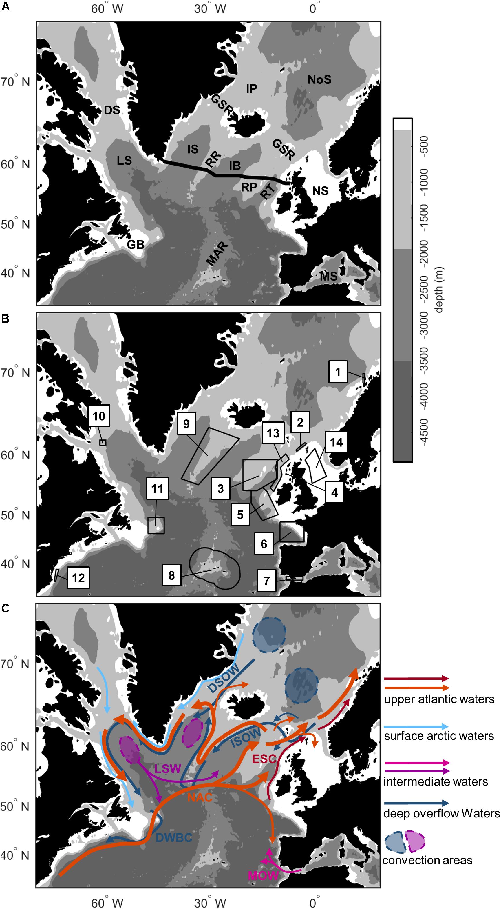
Figure 1. Map of the northern North Atlantic region showing (A) bathymetric features referred to in the text, (B) the 14 case studies chosen to represent a range of Atlantic Vulnerable Marine Ecosystems and management regimes, and (C) a schematic of the circulation. See Table 1 for case study names. Black line in (A) shows the OSNAP-EAST section. Labeled bathymetry: DS, Davis Strait; GB, Grand Banks region; GSR, Greenland-Scotland Ridge; IB, Iceland Basin; IP, Icelandic Plateau; IS, Irminger Sea; LS, Labrador Sea; MAR, Mid-Atlantic Ridge; MS, Mediterranean Sea; NS, North Sea; NoS, Nordic Seas; RR, Reykjanes Ridge; RP, Rockall-Hatton Plateau; RT, Rockall Trough. Contour levels are at 200, 2000, and 3500 m denoting the continental shelves, maximum depth of ARGO floats, and abyssal areas. Labeled currents, DSOW, Denmark Strait Overflow Water; DWBC, Deep Western Boundary Current; ESC, European Slope Current; ISOW, Iceland Scotland Overflow Waters; LSW, Labrador Sea Water; MOW, Mediterranean Overflow Water; NAC, North Atlantic Current.

FIGURE 2

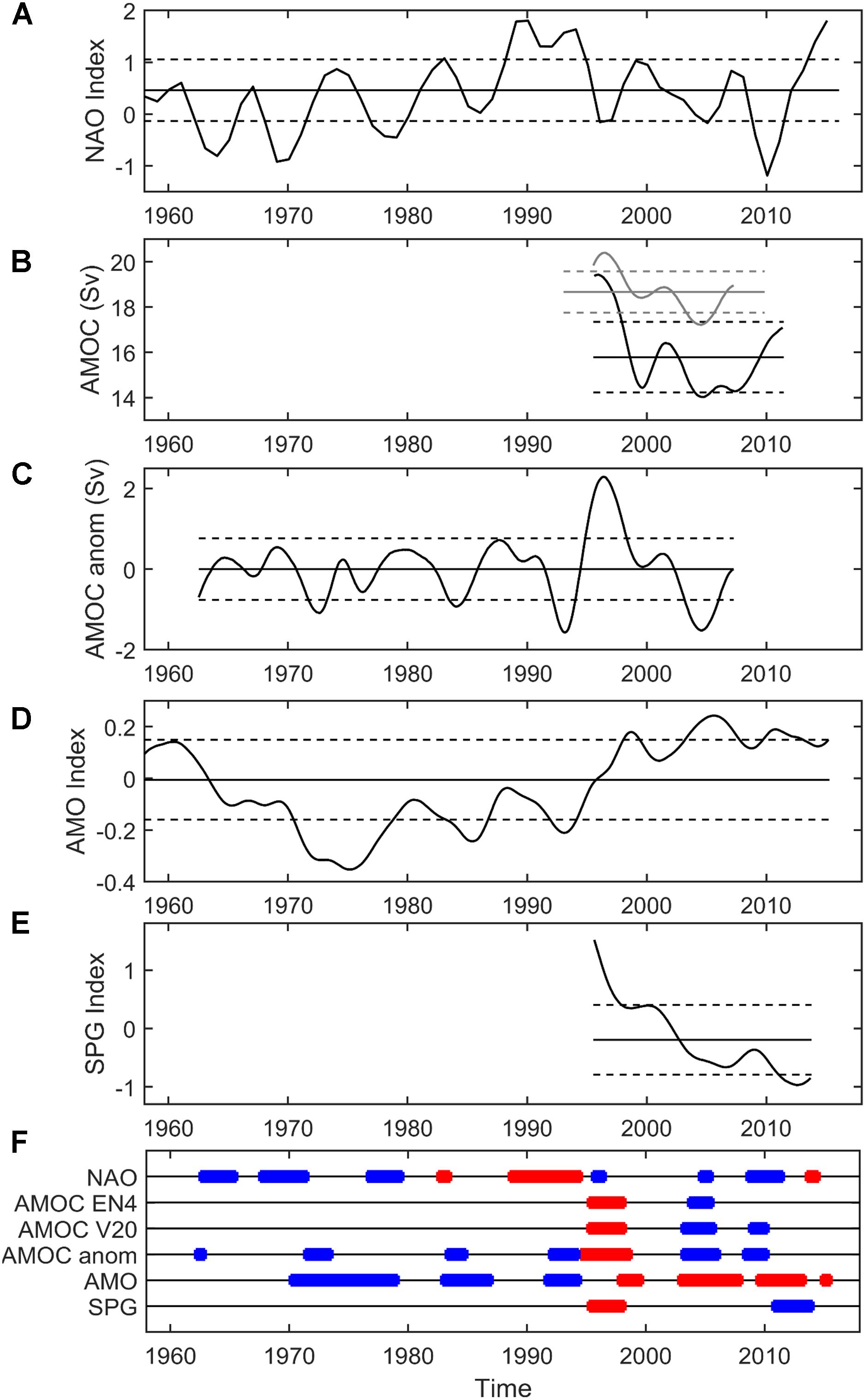
Figure 2. Time-series of climate indices pertinent to the northern North Atlantic region: (A) North Atlantic Oscillation (NAO), (B) Atlantic Meridional Overturning Circulation (AMOC) (black: EN4 time-series, gray: Viking20 time-series post-1993 only), (C) de-trended Atlantic Meridional Overturning Circulation from Viking20, (D) Atlantic Multi-decadal Oscillation (AMO), and (E) Subpolar Gyre (SPG). All time-series have been smoothed using a 5 years Gaussian filter. Solid line shows the mean, and dashed lines ± standard deviation. (F) Shows the high (red) and low (blue) periods for each index that are used in the composite analysis.

North Atlantic Oscillation (NAO)

The NAO is an atmospheric pressure index that influences the position and strength of westerly winds (e.g., Hurrell, 1995) and has several effects on the North Atlantic ocean. Sea surface temperatures show a tripole pattern; during a positive NAO: cooler temperatures are seen south of our study area in the tropical Atlantic, warmer temperatures are observed in the Gulf Stream region in the western Atlantic south of ∼45°N, and cooler temperatures are seen in the main subpolar region centered about Greenland (e.g., Marshall et al., 2001). A further area of warmer temperatures, during a positive NAO, is observed on the western European Shelf extending to the oceanic regions immediately west of the UK and Norway (Visbeck et al., 2013). The NAO also effects the intensity of convection in the Labrador and Nordic Seas, which, along with changes in upper waters, determines the properties of intermediate and deep water masses in those basins (Dickson et al., 1996). A positive NAO is associated with cooler and fresher Labrador Sea Water (e.g., Yashayaev, 2007). This signature is spread through the subpolar gyre along the Labrador Sea Water pathways, although transit times to the eastern basins are in the order of 5–10 years (Yashayaev et al., 2007a, b). In contrast, deep waters in the Greenland Sea are warmer and more saline during a high NAO (Dickson et al., 1996; Alekseev et al., 2001). Finally, Iceland Scotland Overflow Water has a lower salinity during a high NAO (Sarafanov, 2009) with less vigorous flow (Boessenkool et al., 2007). No relationship between Denmark Strait Overflow Water salinities and the NAO is observed (Sarafanov, 2009).

Atlantic Meridional Overturning Circulation (AMOC)

The AMOC is a measure of the strength of the overturning circulation in the important North Atlantic region. This circulation involves the conversion of less dense upper waters to denser intermediate and deep waters, and comprises a northward flow in the upper water column balanced by a return flow at depth. The patterns in upper ocean properties have predominantly been investigated in models, with temperatures showing a dipole signal: during a strong AMOC, cooler temperatures are observed in the Gulf Stream region, and warmer temperatures in the subpolar North Atlantic (Zhang, 2008; Tulloch and Marshall, 2012). In observational datasets, warmer sea surface temperatures in the Gulf Stream region, and cooler sea surface temperatures in the subpolar North Atlantic, have been attributed to a weakening AMOC over the past century (e.g., Caesar et al., 2018). This cooling is most pronounced in the Labrador, Irminger and Iceland Basins.

Atlantic Multi-decadal Oscillation (AMO)

The AMO is a measure of mean sea surface temperature over the entire North Atlantic and exhibits low frequency variability with a periodicity in the order of 65–80 years (Kerr, 2000). A positive index is associated with warmer sea surface temperatures over the region, with the greatest warming observed in the western subpolar gyre (Buckley and Marshall, 2016). During negative phases of the AMO, zonally-averaged sea surface temperature anomalies reveal the cooling is also more pronounced north of around 40° N (Frajka-Williams et al., 2017).

Subpolar Gyre (SPG)

The SPG is a measure of both the strength and extent of the subpolar gyre, with the most commonly used index being the first principal component of the sea surface height field (e.g., Häkkinen and Rhines, 2004; Hátún et al., 2005). During a high SPG, the subpolar gyre is stronger and expands eastward (Thierry et al., 2008). Eastern areas of the subpolar North Atlantic are more strongly influenced by cooler and fresher subpolar water masses, with a reduction in the presence of warmer and saltier subtropical and inter-gyre water masses that enter from the southeast. This change is reflected in upper water properties, with lower temperatures and salinities observed in eastern areas during a high SPG (Holliday, 2003; Johnson et al., 2013). Similarly, at intermediate depths, cooler and fresher conditions are also seen during a high SPG due to the increased influence of Labrador Sea Water and reduced influence of warmer and saltier Mediterranean Water (Lozier and Stewart, 2008).

Data and Methods

In this work, we use an objectively-analyzed observational dataset (EN4) to examine changes in bottom salinity (S_bot) and potential temperature (θ_bot), and output from a high-resolution, eddy-resolving ocean-only model (Viking20) to investigate changes in bottom kinetic energy (KE_bot).

EN4 Data

EN4 is a global, quality-controlled, objectively-analyzed, dataset of observed potential temperature and salinity profiles which has been used extensively (e.g., Prieto et al., 2015; Yang et al., 2016; Zunino et al., 2017; Chafik et al., 2019; Etourneau et al., 2019). It combines data from all types of profiling instruments, including ship-based measurements and ARGO floats, and is available as monthly averages (Good et al., 2013). EN4 has a 1° horizontal resolution meaning that smaller spatial features will not be resolved, and that large property gradients, such as around the boundary of basins, will become smoothed. Although EN4 starts in 1900, we limit our analysis to 1959 onward (to match with Viking20) but extend the analysis until December 2017 to maximize available data.

Bottom potential temperature and salinity were defined as values in the deepest depth bin at any location. The vertical grid in EN4 varies non-linearly with water depth, ranging from 10 m bins in the upper 100 m, to a maximum of ∼300 m below 3000 m. Thus measurements at any location will, at the most, be within 300 m of the sea-bed, with this value reducing as the sea-bed shallows. This vertical resolution is unlikely to greatly impact the representativeness of bottom values when the deep waters are weakly stratified; however, any vertical features smaller than the grid box depth will not be resolved. The EN4 dataset reverts to a 1971–2000 climatology in the absence of any observations (Good et al., 2013). Information for each data point (i.e., for each horizontal grid point, and at each depth level) is given in the weighting variable, which ranges from approximately zero to one. A value of zero indicates the absence of any observations for that data point, during that month, and that climatology is used. Conversely, a weighting of approximately one indicates a high influence of observations. Here we use a cut-off weighting value of 0.1, i.e., we do not use data with a weighting <0.1. This value was chosen to ensure that periods with no observations, where EN4 reverts to a pure climatology, were not included in the analyses, whilst as many observations as possible were incorporated.

Viking20 Data

Viking20 is a 1/20th degree, hindcast-forced, ocean-only model, covering the northern North Atlantic area. It is nested within a global ocean/sea-ice model using the Adaptive Grid Refinement Scheme (Debreu et al., 2008). The model was initiated with climatological temperature and salinity values, and was forced with CORE2 atmospheric data (Large and Yaeger, 2009). More details of the model configuration can be found in Böning et al. (2016). Viking20 has been used in many studies, including those to investigate: the North Atlantic Current (Breckenfelder et al., 2017), convection in the Labrador Sea (Böning et al., 2016), Denmark Strait Overflow Water (Behrens et al., 2017), the Deep Western Boundary Current (Mertens et al., 2014; Handmann et al., 2018), and seasonal changes in the eastern subpolar North Atlantic (Gary et al., 2018).

We use Viking20 output as 5 days averages from 1959 to 2009 to investigate changes in bottom kinetic energy. Bottom horizontal velocities (u_bot, v_bot) were extracted from the bottom grid point at a particular location. As for EN4, grid box thickness varies non-linearly with depth; from <10 m in the upper 50 m, to a maximum of ∼250 m in the deepest points of the model domain. The vertical resolution of Viking20 is not dissimilar to that of EN4, and the same limitations apply. For example, real-world smaller-scale frictional effects, such as benthic boundary layers, will not be resolved in the velocity field. As our goal was to study kinetic energy, rather than velocities, u_bot and v_bot were first linearly interpolated from their respective grids onto the grid containing θ_bot and S_bot. Bottom mean kinetic energy was then calculated as the sum of the squares of mean u_bot and v_bot, with the eddy kinetic energy defined as the sum of the variances of u_bot and v_bot. As our data are 5 days averages, variances represent energy of sub-inertial flows.

Ecosystem Case Studies

As well as considering spatio-temporal patterns at the basin-scale, we examine temporal changes at fourteen case study sites (Figure 1 and Table 1). These sites were chosen to represent a variety of potentially vulnerable deep-sea ecosystems across the northern North Atlantic region as indicated by VME indicator records (Morato et al., 2018). The sites also include a number of existing, or proposed, Marine Protected Areas (MPAs), Ecologically or Biologically Significant Areas (EBSAs), and VME closures (Johnson et al., 2018). Although four sites have maximum depths below 3500 m (Table 1), there is no site that truly represents the abyssal plains of the North Atlantic south of 50°N. This reflects the current absence of VME indicator records in these areas (Morato et al., 2018). Time-series were constructed for each case study site. In EN4, data within each case study polygon were simply averaged for each monthly time-step. As case studies 4 and 10 did not contain any EN4 grid points; time-series for these sites were instead extracted from the nearest EN4 grid point. In Viking20, the model grid is curvilinear. Thus, grid points were accordingly area weighted when calculating averages for each 5 days time-step.

TABLE 1

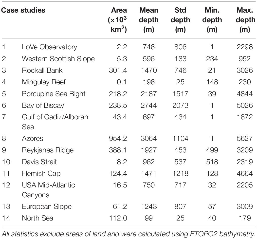
Table 1. Description of case study regions chosen to represent a range of Atlantic Vulnerable Marine Ecosystems and management regimes.

Climate Indices

We consider the four most commonly used climate indices for the North Atlantic Ocean: the NAO, AMOC, AMO, and SPG. The NAO index used is defined as the normalized pressure difference between Gibraltar and southwest Iceland (Jones et al., 1997). Data were downloaded from the Climatic Research Unit¹ and the winter (DJFM) mean calculated. As Viking20 is forced with CORE2 atmospheric data, which will include a signature of the NAO, we use the observational NAO time-series to investigate ocean correlations in both the EN4 and Viking20 datasets.

For the AMOC, we use the commonly used definition of the maximum in the overturning stream function in density space (e.g., Mercier et al., 2015; Lozier et al., 2019). As this index is calculated from oceanic rather than atmospheric variables, and changes in the model and observational AMOC may not be contemporaneous, we compute two AMOC time-series: one from EN4 and one from Viking20. For the observational dataset we used the method of Mercier et al. (2015), but using EN4 data along the OSNAP-EAST section (black line, Figure 1A). Geostrophic velocities perpendicular to the section were calculated from EN4 temperature and salinity data and referenced to satellite altimetry data. The Viking20 AMOC time-series was calculated using model velocities perpendicular to the OSNAP-EAST section.

We use an AMO index downloaded from the National Oceanic and Atmospheric Administration² as monthly averages. This time-series consists of sea surface temperatures, averaged over 0–70°N before de-trending using a 10 year running mean (Enfield et al., 2001). The AMO is also an oceanic index, suggesting that again a model and observational time-series is required. Although the construction of an AMO index from Viking20 was considered, it was discounted for two reasons. Firstly, the AMO index is calculated using sea surface temperatures over the entire North Atlantic; however, the Viking20 nested model domain starts at 32° N (Böning et al., 2016). This makes the calculation of an AMO index from Viking20 more complex. Secondly, Viking20 is an ocean-only model meaning that feedbacks between the ocean and atmosphere are not fully represented. As previous work suggests there is a requirement for fully-coupled models in order to represent important teleconnections (Ruprich-Robert et al., 2017), we focus on the observational AMO index and therefore do not investigate changes in KE_bot using Viking20.

The SPG index used is defined as the first principal component of the sea surface height field between 40 and 65° N and 60° W to 10° E (Berx and Payne, 2017). This was downloaded from https://data.marine.gov.scot/dataset/sub-polar-gyre-index as monthly averages. Again, we considered extracting out a model-based SPG time-series from Viking20 to use in conjunction with the observational index. However, the basin-averaged sea surface height field in Viking20 exhibits a drift after the mid-1990s, which would redistribute power among the principal components used to generate the SPG index. As such, we again focus on the observational SPG and interrogate only the EN4 dataset. Although there may be a large-scale drift in the Viking20 sea surface height field, gradients in sea surface height and the overall circulation patterns in the model output compare well to observations (e.g., Breckenfelder et al., 2017; Gary et al., 2018).

Composite Method

In order to investigate any differences in near-bed conditions associated with each climate index, we use the commonly-used composite method (e.g., Terray et al., 2003; Häkkinen et al., 2011; Tulloch and Marshall, 2012). For each climate index, “high years” were defined as those exceeding one standard deviation above the mean, and “low years” as those less than one standard deviation below the mean. Composites for the high and low climate states were calculated by averaging properties from all high and low years respectively. One of the limitations of the composite approach is that it only considers high and low states, and not transitional processes between the two. As the Viking20 AMOC time-series shows a long-term trend and we are interested in multi-annual changes, we de-trended this index before creating the composites. The time-series was de-trended by assuming a linear long-term trend which may not be entirely appropriate for low-frequency oscillations. However, the record is too short to establish any low-frequency variability more accurately, and de-trending enables us to investigate multi-annual changes over a 50 year period. The number of months averaged to create each composite are shown in Table 2.

TABLE 2

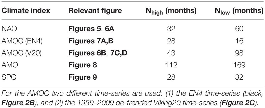
Table 2. Number of months used to create the high and low composites for each climate index: North Atlantic Oscillation (NAO), Atlantic Meridional Overturning Circulation (AMOC), Atlantic Multi-decadal Oscillation (AMO), and Subpolar Gyre (SPG).

The statistical significance of observed changes at the 95% confidence level were tested using the method detailed in Terray et al. (2003), which we briefly describe here. At each grid point (X), we assess whether the values observed during the high years, or the low years (class j), are significantly different from a combined group made up of high and low years only. The years within one standard deviation from the mean are not included because the composite analysis only compares two groups: high and low years. The mean of class j ($\overline{x_j})$is therefore compared to the mean of the combined high and low time-series ($\overline{x}$), with respect to the standard error (Equations 1, 2).

$$U\left(X\right)=abs((\overline{x_j}-\overline{x})/s_j)(1)$$

$$s_j=\sqrt{(n-n_j)/(n_j\times \left(n-1\right))}\times s(2)$$

where: s is the standard deviation of the combined high and low time-series; and n and n_j the number of data points in the combined time-series and class j respectively.

This procedure tests whether or not the high and low years were allocated randomly from the combined group. If the high years and low years are allocated randomly, U(X) will approach zero. Hence, the larger U(X), the more diverse the high and low years, and the less likely that the high and low years were randomly selected. It should be noted that U(X) calculated with the high years as class j, is identical to U(X) calculated with the low years as class j. We set the critical value as 1.96, with values of U(X) exceeding this indicating that the two means are statistically significantly different at the 95% confidence level.

Results: Long-Term Mean State

In order to provide a baseline for interpreting temporal changes, we first present the long-term mean and associated variability as basin-wide maps. Since the variability of shallower waters can be orders of magnitude larger than that of deeper waters, the variability maps are shown on a log₁₀ scale to highlight the changes over the whole domain. We use the objectively-analyzed observational dataset (EN4) to investigate changes in S_bot and θ_bot (Figure 3), and output from a high-resolution model (Viking20) to examine changes in KE_bot (Figure 4).

FIGURE 3

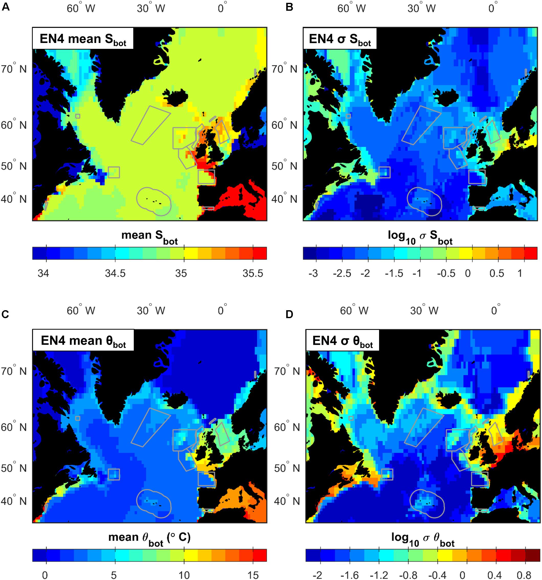
Figure 3. Maps of mean (A) bottom salinity and (C) potential temperature (°C) between 1959–2017 in EN4, and associated standard deviations (B,D). Gray boxes show case study areas. To fully resolve variability across bathymetric-depths, (B,D) are shown on a log₁₀ scale.

FIGURE 4

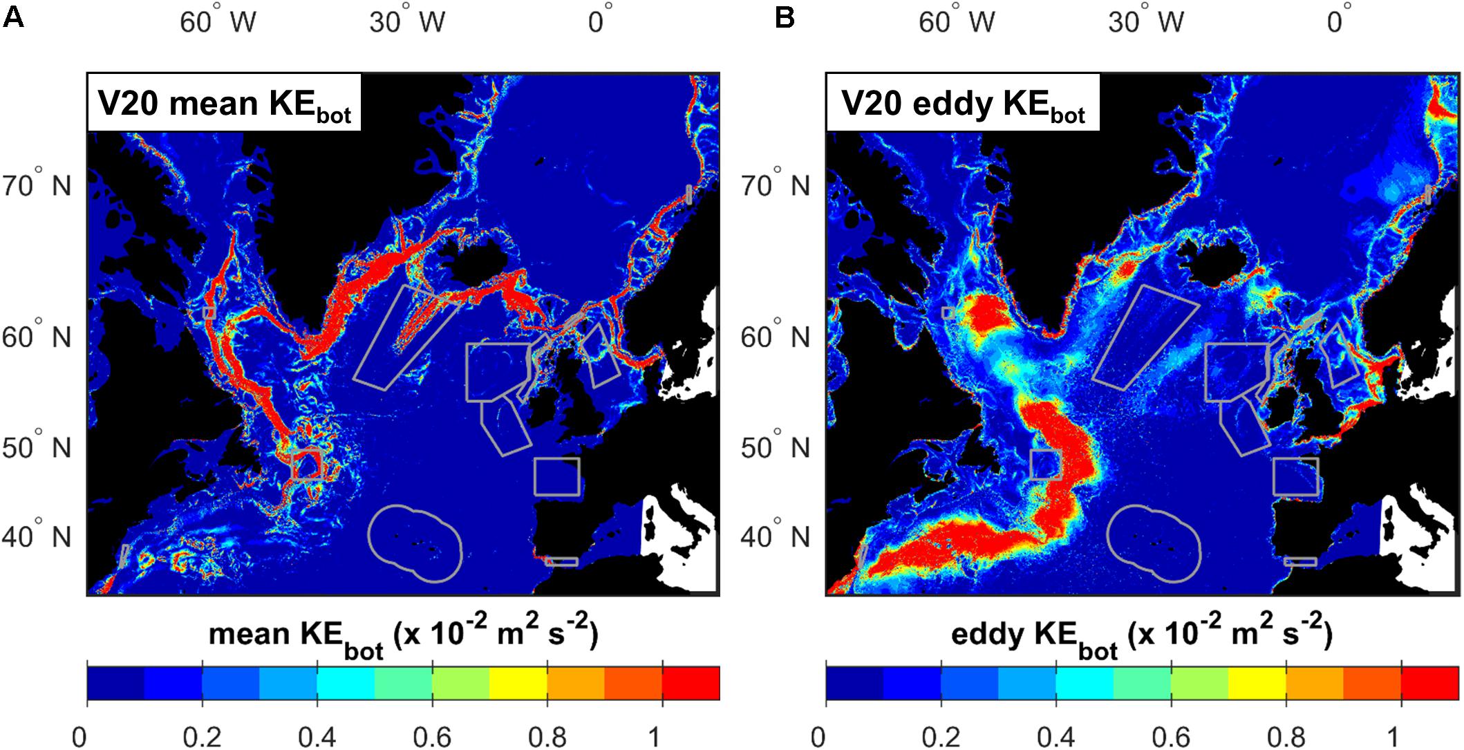
Figure 4. Maps of (A) mean bottom kinetic energy and (B) associated eddy kinetic energy (×10^–2 m²s^–2) from 1959 to 2009 in Viking20. Gray boxes show case study areas.

The lowest mean S_bot values are seen on the North American Shelf (<34.0) and in the Baltic Sea (<10.0), whilst the highest S_bot values are seen in the Mediterranean Sea (>37.0) and on the European Shelf west of the UK and Ireland (35.40–35.55) (Figure 3A). Relatively high S_bot values are also seen over the shallower Rockall-Hatton Plateau (35.0–35.3), over the eastern Greenland-Scotland Ridge (35.0–35.2), and along the Norwegian Coast (35.0–35.2). In contrast, fresher conditions (34.4–34.7) are seen north of the Davis Strait. Bottom salinity in areas deeper than ∼2000 m is fairly uniform (34.85–35.00), although S_bot decreases with water depth, and slightly more saline bottom conditions are observed in eastern parts of the subpolar region. There is little difference between S_bot values in the northern North Atlantic and Nordic Seas.

Variability in S_bot is strongly related to water depth (Figure 3B), with the highest variability on the continental shelves (±0.1–0.4), and the lowest variability seen in areas deeper than 2000 m (±<0.01). However, there is also spatial variability within these general descriptions. For example, variability is higher in the southern North Sea compared to the northern North Sea and shelf areas west of the UK and Ireland.

The highest θ_bot values (>15°C) are seen on the North American Shelf south of around 40°N and in the Mediterranean Sea (>12°C) (Figure 3C). Relatively high values are also seen in the southern North Sea and on the European Shelf west of the UK and Ireland (10–12°C). The coldest bottom conditions (<0°C) are seen in the Nordic Seas and north of the Davis Strait. In contrast, θ_bot values in the northern North Atlantic range from 1 to 3°C with an east-west split. Warmer θ_bot values are seen in areas shallower than approximately 2000 m, such as over the Greenland-Scotland Ridge (3–5°C), around the boundaries of the subpolar basins (3–5°C), and over the Rockall-Hatton Plateau (4–7°C).

Variability in θ_bot is again mainly constrained by water depth (Figure 3D), with the highest values observed in the southern North Sea (±2.0–4.0°C) and on the North American Shelf (±1.5–3.0°C). In contrast, lower variability is observed in the deep northern North Atlantic and Nordic Seas (±<0.04°C). In the subpolar North Atlantic, higher variability (0.04–0.06°C) is observed in the Labrador Sea and Irminger Sea compared to the more eastern basins.

The highest KE_bot (>10 × 10² m²s^–2) (Figure 4A) is associated with the flow of Denmark Strait Overflow Water in the Irminger Sea, and Iceland Scotland Overflow Water in the Iceland Basin. In addition, high KE_bot values (1–10 × 10^–2 m²s^–2) are observed in the cyclonic boundary currents of the subpolar gyre, including around the boundary of the Labrador Sea and in the Deep Western Boundary Current. Energetic conditions (>1 × 10^–2 m²s^–2) are also associated with the European Slope Current along the northern European and Norwegian Shelves. Other areas, such as the deep northern North Atlantic and Nordic Seas, have low KE_bot (<0.1 × 10^–2 m²s^–2).

The highest values of eddy KE_bot (1–2 × 10^–2 m²s^–2) (Figure 4B) are associated with the Deep Western Boundary Current, although this is over a wider spatial area than the higher KE_bot signal. High eddy KE_bot values (∼1 × 10^–2 m²s^–2) are likewise associated with the overflow currents, as well as in the convection areas of the Labrador and Irminger Seas. High eddy KE_bot is also seen in the European Slope Current, although this is of lower magnitude than that seen for the deeper currents. Finally, areas of higher eddy KE_bot are seen on the continental shelves; including in the southern North Sea, on the North American Shelf south of around 40°N, and on both the East and West Greenland Shelves.

Results: Spatial Variability Linked to Climate Indices

Having described the long-term mean and variability, we now examine changes associated with each climate index in turn using the composite approach detailed in section Composite Method. Again, we use the objectively-analyzed observational EN4 dataset to investigate changes in S_bot and θ_bot, and output from the Viking20 model to examine changes in KE_bot. For EN4, we only describe changes where a cut-off weighting is exceeded for both the high and low composites; this ensures the exclusion of periods with no observations. Plots comparing the spatial footprint of different cut-off weightings, ranging from 0.05 to 0.25, are shown in Supplementary Figures S1–S4. For the NAO, the spatial distribution of data for cut-off values ranging from 0.1 to 0.25 is almost identical. For the AMOC, AMO, and SPG there are some small differences; for example: in the eastern Nordic Seas and around the Reykjanes Ridge for the AMOC, in the eastern Nordic Seas and Iceland Basin for the AMO, and in the eastern Nordic Seas for the SPG. However, all cut-off weightings retain data: on the continental shelves, around the boundaries of the basins of the subpolar North Atlantic, over the Reykjanes Ridge, over the Greenland-Scotland Ridge, over the Icelandic Plateau, and around the boundaries of the Nordic Seas. We chose a cut-off weighting of 0.1 to retain as many observations as possible, with only areas where this is exceeded for both the high and low composites included. Although there is a level of subjectivity when choosing the EN4 cut-off weighting, as an additional control we carried out statistical testing (as detailed in section Composite Method). Only changes between the high and low years that are statistically significant at the 95% confidence level are discussed. As pure climatology would have no significant correlations, we can be sure that any statistically significant patterns are due to the presence of data.

North Atlantic Oscillation (NAO)

The largest changes in S_bot and θ_bot associated with the NAO are observed on the continental shelf areas (Figure 5). The European and North American Shelves are anti-correlated: when the NAO is high, warmer and more saline bottom conditions are seen in the North Sea but cooler and fresher values are seen around Grand Banks. Whilst bottom conditions in the Grand Banks area are −0.5 to −1.3°C cooler, and −0.1 to −0.25 fresher, during a high NAO period relative to a low NAO period, the North Sea bottom values are 1.0–1.3°C warmer and 0.2–1.2 saltier. The area to the west of Norway is also 0.03–0.5°C warmer during high NAO periods compared to low NAO periods, although a corresponding S_bot signal is absent.

FIGURE 5

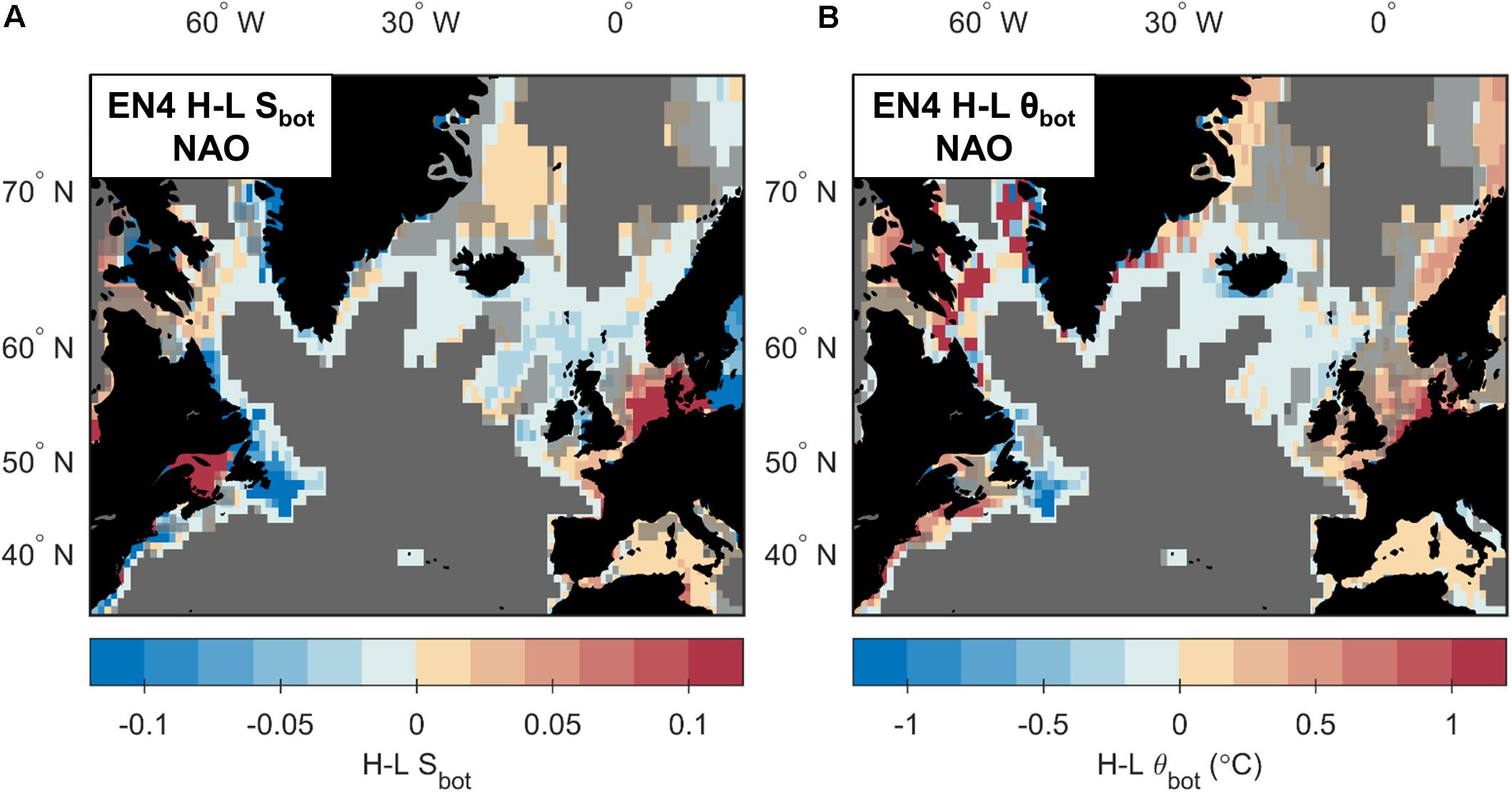
Figure 5. Maps of differences in bottom conditions between high and low states of the North Atlantic Oscillation (NAO) in EN4: (A) bottom salinity changes and (B) bottom potential temperature changes. Transparent gray shading shows areas where the H minus L is not statistically different at the 95% confidence limit, and solid gray shading areas with an EN4 weighting of <0.1 for either the high or low years.

When investigating signals away from the continental shelves, there is limited observational data, particularly below 2000 m. Nevertheless, some spatially coherent and statistically significant changes can be seen. In the Mediterranean Sea, warmer and saltier bottom conditions (0–0.3°C and 0–0.02) are observed during a high NAO. In contrast, lower S_bot and θ_bot values (<−0.02 and <−0.2°C respectively) are seen in the subpolar gyre, for example around the boundaries of the Labrador Sea and Irminger Sea, over the Reykjanes Ridge, and over the Rockall-Hatton Plateau. In particular, less saline bottom conditions (−0.02 to −0.04) are observed in eastern areas extending on to the shelf west of Scotland, and over the Greenland-Scotland Ridge along pathways of the North Atlantic Current and European Shelf Current.

Viking20 output can be used to evaluate changes in KE_bot (Figure 6A). During a high NAO, bottom currents are enhanced along the eastern boundary of the northern North Atlantic with higher KE_bot stretching along the European and Norwegian Shelf break, and into the North Sea. This is likely to indicate a stronger European Slope Current during a high NAO. Higher KE_bot is also observed along the Denmark Strait Overflow Water pathways around the western boundary of the Irminger Sea, although lower KE_bot values are seen around the northern and western boundaries of the Iceland Basin which is influenced by Iceland Scotland Overflow Water. Finally, lower KE_bot is seen on shelf areas to the north and west of the Labrador Sea.

FIGURE 6

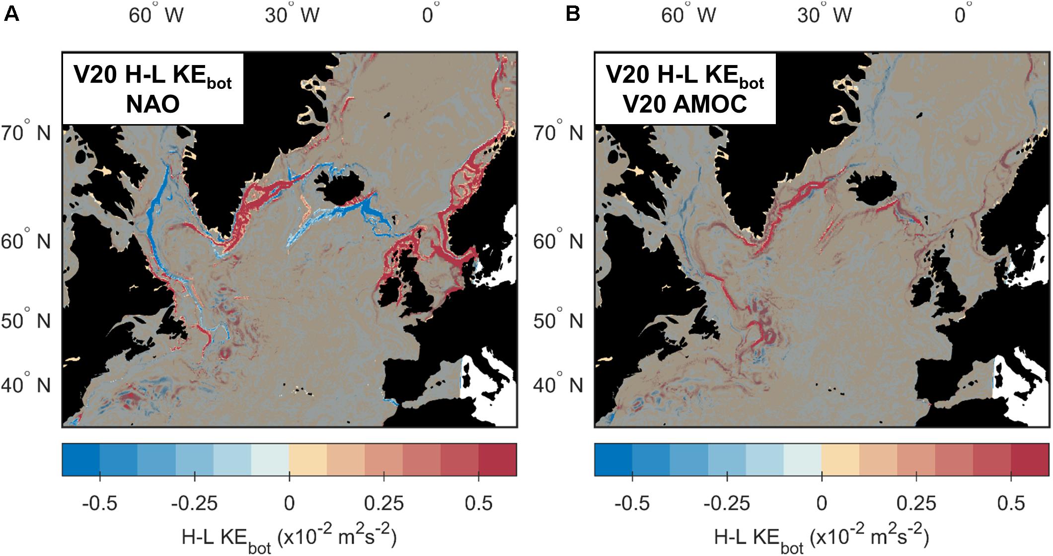
Figure 6. Maps of differences in bottom kinetic energy in Viking20 between the high and low states of the (A) North Atlantic Oscillation (NAO) and (B) de-trended 1959–2009 Atlantic Meridional Overturning Circulation (AMOC). Transparent gray shading shows areas where the H minus L is not statistically different at the 95% confidence limit.

Atlantic Meridional Overturning Circulation (AMOC)

To investigate changes associated with the AMOC, we start by using the post-1993 observational AMOC time-series to examine changes in the EN4 dataset (Figures 7A,B). The North American, European and Norwegian Shelves all have lower S_bot values (−0.1 to −0.5) during high AMOC states. While θ_bot values are also lower (−0.4 to −0.8°C) on northern parts of the North American Shelf and around Grand Banks during a high AMOC, south of around 50°N warmer (0.5–2.5°C) bottom conditions are seen. Additionally, on the European Shelf, statistically significant changes in θ_bot (−0.4 to −0.8°C) are only observed in the northern areas of the North Sea. The lower θ_bot values during a high AMOC on the Norwegian Shelf are also less pronounced than the observed freshening. Hence, on the continental shelves, changes in S_bot and θ_bot associated with the NAO are not simply correlated.

FIGURE 7

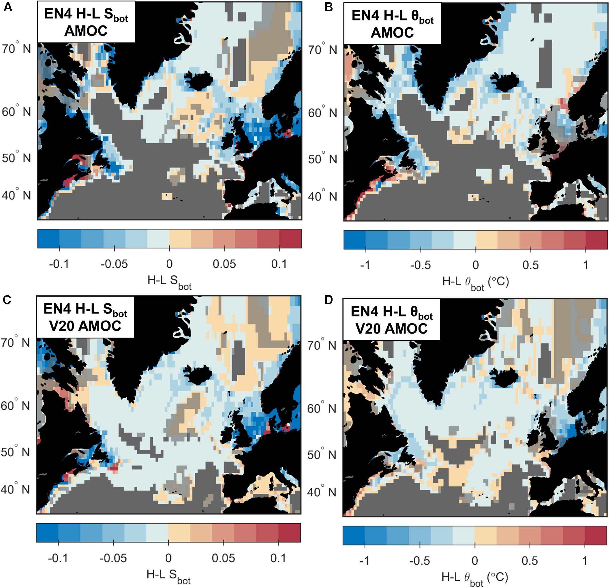
Figure 7. Maps of differences in bottom conditions between high and low states of the Atlantic Meridional Overturning Circulation (AMOC) in EN4: (A) bottom salinity changes and (B) bottom potential temperature changes constructed using the EN4 AMOC time-series, and (C) bottom salinity changes, and (D) bottom potential temperature changes constructed using the de-trended 1959–2009 Viking20 AMOC time-series. Transparent gray shading shows areas where the H minus L is not statistically different at the 95% confidence limit, and solid gray shading areas with an EN4 weighting of <0.1 for either the high or low years.

Moving now to oceanic areas, fresher and in particular cooler conditions are seen in most regions during a high AMOC. The largest changes (up to −0.35°C and −0.05) are seen around the boundaries of the Labrador Sea, Irminger Sea and Iceland Basin, as well as over the Greenland-Scotland Ridge. Although S_bot and θ_bot are lower during a high AMOC in the majority of areas, warmer and more saline bottom conditions are also seen. For example, the Rockall Trough and eastern Iceland Basin are up to 0.011 more saline during a high AMOC. More saline conditions are also observed in the eastern Nordic Seas. In contrast, areas of warmer bottom conditions during a high AMOC are patchy. Despite the higher S_bot values in the Rockall Trough during a high AMOC, fresher (0 to −0.05) conditions are still observed over the shallower Rockall-Hatton Plateau and on the European Shelf west of the UK.

As the timing of changes in strength between the observational and modeled AMOC compare extremely well during the contemporaneous period (Figures 2B,F), we now use the de-trended Viking20 AMOC time-series to interrogate the EN4 dataset (Figures 7C,D). Applying the Viking20 AMOC time-series to the EN4 data assumes that the relationship between the observed and modeled AMOC persists outside the post-1993 era. However, the advantage is that it increases the amount of observational data used in the construction of the composites (Table 2) therefore increasing the spatial extent of the analysis.

Many spatial features observed in the composites created using the observed AMOC time-series (Figures 7A,B), are also seen in those created from the de-trended Viking20 AMOC time-series (Figures 7C,D). However, the magnitude of changes are often lower in the model AMOC composites. The extended selection period for the ocean observations is particularly noticeable in the relatively data-sparse areas deeper than 2000 m. Changes in bottom conditions are now revealed in the central Labrador and Irminger Seas, and for areas between approximately 40–52°N, which in the observational AMOC composite had a mean EN4 weighting of <0.1 and were therefore grayed out. Bottom conditions in the central Labrador Sea and Irminger Sea are also cooler (<−0.02) and fresher (<−0.2°C) during a high AMOC. While fresher conditions are seen south of approximately 52°N, warmer θ_bot values are seen in western areas.

Finally, we use Viking20 and the modeled AMOC time-series to examine changes in KE_bot. We present a high minus low map created from the longer de-trended time-series (Figure 6B), which is very similar to the composite compiled from the post-1993 time-series in Viking20 (not shown). Stronger bottom currents are seen around the northern and western boundaries of the subpolar gyre as well as around Grand Banks. KE_bot in these areas is 0.5–1.5 × 10^–2 m²s^–2 greater during a high AMOC than a low state. Although changes are seen along the European and Norwegian Slopes, these are not statistically significant.

Atlantic Multi-decadal Oscillation (AMO)

As discussed in section Climate Indices, it is not appropriate to apply the AMO time-series to output from Viking20; thus we examine changes using the EN4 dataset only and do not discuss KE_bot. High minus low values for the AMO are positive on the North American, Western European, and Greenland Shelves (Figure 8), with bottom conditions 0.6–1.0°C warmer and 0.02–0.2 more saline during a high AMO. Warmer and saltier conditions are also seen over the shallower Greenland-Scotland Ridge where S_bot and θ_bot are up to 0.8°C warmer during a high AMO state relative to a low AMO state, and up to 0.06 more saline. In regions deeper than 2000 m, there is a split between areas north and south of the Greenland-Scotland Ridge. In the deep Nordic Seas, θ_bot and S_bot are higher during a high AMO. In contrast, cooler and less saline bottom conditions are seen below approximately 2000 m in the northern North Atlantic. The magnitude of the changes in θ_bot and S_bot in both these regions are ± 0–0.02 and ± 0–0.2°C respectively. There is insufficient data to assess any changes in areas deeper than 2000 m south of around 45–50°N.

FIGURE 8

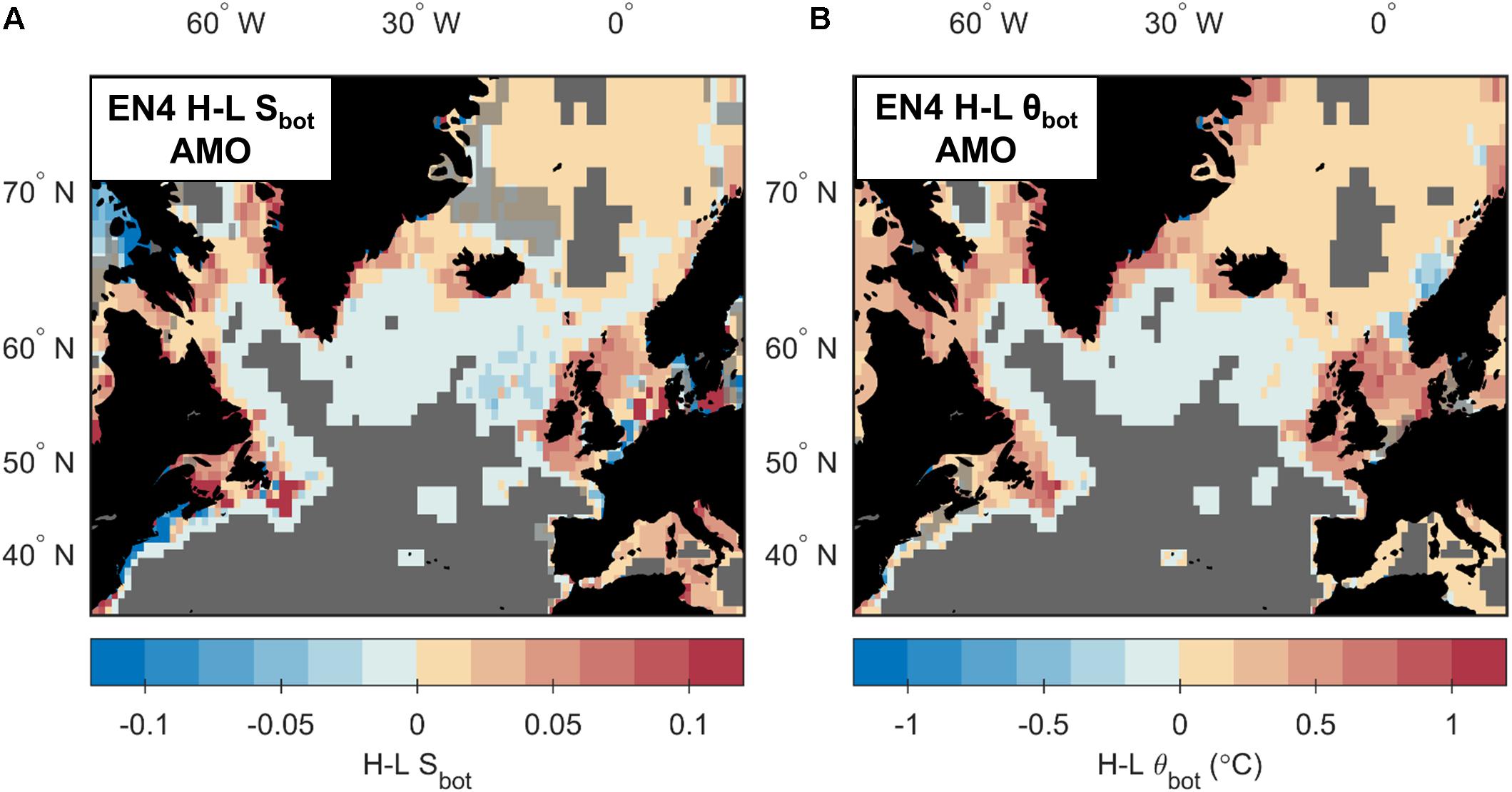
Figure 8. Maps of differences in bottom conditions between high and low states of the Atlantic Multi-decadal Oscillation (AMO) in EN4: (A) bottom salinity changes and (B) bottom potential temperature changes. Transparent gray shading shows areas where the H minus L is not statistically different at the 95% confidence limit, and solid gray shading areas with an EN4 weighting of <0.1 for either the high or low years.

Subpolar Gyre (SPG)

For the SPG, we again only examine changes in the EN4 dataset. Bottom conditions are cooler and fresher during a high SPG for the vast majority of the northern North Atlantic region regardless of bathymetric depth (Figure 9). On the continental shelves, lower S_bot values are seen on the North American (−0.15 to −0.50), European (−0.04 to −0.25) and Norwegian Shelves (−0.04 to −0.08). However, decreased θ_bot values are observed only on the North American shelf (−0.8 to −1.5°C) with the absence of a cooling in the North Sea. On the Norwegian Shelf, cooler bottom waters are only seen north of approximately 70°N, even though the change in S_bot is widespread. Hence, whilst S_bot and θ_bot co-vary on the North American Shelf, this relationship does not exist in the North Sea and Norwegian Shelf. Despite the lack of a statistically robust temperature signal in the North Sea, lower θ_bot values (−0.2 to −0.8°C) are still observed on the European Shelf west of Scotland during a high SPG.

FIGURE 9

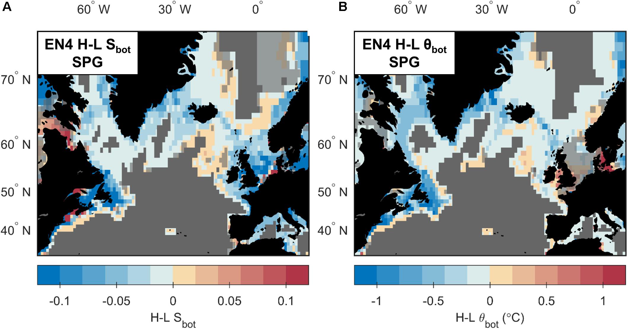
Figure 9. Maps of differences in bottom conditions between high and low states of the Subpolar Gyre (SPG) in EN4: (A) bottom salinity changes and (B) bottom potential temperature changes. Transparent gray shading shows areas where the H minus L is not statistically different at the 95% confidence limit, and solid gray shading areas with an EN4 weighting of <0.1 for either the high or low years.

Away from the continental shelves, fresher and cooler conditions are observed in the majority of areas during a high SPG. Changes are particularly pronounced around the boundaries of the Labrador and Irminger Seas, and over the Reykjanes and Greenland-Scotland Ridges. In these areas, bottom conditions are −0.02 to −0.06 fresher during a high SPG, relative to a low SPG, and −0.2 to −0.8°C colder. Cooler (0 to −0.1°C) and fresher (0 to −0.01) conditions are also observed in areas of the Labrador and Irminger Seas deeper than 2000 m, although these changes are smaller than those observed at the boundaries. In the eastern subpolar gyre, there are some areas of higher θ_bot and S_bot. In particular, bottom conditions in the Iceland Basin and Rockall Trough are up to 0.015 more saline during a high SPG than a low SPG. North of the Greenland-Scotland Ridge, the majority of the Nordic Seas show lower θ_bot values during a high SPG. However, again there are areas of more saline S_bot values, mainly in the eastern portions of the region.

Finally, we note that the pattern of changes in S_bot and θ_bot seen between the high and low states of the SPG (Figure 9), are very similar to that seen for the AMOC; particularly when considering the post-1993 AMOC time-series (Figures 7A,B). Although this may reflect a link between the two climate indices, the selection periods for the two indices are very similar (Figure 2F): the months used to create the high SPG average are almost identical to those used to create the post-1993 high AMOC composite, whilst the input periods for the low composites are sequential to each other. This suggests that a similar signal may be represented for both indices, and thus it is hard to define whether the observed changes are dominated by the SPG, or the AMOC, or indeed whether the two indices act in unison.

Comparison Between Indices

We now examine the spatial dominance of each index by asking a simple question: which climate index is associated with the largest changes at each location? This enables us to examine whether there are spatially coherent patterns, and how these vary both in the horizontal and vertical. As we have investigated more climate indices in EN4, we focus on the changes in S_bot and θ_bot. Again, we only consider changes that are statistically significant at the 95% confidence level, and where there is a weighting >0.1 for both the high and low composites. Although the patterns of variability for the AMOC and SPG are very similar, we include both indices separately to see if perhaps there is a spatial difference between the two.

The dominant climate index pattern is reasonably similar for S_bot and θ_bot, although they are not identical (Figure 10). Whilst some areas are patchy, there are also some spatially coherent signals and general observations to be made. For example, where there is sufficient data to assess changes below 2000 m, the AMO is associated with the largest changes. This is true both in the Nordic Seas and northern North Atlantic. In contrast, the SPG dominates changes in areas shallower than 2000 m in the western subpolar North Atlantic, whilst the AMOC becomes more important in eastern areas. In the Mediterranean Sea, the NAO is associated with the largest changes, particularly when considering θ_bot. Changes on the North American Shelf are dominated by the SPG, whereas the shelf west of the UK is dominated by the AMO. In the North Sea the AMO also dominates changes in θ_bot, whilst the AMOC is more important for changes in S_bot.

FIGURE 10

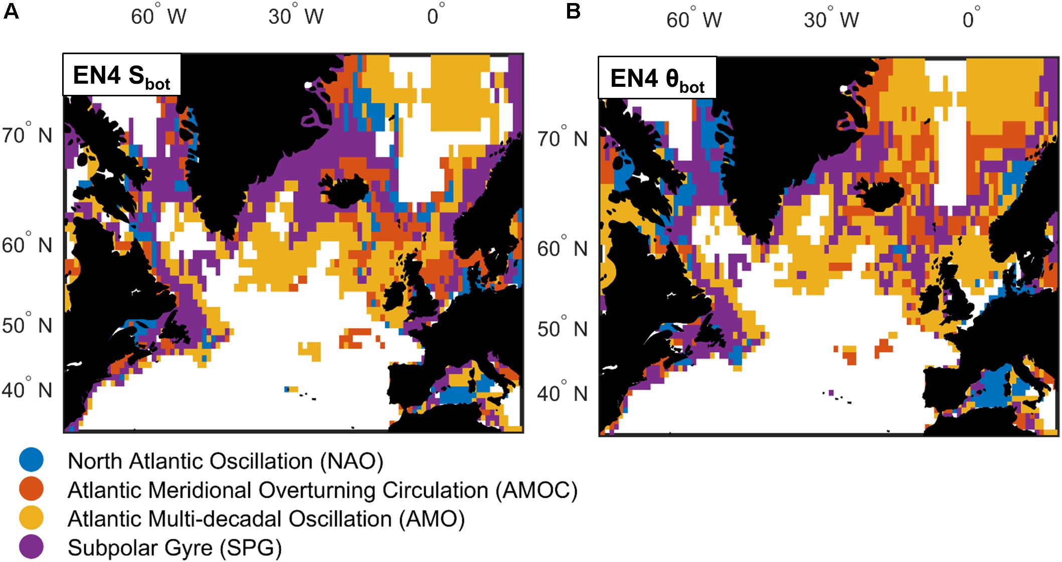
Figure 10. Map summarizing the climate index associated with the largest change in: (A) bottom salinity, and (B) bottom potential temperature, in EN4. Colors correspond to the dominant climate index, with white areas showing areas where no climate index has significant differences at the 95% confidence level, and EN4 weightings >0.1 for both the high or low years.

Results: Variability at Ecosystem Case Study Sites

We now move on to discussing changes at fourteen case studies (Figure 1 and Table 1) chosen to represent various VMEs across the northern North Atlantic region. As these sites cover a number of management measures, such as ESBAs, MPAs, and VME closures, and are therefore often considered as a single entity, we show mean conditions averaged across each location. However, we caution that most case studies cover a range of depths (Table 1), which may be subject to different processes and signals, as well as lag periods. As such, changes at a particular depth may be different to the mean conditions for the entire case study site. For example, at Case Study 9 on the Reykjanes Ridge (Figure 1), the SPG is associated with the largest changes in S_bot in areas shallower than approximately 2000 m, whilst the largest changes in deeper areas are linked to the AMO (Figure 10). Additionally, if signals at different depths are opposing, changes averaged across the case study as a whole may be muted, despite statistically significant changes in individual depth layers. Similar effects will be produced in spatially heterogeneous areas, for example at case study 14 in the northern North Sea (Figure 1). Here, the AMOC is associated with the largest changes in S_bot in southern areas, whilst the largest changes in the northern part of the case study region is associated with the AMO (Figure 10). However, when the S_bot changes are averaged over the entire case study region, only the AMO is associated with statistically significant changes. Finally, as changes are often larger at shallower depths, case study averages are likely to be biased toward processes occurring higher in the water column. As such, we advise the reader to consider the results in this section in conjunction with Section Results: Spatial Variability Linked to Climate Indices and Figures 5–10.

We again use the EN4 dataset to examine changes in S_bot and θ_bot, and output from Viking20 to investigate changes in KE_bot although this is only for the NAO and AMOC. Time-series for each case study site are shown in Supplementary Figures S5–S18, whilst changes between high and low climate states are summarized in Figure 11 and Tables 3, 4. Again we consider the AMOC and SPG separately, and only describe changes in EN4 where the mean data weighting over the case study as a whole exceeds 0.1 for both the high and low states.

FIGURE 11

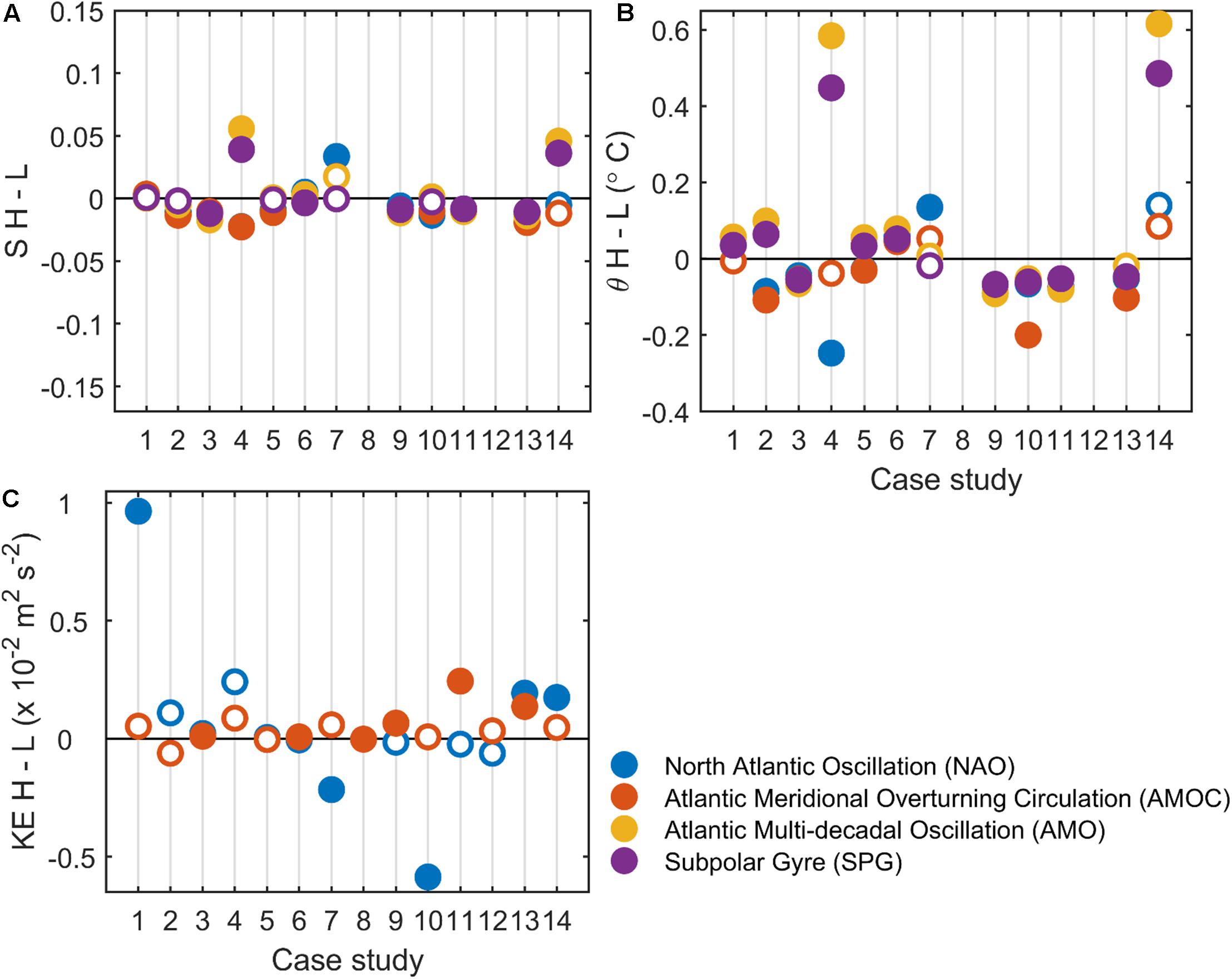
Figure 11. Summary of changes associated with each climate index at the fourteen case study sites: (A) EN4 bottom salinity changes, (B) EN4 bottom potential temperature changes, and (C) Viking20 bottom kinetic energy changes. Filled circles represent changes significant at the 95% level, whilst unfilled circles show non-significant changes. Changes in EN4 where the data weighting is <0.1 for either the high or low composite are not shown. The AMOC in (A,B) represents the EN4 time-series, whilst the AMOC in (C) represents the post-1993 time-series from Viking20.

TABLE 3

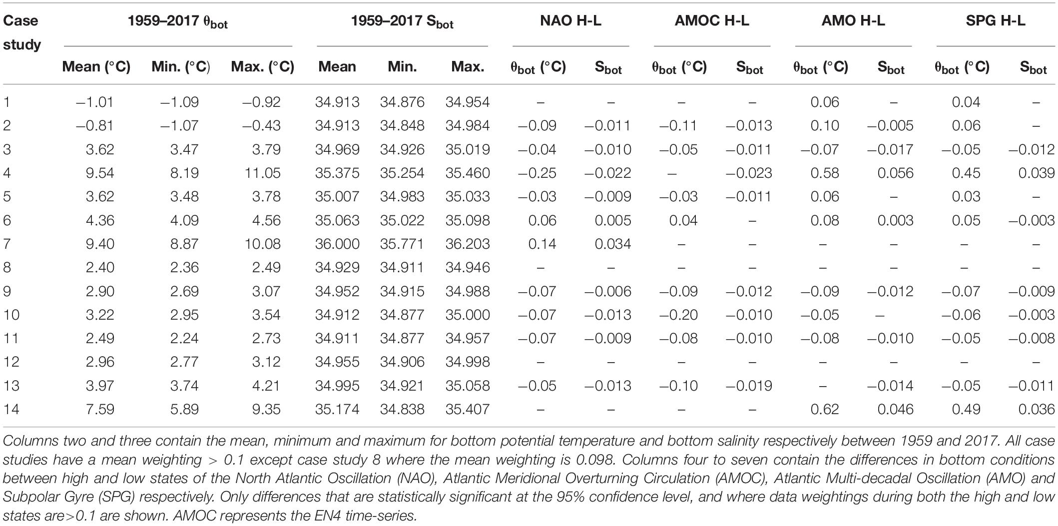
Table 3. Summary statistics from EN4 for the 14 case studies detailed in Table 1.

TABLE 4

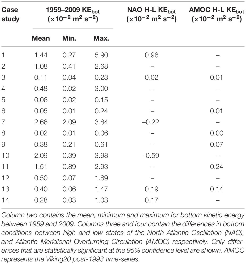
Table 4. Summary statistics from Viking20 for the 14 case studies detailed in Table 1.

Case study 1 is situated on the Norwegian Coast. Here, only changes in θ_bot associated with the AMO and SPG are statistically significant at the 95% confidence level. Both indices show warmer θ_bot during high states, with the AMO having the largest change at 0.06°C. A large positive change in KE_bot (0.96 × 10^–2 m² s^–2) is also observed between high and low states of the NAO. At case study 2, on the western Scottish Slope, all climate indices are associated with significant changes in θ_bot. The NAO and AMOC have cooler θ_bot values during the high states, whilst the AMO and SPG show warmer θ_bot values. The NAO, AMOC, and AMO all produce similar magnitude changes. With respect to S_bot, only the NAO, AMOC, and AMO show statistically significant changes, with all having fresher S_bot values during a high state. The largest changes are associated with the AMOC (−0.013) and NAO (−0.011), with the change between high and low states of the AMO half of these values. No statistically significant changes in KE_bot are seen.

Case study 3 is at Rockall Bank. Here, changes in both θ_bot and S_bot are statistically significant for all climate indices. Cooler and fresher θ_bot and S_bot values are observed during high states. The largest change is associated with the AMO for both θ_bot (−0.07°C), and S_bot (−0.017). Changes in KE_bot though statistically significant are small (0.01–0.02 × 10^–2 m²s^–2). Case study 4, which has an average depth of 196 m and covers the Mingulay Reef complex to the west of Scotland (Roberts et al., 2009), shows large changes. Statistically significant changes in θ_bot are seen for the NAO, AMO, and SPG. The NAO has cooler θ_bot during a high state, whilst the AMO and SPG exhibit warmer θ_bot. All climate indices show significant changes in S_bot. The NAO and AMOC have less saline conditions during high states, and the AMO and SPG more saline S_bot values. The largest change in both θ_bot and S_bot is associated with the AMO (0.58°C and 0.056 respectively). Changes in KE_bot between high and low states of the NAO and AMOC are not statistically different at the 95% confidence level.

At case study 5, on the Porcupine Sea Bight, θ_bot shows statistically significant changes for all climate indices. Warmer θ_bot values are seen for high states of the NAO and AMOC, with lower θ_bot values seen during high states of the AMO and SPG. The largest change in θ_bot (0.06°C) is associated with the AMOC. Only the NAO and AMOC show statistically significant changes in S_bot, with the largest change again being associated with the AMOC (−0.011). Changes in KE_bot are not significant at the 95% level for either the NAO or AMOC. Case study 6 is in the Bay of Biscay. Here, θ_bot shows statistically significant changes for all climate indices, with warmer values observed during the high states. The largest change is associated with the AMO (0.08°C). Only the AMOC does not show a statistically significant change in S_bot between high and low states. The NAO and AMO have more saline S_bot during high states, with the SPG having lower S_bot values. The largest change is associated with the NAO although this is still small at 0.005. KE_bot changes, whilst significant, are small (± 0.01 × 10^–2 m²s^–2).

Case study 7 is located in the Gulf of Cadiz and has a mean depth of 697 m. Here, only the NAO shows statistically significant changes in θ_bot and S_bot (0.14°C and 0.034 respectively). In Viking20, the NAO is also associated with weaker KE_bot (−0.22 × 10^–2 m² s^–2) during a high state. Case study 8 is situated around the Azores and is the deepest site with a mean depth of 3064 m. There is insufficient observational data to assess changes here with EN4 weightings <0.1 for all climate indices. Changes in KE_bot, as expected for a deep site away from boundary currents, are negligible.

At case study 9, which is situated on the Reykjanes Ridge, statistically significant changes are observed for all climate indices with both θ_bot and S_bot. All changes are negative with cooler and fresher bottom conditions during high states. The largest changes are associated with the AMO and AMOC, with both indices having changes of −0.09°C and −0.012 for θ_bot and S_bot respectively. Only the AMOC is associated with a small (0.07 × 10^–2 m²s^–2), but statistically significant positive change in KE_bot between high and low states. Case study 10 is situated in the Davis Strait. All climate indices show statistically significant changes for θ_bot, with cooler conditions during a high state. The largest change is associated with the AMOC (−0.2°C), with this being over 0.1°C greater than changes for the NAO, AMO, and SPG. For S_bot the NAO, AMOC, and SPG all show statistically significant changes in EN4 with fresher conditions during a high state. The changes associated with the NAO and AMOC are three to four times that of changes from the SPG, with the largest change associated with the NAO (−0.013). In Viking20, the NAO is associated with less energetic conditions (−0.59 × 10^–2 m² s^–2) during a high state.

Case study 11, which is situated on the Flemish Cap, shows statistically significant changes with both θ_bot and S_bot for all climate indices, with cooler and fresher conditions during high states. The largest change in θ_bot is associated with the AMOC and AMO, with both indices showing a change of −0.08°C. However, the NAO shows only a slightly smaller change of −0.07°C. All changes in S_bot exceed −0.008, with the largest change of −0.010 again associated with the AMOC and AMO. KE_bot shows more energetic conditions (0.24 × 10^–2 m² s^–2) during a high AMOC. Case study 12, covering the USA mid-Atlantic Canyons, has a lack of observational data with EN4 weightings <0.1 for all climate indices. Additionally, changes in KE_bot are not statistically significant.

At case study 13, on the European Slope, the NAO, AMOC, and SPG all show statistically significant changes with θ_bot, with cooler conditions during high states. The largest change is associated with the AMOC (−0.1°C), with this being twice the size of changes from the NAO and SPG. With respect to S_bot, all climate indices show a statistically significant change in EN4 with fresher conditions during a high state. The largest change in S_bot is again associated with the AMOC (−0.019). Both the NAO and AMOC are associated with enhanced KE_bot (>0.14 × 10^–2 m² s^–2) during high states. Case study 14 is in the North Sea and is the shallowest site with a mean depth of 99 m. Only the AMO and SPG show statistically significant changes with both θ_bot and S_bot. Warmer and more saline bottom conditions are seen during high states, with the largest changes for both parameters associated with the AMO (0.62°C and 0.046). In Viking20, a statistically significant change in KE_bot (0.17 × 10^–2 m² s^–2) is associated with the NAO.

Discussion

In this paper, we set out to ask whether there are statistically significant changes in bottom conditions across the northern North Atlantic, and its adjacent shelf seas, associated with four major climate indices, and whether these changes are spatially coherent. The answer to both of these questions is “yes,” but what of the physical processes responsible for these changes? This is a more nuanced question. Bottom conditions in the northern North Atlantic region span shallow seas to deep oceans; thus in one map we have contrasting dynamical regimes: from highly seasonal shelf seas, and energetic boundary currents, to quiescent abyssal depths. It is likely that different mechanisms are important at different depths, and lag-times between changes in the index and bottom manifestations will also vary. In this discussion section, we touch on some possible physical processes responsible for observed significant correlations, but anticipate that we only scratch the surface leaving deeper analysis for future work.

North Atlantic Oscillation (NAO)

The NAO shows a strong anti-correlation between the eastern and western continental shelves (Figure 5): warmer and more saline bottom conditions are seen in the North Sea during a high NAO, with cooler and fresher conditions in the Grand Banks area. The higher θ_bot observed in the North Sea during a high NAO, is likely a representation of the higher sea surface temperatures seen in the same region during a positive NAO (Visbeck et al., 2013) due to the tidally well-mixed water column (e.g., Huthnance, 1991). Bottom kinetic energy is higher during a high NAO along the European and Norwegian Shelf break, and along flow pathways into the North Sea (Figure 6A). This reduction in the European Slope Current strength in Viking20 during a low NAO, is consistent with evidence of a slowing of the slope current during the 1990’s attributed to changes in both the wind-field and the meridional oceanic density gradient (Marsh et al., 2017). Similar changes are observed in the Norwegian Slope Current with enhanced transport during a high NAO (Skagseth et al., 2004).

Away from the continental shelves, lower S_bot and θ_bot values are observed in the subpolar gyre during a high NAO (Figure 5). Convection in the Labrador Sea is enhanced during a high NAO producing cooler and fresher Labrador Sea Water (Yashayaev, 2007). In contrast, convection in the Nordic Seas is reduced during a high NAO resulting in warmer and more saline bottom waters (Dickson et al., 1996; Alekseev et al., 2001). This may explain the cooler and fresher bottom conditions in the Labrador and Irminger Seas. Advection times of Labrador Sea Water to the eastern subpolar regions are in the order of 5–10 years (Yashayaev et al., 2007a, b). This suggests that there may be periods where properties of the Labrador Sea Water in the western subpolar North Atlantic may be out of phase to those in eastern areas. However, the temporal spacing between high and low years in the NAO time-series exceeds this, and we see cooler and fresher conditions during a high NAO right across the subpolar latitudes.

Finally, we see no evidence of the saltier Iceland Scotland Overflow Water during a high NAO observed by Sarafanov (2009), although this is not unexpected for EN4 due to its low horizontal resolution relative to the overflow waters spatial extent. We do, however, see reduced mean KE_bot in the Iceland-Scotland Overflow during a high NAO, with coincident increased KE_bot in the Denmark Strait Overflow region (Figure 6A). Less vigorous flow in Iceland-Scotland Overflow Water during a high NAO is consistent with results from a sediment core on the eastern flank of the Reykjanes Ridge (Boessenkool et al., 2007). Additionally, the anti-correlation between the eastern and western overflow branches is consistent with previous work that shows overflow volume transports are correlated with NAO-type changes in sea level pressure and wind stress curl, and that transports between the eastern and western routes can be out of phase (Biastoch et al., 2003; Bringedal et al., 2018).

Atlantic Meridional Overturning Circulation (AMOC)/Subpolar Gyre (SPG)

As mentioned, the composites produced using the post-1993 AMOC time-series (Figures 7A,B), and those produced using the SPG time-series (Figure 9) are very similar; probably reflecting the similar time-periods used in the construction of the composites (Figure 2F). As such, it is difficult to tease out whether the AMOC, or the SPG, is the most dominant index, or indeed whether the two indices act in unison. We therefore discuss both indices together here. Cooler and fresher bottom conditions are seen in the western subpolar North Atlantic during a high AMOC/SPG, with pronounced changes around the boundaries of the Labrador Sea, and over the Reykjanes and Greenland-Scotland Ridges (Figures 7, 9). Lower θ_bot and S_bot values are also seen over the Rockall-Hatton Plateau and on the continental shelf west of the UK during a high AMOC/SPG, although more saline conditions are seen in the Rockall Trough and Iceland Basin.

Upper ocean properties show a dipole pattern for the AMOC. During a high AMOC, cooler conditions are seen in the Gulf Stream region, and warmer conditions in the subpolar North Atlantic (Zhang, 2008; Tulloch and Marshall, 2012; Caesar et al., 2018). As such, we may expect to see similar changes in θ_bot in shallower areas which are influenced by the upper waters. However, we see no evidence of this; indeed, shallower areas of the subpolar gyre show cooler (and fresher) conditions (Figure 7). This may be because the relationship between upper ocean heat content changes and the AMOC is thought to reflect processes that act on multi-decadal time-scales (Kushnir, 1994; Zhang, 2008), whereas our analysis focusses on multi-annual variability. An alternative possibility is that the SPG dominates upper ocean properties (Figure 9). Upper water properties in the eastern and central subpolar North Atlantic are negatively correlated with the SPG (Holliday, 2003; Hátún et al., 2005; Johnson et al., 2013). Whilst at deeper levels, the SPG has also been shown to effect the eastward extent of Labrador Sea Water (Lozier and Stewart, 2008), as well as the northward limit of Mediterranean Overflow Water (Lozier and Stewart, 2008; Bozec et al., 2011).

By definition, a high AMOC indicates a stronger overturning circulation with increased northward flow of upper waters and a similar increase in the return flow of deep waters. Additionally, it specifies enhanced conversion of upper waters to denser waters either in the subpolar gyre and/or Nordic Seas. As expected, KE_bot is higher in the northern and western boundaries of the subpolar gyre during a high AMOC (Figure 6B), suggesting more energetic flow in the overflow currents and deep western boundary current. These areas also see a lower θ_bot and S_bot during a high AMOC, which we speculate may be linked to enhanced flow of cooler and fresher dense waters around the subpolar gyre. Although the KE_bot composite was created using the AMOC time-series, we also expect this variable to be effected by the SPG as more energetic flows have been observed during a high state (Häkkinen and Rhines, 2004).

Atlantic Multi-decadal Oscillation (AMO)

Spatial changes associated with the AMO are relatively simple (Figure 8). Warmer and more saline bottom conditions are observed: around the boundaries of the northern North Atlantic, on the continental shelves, in the Mediterranean Sea, and in the Nordic Seas during a high state. In contrast, cooler and fresher θ_bot and S_bot are seen in areas deeper than around 2000 m in the northern North Atlantic. The AMO shows a strong positive correlation with ocean heat content changes in the upper 700 m averaged over 45–70°N (Frajka-Williams et al., 2017). As such, it does not seem surprising that areas influenced by upper waters, such as the boundaries of the subpolar gyre and continental shelves, are warmer during a high AMO state. The high AMO years are seen post-1998, whilst the low AMO years are between 1970 and 1994 (Figure 2D). Therefore, it is possible that our results represent the global increase in ocean heat content over the past half a century (e.g., Levitus et al., 2012), rather than a signal of the AMO. Although we cannot discount this influence, the fact that bottom temperature and salinity co-vary over the vast majority of the northern North Atlantic region (Figure 8), suggests that our composites reflect a process other than just a simple long-term warming. The spatially coherent and statistically significant changes in S_bot and θ_bot in the deeper northern North Atlantic and Nordic Seas are intriguing. Whilst changes at shallower depth levels and deeper areas are in phase in the Nordic Seas, they appear to be anti-correlated in the northern North Atlantic; that is, during a high AMO the shallower boundaries of the northern North Atlantic are warmer and more saline, whilst the deep interior is cooler and fresher.

Conclusion

Our results are the first to examine changes in bottom conditions across the northern North Atlantic Ocean, and its adjacent shelf seas, associated with four major climate indices. We show statistically significant and spatially coherent patterns of change between high and low states of the NAO, AMOC, AMO, and SPG. Although variations in bottom conditions are relatively small, due to the multi-annual nature of the climate indices any associated change may persist for several years. As such, vulnerable deep-sea ecosystems may be exposed to sustained changes in mean conditions, with this deviation in the baseline also altering the likelihood of extreme events such as marine heat waves. Any changes have the potential to effect sessile deep-sea ecosystems to a greater extent than more mobile pelagic species. Additionally, natural changes will be superimposed on any anthropogenic effects, exacerbating or moderating the impact on possibly stressed ecosystems. Thus, a thorough understanding of natural variability is essential for the evaluation of future scenarios and the implementation of management frameworks. Our work provides a first look at the signature of natural variability on benthic conditions in the northern North Atlantic region; we hope that this stimulates further work both on the physical mechanisms and potential effects on deep-sea ecosystems.

Data Availability Statement

The datasets generated for this study are available on request to the corresponding author.

Author Contributions

SG extracted the bottom data from Viking20, and MI the bottom data from EN4. CJ carried out the bulk of the analysis and prepared the first draft of the manuscript. All authors contributed to the conception and design of the study, manuscript revision, and read and approved the submitted version.

Funding

This project has received funding from the European Union’s Horizon 2020 Research and Innovation Programme under grant agreement nos. 678760 (ATLAS), 633211 (AtlantOS), 818123 (iAtlantic), and 727852 (Blue-Action). This output reflects only the author’s view and the European Union cannot be held responsible for any use that may be made of the information contained therein. MI received funding from UK NERC AlterEco (Grant No. NE/P013902/1) and SC received funding from UK NERC OSNAP (Grant No. NE/K010700/1).

Conflict of Interest

The authors declare that the research was conducted in the absence of any commercial or financial relationships that could be construed as a potential conflict of interest.

Acknowledgments

We thank Arne Biastoch and Erik Behrens for the use of Viking20 output, and for extracting the velocities perpendicular to the OSNAP-EAST line from Viking20. We also thank Matt Toberman for compiling the EN4 data. We thank the reviewers for their time and thoughtful comments.

Supplementary Material

The Supplementary Material for this article can be found online at: https://www.frontiersin.org/articles/10.3389/fmars.2020.00002/full#supplementary-material

Footnotes

1. ^ https://crudata.uea.ac.uk/cru/data/nao/
2. ^ https://www.esrl.noaa.gov/psd/data/timeseries/AMO/

References

Alekseev, G., Johannessen, O., Korablev, A., Ivanov, V., and Kovalevsky, D. (2001). Interannual variability in water masses in the Greenland Sea and adjacent areas. Polar Res. 20, 201–208. doi: 10.3402/polar.v20i2.6518

CrossRef Full Text | Google Scholar

Behrens, A., Våge, K., Harden, B., Biastoch, A., and Böning, C. (2017). Composition and variability of the Denmark Strait Overflow Water in a high-resolution numerical model hindcast simulation. J. Geophys. Res. Oceans 122, 2830–2846. doi: 10.1002/2016CJO12158

CrossRef Full Text | Google Scholar

Berx, B., and Payne, M. (2017). The subpolar Gyre Index – a community data set for application in fisheries and environmental research. Earth Syst. Sci. Data 9, 259–266. doi: 10.5194/essd-9-259-2017

CrossRef Full Text | Google Scholar

Biastoch, A., Käse, R., and Stammer, D. (2003). The sensitivity of Greenland-Scotland Ridge overflow to forcing changes. J. Phys. Oceanogr. 33, 2307–2319. doi: 10.1175/1520-04852003033<2307:TSOTGR<2.0.CO;2

CrossRef Full Text | Google Scholar

Boessenkool, K., Hall, I., Elderfield, H., and Yashayaev, I. (2007). North Atlantic climate and deep-ocean flow speed changes during the last 230 years. Geophys. Res. Lett. 34:L13614. doi: 10.1029/2007GL030285

CrossRef Full Text | Google Scholar

Bozec, A., Lozier, S., Chassignet, E., and Halliwell, G. (2011). On the variability of the Mediterranean Overflow Water in the North Atlantic from 1948 to 2006. J. Geophys. Res. Oceans 116:C09033. doi: 10.1029/2011JC007191

CrossRef Full Text | Google Scholar

Breckenfelder, T., Rhein, M., Roessler, A., Böning, C., Biastoch, A., Behrens, E., et al. (2017). Flow paths and variability of the North Atlantic Current: a comparison of observations and a high-resolution model. J. Geophys. Res. Oceans 122, 2686–2708. doi: 10.1002/2016JC012444

CrossRef Full Text | Google Scholar

Bringedal, C., Eldevik, T., Skagseth, Ø, Spall, M., and Østerhus, S. (2018). Structure and forcing of observed changes across the Greenland-Scotland Ridge. J. Clim. 31, 9881–9901. doi: 10.1175/JCLI-D-17-0889.1

CrossRef Full Text | Google Scholar

Buckley, M., and Marshall, J. (2016). Observations, inferences and mechanisms of Alantic Meridional Overturning Circulation variability: a review. Rev. Geophys. 54, 5–63. doi: 10.1002/2015RG000493

CrossRef Full Text | Google Scholar

Böning, C., Behrens, A., Getzlaff, K., and Bamber, J. (2016). Emerging impact of greenland meltwater on deepwater formation in the North Atlantic ocean. Nat. Geosci. 9, 523–527. doi: 10.1038/NGEO2740

CrossRef Full Text | Google Scholar

Caesar, L., Rahmstorf, S., Robinson, A., Feulner, G., and Saba, V. (2018). Observed fingerprint of a weakening Atlantic ocean overturning circulation. Nature 556, 191–196. doi: 10.1038/s41586-018-0006-5

PubMed Abstract | CrossRef Full Text | Google Scholar

Chafik, L., Nilsen, J., Dangendorf, S., Reverdin, G., and Frederikse, T. (2019). North Atlantic ocean circulation and decadal sea level change during the altimetry era. Nat. Sci. Rep. 9:1041. doi: 10.1038/s41598-018-37603-6

PubMed Abstract | CrossRef Full Text | Google Scholar

Debreu, L., Vouland, C., and Blayo, E. (2008). AGRIF: adaptive grid refinement in fortran. Comput. Geosci. 31, 8–13. doi: 10.1016/j.cageo.2007.01.009

CrossRef Full Text | Google Scholar

Dickson, R., Lazier, J., Meincke, J., Rhines, P., and Swift, J. (1996). Long-term coordinated changes in the convective activity of the North Atlantic. Prog. Oceanogr. 38, 241–295. doi: 10.1016/S0079-6611(97)00002-5

CrossRef Full Text | Google Scholar

Enfield, D., Mestas-Nunez, A., and Trimble, P. (2001). The Atlantic multidecadal oscillation and its relationship to rainfall and river flows in the continental United States. Geophys. Res. Lett. 28, 2077–2080. doi: 10.1029/2000GL012745

CrossRef Full Text | Google Scholar

Etourneau, J., Sgubin, G., Crosta, X., Swingedouw, D., Willmott, V., Barbara, L., et al. (2019). Ocean temperature impact on ice shelf extend in the eastern Antarctic Peninsula. Nat. Commun. 10, 304. doi: 10.1038/s41467-018-08195-6

PubMed Abstract | CrossRef Full Text | Google Scholar

Frajka-Williams, E., Beaulieu, C., and Duchez, A. (2017). Emerging negative Atlantic multidecadal oscillation index in spite of warm subtropics. Nat. Sci. Rep. 7:11224. doi: 10.1038/s41598-017-11046-x

PubMed Abstract | CrossRef Full Text | Google Scholar

Gary, S., Cunningham, S., Johnson, C., Houpert, L., Holliday, N., Behrens, E., et al. (2018). Seasonal cycles of oceanic transports in the eastern subpolar North Atlantic. J. Geophys. Res. Oceans 123, 1471–1484. doi: 10.1002/2017JC013350

CrossRef Full Text | Google Scholar

Good, S., Martin, M., and Rayner, N. (2013). EN4: quality controlled ocean temperature and salinity profiles and monthly objective analysese with uncertainty estimates. J. Geophys. Res. Oceans 118, 6704–6716. doi: 10.1002/2013JC009067

CrossRef Full Text | Google Scholar

Häkkinen, S., and Rhines, P. (2004). Decline of the subpolar North Atlantic circulation during the 1990s. Science 304, 555–559. doi: 10.1126/science.1094917

PubMed Abstract | CrossRef Full Text | Google Scholar

Häkkinen, S., Rhines, P., and Worthern, D. (2011). Atmospheric blocking and Atlantic multidecadal ocean variability. Science 334, 655–659. doi: 10.1126/science.1205683

PubMed Abstract | CrossRef Full Text | Google Scholar

Häkkinen, S., Rhines, P., and Worthern, D. (2013). Northern North Atlantic sea surface height and ocean heat content variability. J. Geophys. Res. Oceans 118, 3670–3678. doi: 10.1002/jgrc.20268

CrossRef Full Text | Google Scholar

Handmann, P., Fischer, J., Visbeck, M., Karstensen, J., Biastoch, A., Böning, C., et al. (2018). The Deep Western boundary current in the Labrador Sea from observations and a high-resolution model. J. Geophys. Res. Oceans 123, 2829–2850. doi: 10.1002/2017JC013702

CrossRef Full Text | Google Scholar

Hátún, H., Sandø, A., Drange, H., Hansen, B., and Valdimarsson, H. (2005). Influence of the Atlantic subpolar gyre on the thermohaline circulation. Science 309, 1841–1844. doi: 10.1126/science.1114777

PubMed Abstract | CrossRef Full Text | Google Scholar

Holliday, N. P. (2003). Air-sea interaction and circulation changes in the northeast Atlantic. J. Geophys. Res. Oceans 108, 2156–2202. doi: 10.1029/2002JC001344

CrossRef Full Text | Google Scholar

Hurrell, J. W. (1995). Decadal trends in the North Atlantic Oscillation: regional temperatures and precipitation. Science 269, 676–679. doi: 10.1126/science.269.5224.676

PubMed Abstract | CrossRef Full Text | Google Scholar

Huthnance, J. (1991). Physical oceanography of the North Sea. Ocean Shoreline Manag. 16, 199–231.

Google Scholar

Johnson, C., Inall, M., and Häkkinen, S. (2013). Declining nutrient concentrations in the northeast Atlantic as a result of a weakening subpolar Gyre. Deep Sea Res. I 82, 95–107. doi: 10.1016/j.dsr.2013.08.007

CrossRef Full Text | Google Scholar

Johnson, D., Ferreira, M., and Kenchington, E. (2018). Climate change is likely to severely limit the effectiveness of deep-sea ABMTs in the North Atlantic. Mar. Policy 87, 111–122. doi: 10.1016/j.marpol.2017.09.034

CrossRef Full Text | Google Scholar

Jones, P., Jónsson, T., and Wheeler, D. (1997). Extension to the North Atlantic Oscillation using early instrumental pressure observations from Gibraltar and South-West Iceland. Int. J. Climatol. 17, 1433–1450. doi: 10.1002/(SICI)1097-0088(19971115)17

CrossRef Full Text | Google Scholar

Kerr, R. (2000). A North Atlantic pacemaker for the centuries. Science 288, 1984–1985. doi: 10.1126/science.288.5473.1984

PubMed Abstract | CrossRef Full Text | Google Scholar

Kushnir, Y. (1994). Interdecadal variations in North Atlantic sea surface temperatures and associated atmospheric conditions. J. Clim. 7, 141–157. doi: 10.1175/1520-04421994007<0141:IVINAS<2.0.CO;2

CrossRef Full Text | Google Scholar

Large, W., and Yaeger, S. (2009). The global climatology of an interannually varying air-sea flux data set. Clim. Dyn. 33, 341–364. doi: 10.1007/s00382-008-0441-3

CrossRef Full Text | Google Scholar

Levitus, S., Antonov, J., Boyer, T., Baranova, O., Garcia, H., Locarnini, R., et al. (2012). World ocean heat content and thermosteric sea level change (0-2000 m), 1955-2010. Geophys. Res. Lett. 39, 1–5. doi: 10.1029/2012GL051106

CrossRef Full Text | Google Scholar

Lozier, M. (2010). Deconstructing the conveyor belot. Science 328, 1507–1511. doi: 10.1126/science.118925

CrossRef Full Text | Google Scholar

Lozier, M., Li, F., Bacon, S., Bahr, F., Bower, A., Cunningham, S., et al. (2019). A sea change in our view of overturning in the subpolar North Atlantic. Science 363, 516–521. doi: 10.1126/science.aau6592

PubMed Abstract | CrossRef Full Text | Google Scholar

Lozier, M., and Stewart, N. (2008). On the temporally-varying northward penetration of Mediterranean Overflow Water and eastward penetration of Labrador Sea Water. J. Phys. Oceanogr. 38, 2097–2103. doi: 10.1175/2008JPO3908.1

CrossRef Full Text | Google Scholar

Marsh, B., Haigh, I., Cunningham, S., Inall, M., Porter, M., and Moat, B. (2017). Large-scale forcing of the European Slope Current and associated inflows to the North Sea. Ocean Sci. 13, 315–335. doi: 10.5194/os-13-315-2017

CrossRef Full Text | Google Scholar

Marshall, J., Kushnir, Y., Battisti, D., Chang, P., Cxaja, A., Dickson, R., et al. (2001). Review: North Atlantic climate variability: phenomena, impacts and mechanisms. Int. J. Climatol. 21, 1863–1898. doi: 10.1002/joc.693

CrossRef Full Text | Google Scholar

Mercier, H., Lherminier, P., Sarafanov, A., Gaillard, F., Daniault, N., Desbruyères, D., et al. (2015). Variability of the meridional overturning circulation at the Greenland-Portugal OVIDE section from 1993 to 2010. Prog. Oceanogr. 132, 250–261. doi: 10.1016/j.pocean.2013.11.001

CrossRef Full Text | Google Scholar

Mertens, C., Rhein, M., Walter, M., Böning, C., Behrens, E., Kieke, D., et al. (2014). Circulation and transport in the Newfoundland Basin, western subpolar North Atlantic. J. Geophys. Res. Oceans 119, 7772–7793. doi: 10.1002/2014JCO10019

CrossRef Full Text | Google Scholar

Morato, T., Pham, C., Pinto, C., Goulding, N., Ardron, J., Munoz, P., et al. (2018). A multi criteria assesment method for identifying Vulnerable Marine Ecosystems in the North-East Atlantic. Front. Mar. Sci. 5:460. doi: 10.3389/fmars.2018.00460

CrossRef Full Text | Google Scholar

Prieto, E., Gonzalez-Pola, C., Lavin, A., and Holliday, N. (2015). Interannual variability of the northwestern Iberia deep ocean: response to large-scale North Atlantic forcing. J. Geophys. Res. Oceans 120, 832–847. doi: 10.1002/2014JC010436

CrossRef Full Text | Google Scholar

Roberts, J., Davies, A., Henry, L., Dodds, L., Duineveld, G., Lavaleye, M., et al. (2009). Mingulay reef complex: an interdisciplinary study of cold-water coral habitat, hydrography and biodiversity. Mar. Ecol. Prog. Ser. 397, 139–151. doi: 10.3354/meps08112

CrossRef Full Text | Google Scholar

Ruprich-Robert, Y., Msadek, R., Castruccio, F., Yaeger, S., Delworth, T., and Danabasoglu, G. (2017). Assessing the climate impacts of the observed Atlantic multidecadal variability using the GFDL CM2.1 and NCAR CESM1 global coupled models. J. Clim. 30, 2785–2810. doi: 10.1175/JCLI-D-16-0217.1

CrossRef Full Text | Google Scholar

Sarafanov, A. (2009). On the effect of the North Atlantic Oscillation on temperature and salinity of the subpolar North Atlantic intermediate and deep waters. ICES J. Mar. Sci. 66, 1448–1454. doi: 10.1093/icesjms/fsp094

CrossRef Full Text | Google Scholar

Skagseth, Ø, Orvik, K., and Furevik, T. (2004). Coherent variability of the Norwegian Atlantic Slope Current derived from TOPEX/ERS altimeter data. Geophys. Res. Lett. 31:L14304. doi: 10.1029/2004GL020057

CrossRef Full Text | Google Scholar

Sweetman, A., Thurber, A., Smith, C., Levin, L., Mora, C., Wei, C., et al. (2017). Major impacts of climate change on deep-sea benthic ecosystems. Elementa Sci. Anthropocene 5, 4. doi: 10.1525/elementa.203

PubMed Abstract | CrossRef Full Text | Google Scholar

Terray, P., Delecluse, P., Labattu, S., and Terray, L. (2003). Sea surface temperature associations with the late Indian summer monsoon. Clim. Dyn. 21, 593–618. doi: 10.1007/s00382-003-0354-0

CrossRef Full Text | Google Scholar

Thierry, V., de Boissésion, E., and Mercier, H. (2008). Interannual variability of the subpolar mode water properties over the Reykjanes Ridge during 1990-2006. J. Geophys. Res. 113:C04016. doi: 10.1029/2007JC004443

CrossRef Full Text | Google Scholar

Tulloch, R., and Marshall, J. (2012). Exploring mechanisms of variability and predictability of Atlantic meridional overturning circulation in two coupled climate models. J. Clim. 25, 4047–4080. doi: 10.1175/JCLI-D-11-00460.1

CrossRef Full Text | Google Scholar

Visbeck, M., Chassignet, E., Curry, R., Delworth, T., Dickson, R., and Krahmann, G. (2013). “The ocean’s response to North Atlantic Oscillation variability,” in The North Atlantic Oscillation: Climatic Significance and Environmental Impact, eds J. Hurrel, Y. Kushnir, G. Ottersen, and M. Visbeck, (Washington, DC: American Geophysical Union).

Google Scholar

Yang, Q., Dixon, T., Myers, P., Bonin, J., Chambers, D., van den Broeke, M., et al. (2016). Recent increases in Arctic freshwater flux affects Labrador Sea convection and Atlantic overturning circulation. Nat. Commun. 7:10525. doi: 10.1038/ncomms10525

PubMed Abstract | CrossRef Full Text | Google Scholar

Yashayaev, I. (2007). Hydrographic changes in the Labrador Sea, 1960-2005. Prog. Oceanogr. 73, 242–276. doi: 10.1016/j.pocean.2007.04.015

CrossRef Full Text | Google Scholar

Yashayaev, I., Bersch, M., and Van Aken, H. (2007a). Spreading of the Labrador Sea water to the Irminger and Iceland Basins. Geophys. Res. Lett. 34:L10602. doi: 10.1029/2006GL028999

CrossRef Full Text | Google Scholar

Yashayaev, I., and Seidov, D. (2015). The role of the Atlantic water in multidecadal variability in the Nordic and Barents Seas. Prog. Oceanogr. 132, 68–127. doi: 10.1016/j.pocean.2014.11.009

CrossRef Full Text | Google Scholar

Yashayaev, I., van Aken, H. M., Holliday, N. P., and Bersch, M. (2007b). Transformation of the Labrador Sea water in the subpolar North Atlantic. Geophys. Res. Lett. 34:L22605. doi: 10.1029/2007GL031812

PubMed Abstract | CrossRef Full Text | Google Scholar

Yeager, S. (2015). Topographic coupling of the Atlantic overturning and Gyre circulations. J. Phys. Oceanogr. 45, 1258–1284. doi: 10.1175/JPO-D-14-0100.1

CrossRef Full Text | Google Scholar

Zhang, R. (2008). Coherent surface-subsurface fingerprint of the Atlantic meridional overturning circulation. Geophys. Res. Lett. 35:L20705. doi: 10.1029/2008GL035463

CrossRef Full Text | Google Scholar

Zunino, P., Lherminier, P., Mercier, H., Daniault, N., Garcia-Ibanez, M., and Perez, F. (2017). The GEOVIDE cruise in May-June 2014 reveals an intense Meridional overturning circulation over a cold and fresh subpolar North Atlantic. Biogeosciences 14, 5323–5342. doi: 10.5194/bg-14-5323-2017

CrossRef Full Text | Google Scholar