Remote Sensing of Natural Waters Using a Multichannel, Lidar-Compatible Raman Spectrometer and Blue Excitation

Introduction

Temperatures on our planet have increased at concerning rates following the industrial developments from the 19th and 20th centuries due to changes in Earth's radiative balance (IPCC, 2014), an equilibrium relationship between how much of the heat received by our planet can be either re-emitted back to space or absorbed by the planet's heat sinks, such as the oceans. The oceans act as massive thermal reservoirs due to the high specific heat capacity of water, demanding large amounts of heat in order to change its temperature. Increased greenhouse gases emissions from industrial and agricultural activities have reduced the amount of radiation re-emitted by the Earth, generating a radiation unbalance which needs to be compensate by increased heat absorption by the heat sinks. Recent discussions regarding climate changes brought public awareness to the consequences of this thermal unbalance, leading to increased temperatures, thermal expansion of water and sea level rise at coastal areas directly impacting human activities. In a world undergoing accelerated climate changes, measuring water temperatures is essential for risk assessment and continuously monitoring oceanic and coastal zones.

Water temperature information can be assessed by traditional and remote sensing methods. Traditional in situ methods such as thermometers, CTDs and buoys have been broadly used in oceanographic investigations, collecting highly accurate depth-resolved temperature data; however, they are restricted to providing non-continuous information from sampling stations, present high costs associated with data acquisition and processing and are not compatible with time and space scales of many processes occurring at oceanic and coastal zones (Dickey, 2002). As an alternative when traditional methods are not compatible with the scales being studied, researchers rely on remote sensing tools to collect information from the environment.

Remote sensing techniques retrieve information from a target without direct interaction with the object under investigation. In oceanography, it involves the study of the oceans, the atmosphere and their interactions by analyzing electromagnetic radiation emitted by these media. Satellite sensors and LIDAR methods (Light Detection and Ranging) are the most conventional remote sensing techniques for studying the oceans (Rees, 2001; Solan et al., 2003).

Satellite sensors, such as AVHRRs (Advanced Very High Resolution Radiometers) collect infrared signal passively emitted by the first micrometers of water column, exhibiting accuracies for temperature measurements up to ±0.1°C and typical spatial resolution of 4 km. However, the accuracy and periodicity of AVHRR measurements are compromised by the presence of clouds and require several atmospheric corrections, as the infrared signal is absorbed by water vapor, carbon dioxide and methane present in the atmosphere (Breschi et al., 1992; Soloviev and Lukas, 2014). Recently, (Brewin et al., 2017) compared sea surface temperature acquired by AVHRR sensors with in situ reference measurements performed by buoys and surfers along the UK coast, finding discrepancies from ±0.4 to ±0.6°C for measurements on offshore sites and from ±1.0 to ±2.0°C for coastal stations. This indicates that, additionally to not providing depth-resolved information, infrared satellite temperature predictions may vary substantially from real values at coastal zones.

The evolution of operational oceanography and the increasing need for new tools to validate satellite data and fast vertical profiling of aquatic environments led to the development of a new class of remote sensing techniques, known as LIDAR. Active LIDAR systems comprise (1) a pulsed light source in the visible or near-infrared range; and (2) fast detectors allowing for time-resolved signal collection. As the excitation light is transmitted in water, it interacts with water molecules and other active optical constituents, with a fraction of the incident photons being scattered back to the surface (backscattered signal). The interpretation of the backscattered, time-resolved, signal enables assessment of water bulk characteristics and systematic bathymetric mapping in coastal areas (Gordon, 1982; Churnside, 2008).

In 1979 a scientific seminar was organized to discuss the use of LIDAR methods for monitoring the oceans, and consideration was given to the use of several spectroscopic techniques for measuring water temperature, such as Raman spectroscopy (Gordon, 1980). Raman spectroscopy is a technique based on the inelastic scattering of an incident photon, usually from a laser source, such that scattered photons exhibit lower (Stokes) or higher (anti-Stokes) frequencies, corresponding to the natural frequencies of vibrational modes in the scattering media. Liquid water is a substance governed by hydrogen-bonding processes, exhibiting a tetrahedral structure with several intra and intermolecular Raman-active modes (Carey and Korenowski, 1998). The water Raman spectrum exhibits temperature-dependent behavior, firstly identified by the authors of Walrafen et al. (1986), which can be clearly seen at the spectral region known as OH stretching band. For pure water, the OH stretching band is located between 2,900 and 3,900 cm⁻¹ and includes a temperature-insensitive point known as the isosbestic point. The polarization properties of Raman-scattered photons are also temperature-dependent (Whiteman et al., 1999).

As a consequence of the temperature-dependent behavior found for unpolarized and polarized components of the water Raman spectra, there exist Raman temperature markers: ratios calculated from signals at distinct spectral positions whose values vary linearly with water temperature (hereafter referred to as “markers”). These markers can be calculated from Raman signals having the same polarization state and are known as “two-color” ratios, or from the number of photons having perpendicular/parallel polarization, referred to as “depolarisation” ratios. These ratios form the basis for numerous studies undertaken from the 1970s until the present time, aimed at using Raman spectroscopy to remotely determine water temperature (Chang and Young, 1972; Leonard et al., 1979; Leonard and Caputo, 1983; Artlett and Pask, 2015). When used in combination with LIDAR methods, there exists great potential to obtain depth-resolved measurements of subsurface water temperature. Such a capability would address currently un-met needs of modern oceanography and is, in principle, compatible with airborne, surface or underwater platforms. The over-arching goals of our research project, of which this paper is a part, is to develop a straightforward instrumentation that could be used to determine subsurface water temperature with accuracy ≤ ±0.5°C, depth resolution ≤0.5 m in near-real time.

In (Artlett and Pask, 2015) accuracies of ±0.1°C were reported for water temperature measurements performed in the laboratory using a commercial dispersive Raman spectrometer (Enwave-EZRaman I), incorporating a 532 nm, continuous wave, excitation laser. That work utilized unpolarized Raman spectra, two-color markers, and Reverse-Osmosis laboratory water. When trying to conduct the same analysis for temperature predictions in natural waters, we found substantially lower accuracies, which we attributed to the overlapping of the Raman peak for 532 nm excitation and fluorescence signals (de Lima Ribeiro et al., 2019a). The commercial dispersive Raman spectrometer (RS) used in Artlett and Pask (2015) and de Lima Ribeiro et al. (2019a) did not fulfill LIDAR-compatibility requirements and, in order to transition from commercial equipment toward LIDAR-compatible technologies, we designed and assembled a LIDAR-compatible multichannel RS integrated to a 532 nm pulsed excitation laser (de Lima Ribeiro et al., 2019b). The equipment allowed for simultaneous Raman signal collection in four spectral channels, and two-color and depolarisation markers were estimated for ultrapure (Milli-Q) and natural water sample, achieving best accuracies of ±0.3°C in both cases. The simultaneous Raman signal collection enabled the Linear Combination (LC) methods to be used; these enabled temperatures to be predicted based on all four temperature markers.

The complexities of working with Raman spectroscopy in natural waters include laser-induced fluorescence arising from optically-active constituents and overlapping of these signals with the water Raman peak (James et al., 1999; Lin, 1999, 2001). These issues are particularly concerning when using 532 nm (green) excitation as the water Raman peak overlaps with fluorescence from Chlorophyll-a (Chl-a), compromising the accuracy of temperature predictions. The authors of James et al. (1999) and Lin (1999, 2001) recommended using shorter wavelengths for excitation, such as blue light around 480 nm in order to avoid overlapping with the broad Chl-a fluorescence band, which is centered around 680 nm. For comparative purposes, the water Raman peak (OH stretching band) lies between 550 and 575 nm when excited by blue light at 473 nm, and between 635 and 660 nm when excited by green light at 532 nm. Figure 1 shows our measured Raman spectra for milli-Q water at various temperatures, when using (a) blue and (b) green laser excitation. Note the differences in shape are due to different spectral resolutions for the two measurements (the spectra in Figure 1A are not fully resolved). Nevertheless, the temperature dependent behavior is clear in both cases.

FIGURE 1

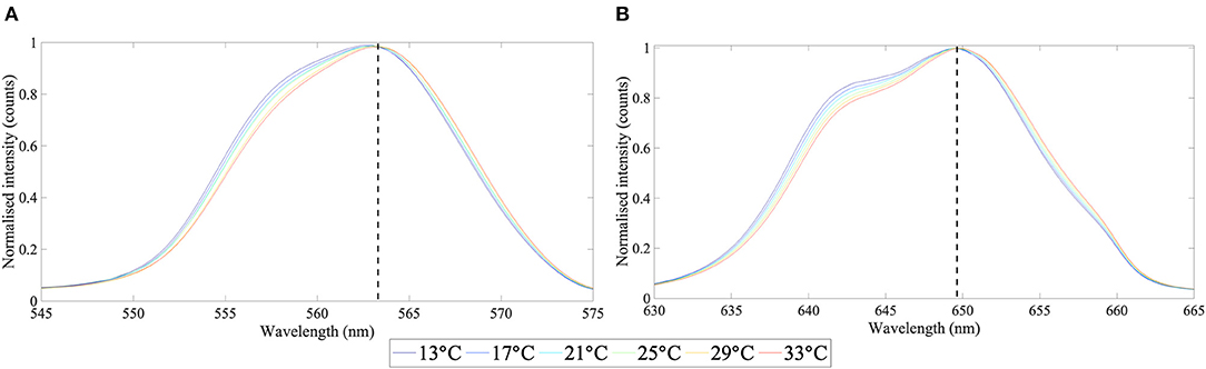
Figure 1. Temperature-dependent Raman unpolarised spectra from a Milli-Q water sample using (A) blue excitation at 473 nm (QE65000 Raman spectrometer, average sampling interval of 14 cm⁻¹ for the OH stretching band region); (B) green excitation at 532 nm (Enwave EZ-Raman spectrometer, 2 cm⁻¹ sampling interval).

Blue excitation light has not been widely used for Raman remote sensing of water temperature, and most oceanographic LIDAR methods for bathymetric measurements employ green excitation at 532 nm. Nevertheless, the use of blue lasers would be beneficial for LIDAR implementations in natural waters for the following reasons: (1) avoiding direct overlapping between the Raman peak and fluorescence from Chl-a at 680 nm (James et al., 1999; Lin, 2001); (2) Blue light has high transmission in most coastal and oceanic waters, achieving higher depths than green light (Jerlov, 1968); (3) the Raman cross-section of liquid water is inversely proportional to the wavelength of Stokes-shifted photons (Faris and Copeland, 1997); (4) wavelengths for Raman shifted photons generated by blue excitation are in the green range, undergoing lower transmission losses for returned Raman photons around 560 nm (for blue excitation) than 650 nm (for green excitation). Despite being effective in avoiding overlap with the Chl-a fluorescence peak, Raman signals scattered from blue excitation are more susceptible to overlap with DOM fluorescence. Accordingly, it is necessary to evaluate which excitation wavelength will be less likely to overlap with fluorescence from natural water constituents and provide better accuracy for Raman temperature predictions.

In this work we present a multichannel, LIDAR-compatible Raman spectrometer (RS) integrated to a 473 nm (blue) pulsed laser which is used to determine the temperature of small volumes (cuvettes) of ultrapure and natural samples. We have evaluated the effectiveness of the two-color and depolarisation temperature markers, each of which is calculated from spectral channels acquired simultaneously by the RS, in terms of sensitivity to temperature change, % error in the markers and the accuracy with which temperature can be predicted. Finally, we explore the relative merits of using blue vs. green laser excitation, with a view to understanding which source might ultimately be best for use in field measurements. This is firstly in terms of comparing the measured accuracies with those reported in de Lima Ribeiro et al. (2019b) using green excitation. Second, we use simple LIDAR equations to estimate the relative Raman returns for the cases of blue and green excitation.

Methods and Analysis

Spectrometer Design

The experimental setup for our multichannel LIDAR-compatible Raman spectrometer using a 473 nm laser is shown in Figure 2 (hereafter this will be referred as “blue multichannel RS”). Milli-Q (ultrapure) and natural water samples collected at a location inside Sydney Harbor were placed inside a temperature-controlled cuvette holder (QNW QPod2e, accuracy of ±0.2°C) and their temperature was varied from 18 to 40°C, stepping every 2°C. For natural water samples, Raman signals were acquired within a few hours of collection. Blue light produced by a linearly-polarized 473 nm pulsed laser (Nd:YAG, 5 μJ per pulse, 1.5 ns at FWHM, 5 kHz repetition rate) was collimated by lenses and coupled into the samples via a Dichroic Mirror (DM, Semrock Di02-R488, R~94% from 471 to 491 nm, T~93% between 499.8 and 900 nm). Raman-scattered photons passed through a Long Pass filter (LP, Semrock BLP01-473R, T~93% between 486 and 900 nm) in order to eliminate Rayleigh scattering, and were split into 2 beams by means of a 50/50 Beam Splitter Cube (BSC). Each beam then passed through a Band Pass filter: $B{P}_{low}^{561}$ acquiring photons at the low shift end (Semrock FF01-561/4, central wavelength at 561 nm and band pass of 8 nm at the FWHM) and $B{P}_{high}^{568}$ acquiring Raman photons at the high shift end (Semrock LL01-568, central wavelength of 568 nm and band pass of 4 nm at the FWHM). The choice of BP filters was constrained by commercial availability, and the pass band for each of these filters is indicated in Figure 3. In units of wavenumbers, the spectral widths at the FWHM were 254 cm⁻¹ for the low shift channel and 136 cm⁻¹ for the high shift channel.

FIGURE 2

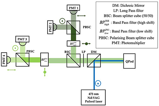
Figure 2. Experimental design of the 4-channel Raman spectrometer.

FIGURE 3

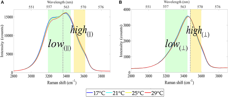
Figure 3. Band pass filter transmissions superimposed on (A) parallel and (B) perpendicularly-polarized temperature-dependent water Raman spectra.

After passing through the BP filters, each beam was divided into two polarized components by a Polarizing Beam Splitter Cube (PBSC), which were finally focused by lenses (f = 25 mm) onto fast-response photomultipliers (PMT, Hamamatsu H10721-20). The PMT gains were set around 700 V, well-below the setting for maximum gain (900 V). Signals from each channel were registered by a four-channel oscilloscope (Tektronix DPO4104B), with averaging over 512 pulses.

In order to estimate signal-to-noise ratios (SNR), acquisitions were performed with and without excitation light, with averaging over 512 pulses. SNRs were calculated for each spectral channel according to Equation 1:

$\begin{array}{ll}\begin{array}{c}SNR=\frac{\int {\text{Signal}}_{\left(\text{FWHM}\right)}}{\int {\text{Noise}}_{\left(\text{FWHM}\right)}}\end{array}& (1)\end{array}$

where ∫Signal_(FWHM) represents the integrated Raman signal pulse around the full width of half maximum (FWHM); and ∫Noise_(FWHM) refers to the integrated noise signals over the same time period.

Table 1 shows a list of information regarding each spectral channel of collection, including polarization state, band pass filter used, typical SNRs and the nomenclature which will be adopted in this paper.

TABLE 1

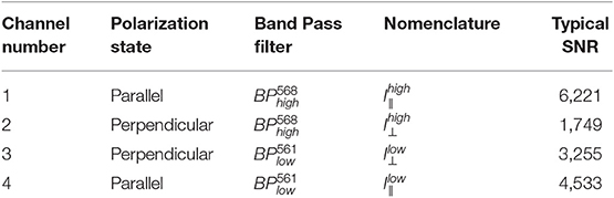
Table 1. Nomenclature adopted for each spectral channel and typical SNRs.

Temperature Markers Calculations

Each average of 512 pulses acquired by the oscilloscope was integrated in Matlab (Mathworks, R2017b) using the trapezoid method over an approximate range of 2.0 ns around the FWHM, corresponding to 10 data points (Figure 4). Raman signals corresponding to those spectral channels were used to calculate four types of temperature markers, according to Equations 2–5.

$\begin{array}{ll}\begin{array}{c}Two-color(\parallel )=\frac{I_{\parallel }^{high}}{I_{\parallel }^{low}}\end{array}& (2)\end{array}$

$\begin{array}{ll}\begin{array}{c}Two-color(\perp )=\frac{I_{\perp }^{high}}{I_{\perp }^{low}}\end{array}& (3)\end{array}$

$\begin{array}{ll}\begin{array}{c}Depolarisation(A)=\frac{I_{\perp }^{high}}{I_{\parallel }^{low}}\end{array}& (4)\end{array}$

$\begin{array}{ll}\begin{array}{c}Depolarisation(B)=\frac{I_{\perp }^{low}}{I_{\parallel }^{high}}\end{array}& (5)\end{array}$

where $I_{pol}^{xxx}$ indicates the intensity of Raman signal at a certain channel (high/low) on a given polarization state.

FIGURE 4

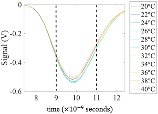
Figure 4. A typical set of signals (channel 4), recorded for different temperatures and showing the area over which the signals were integrated.

For each water sample, three independent acquisitions were performed for each temperature, hence three sets of two-color and depolarisation markers could be calculated for each temperature. Aiming to increase robustness, the markers calculated from the independent acquisitions were averaged, giving origin to a new (fourth) dataset for each temperature marker hereafter referred as the “average markers dataset.” In order to determine the uncertainties in the temperature markers, percentage errors (%) were estimated by adding the percentage uncertainties associated with SNRs calculated for each channel used in the marker calculation.

Marker Sensitivity to Temperature

Sensitivities, i.e., the % change in a marker per °C, were estimated for markers calculated for each water sample. As outlined in Artlett and Pask (2015) the use of mean-scaled temperature markers is most useful for sensitivity calculations. Those are determined by scaling each marker by the mean value of all markers within a set of temperature measurements (Equation 6). The linear model generated from the relationship between mean-scaled markers and reference temperatures provided the information necessary to estimate sensitivities for each water sample.

$\begin{array}{ll}\begin{array}{c}\text{Mean}-\text{scaled markers sensitivity}=\frac{\text{d}(\text{marker})}{\text{dT}}\frac{1}{\text{mean}(\text{marker})}\end{array}& (6)\end{array}$

Predicting Temperature Using a Single Marker

In keeping with previous studies (Artlett and Pask, 2015, 2017; de Lima Ribeiro et al., 2019b), the relationships between temperature markers and reference temperatures are found to be linear, allowing for the use of linear regression models with coefficients gradient and intercept. These coefficients were then rearranged in order to calculate a new set of temperatures dependent on the markers, hereafter called “predicted temperatures” (Equation 7).

$\begin{array}{ll}\begin{array}{c}{T}_{predicted}=\left(\text{gradient }\times \text{marker}\right)+\text{intercept}\end{array}& (7)\end{array}$

where T_predicted represents the predicted temperature estimated by a temperature marker. RMSTE values (±°C) were calculated for the predicted temperature in comparison with the reference temperature values and used as a measure of the accuracy of temperature determination by the various markers.

Linear Combination Methods: Enhancing Temperature Predictions

Our spectrometer design enabled signals to be collected from all spectral channels simultaneously, hence the four temperature markers described in Equations (2–5) each contain independent information about temperature. In de Lima Ribeiro et al. (2019b) we proposed and evaluated a multiple linear regression model, which we will call the linear combination (LC) method, combining all four markers into one model to enhance temperature predictions according to Equation 8.

$\begin{array}{l}{T}_{predicted}={\beta }_0+{\beta }_1\times two-color(\parallel )+{\beta }_2\times two-color(\perp )\\ +{\beta }_3\times depol(A)+{\beta }_4\times depol(B)+\epsilon & (8)\end{array}$

where β₀ is an independent term, β₁₋β₄ are calibration terms generated by the model and correlated with each marker and are the residual errors. LC models for the set of “average markers” were constructed for each sample analyzed in this paper.

Results and Discussion

Milli-Q Water Analysis

In this section, we explore the temperature markers calculated from Raman signals retrieved by our blue multichannel RS for an ultrapure (Milli-Q) water sample. Specifically, we consider the accuracy of temperature predictions, markers sensitivities and % errors in the temperature markers. We consider that the Raman signals acquired from the ultrapure water sample are solely due to the interactions between the excitation light and water molecules and will give rise to optimum performance of our RS. A summary with the main results found for ultrapure water analysis is shown in Table 2.

TABLE 2

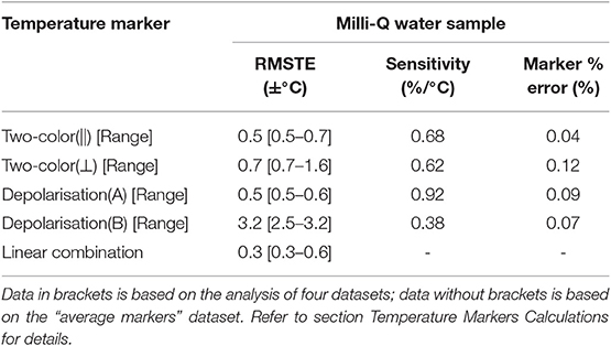
Table 2. RMSTEs (±°C), sensitivities (% change/°C), and absolute percentage errors in markers (%) for a Milli-Q water sample.

The mean-scaled value of each temperature marker is shown as a function of temperature in Figure 5. Their sensitivities extracted from the slope of each curve are summarized in Table 2.

FIGURE 5

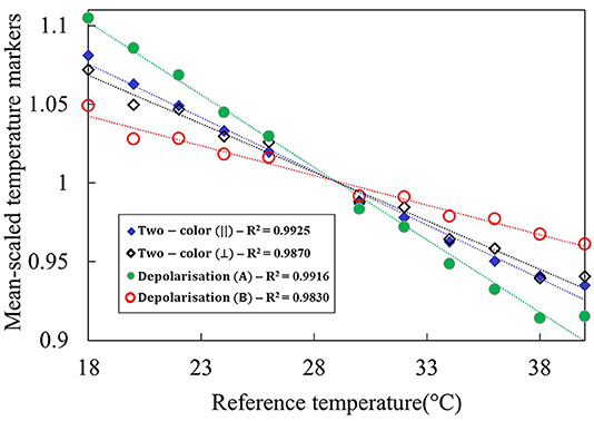
Figure 5. Mean-scaled temperature markers for Milli-Q water.

Maximum sensitivities of 0.92%/°C were found for depolarisation(A) markers, significantly higher than the second best sensitivities found for two-color(||) (0.68%/°C). Additionally, these were the markers which exhibited lowest absolute % errors [0.04% for two-color(||) and 0.09% for depolarisation(A)] and the best RMSTEs of ±0.5°C were found for both markers. Sensitivity values were generally smaller than the 1%/°C reported by the authors of Chang and Young (1972) and Leonard and Caputo (1983), however, it is necessary to consider the impact of the spectral channels widths on the final sensitivities. The authors of Artlett and Pask (2015) evaluated the trade-offs between spectral channels and sensitivities by performing simulations with unpolarized Raman signals acquired from ultrapure (Reverse-Osmosis) water samples. The mean-scaled markers sensitivities calculated from two spectral channels of 250 cm⁻¹ width exhibited values around 0.68%/°C; and sensitivities for channels widths around 150 cm⁻¹ were estimated to be around 1.03%/°C. Considering that the spectral channels used in our work had widths of 234 cm⁻¹ and 137 cm⁻¹ at the FWHM, the sensitivities found for both depolarisation(A) and two-color(||) markers were reasonably in agreement with the values proposed in Artlett and Pask (2015).

Two-color(⊥) and depolarisation(B) had inferior performance for all parameters analyzed, exhibiting lower sensitivities, higher absolute % errors and higher RMSTEs. This was particularly true for depolarisation(B) markers, with RMSTEs of ±3.2°C, sensitivities of 0.38/°C and % errors of 0.07%, indicating that the markers showed low efficiency when extracting temperature-dependent information from water Raman signals. LC methods resulted in an average improvement of 40% in RMSTEs for the Milli-Q water sample, showing it to be a valuable technique for enhancing accuracy of temperature prediction.

There is a lack of LIDAR-compatible studies in the Raman remote sensing of water temperature using blue lasers, restricting the discussion of the results from this article to comparisons with the reports of Leonard and Caputo (1983). In the occasion, the authors reported the use of a LIDAR-compatible custom-built RS integrated to a 470 nm laser (15 mJ per pulse, 2 kHz repetition rate) measuring water temperature in laboratory from depolarisation markers and finding accuracies of ±0.5°C. These were the same accuracies found for our multichannel blue RS when measuring Milli-Q water temperature from depolarisation(A) information.

In de Lima Ribeiro et al. (2019b), we reported a multichannel LIDAR-compatible RS integrated to a 532 nm excitation laser (green) which configuration was similar to our multichannel LIDAR compatible RS integrated to a 473 nm laser (blue) presented in this work. The similarities between both systems include: (1) same number of collection channels; (2) simultaneous collection of both orthogonally-polarized components of the water Raman signal; (3) same methods of calculation for temperature markers. In de Lima Ribeiro et al. (2019b), RMSTEs as low as ±0.4°C were achieved for temperature predictions from two-color(||) markers, similar to the findings in this report (±0.5°C). Regarding sensitivities, maximum values for maximum sensitivity for the green multichannel RS were 0.68%/°C, whilst sensitivities for the blue multichannel RS reached values as high as 0.92%/°C. However, comparisons between RMSTEs and sensitivities achieved in this report and the findings in de Lima Ribeiro et al. (2019b) are limited by the following factors: (1) the laser power used for excitation in the abovementioned study was five times larger than the laser power used for excitation in this study; (2) channels widths for the green multichannel RS were twice as large as the channel widths used in the blue multichannel RS; and (3) there were differences in the central wavelength relative to the Raman spectra for the blue and green RS. Both RS, blue and green, allowed for temperature predictions equal or better than ±0.5°C.

Natural Water Analyses

Natural water samples from Sydney Harbor were collected on various dates and analyzed with our blue multichannel RS. We start by acknowledging that comparisons between the results obtained for the samples are somewhat limited, considering the presence of different (unquantified) concentration of optically active components in water for each natural sample. Our intention here was to use a range of authentic natural samples in our analyses rather than “fine-tune” our methods to one particular sample.

Accuracy of temperature predictions (RMSTEs), sensitivities and % errors in the temperature markers were calculated for each natural water sample and results for the fourth dataset (“average markers”) are summarized in Table 3. The range of RMSTEs found for all datasets (1, 2, 3, and “average markers) is also indicated in the table.

TABLE 3

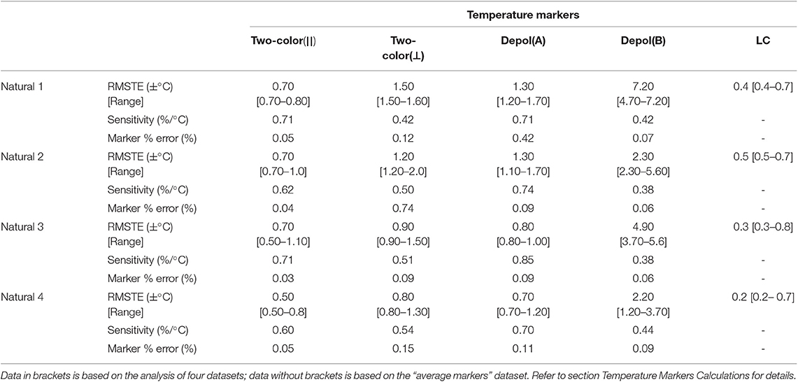
Table 3. RMSTEs (±°C), sensitivities (% change/°C), and absolute percentage errors in markers (%) for natural water sample analyzed by two-color and depolarisation markers.

We start by analyzing the temperature sensitivity for each marker in natural waters. For two-color(||), two-color(⊥) and depolarisation(A) markers, sensitivities from all natural samples were smaller of marginally greater than the ones found for ultrapure water (0.68%/°C, 0.62/°C, and 0.92%/°C, respectively). This is in agreement with the findings reported in de Lima Ribeiro et al. (2019b), where lower sensitivities were reported in natural waters due to the fluorescence of optically active constituents. Here, the main purpose of using excitation at 473 nm was avoiding Chl-a fluorescence at 680 nm, as the water Raman peak for blue excitation lies around 560 nm. However, constituents other than Chl-a exhibit fluorescence peaks around 560 nm, including DOM and other photosynthetic pigments (James et al., 1999; Lin, 1999, 2001; de Lima Ribeiro et al., 2019a), and it is virtually impossible to avoid overlapping between the water Raman peak and all possible signal sources in natural waters. In de Lima Ribeiro et al. (2019b), the presence of Chl-a fluorescence signals overlapping with the water Raman signals excited by green light (532 nm) led to higher signal counts and consequent higher SNRs, and lower % errors in the markers calculated for all-natural water sample. The same pattern was not so clearly identified in all natural water samples analyzed in the present study using blue excitation, indicating that signal counts were generally less impacted by the presence of fluorescence when using blue excitation. Comparisons between both studies, however, are limited due to the use of different natural water samples which will have particular optical characteristics. To allow for full comparison and reasoning regarding fluorescence impact in total signals, further investigations could be conducted in the future where the same natural sample is analyzed by both green (532 nm) and blue (473 nm) Raman spectrometers.

RMSTE values varied from ±0.5°C [two-color(||), natural sample 4)] to ±7.1°C [depolarisation(B), natural water sample 1]. The two-color(||) marker consistently delivered the best RMSTEs (±0.5 to ±0.7°C) for all samples. Next was the depolarisation(A) marker, which delivered RMSTEs ranging from ±0.7 to ±1.3°C. These were also the markers with highest temperature sensitivities found in this investigation. Depolarisation(B) exhibited consistent poor accuracies when predicting water temperature (RMSTEs higher than ±2.2°C) and was also the marker with lowest sensitivities in all water samples. This indicates that the temperature marker is not effectively extracting temperature information from Raman signals, and its use should be re-evaluated in future investigations.

The LC analyses resulted in average improvements in temperature accuracies of 47% when compared to the best RMSTE obtained using a single marker. Final accuracies after the LC method were equal or better than ±0.5°C for all natural water samples under investigation, indicating the method was effective extracting meaningful temperature-dependent information from multiple markers.

Considering the Relative Merits of Spectrometers Using Blue and Green Excitation

The design of our multichannel LIDAR-compatible RS using blue excitation is conceptually similar to the RS reported in de Lima Ribeiro et al. (2019b), which used a green excitation laser. In practice, the two excitation lasers differed, most notably in pulse energy, and the band pass filters defining the spectral channels also differed in regard to their width and their positions relative to the Raman band. In this section we compare the prospects for predicting water temperature using blue and green excitation, and we also evaluate the potential benefits that blue excitation might have when combined with LIDAR depth-resolved measurements. Table 4 summarizes the key characteristics of the blue and green excitation lasers used here and in de Lima Ribeiro et al. (2019b), respectively, along with the corresponding channel width, center positions and wavelength bands, as well as the key findings for temperature prediction in Milli-Q water and in natural waters.

TABLE 4

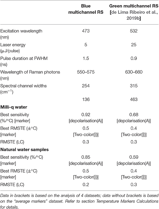
Table 4. Technical overview of two multichannel LIDAR-compatible RS integrated to 473 nm (blue) and 532 nm (green) excitation lasers.

We start our comparison by analyzing the accuracies achieved by each equipment measuring natural water temperature in the laboratory. Predictions performed by the green multichannel RS exhibited maximum accuracy of ±0.4°C, marginally higher than the RMSTEs achieved by the blue multichannel RS (±0.5°C). In both cases, these accuracies were achieved by temperature predictions using two-color(||) markers. Linear combination methods were effective in predicting temperature more accurately for both setups, with final accuracies of ±0.2°C being found for the blue RS and ±0.3°C for the green RS. These are the maximum accuracies ever reported for LIDAR-compatible Raman spectrometers predicting natural waters temperatures.

The key factors affecting RMSTEs are the intrinsic dependence of Raman spectra on temperature, and the errors and uncertainties associated with its measurement. In Milli-Q water, the measured sensitivities for the various markers reflect this dependence, plus the positions and widths of the spectral channels. According to simulations performed by Artlett and Pask (2015) for ultrapure (Reverse-Osmosis) water, an optimum trade-off between Raman signals strength and RMSTEs would be obtained for acquisition channels with spectral widths of around 200 cm⁻¹. Optimum spectral positions for such channels were explored using simulations in Artlett and Pask (2017), with the “low shift” channel central position at 3,200 cm⁻¹ and the “high shift” channel central position at 3,600 cm⁻¹. The availability of commercial Band Pass filters within these conditions is extremely limited, therefore the differences between spectral widths for channels collecting signals in the blue (254 and 136 cm⁻¹) and green (315 and 463 cm⁻¹) setups. Higher sensitivities for both setups were found for depolarisation(A) markers calculated from Raman signals scattered by Milli-Q water samples, with sensitivities of 0.92%/°C found in the blue setup and 0.59%/°C in the green. These values found in both setups are in agreement with was proposed by the simulations in Artlett and Pask (2015).

The errors and uncertainties associated with measurements performed on Milli-Q water originate from the SNR for each channel, and here the 5-times higher pulse energy of the green excitation laser, the higher Raman cross-section for blue excitation (Faris and Copeland, 1997) and the characteristics of the band pass filters all contribute. As can be seen in Table 4, despite the significant differences between the blue and green RS, the RMSTEs are remarkably similar for both cases. When it comes to natural waters, we can expect fluorescence signals arising from optically-active constituents such as DOM and photosynthetic pigments compromising the achievable RMSTE to some extent. As discussed earlier, the overlapping between the water Raman peak for this excitation and the chlorophyll-a peak at 680 nm is inevitable, reducing the accuracies that could be achieved by Raman signal analyses. Conversely, Raman photons from blue excitation have green wavelengths (550-575 nm), which exhibit good vertical transmission in water and do not overlap with the Chl-a peak; however, they are susceptible to other interactions with optically active constituents in water, such as DOM and phytoplankton.

The overlapping between the Raman peak for blue excitation and fluorescence from DOM has been previously assessed by other researchers (Dolenko et al., 2011; Vervald et al., 2015), who used Artificial Neural Networks (ANN) to solve for DOM fluorescence in water Raman spectra. The authors of Dolenko et al. (2011) created a database of Raman spectra excited by a blue laser (488 nm) acquired from water samples at different temperatures, salinities and DOM concentrations, which was used as reference by the ANN model. In the occasion, accuracies of ±0.8°C were achieved for water temperature determination, and the model was able to neglect the overlapping between DOM and Raman peaks. Later, the authors of Vervald et al. (2015) conducted laboratory investigations of natural water samples using the same ANN model, achieving accuracies of up to ±0.1°C. It is clear that ANN models are capable of minimizing the effect of the overlap between DOM fluorescence and Raman peaks acquired with blue excitation; however, this approach requires complex data manipulation and is not compatible with rapid, LIDAR methods. In de Lima Ribeiro et al. (2019a) we proposed a new technique for minimizing spectral baselines arising from fluorescence in natural waters named “correction by temperature markers.” In this method, Raman two-color markers are calculated for a “standard” water sample (i.e., a water sample without optically active constituents interacting with the excitation light) and compared with Raman markers calculated for same temperature from signals scattered by natural waters. The premise of the method is that the differences between the markers values are due to fluorescence from natural water constituents, and accuracies of up to ±0.2°C were achieved for temperature predictions in natural waters after the correction.

When it comes to considering the best excitation wavelength for combining our RS with LIDAR methods, there are additional facts to take into account. The number of Raman photons generated at a depth z and reaching the surface, N_Raman(z) can be described by Equation 9, which is based and adapted from theory presented in Leonard et al. (1979). For simplicity, we have overlooked Fresnel reflections into and out of the water and assumed solid angles of collection sufficiently small so that the Raman photons reach the surface at near-normal angles of incidence.

$\begin{array}{ll}\begin{array}{c}{N}_{Raman}(z)=N_{laser}(z)N_{scat}(z){\sigma }_{Raman}\Delta R\frac{\Omega (z)}{n^2}{T}_{\lambda 1}(z)T_{\lambda 2}(z)\end{array}& (9)\end{array}$

where N_laser(z) is the number of excitation laser photons at a given depth (z);

N_scat is the density of water molecules interacting with the excitation light (molecules/m³);

σ_Raman is the Raman scattering cross-section per molecule per steradian (m²/molecule sr);

R is the minimum vertical range resolution, determined by the laser pulse duration (m);

Ω(z) is the solid angle of collection, dependent on the diameter of the telescope or other collection optics used (steradians) at a given depth;

n is the refractive index of seawater;

T_λ1(z) and T_λ2(z) are, respectively, the vertical transmission values for the excitation and Raman wavelengths in water (m⁻¹). These are functions of $T_{\lambda }=e^{-K_{d}z}$, where K_d(λ) is the diffuse attenuation coefficient for light in water.

Modeling retrieval of Raman photons requires knowledge about the transmitter and receiver geometries and is beyond the scope of this paper. Here our purpose is to explore the relative benefit of using blue excitation, compared to green excitation. It is relatively straightforward to estimate the ratio of the expected Raman returns using blue or green excitation by considering only the terms in Equation 9 that are wavelength-dependent. The ratio is calculated assuming same pulse energy and duration for both excitation wavelengths (Equation 10).

$\begin{array}{ll}\begin{array}{c}\frac{N_{Raman}^{473}(z)}{N_{Raman}^{532}(z)}=\frac{{\lambda }^{473}{\sigma }_{Raman}^{473}{e}^{-\left(\left(K_d^{473}+K_d^{568}\right)z\right)}}{{\lambda }^{532}{\sigma }_{Raman}^{532}{e}^{-\left(\left(K_d^{532}+K_d^{660}\right)z\right)}}\end{array}& (10)\end{array}$

The top section of Table 5 provides typical values for the key LIDAR parameters (N_laser, ΔR, N_scat, σ_Raman) and the wavelength-dependent parameters used to calculate Equation 10. The bottom section of Table 5 gives the calculated 1% extinction depths for blue and green excitation and the correspondent Raman wavelengths. These are calculated for three Jerlov water types. Jerlov water type I represents oceanic clear waters, and coastal waters were represented by types 1C (clear coastal water) and 7C (turbid coastal water). Raman cross-sections σ_Raman) were calculated according to Faris and Copeland (1997) for collection channels centered at 568 nm (for blue excitation) and 660 nm (for green excitation). These “high shift” channels were chosen because attenuation increases with increasing wavelength.

TABLE 5

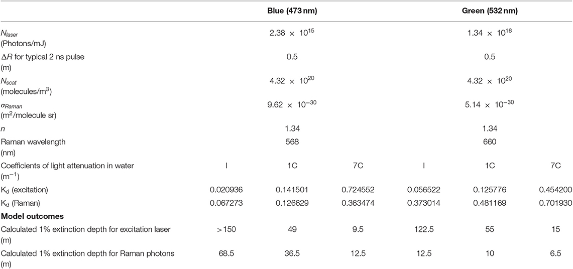
Table 5. Input parameters for LIDAR modeling and outcomes for blue and green excitation lights in Jerlov water types I, 1C and 7C.

The transmissions of the excitation laser photons and returning Raman photons in the water column were estimated using the downwelling diffuse attenuation coefficient K_d(λ). The values of K_d(λ) for Jerlov water types I, 1C and 7C were obtained from Solonenko and Mobley (2015) and interpolated for the wavelengths of interest in our study.

The depths of extinction (1% of incident light) for excitation and Raman photons varied between different Jerlov water types. For excitation light, blue light exhibited better transmission in waters type I (oceanic clear) and 1C (coastal clear); in contrast, green light had better transmission in turbid coastal waters (type 7C) in comparison with blue. For Raman returns the depths of extinction of photons at 568 nm (for blue excitation) were always >660 nm (for green excitation). Bigger differences were found in type I (factor of 5), lesser differences in type 1C (factor of 3), and small differences in type 7C (factor of 2).

Figure 6 shows the ratio of expected Raman returns under blue vs. green excitation, as a function of depth. The ratio is always >1, due to the higher Raman cross-section when blue excitation is used (factor approaching two), and the ratio increases exponentially with increasing depth. Large and very similar ratios were calculated for types I and 1C, indicating big benefits to using blue excitation, mainly due to the combination of better excitation/Raman transmissions in water. The use of blue light, however, exhibited somewhat smaller advantages for type 7C, where the much higher transmission of Raman photons (568 vs. 660 nm) is offset by the higher transmission of green excitation compared to blue. While this model is a rudimentary one, it clearly indicates the benefits of using blue excitation, predicting much greater Raman returns and therefore higher potential to determine subsurface water temperatures with reasonable accuracies. More sophisticated modeling would be required to calculate actual Raman returns and to predict the depth at which subsurface water temperature could be determined.

FIGURE 6

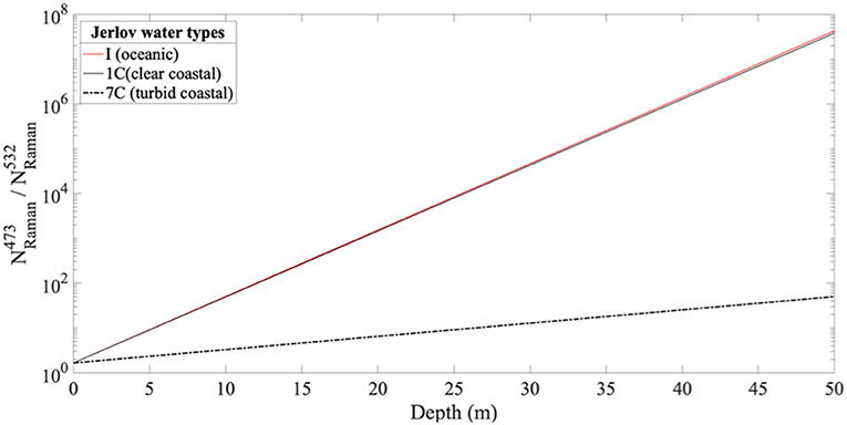
Figure 6. The ratio given in Equation 10 is plotted as a function of depth (z) for Jerlov water types: oceanic type I, and coastal types 1C and 7C.

Conclusion

We have presented the design and performance of a custom-built multichannel Raman spectrometer integrated to a 473 nm pulsed laser, employing commercial optical filters to collect polarized Raman signals at spectral regions of interest for the remote sensing of natural water temperature. Our spectrometer design is LIDAR-compatible and comprised of (1) a pulsed laser source with period ≤2 ns at the FWHM, to allow for depth resolutions better than 0.5 m; (2) collection of Raman signals at spectral regions highly sensitive to changes in temperature; (3) fast, sensitive detection by photomultipliers.

This was the first time that polarized Raman signals scattered from blue excitation (473 nm) were acquired in spectral channels for samples of natural waters and temperature was determined with accuracies as high as ±0.5°C. The simultaneous acquisition of Raman signals in four channels at different polarization states and wavelength ranges allowed for calculation of different types of temperature markers. Two-color(||) (from parallel-polarized Raman signals) and depolarisation(A) (calculated from signals of different polarization states) exhibited best performances when predicting water temperature, followed by two-color(⊥) and depolarisation(B). When all four markers were incorporated in the linear combination model, enhanced RMSTEs up to ±0.2°C were achieved. Those RMSTEs were similar to values reported in previous studies for green excitation (de Lima Ribeiro et al., 2019b).

Lastly, we have presented a simple model which predicts substantially higher Raman returns when blue excitation is used. The use of blue light is beneficial to our final goal of rapidly profiling the water column temperature by using a LIDAR-compatible system. The advantages over green light, traditionally used in oceanographic studies, include: (1) reduced spectral overlapping between Raman and fluorescence peak from chlorophyll-a at 680 nm; (2) higher Raman returns due to lower attenuation coefficients and higher Raman cross-sections.

Future work will entail field testing of the methodology presented in this paper. Particular focus needs to be given to implementing LIDAR to extract depth-resolved temperature information and strategies to mitigate the impact of fluorescence from optically active constituents.

Data Availability Statement

The datasets generated for this study are available on request to the corresponding author.

Author Contributions

AL designed and assembled the multichannel, LIDAR-compatible Raman spectrometer integrated to a 473 nm (blue) laser and conducted the experiments which led to the results presented in the manuscript. AL was responsible for performing all analyses reported in the manuscript, and also responsible for writing much of the paper and prepared the figures for publication. The Raman spectra shown in Figures 1B, 3 were acquired by C. Artlett. HP was responsible for supervising the experimental stage of this research, engaging in discussion regarding the results, and revising the manuscript.

Conflict of Interest

The authors declare that the research was conducted in the absence of any commercial or financial relationships that could be construed as a potential conflict of interest.

Acknowledgments

AL gratefully acknowledges receipt of Macquarie University iMQRES Ph.D. scholarship. HP gratefully acknowledges receipt of an Australian Research Council Future Fellowship (project number FT120100294).

References

Artlett, C. P., and Pask, H. M. (2015). Optical remote sensing of water temperature using Raman spectroscopy. Opt. Express 23:31844. doi: 10.1364/OE.23.031844

PubMed Abstract | CrossRef Full Text | Google Scholar

Artlett, C. P., and Pask, H. M. (2017). New approach to remote sensing of temperature and salinity in natural water samples. Opt. Express 25:2840. doi: 10.1364/OE.25.002840

PubMed Abstract | CrossRef Full Text | Google Scholar

Breschi, B., Cecchi, G., Pantani, L., Raimondi, V., Tirelli, D., and Valmori, G. (1992). Measurement of water column temperature by raman scattering. EARsel Adv. Remote Sens. 1, 131–134.

Google Scholar

Brewin, R. J. W., de Mora, L., Billson, O., Jackson, T., Russell, P., Brewin, T. G., et al. (2017). Evaluating operational AVHRR sea surface temperature data at the coastline using surfers. Estuar. Coast. Shelf Sci. 196, 276–289. doi: 10.1016/j.ecss.2017.07.011

CrossRef Full Text | Google Scholar

Carey, D. M., and Korenowski, G. M. (1998). Measurement of the Raman spectrum of liquid water. J. Chem. Phys. 108:2669. doi: 10.1063/1.475659

CrossRef Full Text | Google Scholar

Chang, C. H., and Young, L. A. (1972). Seawater Measurement From Raman Spectra. Technical Report for Advanced Research Projects Agency, Naval Air Development Center, document AD-753, 481. doi: 10.21236/AD0753481

CrossRef Full Text | Google Scholar

Churnside, J. H. (2008). Polarization effects on oceanographic lidar. Opt. Express 16, 1196–1207. doi: 10.1364/OE.16.001196

PubMed Abstract | CrossRef Full Text | Google Scholar

de Lima Ribeiro, A., Artlett, C., Ajani, P. A., Derkenne, C., and Pask, H. (2019a). Impact of fluorescence on Raman remote sensing of temperature in natural water samples. Opt. Express 27:22339. doi: 10.1364/OE.27.022339

PubMed Abstract | CrossRef Full Text | Google Scholar

de Lima Ribeiro, A., Artlett, C., and Pask, H. (2019b). A LIDAR-compatible, multichannel raman spectrometer for remote sensing of water temperature. Sensors 19:2933. doi: 10.3390/s19132933

PubMed Abstract | CrossRef Full Text | Google Scholar

Dickey, T. D. (2002). “A vision of oceanographic instrumentation and technologies in the early twenty-first century,” in Oceans 2020, eds J. G. Field, G. Hempl, and C. P. Summerhayes (Washington DC: Island Press), 209–254.

Google Scholar

Dolenko, T., Burikov, S., Sabirov, A., and Fadeev, V. (2011). Remote determination of temperature and salinity in presence of dissolved organic matter in natural waters using laser spectroscopy. EARSeL eProc. 10, 159–165. Available online at: http://www.eproceedings.org/static/vol10_2/10_2_dolenko1.html

Google Scholar

Faris, G. W., and Copeland, R. A. (1997). Wavelength dependence of the Raman cross section for liquid water. Appl. Opt. 36:2686. doi: 10.1364/AO.36.002686

PubMed Abstract | CrossRef Full Text | Google Scholar

Gordon, H. R. (1980). Ed Ocean Remote Sensing Using Lasers. NOAA Technical Memorandum ERL PMEL-18.

Google Scholar

Gordon, H. R. (1982). Interpretation of airborne oceanic lidar: effects of multiple scattering. Appl. Opt. 21, 2996–3001. doi: 10.1364/AO.21.002996

PubMed Abstract | CrossRef Full Text | Google Scholar

IPCC (2014). Summary for Policymakers. Geneva, Switzerland

Google Scholar

James, J. E., Lin, C. S., and Hooper, W. P. (1999). Simulation of laser-induced light emissions from water and extraction of Raman signal. J. Atmos. Ocean. Technol. 16, 394–401. doi: 10.1175/1520-0426(1999)016<0394:SOLILE>2.0.CO;2

CrossRef Full Text | Google Scholar

Jerlov, N. G. ed. (1968). Optical Oceanography, 1st Edn. Amsterdam; London, UK; New York, NY: Elsevier.

Google Scholar

Leonard, D. A., Caputo, B., and Hoge, F. E. (1979). Remote sensing of subsurface water temperature by Raman scattering. Appl. Opt. 18, 1732–1745. doi: 10.1364/AO.18.001732

PubMed Abstract | CrossRef Full Text | Google Scholar

Leonard, D. A., and Caputo, B. (1983). Raman remote sensing of the ocean mixed-layer depth. Opt. Eng. 22:223288. doi: 10.1117/12.7973107

CrossRef Full Text | Google Scholar

Lin, C. (1999). Tunable laser induced scattering from coastal water. IEEE Trans. Geosci. Remote Sens. 37, 2461–2468. doi: 10.1109/36.789642

CrossRef Full Text | Google Scholar

Lin, C. S. (2001). Characteristics of laser-induced inelastic-scattering signals from coastal waters. Remote Sens. Environ. 77, 104–111. doi: 10.1016/S0034-4257(01)00198-5

CrossRef Full Text | Google Scholar

Rees, W. G. (2001). Physical Principles of Remote Sensing, 2nd Edn. Cambridge: Cambridge University Press. doi: 10.1017/CBO9780511812903

CrossRef Full Text | Google Scholar

Solan, M., Germano, J. D., Rhoads, D. C., Smith, C., Michaud, E., Parry, D., et al. (2003). Towards a greater understanding of pattern, scale and process in marine benthic systems: a picture is worth a thousand worms. J. Exp. Mar. Bio. Ecol. 285–286, 313–338. doi: 10.1016/S0022-0981(02)00535-X

CrossRef Full Text | Google Scholar

Solonenko, M. G., and Mobley, C. D. (2015). Inherent optical properties of Jerlov water types. Appl. Opt. 54:5392. doi: 10.1364/AO.54.005392

PubMed Abstract | CrossRef Full Text | Google Scholar

Soloviev, A., and Lukas, R. (2014). The Near-Surface Layer of the Ocean. Dordrecht: Springer Netherlands. doi: 10.1007/978-94-007-7621-0

PubMed Abstract | CrossRef Full Text | Google Scholar

Vervald, A., Mazurin, E., and Plastinin, I. (2015). “Simultaneous determination of temperature and salinity of natural water by Raman spectra using artificial neural networks data analysis,” in 1st Student Workshop on Ecology and Optics of the White Sea. doi: 10.12760/02-2015-1-04

CrossRef Full Text | Google Scholar

Walrafen, G. E., Fisher, M. R., Hokmabadi, M. S., and Yang, W.-H. (1986). Temperature dependence of the low- and high-frequency Raman scattering from liquid water. J. Chem. Phys. 85, 6970–6982. doi: 10.1063/1.451384

CrossRef Full Text | Google Scholar

Whiteman, D. N., Walrafen, G. E., Yang, W. H., and Melfi, S. H. (1999). Measurement of an isosbestic point in the Raman spectrum of liquid water by use of a backscattering geometry. Appl. Opt. 38, 2614–2615. doi: 10.1364/AO.38.002614

PubMed Abstract | CrossRef Full Text | Google Scholar