True Size Matters for Conservation: A Robust Method to Determine the Size of Deep-Sea Coral Reefs Shows They Are Typically Small on Seamounts in the Southwest Pacific Ocean

Introduction

Vulnerable marine ecosystems (VME) in the deep sea are typically defined by criteria originating from international policies and actions to manage fishing impacts and conserve biodiversity (FAO, 2009). Often these criteria are based on a suite of attributes that make particular ecosystems potentially vulnerable to threatening processes, especially bottom-contact fishing; VME species have traits such as being rare, habitat-forming, fragile, functionally significant, slow to recover, or low biological productivity (Ardron et al., 2014). The criteria have mostly been applied to “indicator” species, or higher-level taxa, resulting in methods that primarily use the presence of indicator taxa to identify VME locations. These methods have become increasingly quantitative, progressing from relatively simple threshold approaches (e.g., Auster et al., 2011) to multi-criteria mapping that combines information on the vulnerability traits and abundances of target taxa with estimates of the confidence in data quality (Morato et al., 2018). Quantitative measures of indicator taxa density and spatial extent of associated habitat are viewed as the preferred technique to identify VMEs, but in the deep sea this is rarely possible using data that are independent from fisheries bycatch information (Ardron et al., 2014).

An alternative method to identifying VME locations when reliable data are lacking is using models to predict the potential suitable habitat of VME indicator taxa based on environmental variables (Vierod et al., 2014; Anderson et al., 2016b). Models are particularly useful in deep-sea settings because the areas of interest (fishery regions or bioregions) are typically large and distribution data for species and habitats sparse – a juxtaposition that is common for most of the deep ocean (Ross and Howell, 2013). The performance of habitat suitability modeling has been improved by: (i) incorporating high-resolution terrain data at regional scales (Rengstorf et al., 2013), (ii) improving faunal metrics derived from in situ video data (Rengstorf et al., 2014), (iii) validating predictions using sampling and photographic images (Anderson et al., 2016a; Rooper et al., 2016), and (iv) combining models in ensemble techniques that can improve accuracy over single models (Robert et al., 2016) and provide additional estimates of model uncertainty (Georgian et al., 2019). Habitat suitability modeling lends itself well to management applications such as conservation planning to identify potentially important habitats for reserves (Ross and Howell, 2013) and areas where managing fishery impacts could be more effective (Penney and Guinotte, 2013; Georgian et al., 2019). Despite these technical advances, most models are typically based on presence-absence or presence-only data and therefore provide no information about the abundance of VME indicator taxa. Moreover, models of presence-absence data that give the most precise predictions tend to be poorly calibrated and overconfident in their estimates (Norberg et al., 2019). The best performing models may vary according to the structure of the underlying community and how the data are collected, substantiating the approach of using multiple models and assessing the consistency between them (Norberg et al., 2019). Even where multi-criteria assessments (Morato et al., 2018) take account of abundance in point collections of fauna (e.g., fishery bycatch), there is uncertainty about how well the collections represent faunal density on the seabed because of gear selectivity and differences in the catchability of taxa. In situ photographic image data have the potential to provide abundance data on deep-sea VME taxa when the field-of-view is quantified (Althaus et al., 2009; Clark et al., 2019), and have shown that physical (sled) collections in the deep-sea are prone to underestimate faunal density – possibly by a considerable degree (Williams et al., 2015).

Habitat suitability models based on environmental data can reveal potential distributions of VME indicator taxa over data-sparse areas (Tittensor et al., 2009). Few studies have, however, attempted to define the true spatial extents of VMEs based on detailed in situ data. Quantitative in situ observations have the advantage that thresholds for defining distributions and densities of VME taxa can be determined from direct observation of deep-sea communities. Implied community or functional “ecosystem” descriptors based on observations of individual taxa can be tested for their efficacy in defining the spatial scales of VMEs, addressing directly the question of what constitutes a functional VME ecosystem unit, and how to define it based on our ecological knowledge and in situ observation.

Stony corals that build thickets or reefs and are classified as “habitat-forming,” a key attribute for VME taxa (Buhl-Mortensen et al., 2010). Reefs of the widely distributed stony corals Lophelia pertusa (Linnaeus, 1758) (currently accepted, and referred to hereafter, as Desmophyllum pertusum) and Solenosmilia variabilis Duncan, 1873 are viewed as “hot spots” of biomass and carbon-cycling on continental margins (van Oevelen et al., 2009), that harbor distinct fauna assemblages in greater abundance and diversity than those in nearby areas without corals (Henry and Roberts, 2007; Roberts et al., 2008; Althaus et al., 2009). Fine-scale mapping of coral thickets composed of D. pertusum and Madrepora oculata Linnaeus, 1758 (Vertino et al., 2010) showed the importance of distinguishing between areas where coral (live and dead) predominate from areas where corals were sparse or absent, and identifying thresholds to classify seabed cover of coral communities based on images.

In the deep sea of the southwest Pacific, S. variabilis is the dominant reef-building stony coral in terms of biomass and distribution. It is pivotal in forming habitat patches that support higher biomass and diversity on seamounts compared to adjacent slopes (Rowden et al., 2010), including distinct assemblages of some groups (e.g., ophiuroids, O’Hara et al., 2008). Reefs of this species have been mapped off New Zealand from in situ image-based data by Rowden et al. (2017) using a quantitative two stage method. First, seabed cover of coral reef and the presence of live coral, brisingids, crinoids along towed video transects was mapped to classify seabed with VME status, and then patches of reef with VME status were further assessed for the presence of live coral heads (above a pre-defined threshold) and used as input to habitat suitability models for a larger area. Despite having developed this abundance-based and high-resolution model ensemble approach Rowden et al. (2017) recognized that their method and model parameters needed to be tested in other areas.

In this paper, we apply the Rowden et al. (2017) method to an area of seamounts off southern Australia and test the consistency of results when parameters for identifying coral reef VME are changed. Our primary goal is to determine the robustness of the method to changes in these parameters and whether the method is sufficiently consistent to be recommended as a method to improve VME mapping as input to distribution models used to support conservation practice and fishery management.

Materials and Methods

Sampling Design

We test the sensitivity of Rowden et al.’s (2017) model to changes in mapping parameters, including the mechanics of a moving window used to define coral reef VMEs. Our test is based on sampling coral matrix formed predominantly by S. variabilis in a similar environment using very similar methods, but on seamounts that are topographically markedly different. Our data from Tasmania, Australia, are from the same general depth range (∼500–2000 m) as the New Zealand surveys, and represent a very similar South West Pacific (SWP) deep-sea megabenthic fauna; this has many identical and similar taxa, including VME indicator taxa such as the dominant habitat-forming stony coral, S. variabilis. The Tasmanian seamounts are, however, smaller (∼1–25 km² base size) conical mounts compared with the substantially larger (253–725 km²) guyots off New Zealand sampled by Rowden et al. (2017). Both areas have a known and continuing history of bottom trawl impacts from fisheries for orange roughy (Hoplostethus atlanticus, Collett, 1889; Tingley and Dunn, 2018), which makes them directly relevant to the FAO goal of managing both for sustainable fisheries and the protection of VMEs (FAO, 2009).

Data Collection

The study area in Australian waters lies off the east and south coasts of Tasmania (Figure 1). Data were collected during a voyage in November-December 2018 on Australia’s National Marine Facility vessel, the RV Investigator. The “Tasmanian Seamounts” area is known from a previous study of seabed habitats and megabenthos associated with some 130 small conical volcanic seamounts; the earlier study focused on trawling impact (Althaus et al., 2009) and faunal recovery (Williams et al., 2010) following commercial bottom trawling for orange roughy.

FIGURE 1

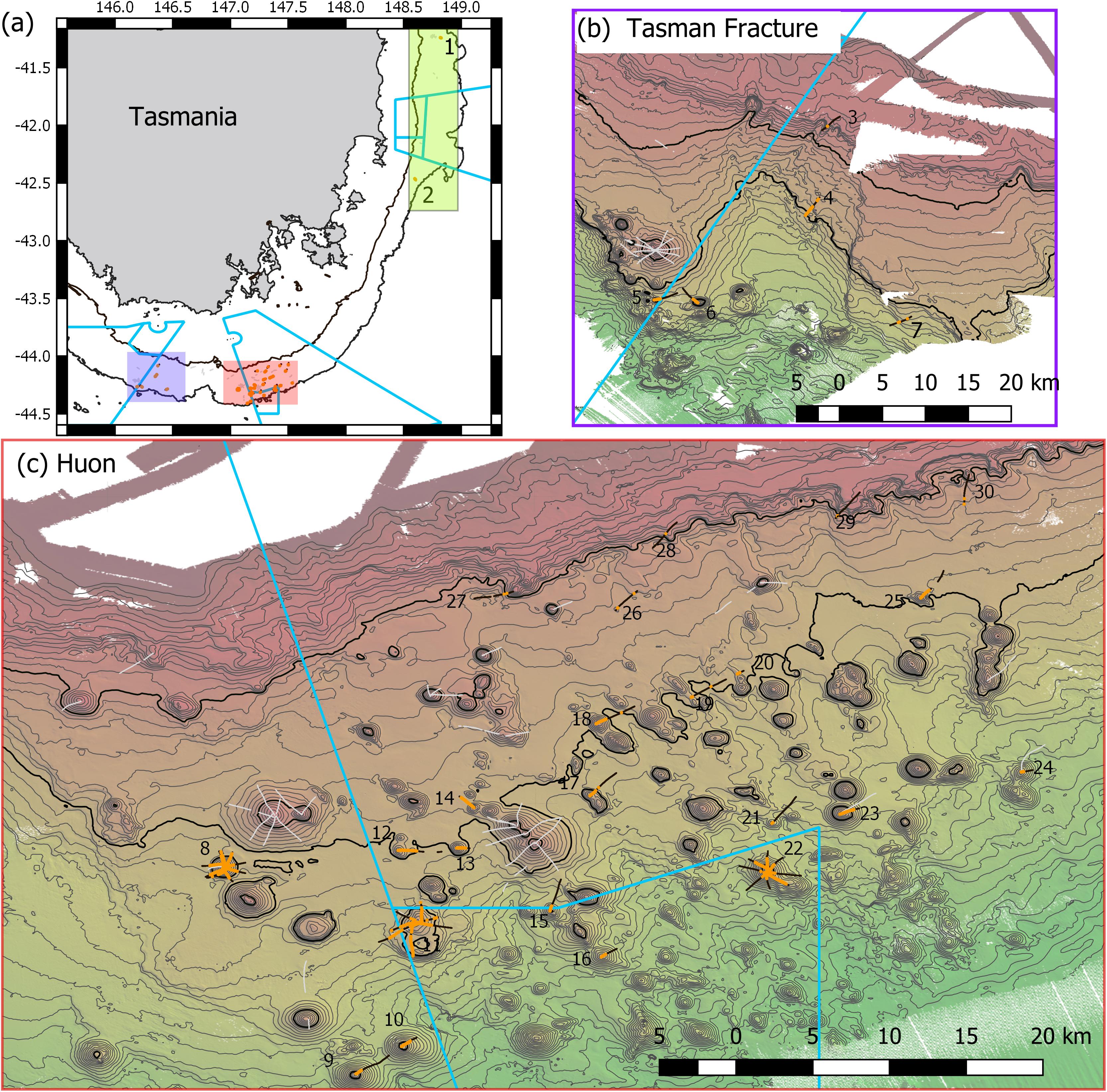
Figure 1. Maps of Tasmanian Seamounts survey area showing locations of the 30 transect sites sampled: (a) overview map showing east coast sub-area (green shaded box; sites 1 and 2) and south coast sub-areas – orange and mauve boxes; (b) south coast Tasman Fracture sub-region (sites 3–7); (c) south coast Huon sub-region (sites 8–30). Photographic transects (black lines) with distribution of the stony coral Solenosmilia variabilis matrix (live and dead) overlaid (orange); transects with fishing impacts eliminated from analysis (gray lines). Boundaries of Australian Marine Parks (blue lines); Depth contours: panel (a) 250 and 2000 m – define the limits of the survey area; panels (b,c) 50 m intervals with 950 and 1350 lines bolded.

In the present study, the extents of stony coral VMEs were estimated from image data taken by a towed camera along transects that were typically 2 km in length. Transects were located in space using a flexible spatially balanced design (Foster et al., 2020) and were of three types: (1) randomized “radial” transects on selected seamounts; (2) randomized “baseline transects” that crossed slope and seamount habitats; and (3) “ad hoc” transects that were completed during vessel transits between pre-determined sites under designs 1 and 2. The two criteria for transect selection in this analysis were: (1) that the highly dominant reef-forming stony coral S. variabilis (Figure 2) (referred to in this paper as “coral” and “coral reef”) was present along a transect, and (2) that transects had not been impacted by bottom trawling. This resulted in a total of 52 transects suitable for analysis in this study. The historical distribution of trawling effort was available from logbook data recorded by the Australian Fisheries Management Authority (AFMA) at 0.01° resolution (see methods in Althaus et al., 2009), from information provided by knowledgeable commercial fishers, and from observations during the previous studies. Most of the sites selected lie within or between the Huon and Tasman Fracture Australian Marine Parks that were closed to trawling in 2007 (Figure 1). Details of the 30 study sites are provided in Table 1.

FIGURE 2

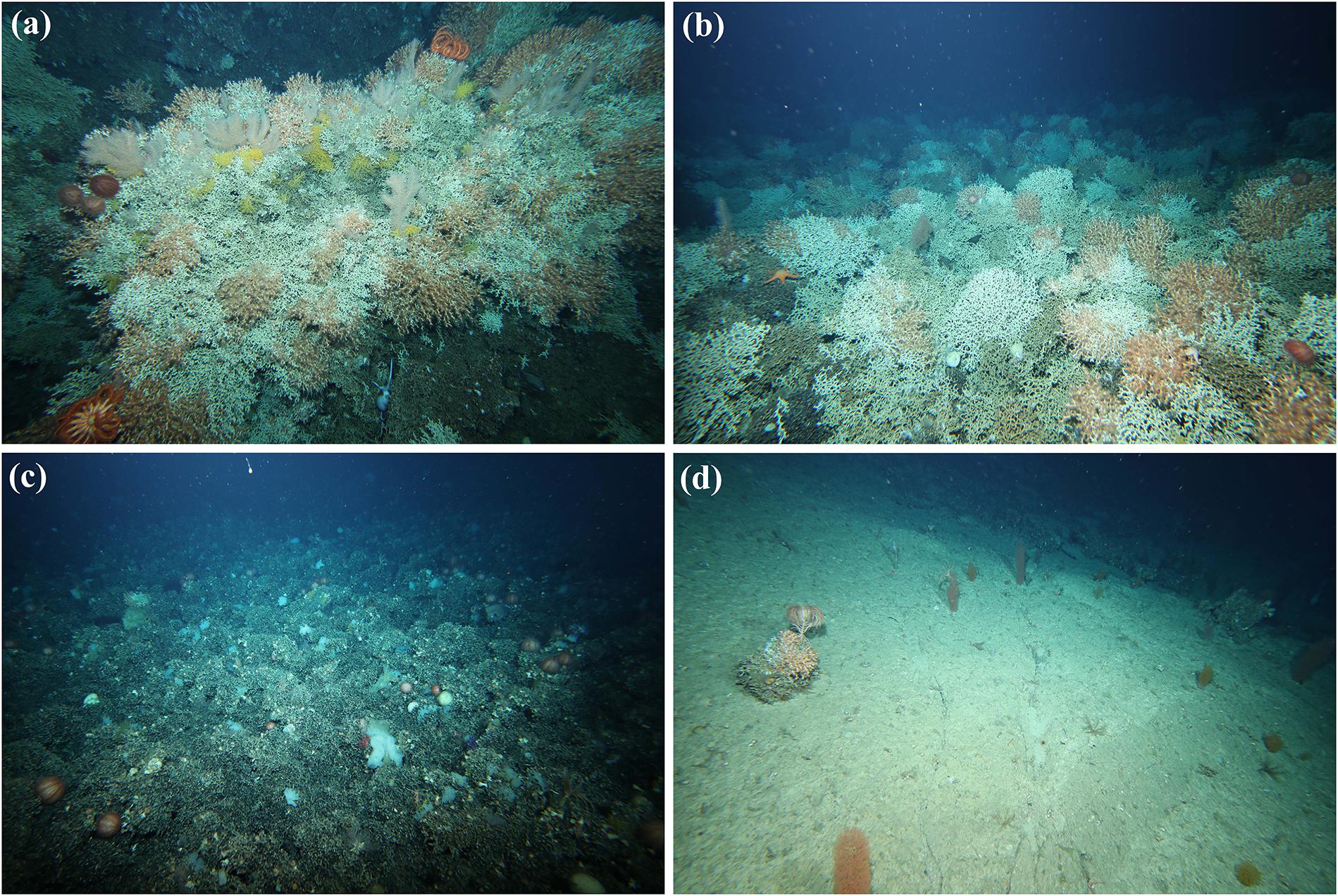
Figure 2. Examples of reef formed by the stony coral Solenosmilia variabilis on Tasmanian seamounts showing: (a,b) high % cover and many live coral heads (living polyps are orange); (c) high % cover of dead matrix with no live coral heads; (d) low % cover and isolated single live head.

TABLE 1

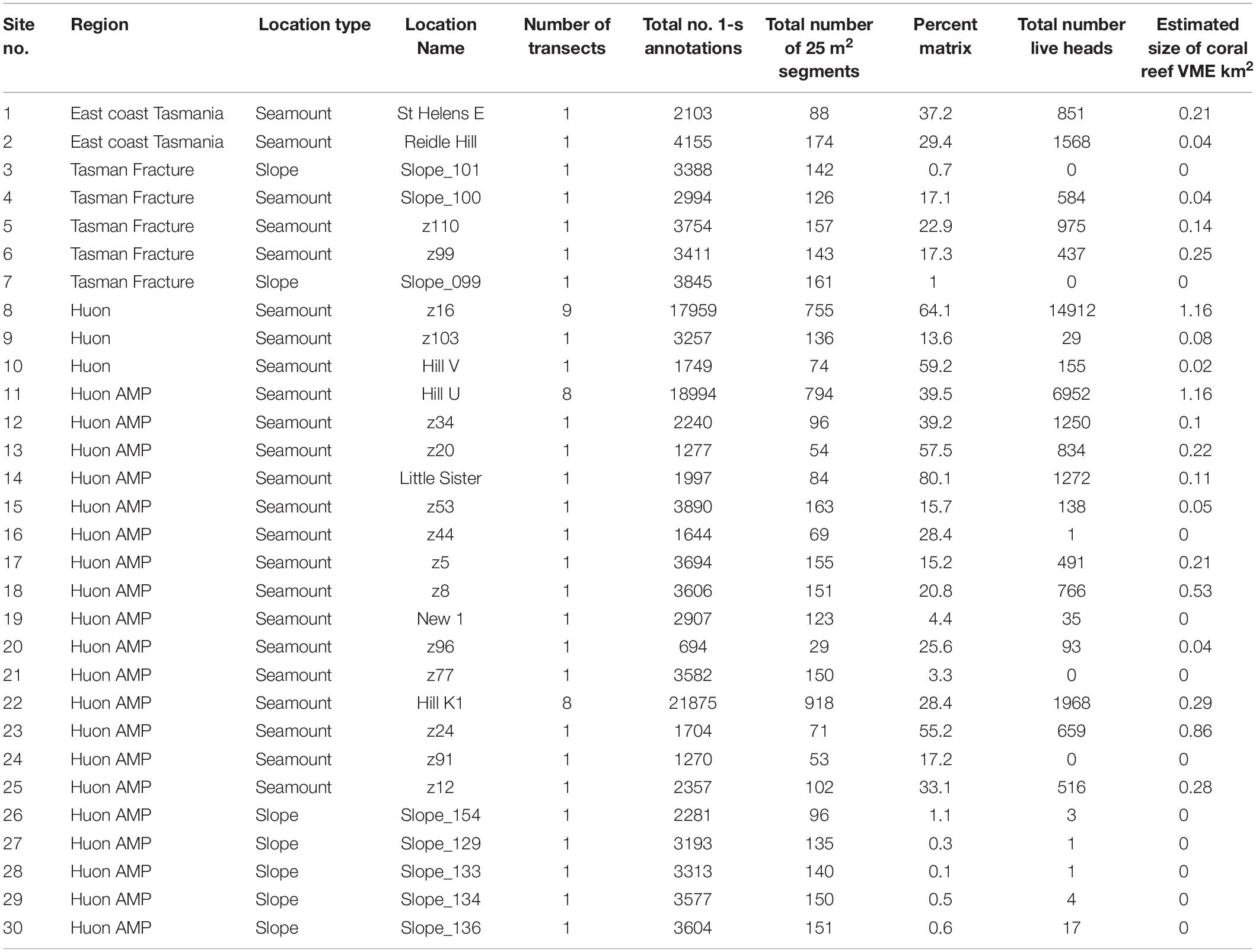
Table 1. List of sites sampled in the seamounts study area off Tasmania, Australia, detailing site reference numbers, location descriptors, and summary metrics for sample sizes and coral habitat.

The towed camera system was similar to the one used in the previous study (detailed in Althaus et al., 2009), but fitted with higher resolution cameras and a USBL that recorded with higher accuracy and frequency. In brief, a Canon EOS-1DX video camera provided continuous HD video imagery and a calibrated pair of Canon EOS-1DX Mark II still cameras provided image pairs at 5-s intervals (Marouchos et al., 2017). The system was towed at a speed of 1 knot (0.5 ms^–1) at a height of 2 m (±+0.5 m) off bottom by a pilot using camera vision transmitted back to the vessel in real-time. Video was geolocated at 1-s intervals, and all stills individually geolocated. Video was annotated for dominant substrate type on the vessel; this enabled the presence (and absence) of intact coral reef (dead or alive), and the presence of coral rubble, to be mapped along all transects. Subsequent lab-based annotation provided more detailed mapping and recorded the number of live coral heads within the portions of transects with coral reef for analysis in slow-speed replays of the video footage. Annotation was done in the Video Annotation and Reference System (VARS) developed by the Monterey Bay Aquarium Research Institute (Schlining and Jacobsen Stout, 2006) where annotations were georeferenced through linking to the processed USBL data from the camera system.

Image Data Processing and Analysis

Image data were processed in two stages following, as closely as possible, the method described by Rowden et al. (2017). In the first stage, the coral VME status of individual 12-s video segments was assessed and segments with VME habitat status were grouped into patches along transects; in the second stage, coral VME abundance was accounted for in a spatial (predictive) expansion of the patches across broader areas of the seabed.

Transect segments were classified as having “VME habitat status” if they met criteria based on the bottom cover (% by area) of seabed composed of intact coral matrix (live or dead) and the presence of live coral heads. Segments meeting these criteria (“eligible” segments) were then grouped into contiguous areas along transects (“patches”). To identify the boundary between contiguous patches and adjacent areas, which might also include isolated coral heads, segment data were processed with a moving “window” that had the effect of smoothing the patch structure over multiple segments. The effect of altering the size of this moving window was examined. Contiguous patches were identified as “coral reef VME” only if they had an abundance of live coral heads exceeding a “threshold” – a mean abundance of live heads per segment. The effect of altering this threshold was examined. The detailed data processing and analytical steps are detailed below, and the overall method is summarized schematically in Figure 3.

FIGURE 3

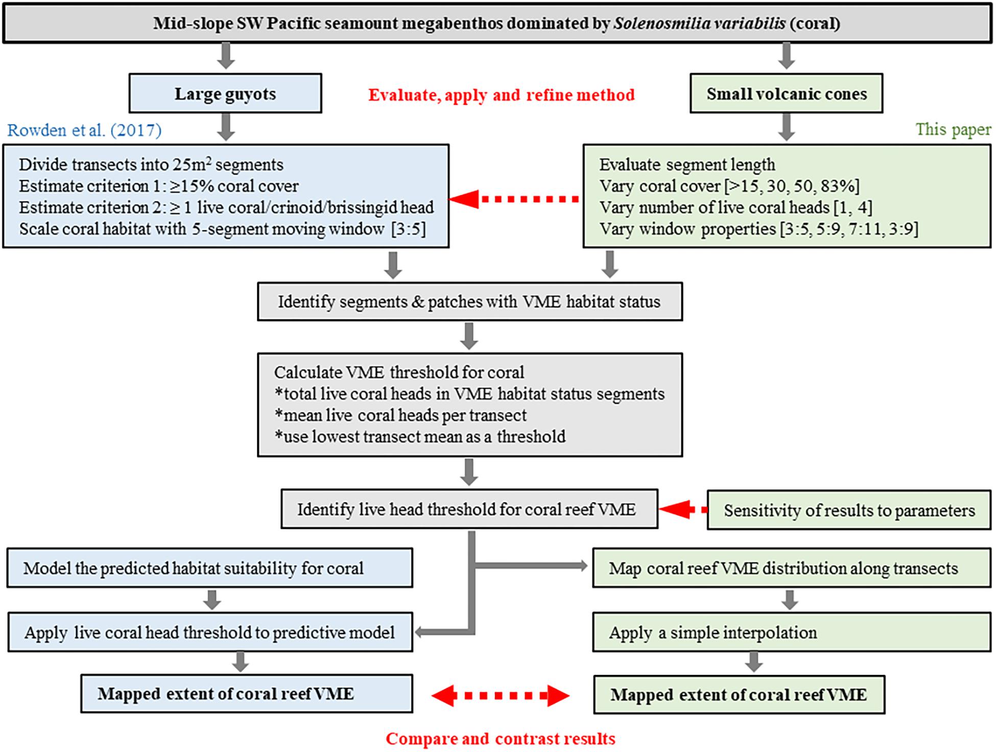
Figure 3. Schematic showing overview of process to evaluate and develop the method of Rowden et al. (2017) to spatially define coral reef VME habitat using image-derived data. The red arrows identify key phases of the process: (1) evaluate, apply and refine the method; (2) identify sensitivities to changes in methodology; (3) interpret the output for Tasmanian seamounts.

Stage 1 Analysis

Step 1 – data on % coral cover and live coral heads were aggregated to the smallest spatial unit of analysis, being a segment of ∼25 m² size (∼12 m long × 2 m plan view wide). We used elapsed time to identify the 12 m long segments along the transect path (24 × 1-s frames at an average speed of 0.5 ms^–1) together with a diminishing perspective overlay in our oblique field-of-view annotation to achieve a 2 m wide scoring corridor.

Step 2 – a segment (as defined in step one) was classified as having VME habitat status if it satisfied two criteria: (i) coral matrix covered an area of the seafloor above a particular value of % cover; and (ii) live coral heads were present (i.e., VME status of segments depended on both the cover and the occurrence of live corals).

Step 3 – A segment with VME habitat status was incorporated into a patch with VME habitat status only when it satisfied the requirement of a moving window. The requirement (rule) was for a minimum “ratio” of segments across the window to have VME habitat status, e.g., ≥3 of 5; if satisfied, the window then attributes VME habitat status to the single segment in the center of the window; each segment is sequentially classified in this way as the window moves along the transect (Figure 4).

FIGURE 4

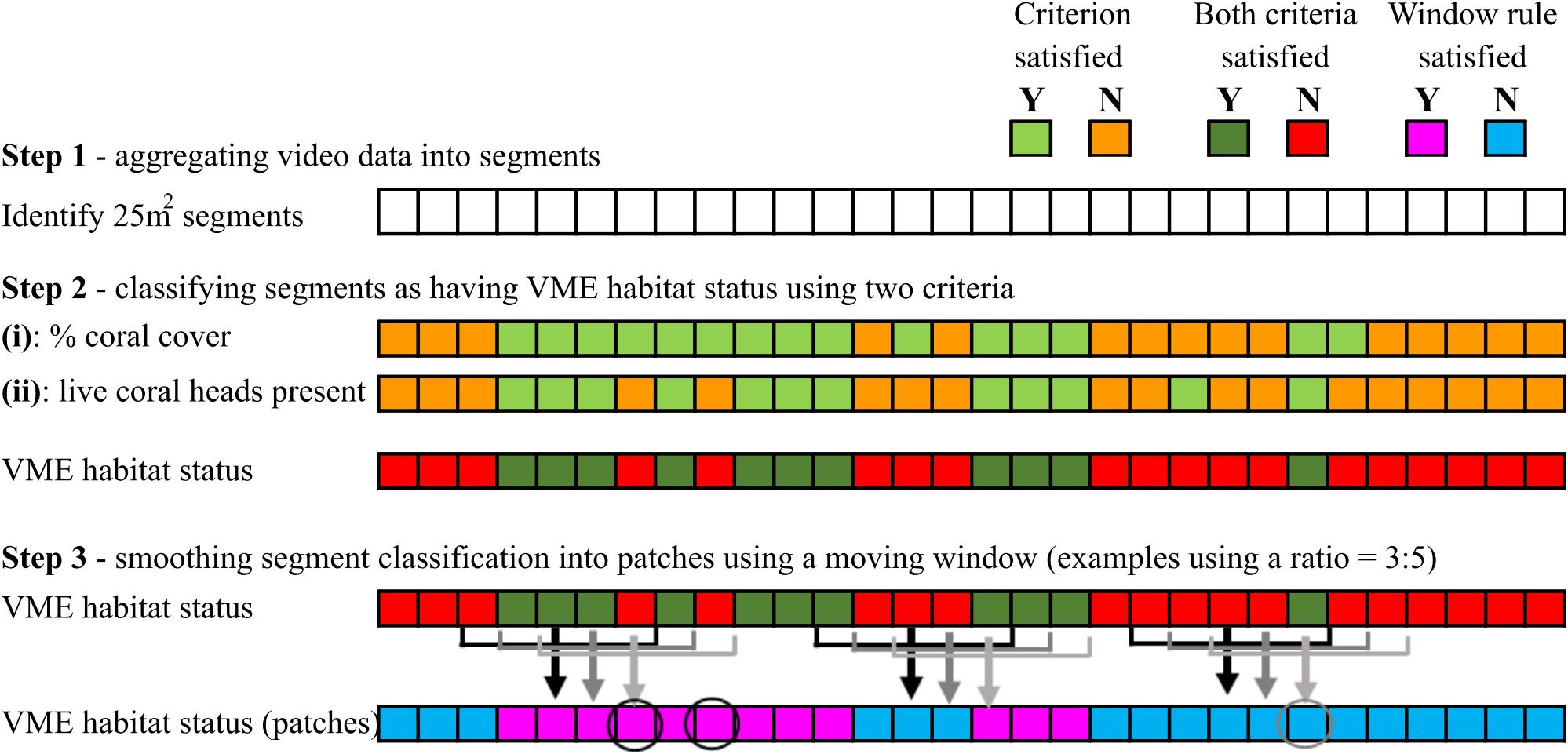
Figure 4. Schematic illustration of how VME habitat status is classified at segment scale (steps 1 and 2), and the use of a moving window to aggregate segments into patches by smoothing (step 3). In the example shown here, the smoothing rule for the moving window is for a ratio of ≥3 of 5 segments inside the window to have VME habitat status. Where the rule is satisfied, the window attributes VME habitat status to the single segment in the center of the window as it moves along the transect. Circles show examples of how smoothing may result in misclassifications.

Step 4 – Coral reef VME is attributed to segments with VME habitat status by applying a live coral head threshold. This was calculated as the number of live coral heads per segment averaged over those segments that were identified in previous analytical steps as having VME habitat status on an individual transect; the smallest value was applied as the threshold to map coral reef VMEs for the entire data set.

The stage 1 analysis (steps 1–4) is illustrated for site 8 (Seamount Z16) a symmetrical cone with simple topography in Figure 5. This shows the progression from locating coral matrix with live heads within 12 m long segments (Figure 5a), to applying the criteria for cover of coral matrix and presence of live coral heads (Figure 5b); to mapping segments with VME habitat status into patches (Figure 5c), to applying a calculated minimum threshold of number of live heads per segment (Figure 5d).

FIGURE 5

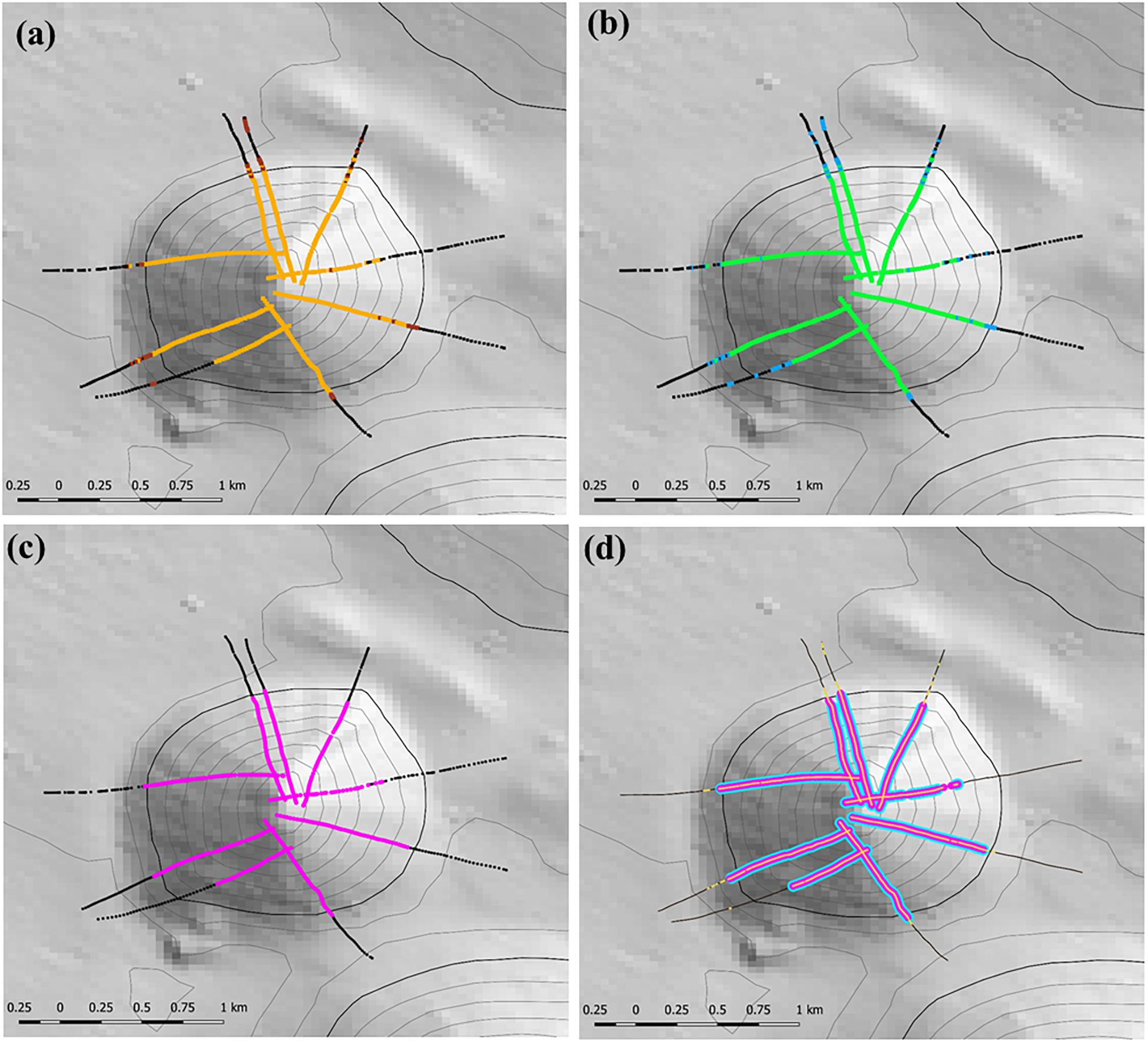
Figure 5. Illustration of the initial steps used to identify the presence and location of VME habitats at study site 8 (Seamount Z16) where camera transects were conducted; heavy depth contour = 1350 m depth: (a) step 1 – locating the presence of the matrix-forming stony coral Solenosmillia variabilis in 12 m long segments – orange = live coral, brown = dead coral; (b) step 2 – applying criteria of percentage cover and presence of live coral heads to identify segments representing VME habitat status (base-case scenario of 15% cover of coral matrix and ≥1 live coral head) – black meets neither criteria, blue meets one criterion, green meets both criteria; (c) step 3 – mapping segments with VME habitat status into patches with VME habitat status (pink) using a classification that requires ≥3 segments in a five segment moving window (3:5 ratio) to have VME habitat status; and (d) step 4 – coral reef VME (blue) is identified and mapped along patches with VME habitat status by applying a (minimum) live coral head threshold calculated across all transects. Depth contours: 50 m intervals with 1350 line bolded.

Stage 2 Analysis

Step 5 – The distribution of coral reef VME (as defined in step 4 above) was then spatially expanded, by simple extrapolation (below). We did not proceed to the development of a predictive spatial model for the entire area (e.g., Rowden et al., 2017), principally because this demanded greater resolution of physical covariates than we had available.

Scenario Testing

The classification of coral reef VME using transect data, pioneered by Rowden et al. (2017), used a single value for percentage cover (≥15%) and live coral abundance (≥1 live head), and a 5-segment moving window requiring 3 segments with VME habitat status (a 3:5 ratio) to qualify as being part of a patch with VME habitat status. We used these parameter values as a base-case scenario and examined how varying theses values (setting more conservative criteria and the properties of the moving window more and less strictly) influenced the distribution and area of seabed estimated to have VME habitat status. We first increased the percentage of % cover of coral matrix from 15% cover to 25% to match the base-case threshold of 15% over 100 m², i.e., the size of a 5-segment moving window with a 3:5 ratio rule, and then added 50 and 83% cover per segment (equivalent to 30 and 50% of a 5-segment moving window). The number of live heads was increased arbitrarily from the base-case of presence (≥1) to an abundance of ≥4 live heads. Scenarios applying different combinations of parameter values were examined for the total dataset (52 transects) and the effects measured by % change in two survey-scale metrics: (1) the number of transects in which ≥1 patch of VME habitat status was identified, and (2) the total area of seabed classified with VME habitat status combined over all transects.

We then explored how varying the length of the moving window and the number of segments required to have VME habitat status within the window (the ratio) influenced patch structure classification (length and distribution). A moving window “smooths” the patch-level classification by incorporating lone segments without VME habitat status into patches with VME habitat status and vice versa (Figure 4). Smoothing correctly classifies some lone segments but may misclassify others that occur in groups smaller than the number required by the rule for VME habitat status, e.g., groups of 2 where the rule is 3 (as for the base-case 3:5 ratio) (Figure 4).

We expected that the window’s smoothing effects – either patch-joining (creating fewer but longer patches) or patch-splitting (more but shorter patches) – would vary with window length, the required ratio of segments with VME habitat status, and the interaction of these two properties. Thus, across scenarios we aimed to provide a contrast in window length while keeping the ratio similar to base-case (3:5) and, additionally, provide a contrast in the ratio. Three scenarios were tested: (1) a longer window with similar (slightly lower) ratio = 5:9; (2) a very long window with similar (slightly higher) ratio = 7:11; and (3) a longer window and small ratio = 3:9. The effects on patch structure classification from different scenarios were examined at patch scale across transects, and at segment scale within patches. Changes across transects were measured by two transect-scale metrics: (1) the mean number of patches with VME habitat status, irrespective of patch size, across all transects with patches; and (2) the mean maximum patch size per transect. Changes in the number and distribution of segments as the result of patch-forming and patch-breaking were visualized at site 11 (Hill U), a complex seamount feature comprised of a cone with an adjacent caldera and extensive areas of rough seabed.

The basis for spatial expansion from patches with VME habitat status to areas of coral reef VME was based on calculating a live coral head threshold in the same way as Rowden et al. (2017). This was achieved by calculating the mean number of live coral heads over all segments with VME habitat status in each transect separately, and then using the minimum transect mean as the threshold for the entire data set. The Rowden et al. (2017) value (2.78) was used as the base-case. Those authors applied the live coral head threshold to predictive models that had previously mapped habitat suitability (HS) for S. variabilis on a series of large guyots; threshold-based mapping identified where coral reef VME habitat occurred within the broader areas previously identified as having some level of habitat suitability for S. variabilis. We did not have a comparable model or a suite of co-variate environmental data (notably seabed backscatter) of sufficient quality and at suitably fine spatial scales to emulate their model application. Instead, we applied a simple extrapolation of our observed VME habitat status distributions between adjacent radial transects, or around single transects. This was accomplished by extending the VME boundary, by eye, using the adjacent 50 m isobaths to generate polygons that represent the approximate estimated extent of coral reef VME. These estimates permit direct comparison of S. variabilis coral reef VME extents (sizes) in the 500–2000 m depth range on large guyots and small volcanic cones (Figure 3).

Results

Vulnerable marine ecosystems habitat status was not very sensitive to changes in key parameters used for classification (Table 2 and Figures 6, 7). Our scenario testing showed nil, negligible, or small (0–4%) changes from the base-case, either in terms of the number of transects or the area of transects identified as having VME habitat status. All effects of changing key parameters were consistently nil to very low for scenarios varying the seabed cover of corals (i.e., from a 15% base-case to 25 and 50%), and the number of live coral heads (i.e., from ≥1 base-case to ≥4 live heads).

TABLE 2

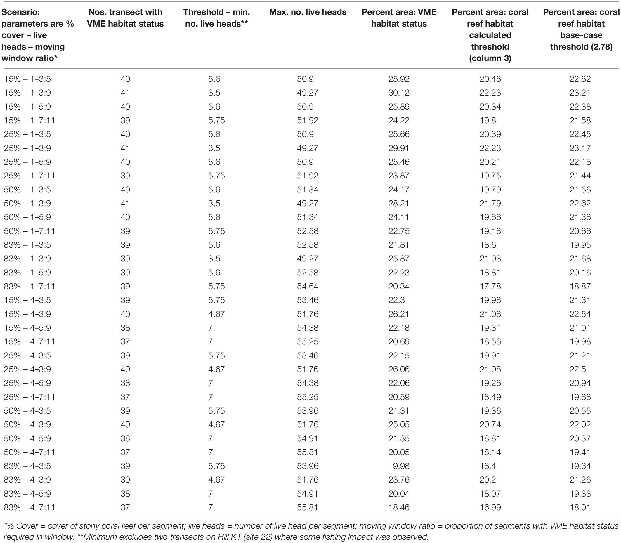
Table 2. Summary outputs from modeling scenarios used to classify habitats as having VME status; key parameters (column 1) are varied in order to test the sensitivity of the method.

FIGURE 6

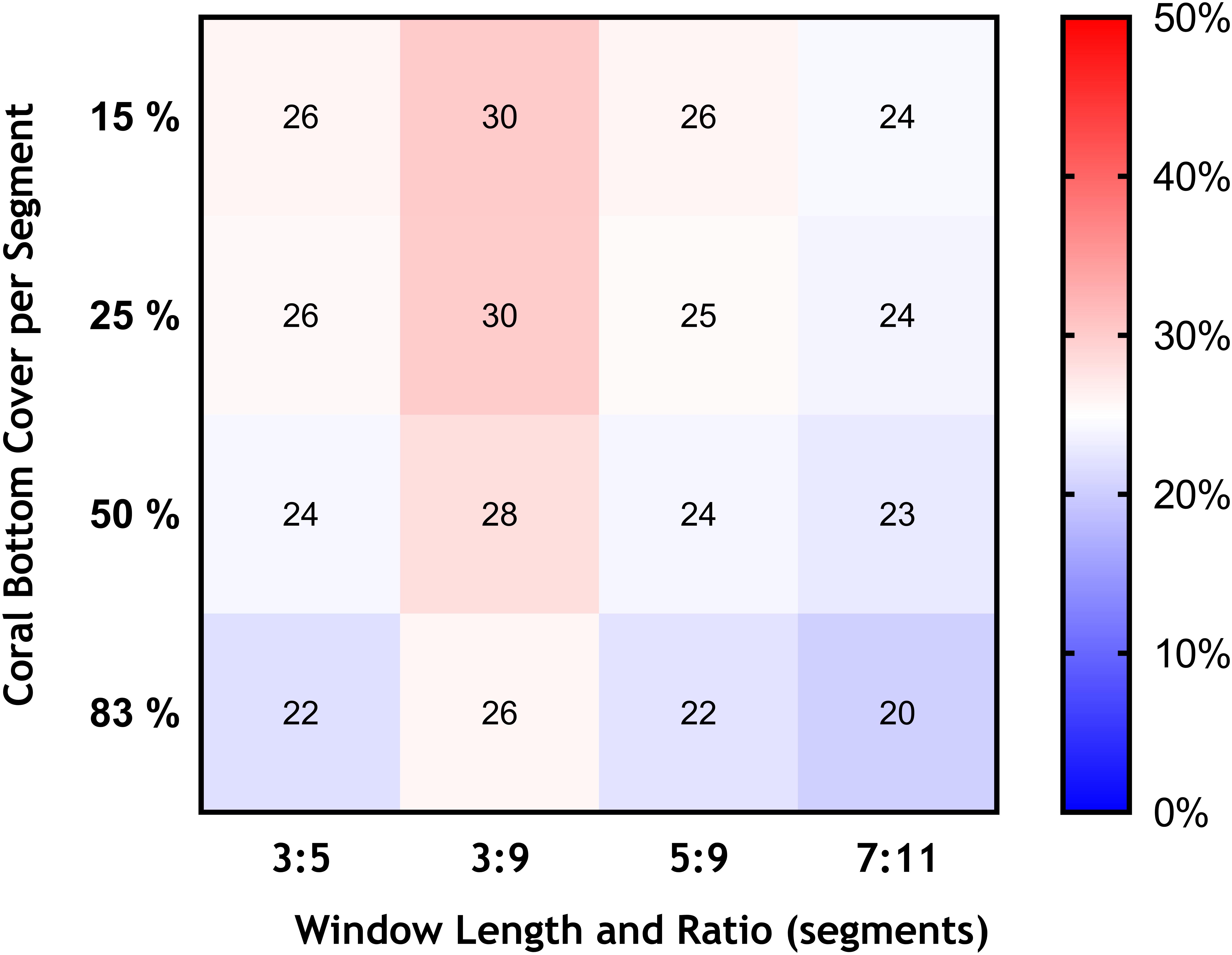
Figure 6. Effects of changing the bottom cover of coral matrix (from 15 to 83%), and the length of the moving window and ratio of VME habitat segments required within its length (3:5 base-case and 3:9, 5:9, and 7:11) in terms of the area of VME habitat identified across transects expressed as percentage of total area surveyed (color scale).

FIGURE 7

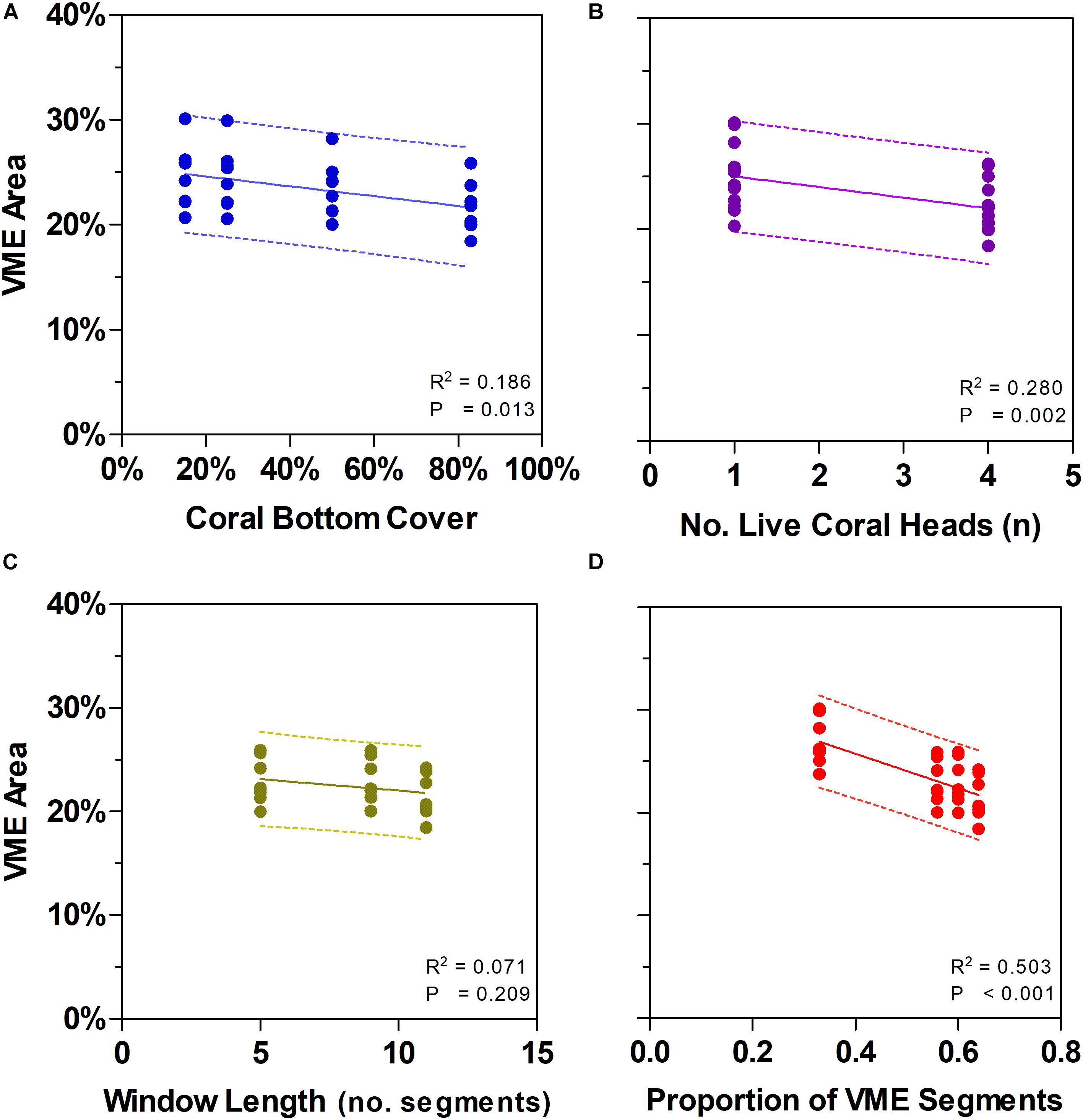
Figure 7. Effects of changing some key parameters in scenario modeling to gauge the sensitivity of a method to classify areas of deep seabed as vulnerable marine ecosystems (VME). Top row shows how changes in the criteria of bottom cover by stony corals (A) and the number of live coral heads per segment (B) influence the proportion of the sampled seabed that is classed as VME based on individual segments. Bottom row shows how segments along transect lines can be aggregated into patches using a moving window that can vary in length (C) and in the proportion of segments having to meet the criteria under (A) and (B) above inside a window (the ratio) (D). Panel (C) shows the effect of varying window length with similar ratio (∼3:5, 5:9, 7:11); panel (D) includes window with a small ratio (3:9).

Similarly, we found no substantial effects of changing the length of the moving window or the proportion of VME habitat segments required within its length (i.e., from a 3:5 ratio in the base-case to ratios of 3:9, 5:9, and 7:11) (Figure 6). A few larger changes (>4%) were observed only when we combined the largest parameter changes, being a 50 and 83% seabed cover and a ratio of 7:11 in the moving window; none, however, exceed a 6% change from the base-case. The least strict condition for the window (3:9 ratio) had the effect of increasing the computed VME area (Figure 7D).

Our scenario testing also showed small changes in patch structure from the base-case as measured by the mean number of patches with VME habitat status per transect, and the mean maximum patch size per transect (Figures 8A,B, respectively); the only sizeable difference was between the single segment (no smoothing) and all moving window scenarios. The effects of varying parameters on patch structure on individual transects are illustrated for the topographically complex site 11 (seamount “Hill U”) using selected scenarios (Supplementary Figure 1) and the four moving window ratios (3:5 base-case, 3:9, 5:9, and 7:11) (Supplementary Figure 2).

FIGURE 8

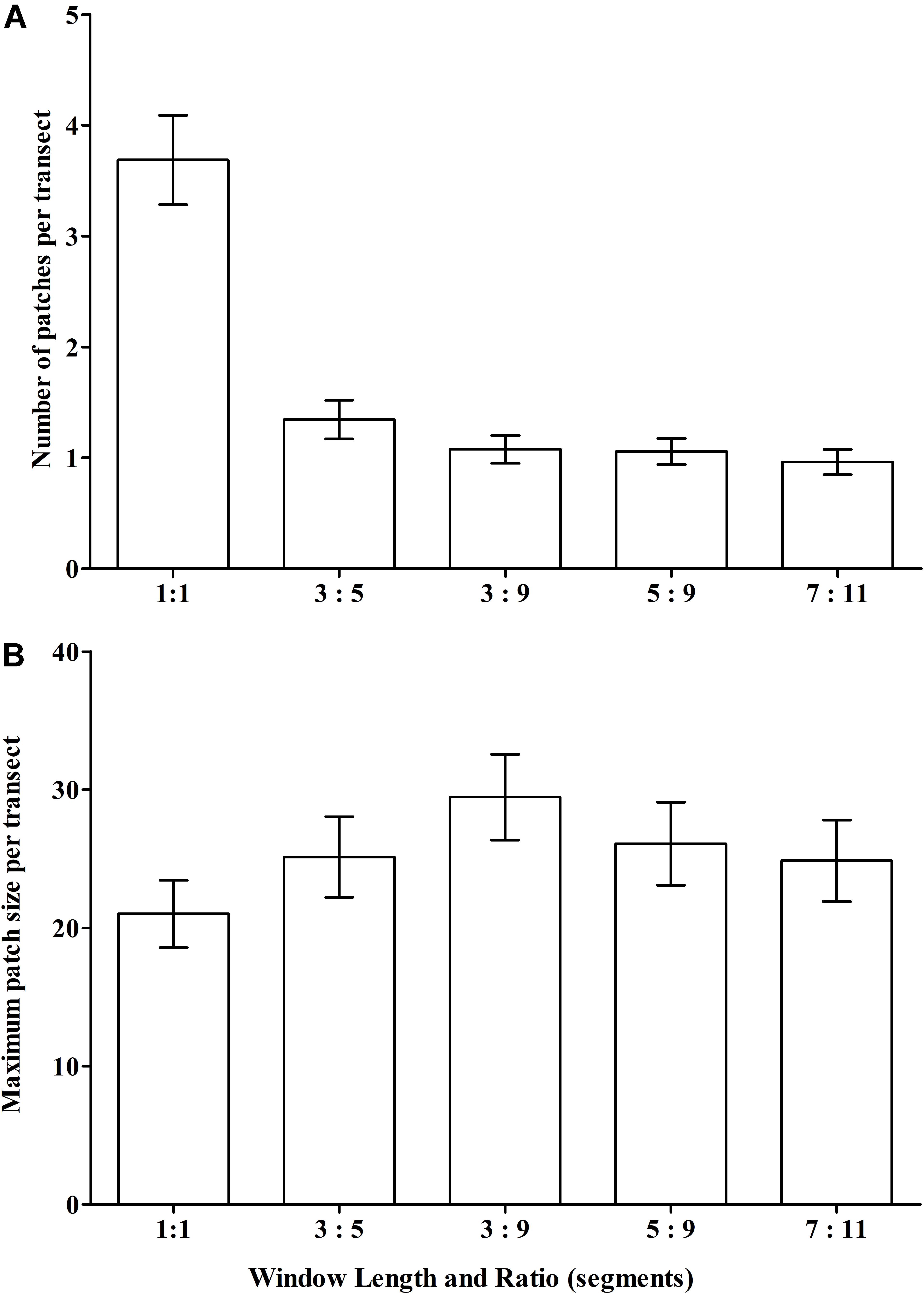
Figure 8. Sensitivity of VME classification to changes in the length (number of segments) of the moving window and the ratio of VME habitat segments required within a window to identify contiguous patches with coral VME habitat status along transects. The effects of changing the moving window ratio from base-case (3:5) is compared to single segments (unsmoothed) and ratios of 3:9, 5:9 and 7:11 as measured across all transects in terms of changes to (A) the number of patches; and (B) the maximum patch length per transect.

Any changes to patch structure that result from adding or subtracting segments with VME habitat status under different scenarios had the potential to affect the calculation of the live head threshold applied to the final spatial expansion of coral reef VMEs. Thus, in an overall exploration of methodology it was also necessary to change the live head threshold for mapping. All combinations of criteria and window properties affected the threshold value for our data, and across our scenarios this value was in a range of ∼3.5 to 7 minimum mean live heads per transect (Table 2, column 3), although with consistently lower values (3.5–4.67) when applying the least strict (3:9 ratio) moving window. Applying the Rowden et al. (2017) base-case scenario to the Tasmanian data set – 15% coral cover, 1-live coral head and a 3:5 moving window – resulted in a threshold value of 5.6 (Table 2). The effects of this higher threshold compared to the base-case (2.78) are illustrated at transect level using site 11 (Hill U) as an example (Figure 9). Compared to the base-case (Figure 9a) our higher live head threshold eliminated one deep patch of coral reef VME on transect 2 and slightly shortened patch lengths on transects 4, 6, and 7; there was also a patch break on transect 4 (Figure 9b). An increase of the % cover criterion to 25% made no observable difference (Figure 9d).

FIGURE 9

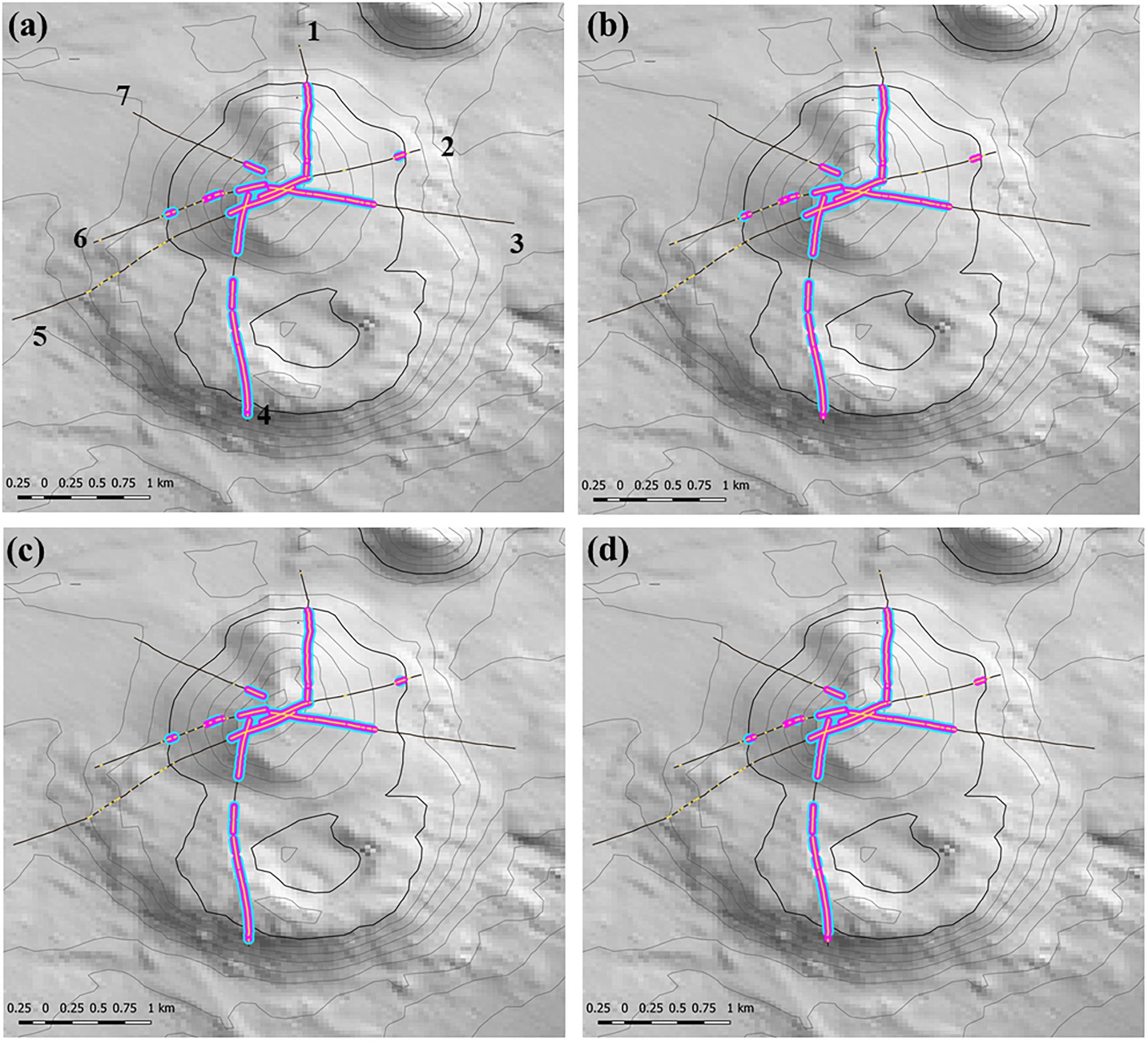
Figure 9. Transect-scale effects of changing parameters used to map coral reef VME habitat: example from site 11 (Hill U). Maps show transects (heavy black lines), the raw distribution of the matrix-forming stony coral Solenosmillia variabilis (yellow); segments defined as having VME habitat status (pink), and coral reef VME habitat (blue). Panel (a) shows transect numbers. Scenarios: (a) base-case with 2.78 live head threshold; (b) base-case with 5.6 live head threshold; (c) 25% cover and 2.78 live head threshold; (d) 25% cover and 5.6 live head threshold. Depth contours: 50 m intervals with 1350 line bolded.

A scenario of 25% cover of coral reef and 1 live head, a moving window with a ratio of 3:5, and a live head threshold of 5.6) was applied to all transects to map coral reef VME over the study area (Figure 10). The estimated size (spatial extent) of coral reef VMEs estimated from simple extrapolation showed the largest coral reef VMEs are at sites 8 (1.16 km²), 11 (1.16 km²), and 23 (0.86 km²); the smallest is at site 10 (0.02 km²) (Table 1 and Figure 11). Extrapolation appeared robust for symmetrical volcanic cones, especially where there were replicate radial transects, and supported its application to cones with single transects. Mapping on volcanic cones clearly shows a depth-related transition between coral reef VME and VME habitat around 1300–1400 m depth; contiguous intact reef extends through this depth range, but the abundance of live S. variabilis diminishes to zero and transect segments no longer meet both the % cover and live heads criteria. Mapping also clearly demonstrated where coral reef VME is absent (sites 3, 7, 16, 19, 21, 24, 26–30), even if dead or isolated small clumps of coral reef substrate were observed in the videos. Extrapolation can be done with least confidence where replicate transects show inconsistency (site 11), and on rugged rocky bottom without clear contours or morphology (sites 2, 4, 14, 20).

FIGURE 10

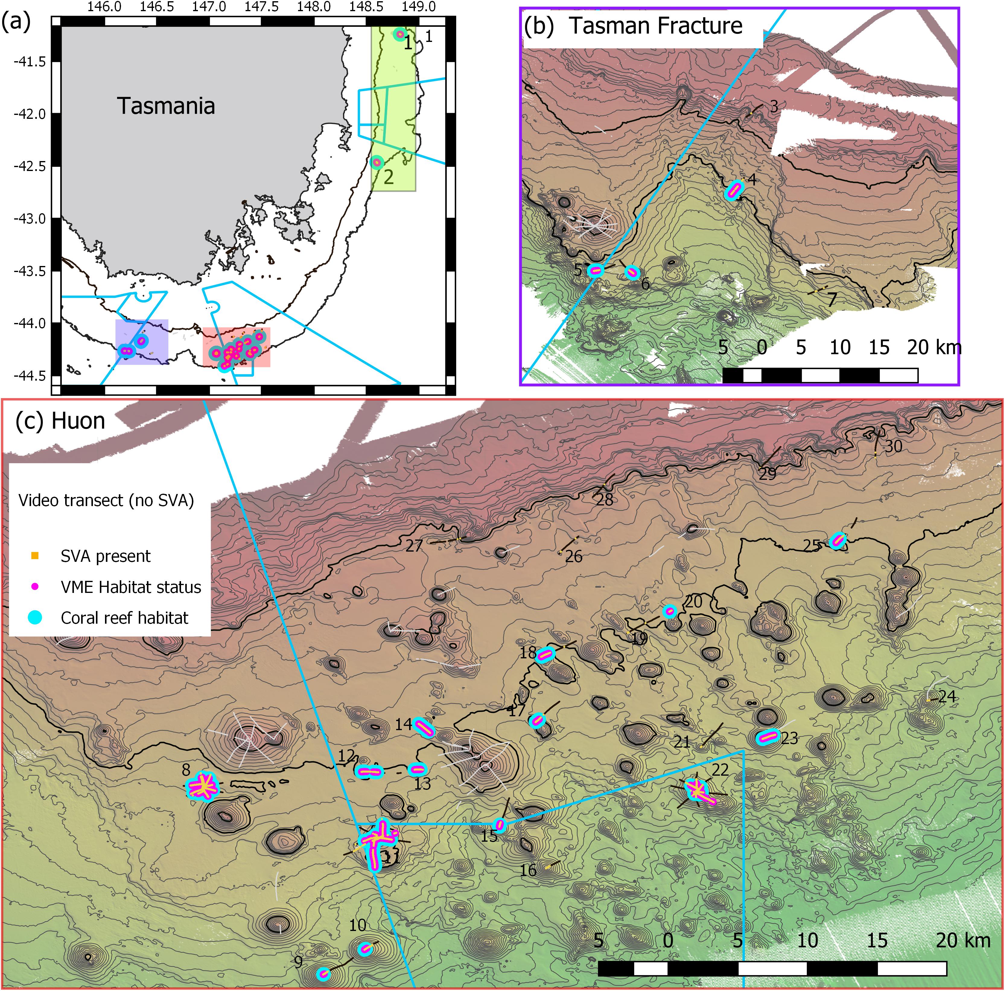
Figure 10. Distribution of Solenosmilia variabilis coral reef VME habitat (blue) across all sites. Scenario uses criteria of 25% cover of coral reef and 1 live head, a moving window with a ratio of 3:5, and a live head threshold of 5.6). Depth contours: panel (a) 250 and 2000 m – define the limits of the survey area; panels (b,c) 50 m intervals with 950 and 1350 lines bolded.

FIGURE 11

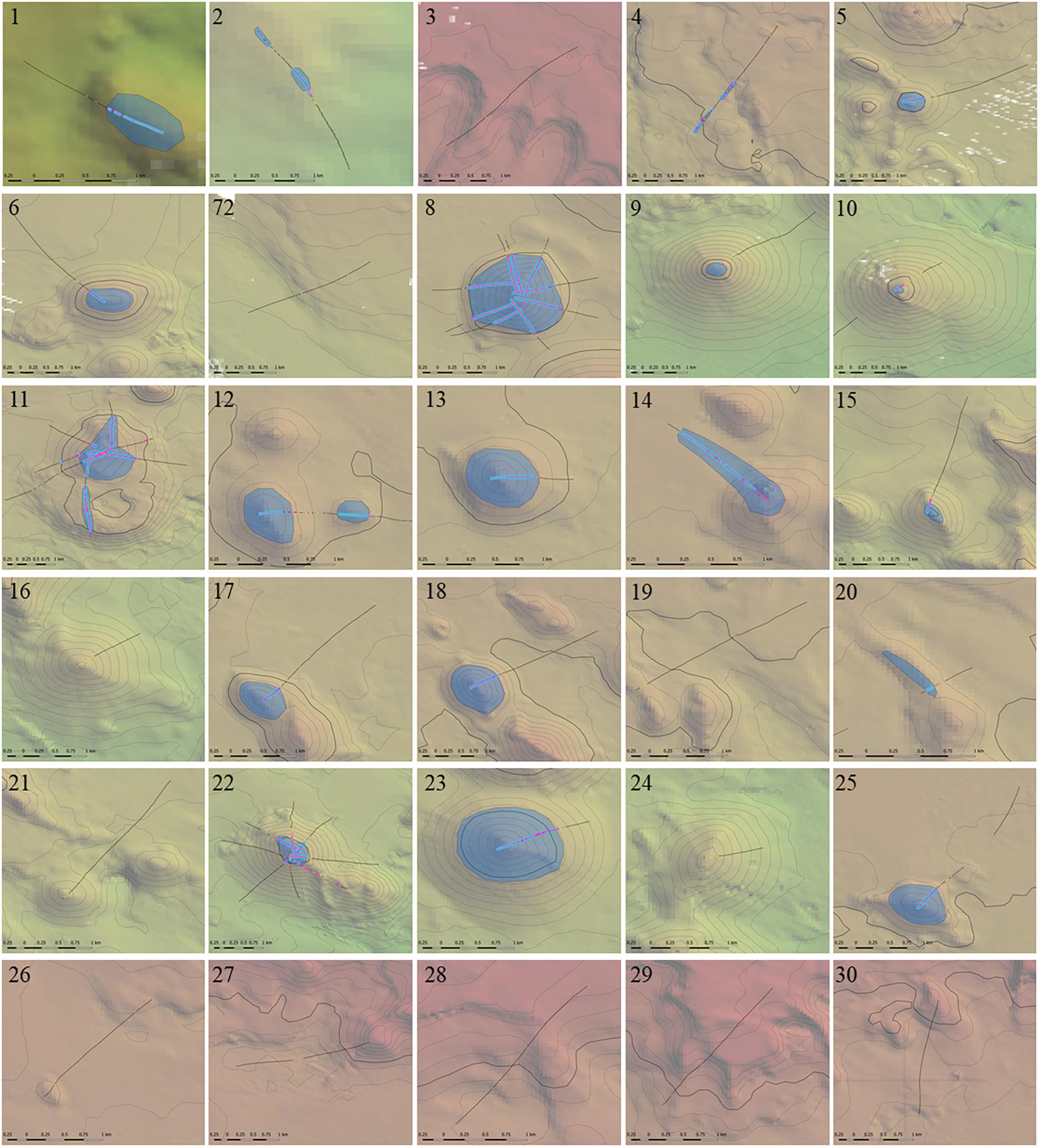
Figure 11. The estimated extent (size) of Solenosmilia variabilis coral reef VME at individual study sites extrapolated from coral reef VME mapped along transects. Mapping method as per Figure 9, with coral reef VME extent underlaid as gray polygons. Scenario uses criteria of 25% cover of coral reef and 1 live head, a moving window with a ratio of 3:5, and a live head threshold of 5.6). Depth contours: 50 m intervals with 950 and 1350 lines bolded.

Discussion

Robustness of the Method

The method of Rowden et al. (2017) to identify and map coral reef VME from image data was explored and further developed to provide an objective way of defining distributions of coral reef VME habitat formed by the stony coral S. variabilis on Tasmanian seamounts. The result successfully represented VME distribution at the feature-scale by distinguishing living coral reef from dead reef, reflecting the abundance of live coral, mapping the spatial extents of VME patches using a simple extrapolation, and by not being sensitive to a range of practical choices of parameter values chosen for VME identification from photographic transects.

The steps for identifying coral reef VME – establishing the VME habitat status of segments and combining them into patches before defining patches as coral reef VME (steps 1–4 in our method) – were robust to modest changes in parameter values or properties of the moving window. Marked differences to using the Rowden et al. (2017) base-case outcomes for classifying VME habitat status were identified only for combinations of the strictest changes to parameter values (50 and 83% cover; 4 live coral heads and an 11-segment moving window) and least-strict ratio (3:9) for the moving window. Similarly, there were only minimal differences to base-case outcomes for patch structure. Mapped scenarios for the seven transects on the example seamount (the topographically complex Hill U) showed relatively small changes in patch distributions as parameter values and window properties varied – despite many changes to the VME habitat status of individual segments. Segment-level changes affected patches mostly by shortening them; relatively few patches were eliminated, and none were created in the scenarios tested. Changes in segment status typically occurred at the ends of patches and were concentrated toward the deep distributional limit of S. variabilis around 1200–1300 m depths. The requirement to calculate a locally specific live head abundance threshold to map coral reef VME (step 4) also appeared to be robust because the threshold value calculated for the Tasmanian seamounts (5.6) was nearly double the New Zealand value (2.78) but resulted in only small changes in identified areas on the example Hill U seamount.

These patterns of low sensitivity to different analytical scenarios are partly explained by the coral reefs on Tasmanian seamounts being typically large, contiguous structures with high abundances of live coral heads. We expect there will be higher sensitivity to variation in parameters where S. variabilis reefs are more patchy. This prediction is supported by our observation that on Tasmanian seamounts, changes to VME mapping were concentrated toward the deep ends of transects where coral reefs became more fragmented. The method was applied successfully to the Louisville Seamount Chain guyots off New Zealand where coral reef VMEs are typified by smaller patches and relatively high proportions of dead coral matrix (Rowden et al., 2017). Collectively, these are positive indications for the overall robustness of the method, but its broader application needs to be substantiated by scenario testing in different environments. There are therefore no strong arguments to change the parameter values or moving window properties. We do note, however, that a 15% cover of coral reef (criterion 1) per segment needs to become 25% across the length of a 5-segment window to satisfy the minimum requirement of a 3:5 rule. Irrespective, this remains an arbitrary value that is not founded on a relationship between % cover of coral reef and its ecological significance and represents a valuable future refinement to the method.

Stage 2 of the method (step 5) requires spatial expansion of transect-based patches of coral reef VME to larger areas. Ideally this would be accomplished using a predictive modeling approach (e.g., Rowden et al., 2017), but there are demanding requirements for suitable environmental covariate data in the deep-sea context. Predictor variables need to be available for large areas but have both a native resolution that matches the spatial scale of ecological analysis (10s–100s of meters) and low uncertainty. Where abundance is a desired outcome of models, predictor variables also need to be relevant to abundance and not just presence.

Options for predictor variables in the deep sea are therefore restricted to seabed depth, derivatives of seabed bathymetry, and seabed backscatter provided by multi-beam sonar (MBS). Many of the variables derived from bathymetry are highly correlated and spatially auto-correlated, but after appropriate treatment in model data they are well suited to identifying fine-scale topography that may be informative about the fine-scale distribution of faunal abundance (Anderson et al., 2016b; Georgian et al., 2019). As well, good quality bathymetry data are typically acquired during surveys over large areas. In our area, depth makes a useful contribution to defining coral reef VME for S. variabilis because the species has a relatively narrow depth range of occurrence here (∼950–1350 m). Backscatter data have high potential for fine-scale predictive analysis because they can provide information on seabed hardness and roughness that will have often have strong correlation with the abundances of sessile benthos including corals. However, while backscatter data are collected simultaneously with bathymetry data, their quality can be insufficient for predictive mapping. We found that even after rigorous post-processing of noisy data generated by ship turns and nadir, our data were still of insufficient quality for modeling over the scale of the study area due to variations in sea state and ship direction. Carefully controlled collection of backscatter data is required to provide data sets that are fit-for-purpose for predictive modeling. Hence, we elected to estimate spatial extents of coral reef VMEs using a simple depth-based extrapolation because our initial and primary focus was at the site and feature scale. This was robust for symmetrical volcanic cones, especially where there were replicate radial transects, and supported extrapolation on cones where we had only single transects. Extrapolation was weakest where replicate transects on individual features showed inconsistency in coral reef VME distribution with depth, and on rugged rocky bottom that lacked clearly defined feature-scale topography and depth boundaries. Identifying and quantifying VME distributions on these types of locations across a regional setting will depend on whether fine-scale bathymetry-derived covariates have predictive value.

Sizes and Structure of Coral Reef VMEs on the Tasmanian Seamounts

The seabed areas identified as coral reef VME on Tasmanian seamounts were typically characterized by long contiguous patches of reef supporting highly abundant live coral heads. Coral reef VME occurred mainly on the peaks and flanks of seamounts in a depth range of approximately 950 to 1350 m; these areas were distinguished from areas where S. variabilis reef grew at low abundance (cover) and/or had no living colonies; these were mostly on the continental slope, and the deeper flanks of seamounts or near the base of seamounts (>1350 m depth) (Figure 10).

Locations of coral reef VMEs included sites where there were replicate radial transects on individual seamounts; some showed consistent and relatively uniform VME distribution on symmetrical conical features, i.e., site 8 (Seamount Z16), and others a more heterogenous distribution, particularly in areas of complex topography (e.g., over the caldera at site 11 (Hill U) and the extension of rugged bottom southwards of site 22 (Seamount K1) (Figure 11). On features where only a single transect was sampled, VME distributions were consistently mapped over the peaks and flanks of individual seamounts (Figure 11). Importantly, coral reef VME was always absent on the continental slope below the shelf edge and typically absent on flat unstructured areas of continental slope between seamounts despite some S. variabilis present as dead matrix or in small isolated clumps (Figures 2d, 10). These observations indicated that any subsequent prediction of coral reef VMEs over a broad area around Tasmania could be completed with a higher overall confidence in a predictive model. However, observations of coral reef VME away from seamounts, one associated with an extensive area of flat but rugged bottom that extended between small seamount cones at site 14 (Little Sister Seamount), another with an unusually pronounced area of raised topography on the continental margin at site 2 (Riedle Hill), and a third on the rugged bottom of the continental margin (site 4) (Figure 11), suggest the need for including fine-scale (25 m²) bathymetry-derived covariates in any model that aims to predict the distribution of coral reef VME over a broad area, and especially away from areas of high and contiguous abundance.

Coral reef VMEs on the Tasmanian seamounts are large in spatial extent (0.02–1.16 km²) when compared to those mapped on the Louisville Seamount Chain (LSC) off New Zealand (0.0006–0.0425 km²) by Rowden et al. (2017). There are also large relative differences in terms of the proportions of total areas of coral reef VME on individual seamounts. Thus, the largest and smallest estimated proportions of coral reef VME on Tasmanian seamounts are, respectively, 65% on Seamount Z16 (site 11) and 0.3% on Seamount Hill V (site 10), and correspondingly on the LSC are 0.085% on the Valerie Seamount and 0.001% on the Ghost Seamount. Thus, compared to the largest proportion of VME on an LSC seamount, the smallest and largest Tasmanian VME proportions are 3.5 and some 750 times greater. These differences in size are accompanied by differences in reef form (Figure 11 and Rowden et al., 2017, Figure 8), with coral reef VMEs on the smaller Tasmanian seamount cones composed of large contiguous “blankets” and those on the LSC guyots being more numerous, smaller and distributed patches.

How Big Is Big Enough for VME Classification?

Using the Rowden et al. (2017) method, the spatial extent of S. variabilis coral reef VME on seamounts in the Southwest Pacific Ocean was found to vary widely, from small isolated patches of 625 m² (the minimum scale of modeling) to extensive “blankets” covering 1.16 km² or more. This considerable size range raises the question of whether there are thresholds in terms of coral densities and/or reef sizes that can be considered as ecologically functional units? An answer will depend largely on the type of function considered (e.g., productivity, habitat provision, bio-geochemical processing, nursery area, refuge etc.) and the body size and mobility of associated fauna. Thus, even small reefs can be “functionally important” for small individual and/or species, particularly in a seascape setting where such feature are rare and scattered. The dominant northern hemisphere reef-builder, D. pertusum, typically creates reefs composed of live and dead coral which are numerous (e.g., ∼6000 reefs off Norway alone), round or narrow in shape and up to several 100 m in length (Buhl-Mortensen et al., 2010). A high level of biogeochemical recycling was demonstrated by Cathalot et al. (2015) at a reef of 1,767 m² in size, indicating that relatively small areas within individual reefs can make significant contributions to ecosystem processes. The localized high abundance of S. variabilis on Tasmanian seamounts was suggested by Miller and Gunasekera (2017) to be partly attributable to heavy reliance on asexual clonal reproduction for localized recruitment, with negligible dispersal of sexually produced larvae. These life history characteristics result in smaller, isolated genetic populations and a susceptibility to the effects of genetic drift, loss of genetic diversity and adaptive capacity which make the species more vulnerable to anthropogenic impacts than other reef-building coral species with relatively higher rates of sexual reproduction and more widespread dispersal – including D. pertusum. On the other hand, the minimum size for a self-sustaining population of a clonal reproducing species would be expected to be smaller than that for a population reproducing via dispersed larvae. D. pertusum also recruits through a combination of sexual and asexual reproduction but, whilst these proportions vary geographically, it has a lower proportion of clonal reproduction and therefore may be less vulnerable to impacts (Miller and Gunasekera, 2017). These observations indicate there is no single answer to the question of a minimum size for a coral reef VME, but suggest that size-based criteria need to be at least species and region specific.

For this method to be applied to other VME indicator taxa, the majority of which do not form reef-like structures, would require development of density thresholds for each taxon or group of taxa of interest. The live vs. dead criterion may be important if indicator taxa are associated with biogenic habitat, but it will be more important to assess taxa density or cover within transect segments and relate these numbers to the area over which the taxa is distributed. Applications to taxa that, compared to stony corals, have greater ranges of abundance at the spatial scales of analysis (segments and patches) and occur over much greater areas, may also benefit from exploring alternative properties for the moving window in conjunction with the density threshold.

Management Applications of Data

We anticipate that these results will assist the development of models that predict VME distributions. The use of such models has been recommended as part of the process for designing management plans to protect VMEs from fishing impacts (Ardron et al., 2014; Vierod et al., 2014), but it is acknowledged that models generally overpredict the occurrence of VMEs (Rengstorf et al., 2013; Buhl-Mortensen et al., 2019) due to not having predictors relevant to the ecological responses of VME taxa and at the relevant spatial scales. For reef-building corals there may be considerable differences between the predicted distribution of reef habitats and the broader species distribution (Howell et al., 2011). This is well demonstrated for reef-forming corals in the South Pacific Ocean by Anderson et al. (2016a) who tested model predictions with photographic field validation sampling and found that the observed frequency of corals was much lower than predicted, and correlation between observed and predicted coral distribution was moderately poor.

Recent ensemble habitat suitability modeling for a suite of VME indicator taxa in the Southwest Pacific Ocean (Georgian et al., 2019) indicated there was extensive suitable habitat (at 1 km² grid scale) for S. variabilis across much of the modeled domain. This included the Tasmanian seamount areas mapped herein, where model diagnostics indicated good performance and low uncertainty in predictions. In the Huon sub-region (Figure 10c) their model predicted at least 770 km² of suitable habitat for S. variabilis. In contrast, our analysis identified about 5 km² of coral reef VME (Figure 11 and Table 2), and, based on the restriction of coral reef VME largely to seamount peaks in 950–1350 m depths, suggests there is 106 km² of coral reef VME at most, of which some 58 km² (55%) is on seamounts where bottom trawling has occurred. Hence, our results provide evidence that the true scales of S. variabilis coral reef VMEs are relatively small when compared to regional model predictions of suitable habitat (typically smaller than a 1 km² model prediction grid cell), and much smaller than the smallest units of management interest (100s–1000s km²). While it is sometimes considered precautionary to provide maximum estimates of the spatial extent of vulnerable populations, this is only true at the initial stages of developing management measures. Once the broad area of concern has been identified, more accurate predictions are required to ensure the most important areas are protected (avoiding erroneous assumptions that vulnerable populations occur throughout the range of predicted suitable habitat), and to minimize the economic consequences of management measures. Our observations point to the need for more caution to be used in designating spatially managed areas and management tools using predictions from models, which often appear to be too optimistic. However, our evaluation of the Rowden et al. (2017) method also shows that there is a solid basis for producing accurate and reliable maps of the coral reef VMEs at the scale of individual seabed features and hence an effective and simple means to strengthen both feature-based conservation and model predictions of VME distributions at broader spatial scales.

Data Availability Statement

The data generated for this study is available on the CSIRO Data Access Portal at https://doi.org/10.25919/5e7951b49d279.

Author Contributions

AW, MC, NB, and TS designed the study. AW, MG, KM, CU, NM, MC, NB, and TS acquired the data at sea. AW, FA, MG, KM, CU, NM, and CJ acquired and processed the image-derived data. FA and AW performed the analyses. AW led the writing. All authors made substantial contributions to discussing the methods and results and revising the manuscript.

Funding

This work originates from a project that is funded, collectively, by the CSIRO Oceans and Atmosphere, Parks Australia and the Australian Government National Environmental Science Program (NESP), Marine Biodiversity Hub. Project data were collected during a voyage on Australia’s Marine National Facility Vessel, RV Investigator, funded through the Australian Government.

Conflict of Interest

The authors declare that the research was conducted in the absence of any commercial or financial relationships that could be construed as a potential conflict of interest.

Acknowledgments

We acknowledge the committees and staff of Australia’s Marine National Facility (MNF) for access to the research vessel RV Investigator, and the captain and the crew of the vessel for their hard work in making the survey successful. We also thank the sea-going staff from the MNF whose support was vital to the field collection of data. We especially thank our many colleagues from CSIRO Oceans and Atmosphere and Parks Australia, and Dr. Tiffany Sih, who helped process photographic imagery whilst at sea, and gratefully acknowledge the many other engineering, technical and administrative staff at CSIRO who contributed in various ways to supporting the project that provided the data for this manuscript. In particular, for the design and fabrication of the camera platform, and for maintaining and piloting the system at sea, we thank Matt Sherlock, Jeff Cordell, Karl Forcey, and Aaron Tyndall, and for advice and assistance with various aspects data preparation and survey design we are indebted to Scott Foster, Amy Nau and Jasmine Bursic (CSIRO), and Jan Jansen and Vanessa Lucieer (University of Tasmania). Finally, we thank staff from the IT and Data Centre at CSIRO, notably Pamela Brodie and Peter Shanks, made invaluable contributions to handling and processing the image data sets.

Supplementary Material

The Supplementary Material for this article can be found online at: https://www.frontiersin.org/articles/10.3389/fmars.2020.00187/full#supplementary-material

References

Althaus, F., Williams, A., Schlacher, T. A., Kloser, R. J., Green, M. A., Barker, B. A., et al. (2009). Impacts of bottom trawling on deep-coral ecosystems of seamounts are long-lasting. Mar. Ecol. Prog. Ser. 397, 279–294. doi: 10.3354/meps08248

CrossRef Full Text | Google Scholar

Anderson, O. F., Guinotte, J. M., Rowden, A. A., Clark, M. R., Mormede, S., Davies, A. J., et al. (2016a). Field validation of habitat suitability models for vulnerable marine ecosystems in the South Pacific Ocean: implications for the use of broad-scale models in fisheries management. Ocean Coast. Manag. 120, 110–126. doi: 10.1016/j.ocecoaman.2015.11.025

CrossRef Full Text | Google Scholar

Anderson, O. F., Guinotte, J. M., Rowden, A. A., Tracey, D. M., Mackey, K. A., and Clark, M. R. (2016b). Habitat suitability models for predicting the occurrence of vulnerable marine ecosystems in the seas around New Zealand Deep sea research part I. Oceanogr. Res. Pap. 115, 265–292. doi: 10.1016/j.dsr.2016.07.006

CrossRef Full Text | Google Scholar

Ardron, J. A., Clark, M. R., Penney, A. J., Hourigan, T. F., Rowden, A. A., Dunstan, P. K., et al. (2014). A systematic approach towards the identification and protection of vulnerable marine ecosystems. Mar. Policy 49, 146–154. doi: 10.1016/j.marpol.2013.11.017

CrossRef Full Text | Google Scholar

Auster, P. J., Gjerde, K., Heupel, E., Watling, L., Grehan, A., and Rogers, A. D. (2011). Definition and detection of vulnerable marine ecosystems on the high seas: problems with the “move-on” rule Ices. J. Mar. Sci. 68, 254–264. doi: 10.1093/icesjms/fsq074

CrossRef Full Text | Google Scholar

Buhl-Mortensen, L., Burgos, J. M., Steingrund, P., Buhl-Mortensen, P., Ólafsdóttir, S. H., and Ragnarsson, S. (2019). Vulnerable Marine Ecosystems (VME): Coral and Sponge VMEs in Arctic and Sub-arctic Waters - Distribution and Threats. Rosendahls: Nordic Council of Ministers, 155.

Google Scholar

Buhl-Mortensen, L., Vanreusel, A., Gooday, A. J., Levin, L. A., Priede, I. G., Buhl-Mortensen, P., et al. (2010). Biological structures as a source of habitat heterogeneity and biodiversity on the deep ocean margins. Mar. Ecol. 31, 21–50. doi: 10.1111/j.1439-0485.2010.00359.x

CrossRef Full Text | Google Scholar

Cathalot, C., Van Oevelen, D., Cox, T. J. S., Kutti, T., Lavaleye, M., Duineveld, G., et al. (2015). Cold-water coral reefs and adjacent sponge grounds: hotspots of benthic respiration and organic carbon cycling in the deep sea. Front. Mar. Sci. 2:37. doi: 10.3389/fmars.2015.00037

CrossRef Full Text | Google Scholar

Clark, M. R., Bowden, D. A., Rowden, A. A., and Stewart, R. (2019). little evidence of benthic community resilience to bottom trawling on seamounts after 15 years. Front. Mar. Sci. 6:63. doi: 10.3389/fmars.2019.00063

CrossRef Full Text | Google Scholar

FAO (2009). “International guidelines for the management of deep-sea fisheries in the high Seas,” in Food and Agricultural Organisation of the United Nations, Rome: FAO, 73.

Google Scholar

Foster, S. D., Hosack, G., Monk, J., Lawrence, E., Barrett, N., Williams, A., et al. (2020). Spatially-balanced designs for transect-based surveys. Methods Ecol. Evol. 11, 95–105. doi: 10.1111/2041-210X.13321

CrossRef Full Text | Google Scholar

Georgian, S. E., Anderson, O. F., and Rowden, A. A. (2019). Ensemble habitat suitability modeling of vulnerable marine ecosystem indicator taxa to inform deep-sea fisheries management in the South Pacific Ocean. Fish. Res. 211, 256–274. doi: 10.1016/j.fishres.2018.11.020

CrossRef Full Text | Google Scholar

Henry, L. A., and Roberts, J. M. (2007). Biodiversity and ecological composition of macrobenthos on cold-water coral mounds and adjacent off-mound habitat in the bathyal Porcupine Seabight. NE Atlantic. Deep Sea Re.s I 54, 654–672. doi: 10.1016/j.dsr.2007.01.005

CrossRef Full Text | Google Scholar

Howell, K. L., Holt, R., Endrino, I. P., and Stewart, H. (2011). When the species is also a habitat: comparing the predictively modelled distributions of Lophelia pertusa and the reef habitat it forms. Biol. Conserv. 144, 2656–2665. doi: 10.1016/j.biocon.2011.07.025

CrossRef Full Text | Google Scholar

Marouchos, A., Sherlock, M., Filisetti, A., and Williams, A. (2017). “Underwater imaging on self-contained tethered systems,” in IEEE Oceans Anchorage, Anchorage, 18–21.

Google Scholar

Miller, K. J., and Gunasekera, R. M. (2017). A comparison of genetic connectivity in two deep sea corals to examine whether seamounts are isolated islands or stepping stones for dispersal. Nat. Sci. Rep. 7:46103.

Google Scholar

Morato, T., Pham, C. K., Pinto, C., Golding, N., Ardron, J. A., Muñoz, D. P., et al. (2018). A multi criteria assessment method for identifying vulnerable marine ecosystems in the north-east Atlantic. Front. Ma. Sci. 5:460. doi: 10.3389/fmars.2018.00460

CrossRef Full Text | Google Scholar

Norberg, A., Abrego, N., Blanchet, F. G., Adler, F. R., Anderson, B. J., Anttila, J., et al. (2019). A comprehensive evaluation of predictive performance of 33 species distribution models at species and community levels. Ecol. Monogr. 89:e01370.

Google Scholar

O’Hara, T. D., Rowden, A. A., and Williams, A. (2008). Cold-water coral habitats on seamounts: do they have a specialist fauna? Divers. Distrib. 14, 925–934. doi: 10.1111/j.1472-4642.2008.00495.x

CrossRef Full Text | Google Scholar

Penney, A. J., and Guinotte, J. M. (2013). Evaluation of New Zealand’s high-seas bottom trawl closures using predictive habitat models and quantitative risk assessment. PLoS One 8:e82273. doi: 10.1371/journal.pone.0082273

PubMed Abstract | CrossRef Full Text | Google Scholar

Rengstorf, A. M., Mohn, C., Brown, C., Wisz, M. S., and Grehan, A. J. (2014). Predicting the distribution of deep-sea vulnerable marine ecosystems using high-resolution data: considerations and novel approaches Deep Sea Research Part I. Oceanogr. Res. Pap. 93, 72–82. doi: 10.1016/j.dsr.2014.07.007

CrossRef Full Text | Google Scholar

Rengstorf, A. M., Yesson, C., Brown, C., and Grehan, A. J. (2013). High-resolution habitat suitability modelling can improve conservation of vulnerable marine ecosystems in the deep sea. J. Biogeogr. 40, 1702–1714. doi: 10.1111/jbi.12123

CrossRef Full Text | Google Scholar

Robert, K., Jones, D. O. B., Roberts, J. M., and Huvenne, V. A. I. (2016). Improving predictive mapping of deep-water habitats: considering multiple model outputs and ensemble techniques Deep Sea Research Part I. Oceanogr. Res. Pap. 113, 80–89. doi: 10.1016/j.dsr.2016.04.008

CrossRef Full Text | Google Scholar

Roberts, J. M., Henry, L. A., Long, D., and Hartley, J. P. (2008). Cold-water coral reef frameworks, megafauna communities and evidence for coral carbonate mounds on the Hatton Bank, north east Atlantic. Facies 54, 297–316. doi: 10.1007/s10347-008-0140-x

CrossRef Full Text | Google Scholar

Rooper, C. N., Sigler, M. F., Goddard, P., Malecha, P., Towler, R., Williams, K., et al. (2016). Validation and improvement of species distribution models for structure-forming invertebrates in the eastern Bering Sea with an independent survey. Mar. Ecol. Prog. Ser. 551, 117–130. doi: 10.3354/meps11703

CrossRef Full Text | Google Scholar

Ross, R. E., and Howell, K. L. (2013). Use of predictive habitat modelling to assess the distribution and extent of the current protection of ‘listed’ deep-sea habitats. Divers. Distrib. 19, 433–445. doi: 10.1111/ddi.12010

CrossRef Full Text | Google Scholar

Rowden, A. A., Anderson, O. F., Georgian, S. E., Bowden, D. A., Clark, M. R., Pallentin, A., et al. (2017). High-resolution habitat suitability models for the conservation and management of vulnerable marine ecosystems on the Louisville Seamount Chain, South Pacific Ocean. Front. Mar. Sci. 4:335. doi: 10.3389/fmars.2017.00335

CrossRef Full Text | Google Scholar

Rowden, A. A., Schlacher, T. A., Williams, A., Clark, M. R., Stewart, R., Althaus, F., et al. (2010). A test of the seamount oasis hypothesis: seamounts support higher epibenthic megafaunal biomass than adjacent slopes. Mar. Ecol. 31, 95–106. doi: 10.1111/j.1439-0485.2010.00369.x

CrossRef Full Text | Google Scholar

Schlining, B., and Jacobsen Stout, N. (2006). “MBARI’s video annotation and reference system,” in In: Proceedings of the Marine Technology Society/Institute of Electrical and Electronics Engineers Oceans Conference, Boston, MA, 1–5.

Google Scholar

Tingley, G., and Dunn, M. (eds) (2018). “Global review of orange roughy (Hoplostethus atlanticus), their fisheries, biology and management,” in FAO Fisheries and Aquaculture Technical Paper No. 622, Rome, 128.

Google Scholar

Tittensor, D. P., Baco, A. R., Brewin, P. E., Clark, M. R., Consalvey, M., Hall-Spencer, J., et al. (2009). Predicting global habitat suitability for stony corals on seamounts. J. Biogeogr. 36, 1111–1128. doi: 10.1111/j.1365-2699.2008.02062.x

CrossRef Full Text | Google Scholar

van Oevelen, D., Duineveld, G., Lavaleye, M., Mienis, F., Soetaert, K., and Heip, C. H. R. (2009). The cold-water coral community as a hot spot for carbon cycling on continental margins: a food-web analysis from Rockall Bank (northeast Atlantic). Limnol. Oceanogr. 54, 1829–1844. doi: 10.4319/lo.2009.54.6.1829

CrossRef Full Text | Google Scholar

Vertino, A., Savini, A., Rosso, A., Di Geronimo, I., Mastrototaro, F., Sanfilippo, R., et al. (2010). Benthic habitat characterization and distribution from two representative sites of the deep-water sml coral province (Mediterranean) Deep Sea Research Part II. Top. Stud. Oceanogr. 57, 380–396. doi: 10.1016/j.dsr2.2009.08.023

CrossRef Full Text | Google Scholar

Vierod, A. D. T., Guinotte, J. M., and Davies, A. J. (2014). Predicting the distribution of vulnerable marine ecosystems in the deep sea using presence-background models. Deep Sea Res. II 99, 6–18. doi: 10.1016/j.dsr2.2013.06.010

CrossRef Full Text | Google Scholar

Williams, A., Althaus, F., and Schlacher, T. A. (2015). Towed camera imagery and benthic sled catches provide different views of seamount benthic diversity. Limnol. Oceanogr. Methods 13, 62–73.

Google Scholar

Williams, A., Schlacher, T. A., Rowden, A. A., Althaus, F., Clark, M. R., Bowden, D. A., et al. (2010). Seamount megabenthic assemblages fail to recover from trawling impacts. Mar. Ecol. 31, 183–199. doi: 10.1111/j.1439-0485.2010.00385.x

CrossRef Full Text | Google Scholar