Phytoplankton Community Composition Determined From Co-variability Among Phytoplankton Pigments From the NAAMES Field Campaign

Introduction

The North Atlantic Ocean has long been a location of significant oceanographic interest due to its role in oceanic primary productivity, carbon sequestration, and climate mediation (Longhurst, 1998; Behrenfeld, 2014; Siegel et al., 2014). The spring phytoplankton bloom in the North Atlantic has been extensively examined from both in situ sampling (i.e., Ducklow and Harris, 1993; Barnard et al., 2004; Cetinić et al., 2015) and satellite remote sensing of ocean color (i.e., Siegel et al., 2002; Behrenfeld et al., 2013). The North Atlantic Aerosols and Marine Ecosystems Study (NAAMES) builds on this historical sampling, aiming to characterize the seasonal cycle of plankton dynamics in the western subarctic Atlantic Ocean and to relate the emission of biogenic aerosols to atmospheric boundary layer dynamics (Behrenfeld et al., 2019). The NAAMES field campaign conducted four cruises in four different seasons to assess seasonal phytoplankton bloom phases, from onset to accumulation to decline, including multiple approaches to describe changes in phytoplankton community structure (see Behrenfeld et al., 2019 for an overview of the NAAMES field campaign).

Previous studies have examined the succession of phytoplankton community structure in the North Atlantic Ocean using a variety of tools and methods to describe phytoplankton taxonomy, including traditional light microscopy, flow cytometry, and high performance liquid chromatography (HPLC) pigment analysis (i.e., Riley, 1946; Sieracki et al., 1993; Mousing et al., 2016; etc.). HPLC analysis quantifies the composition and concentration of phytoplankton specific pigments, allowing for chemotaxonomic characterization of the phytoplankton community based on established relationships between pigments and various taxonomic groups. Applications of these different approaches have resulted in an understanding of seasonal trends in community structure that have been associated with both bottom-up (i.e., nutrients, light availability, turbulent mixing) and top-down factors (e.g., grazing by zooplankton). Previous HPLC phytoplankton pigment-based analyses of phytoplankton successional processes for this region (i.e., Barlow et al., 1993; Sieracki et al., 1993; Taylor et al., 1993) have found that the onset and accumulation phases of the North Atlantic spring phytoplankton bloom are dominated by diatoms, which are hypothesized to thrive under turbulent physical conditions (Margalef, 1978). The spring diatom bloom depletes the surface ocean concentrations of essential nutrients (silicate and nitrate), as stratification increases, leading to silicate limitation for the diatom community. Communities of haptophytes and dinoflagellates follow the peak of the diatom bloom, with background communities of green algae and cyanobacteria also thriving in these lower-nutrient periods.

HPLC pigment analysis provides an opportunity to characterize the phytoplankton community at relatively low taxonomic resolution (i.e., to group level) based on associations between phytoplankton taxonomy and pigment composition (e.g., Jeffrey et al., 2011; Kramer and Siegel, 2019). HPLC methods measure the concentration of ∼25 distinct phytoplankton pigments, some of which serve as biomarker pigments that are either commonly found in one phytoplankton group (e.g., fucoxanthin in diatoms) or are unique to another (e.g., alloxanthin in cryptophytes). However, most pigments are not perfect indicators of taxonomy and many pigments are shared between taxonomic groups (Figure 2; Higgins et al., 2011 and references therein) – for instance, fucoxanthin is also found in dinoflagellates and haptophytes. Regardless, the composition and concentration of these biomarker pigments can be used to broadly diagnose phytoplankton community structure. The interpretation of pigment data may be further complicated by the plasticity of pigment composition and concentration between different ecological conditions, under varied light and nutrient conditions, and even between strains of the same phytoplankton species (Schlüter et al., 2000; Irigoien et al., 2004; Zapata et al., 2004). This pigment plasticity along with the high degree of correlation between phytoplankton pigment concentrations preclude the routine use of methods that assume specific ratios of pigments in certain phytoplankton communities (Higgins et al., 2011; Kramer and Siegel, 2019). However, despite these limitations, a quality-controlled HPLC dataset can be used in conjunction with data-driven statistical methods to characterize the phytoplankton community with reasonable confidence (Anderson et al., 2008; Catlett and Siegel, 2018; Kramer and Siegel, 2019).

Here, a dataset of surface ocean HPLC samples collected on all four NAAMES cruises is examined using several data-driven statistical methods to examine the distribution of phytoplankton communities on varying spatiotemporal scales. These methods independently assemble clusters or communities of pigments that are relevant to taxonomically distinct assemblages of phytoplankton (i.e., the association between divinyl chlorophylls and zeaxanthin can be used to identify a cyanobacteria community). These methods result in the identification of five distinct phytoplankton community types in the surface ocean sampled during the NAAMES field campaigns. The distribution of these communities throughout four seasons is considered here in the context of the paradigmatic cycle of North Atlantic phytoplankton seasonal succession and across a range of physical and biogeochemical conditions. The results of the statistical methods used here are supplemented with flow cytometric phytoplankton community information to compare with the HPLC pigment-based community analyses.

Materials and Methods

The North Atlantic Aerosols and Marine Ecosystems Study (NAAMES) conducted four field campaigns in the western Atlantic Ocean in November 2015 (NAAMES 1), May-June 2016 (NAAMES 2), August-September 2017 (NAAMES 3), and March-April 2018 (NAAMES 4). The science objectives of the NAAMES field campaigns and the physical context of these efforts have been described elsewhere (Behrenfeld et al., 2019; Della Penna and Gaube, 2019). Here, a dataset of HPLC phytoplankton pigments and flow cytometry data from all four NAAMES cruises is used to determine surface ocean phytoplankton community composition to relatively low taxonomic resolution.

HPLC Dataset Summary

The dataset used here includes 229 surface samples (≤5 m, from CTD and flow-through sampling) for HPLC phytoplankton pigments collected on NAAMES 1-4 (Figure 1). Samples were collected in the Subarctic and Temperate provinces, as well as the Subtropical and Sargasso Sea provinces as defined for the NAAMES project by Della Penna and Gaube (2019). HPLC samples were processed at the NASA Goddard Space Flight Center, following strict quality assurance and quality control protocols (i.e., Van Heukelem and Hooker, 2011; Hooker et al., 2012). All HPLC data were further quality controlled by setting all pigment values below the HPLC method detection limits for each pigment equal to zero (following the NASA Ocean Biology Processing Group method limits described in Van Heukelem and Thomas, 2001). Degradation pigments (chlorophyllide, pheophytin, and pheophorbide) were removed from all analyses, as were redundant accessory pigments (monovinyl chlorophyll-a, total chlorophyll b, total chlorophyll c, and alpha-beta carotene). Lutein (an accessory pigment in green algae) was also removed from all further analyses, as it was below detection level or not measured in >75% of all surface HPLC samples from NAAMES.

FIGURE 1

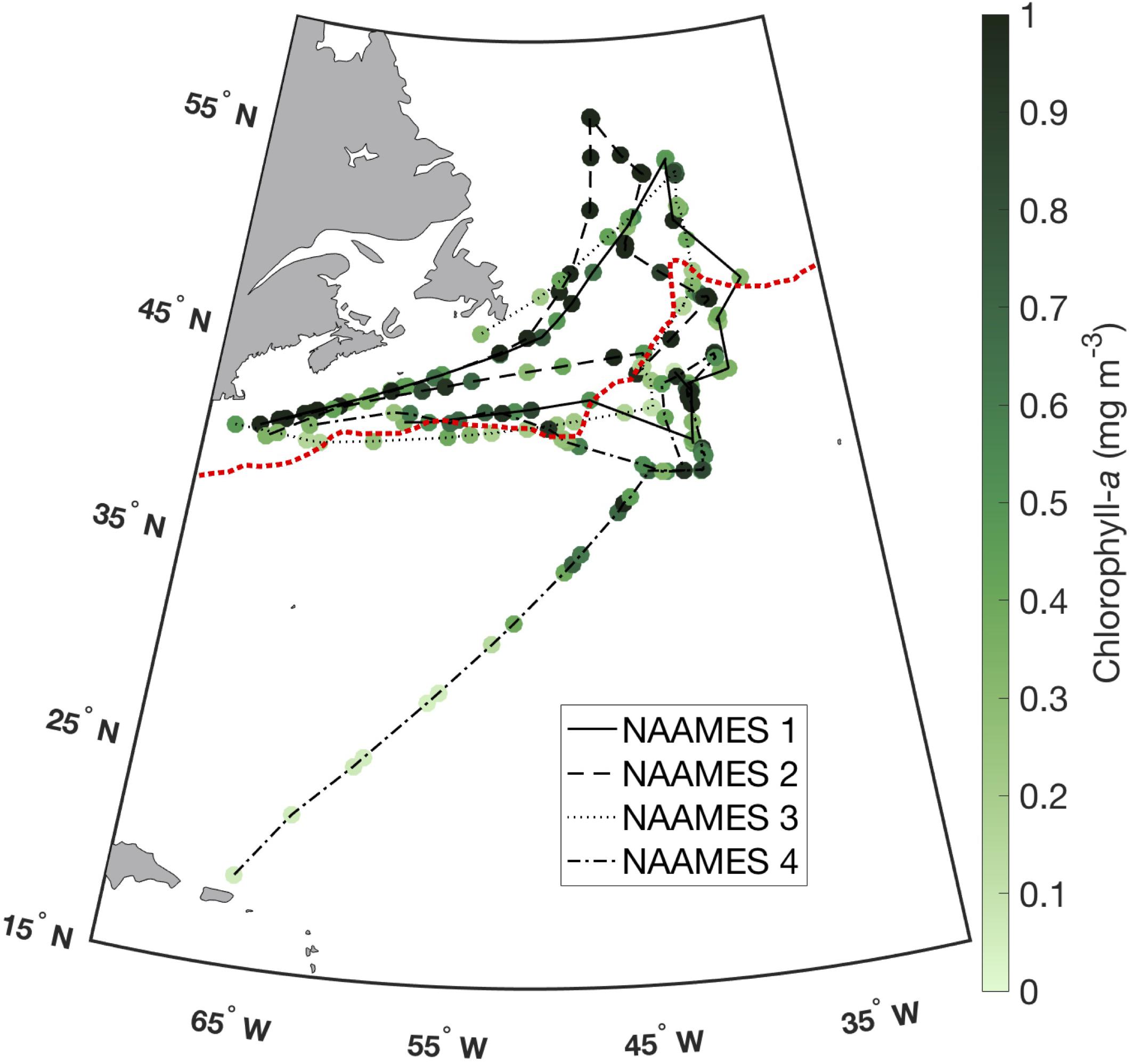
Figure 1. Surface ocean total chlorophyll-a concentration from HPLC (N = 229) on NAAMES 1 (solid line), NAAMES 2 (dashed line), NAAMES 3 (dotted line), and NAAMES 4 (dash-dot line). Subpolar (north of dashed red line) and subtropical (south of dashed red line) provinces are delineated as defined by Della Penna and Gaube (2019).

FIGURE 2

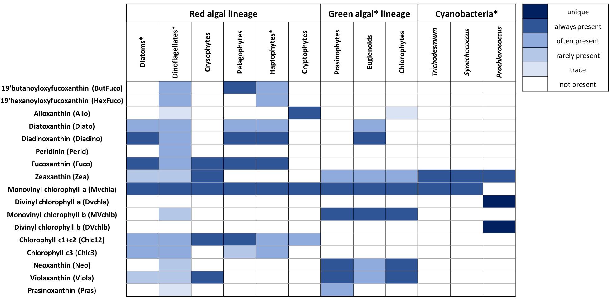
Figure 2. Summary of 17 pigments used in this analysis (16 accessory pigments and monovinyl chlorophyll-a) and the distribution of these pigments across twelve taxonomic groups, including the five major taxonomic groups identified in this analysis (starred). Known distributions of each pigment in each group (for the species in each group that have been cultured and had HPLC analysis performed) are shown (adapted from Jeffrey et al., 2011 and references therein).

The remaining sixteen pigments used in this analysis (and their abbreviations) are: 19’-hexanoyloxyfucoxanthin (HexFuco), 19’-butanoyloxyfucoxanthin (ButFuco), alloxanthin (Allo), fucoxanthin (Fuco), peridinin (Perid), diatoxanthin (Diato), diadinoxanthin (Diadino), zeaxanthin (Zea), divinyl chlorophyll a (DVchla), monovinyl chlorophyll b (MVchlb), divinyl chlorophyll b (DVchlb), chlorophyll c₁ + c₂ (Chlc12), chlorophyll c₃ (Chlc3), neoxanthin (Neo), violaxanthin (Viola), and prasinoxanthin (Pras). The chemotaxonomic utility of the pigments used in data-driven community analyses is illustrated in Figure 2, adapted from Jeffrey et al. (2011) and references therein, which denotes many common combinations of pigments found in different taxonomic groups of phytoplankton relevant to the North Atlantic Ocean. Prior to any of the following statistical analyses, all pigments were normalized to total chlorophyll-a concentration, given the high degree of co-linearity between absolute pigment concentrations (Supplementary Figure S1).

The HPLC pigment data are also compared to matched samples of inorganic nutrient concentration, underway temperature and salinity, and particle backscattering at 532 nm (as a proxy for particle concentration). All pigment, flow cytometry, and environmental data and descriptions of their collection and analyses are available on NASA’s SeaBASS data repository¹. Flow cytometry data are discussed in more detail below.

Flow Cytometry Dataset Summary

Flow cytometry analyses were performed on whole unpreserved surface seawater samples collected directly from in-line near-surface sampling system and CTD mounted Niskin bottles into sterile 5 ml polypropylene tubes (3x rinsed) and immediately stored at ∼4°C until analysis on a BD Influx Cell Sorter (ICS). All samples were analyzed within 30 min or less from the time of collection. A minimum of ∼7,000 total cells were interrogated per sample and counts were transformed into concentrations using calculated sample flow rates (Graff and Behrenfeld, 2018). The ICS was calibrated daily with fluorescent beads following standard protocols (Spherotech, SPHERO^TM 3.0 μm Ultra Rainbow Calibration Particles).

Flow cytometry data were broadly classified into cyanobacteria and eukaryotic phytoplankton with distinction being made between Prochlorococcus and Synechococcus for the cyanobacteria and pico- and nanoeukaryotes being defined based upon groupings of scattering and fluorescence properties that are associated with these groups. The BD ICS used during NAAMES was equipped with a 100 μm nozzle which has an upper cell size limit for analysis of ∼55–64 μm as determined in the lab and at sea using cultures. As with all particle counting methods, constraints of the volume of water that can be realistically analyzed also limit the number of observations made for the largest cells within each sample. For all analyses presented here, the concentration of cells in each class (Prochlorococcus, Synechococcus, picoeukaryotes, and nanoeukaryotes) was normalized to the total concentration of cells measured by flow cytometry.

Hierarchical Cluster Analysis

A hierarchical cluster analysis was performed on the NAAMES 1-4 HPLC pigment dataset, using all sixteen pigments described above after normalization to Tchla (e.g., Fuco:Tchla, etc.). This method uses Ward’s linkage method (the inner squared distance), based on the correlation distance (1-R, where R is Pearson’s correlation coefficient between phytoplankton pigment ratios), as in Latasa and Bidigare (1998) and Catlett and Siegel (2018). A linkage cutoff distance of 1 is used to divide the resulting dendrogram into distinct phytoplankton community clusters. The correlation distances between samples were then used to assign each sample to one of the resulting clusters.

Empirical Orthogonal Function (EOF) Analysis

An Empirical Orthogonal Function (EOF) analysis was performed on the NAAMES 1-4 surface HPLC pigment dataset to evaluate the co-variability in groups of phytoplankton pigments (following Catlett and Siegel, 2018; Kramer and Siegel, 2019). This analysis decomposes the data into dominant orthogonal functions descriptive of the major modes of variability in the dataset. The percent variance explained by each mode decreases with higher modes, i.e., Mode 1 describes the most variance in the dataset, thus only the lowest few modes are useful for interpreting a dataset. For each mode, an EOF analysis results in both the loadings over the entire dataset and amplitude functions for each sample. The loadings describe the correlation between the mode of variability and the input variables (in this case, ratios of phytoplankton pigments to Tchla) while the amplitude functions describe the strength of each mode at each sample location. The summed product of the loadings and amplitude functions over all of the EOF modes enables reconstruction of the original dataset. Pigment concentrations (normalized to Tchla) were mean-centered and normalized by their standard deviation before EOF analysis. Correlations between the dominant EOF modes and several relevant environmental variables (specifically latitude, temperature, salinity, and inorganic nutrient concentrations) were also considered.

Network-Based Community Detection Analysis

To perform the network-based community detection analysis, the NAAMES 1-4 HPLC pigment dataset was first transformed into a symmetrical adjacency matrix. The adjacency matrix describes the strength of the correlation between two nodes (here, between sampling sites) for all 229 sampling sites; these correlations describe the edges connecting the nodes. Pearson’s correlation coefficients were used to describe the relationships between nodes based on the ratios of each pigment normalized to Tchla. The edges between nodes were weighted following the Weighted Gene Co-Expression Network Analysis (WGCNA; Zhang and Horvath, 2005):

$$a_{ij}={\left|corr(x_i,x_j)\right|}^{\mathrm{\beta }}(1)$$

where a_ij is the adjacency matrix, corr(x_i,x_j) is the Pearson correlation coefficient between nodes (sampling sites) x_i and x_j, and β is a scaling term determined based on the average correlation coefficient in the input matrix (here β = 6, as in Zhang and Horvath, 2005). The WGCNA was chosen because it was developed for networks similar to the one used here, which has many nodes (229), each of which encompasses multiple traits (ratios of sixteen pigments to Tchla).

Next, community detection analysis was performed on the adjacency matrix using the modularity_und.m function, which is part of the Brain Connectivity Toolbox² developed for MATLAB as detailed in Rubinov and Sporns (2010). This method determines the number and type of communities that maximize the modularity of the network. Modularity refers to the connectedness of the network within communities: modularity of 0.3 or above is considered high and indicates highly interconnected sites within each community with weaker between-group connections. The output of this function gives a community assignment to each sampling site in the matrix based on the relatedness of the sixteen pigment ratios. The mean ratios of biomarker pigments in each community were used to determine the taxonomic significance of the community.

Results

The NAAMES 1-4 surface HPLC pigment dataset represents a wide range of environmental and ecological conditions (Table 1). NAAMES 2 (May–June) featured the coldest mean surface water temperature, highest mean surface Tchla concentration, and highest mean surface concentrations of nitrate. The highest mean Fuco:Tchla and mean Perid:Tchla ratios were also found in the surface ocean on NAAMES 2, suggesting more diatoms and dinoflagellates compared with other cruises. On NAAMES 3 (August-September), the mean surface ocean water temperature was the warmest of the four cruises, and the mean concentrations of Tchla and nitrate were the lowest. During this cruise, the mean ratios of HexFuco:Tchla and Zea:Tchla were the highest, indicating more haptophytes and picophytoplankton (including cyanobacteria). NAAMES 1 (November) and NAAMES 4 (March-April) had mid-range mean surface water temperature and nutrient concentrations. The highest mean ratio of MVchlb:Tchla, which is a biomarker pigment for all green algae, was found on NAAMES 1, while the lowest mean ratios of MVchlb:Tchla and Perid:Tchla (dinoflagellates) were found on NAAMES 4.

TABLE 1

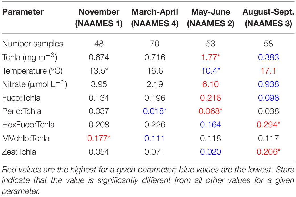
Table 1. Summary of environmental and ecological variables for surface samples on NAAMES 1-4.

Hierarchical Cluster Analysis

Five distinct phytoplankton pigment clusters emerge from the hierarchical cluster analysis of pigment ratios normalized to Tchla across the four NAAMES cruises (Figure 3A). The associations between pigment ratios can be used to infer the taxonomic designation of each major cluster (Figure 2). Cyanobacterial pigments (Zea, DVchla, DVchlb) are strongly correlated to each other and separate from all other pigments. Diatom pigments (Fuco, Chlc12) and dinoflagellate pigments (Perid) also separate from all other pigments, and from each other. Haptophyte pigments (HexFuco, ButFuco, Chlc3) and green algal pigments (MVchlb, Neo, Pras, Viola) are broadly linked but separate from each other and separate from the clusters of either cyanobacteria or diatoms and dinoflagellates. Allo (a cryptophyte biomarker) is correlated with green algal pigments, although cryptophytes are red algae (Figure 2). Thus, the hierarchical cluster analysis identified five distinct clusters of community types: diatom, dinoflagellate, green algae, haptophyte, and cyanobacteria.

FIGURE 3

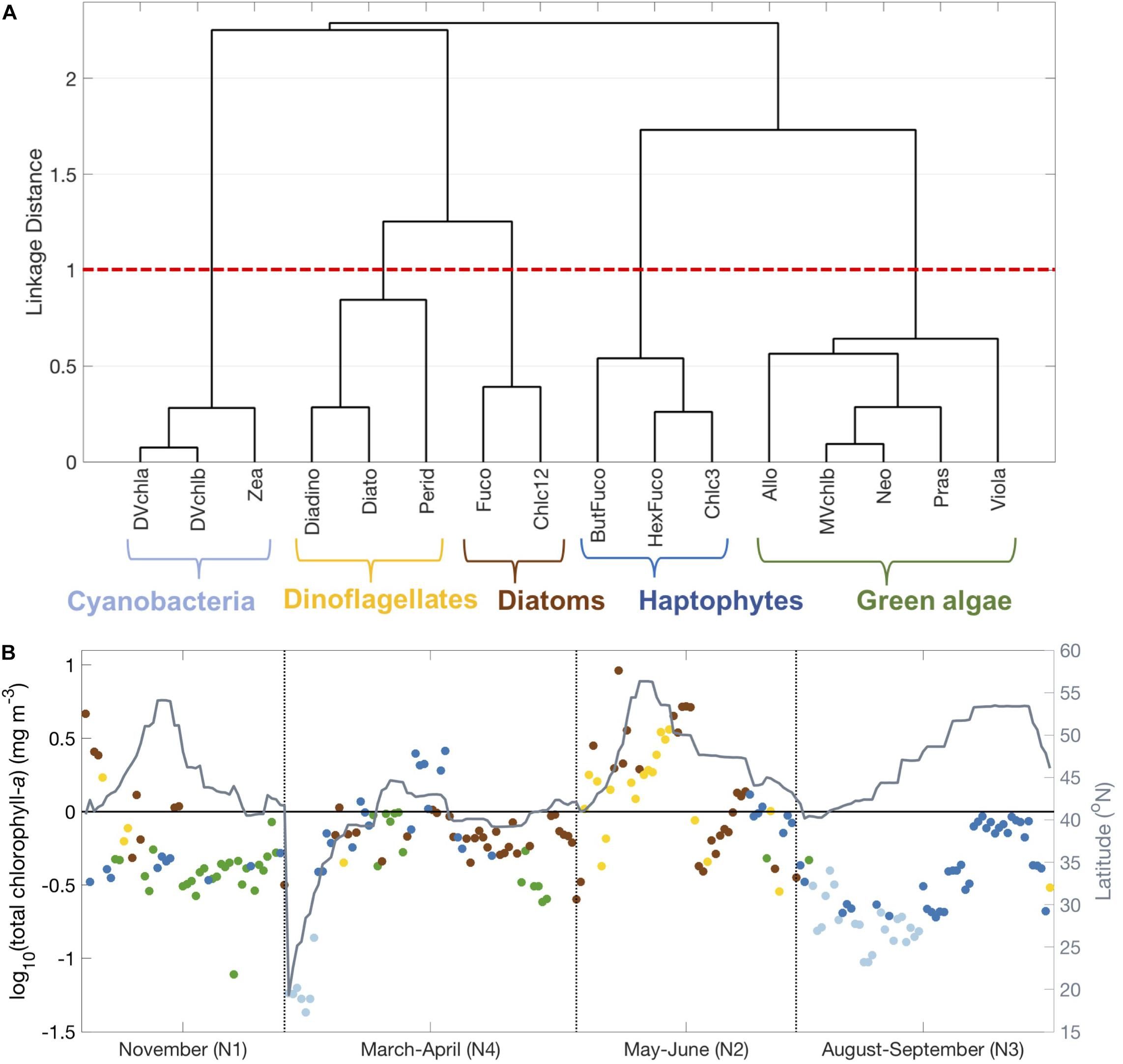
Figure 3. Hierarchical clustering of phytoplankton pigment ratios to total chlorophyll-a concentration. (A) Dendrogram showing five major phytoplankton pigment groups delineated with brackets, defined by a linkage distance cutoff of 1 (dashed red line). (B) Spatiotemporal distribution of surface samples on NAAMES colored by the cluster to which that sample was assigned (light blue = cyanobacteria, dark blue = haptophytes, green = green algae/mixed, brown = diatoms, gold = dinoflagellates).

The spatiotemporal distribution of these five clusters shows clear seasonal and latitudinal patterns (Figure 3B and Supplementary Figure S2). In the early spring (NAAMES 4) and at high latitudes (NAAMES 2), most samples are in the diatom and dinoflagellate clusters. In the late summer (NAAMES 3) and at low latitudes (beginning of NAAMES 4), nearly all samples are in the cyanobacteria cluster. In the early winter (NAAMES 1) and during transitions between the shelf to the open ocean (NAAMES 2-4), more samples in the green algae cluster were observed. Finally, samples in the haptophyte cluster were observed at mid-latitude from late summer (NAAMES 3) into the early winter (NAAMES 1) and again in the early spring (NAAMES 4).

EOFs

While hierarchical cluster analysis divides the pigments and samples into distinct groups, Empirical Orthogonal Function analysis provides spatiotemporal resolution for covariation in pigment variability. EOFs are represented by loadings that show the relative contribution of each pigment ratio, as well as amplitude functions (AFs) that show the spatial distribution of the intensity of each EOF mode at each sampling site (Figure 4 and Supplementary Figure S3). Here, the first four modes of the EOF analysis were used to show major modes of variability in pigment composition and concentration on NAAMES 1-4, including the correlation coefficients between each pigment used in this analysis and the first four EOF modes (Supplementary Table S1). The first four EOF modes explain 77.7% of the variability in the dataset.

FIGURE 4

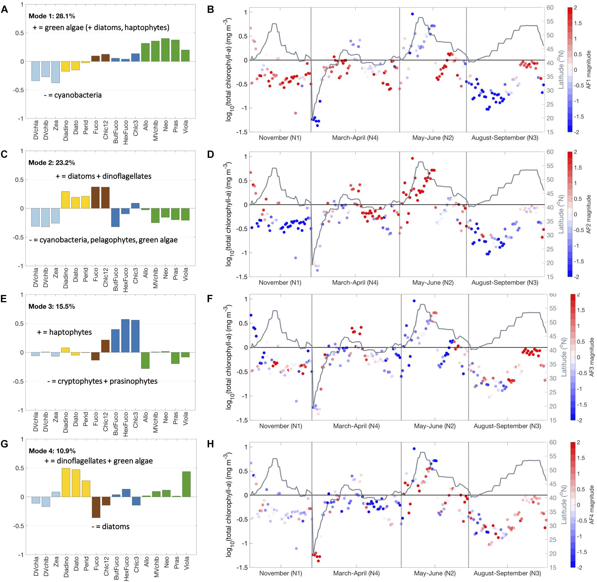
Figure 4. Empirical orthogonal functions for Mode 1 (A,B), 2 (C,D), 3 (E,F), and 4 (G,H), calculated for phytoplankton pigment ratios to total chlorophyll-a concentration. Loadings are colored based on pigment clusters (Figure 3): light blue (cyanobacteria), dark blue (haptophytes), green (green algae), brown (diatoms), and gold (dinoflagellates). Amplitude function magnitude is indicated as positive (red) or negative (blue) for each sample and latitude is in gray.

Mode 1 explains 28.1% of the overall variability and separates green algae (positive) from cyanobacteria (negative) (Figure 4A). Mode 1 is most negative at low latitudes (NAAMES 4 transit) and in the late summer (NAAMES 3) and most positive in the early winter (NAAMES 1) (Figure 4B). Mode 2 explains 23.2% of the all variability and separates diatoms and dinoflagellates (positive) from cyanobacteria, pelagophytes, and green algae (negative) (Figure 4C). Mode 2 is most positive at high latitude and in late spring (NAAMES 2). This mode is most negative at low latitude (NAAMES 4 transit), in late summer (NAAMES 3), and in early winter (NAAMES 1) (Figure 4D). Mode 3 explains 15.5% of the variability in the dataset and separates haptophytes from all other phytoplankton (positive), notably cryptophytes and prasinophytes (negative) (Figure 4E). This mode is most positive in late summer (NAAMES 3) and in transitions between major water masses (NAAMES 4 transit) (Figure 4F). Mode 4 explains 10.9% of the total variability; this mode is the first to separate diatoms (negative) from dinoflagellates (positive) (Figure 4G). Mode 4 is most positive in summer (NAAMES 2 and 3) and most negative in early spring and late summer (NAAMES 4 and 3) (Figure 4H). Thus, the EOF analysis identifies the same five phytoplankton pigment communities as the hierarchical cluster analysis, as well as more and different communities that emerge at higher modes of variability.

Network-Based Community Detection

The network-based community detection method employed here identifies four major phytoplankton pigment communities (Figure 5 and Supplementary Figure S4). In identifying these communities, this method aims to maximize the modularity of the network. Modularity is used as a metric for the connectedness between communities vs. within communities. Values of modularity >0.3 are considered high (Newman, 2006). The modularity for the NAAMES surface HPLC pigment ratio network was 0.33, suggesting high similarity between samples identified to be within the same community and robust separation of community types using this method. The taxonomic designation of each major phytoplankton pigment community was determined by the mean pigment to Tchla ratio of five biomarker pigments for each community (Figure 6). The first community has the highest mean ratios of Fuco and Perid to Tchla, suggesting high concentrations of diatoms and dinoflagellates (Figures 6A,B). The second community has the highest mean ratio of HexFuco to Tchla, indicating a haptophyte community (Figure 6C). The third community has the highest ratio of MVchlb:Tchla, which is found in green algae (Figure 6D). Finally, the fourth community has the highest ratio of Zea:Tchla, suggesting high concentrations of picoplankton and cyanobacteria (Figure 6E).

FIGURE 5

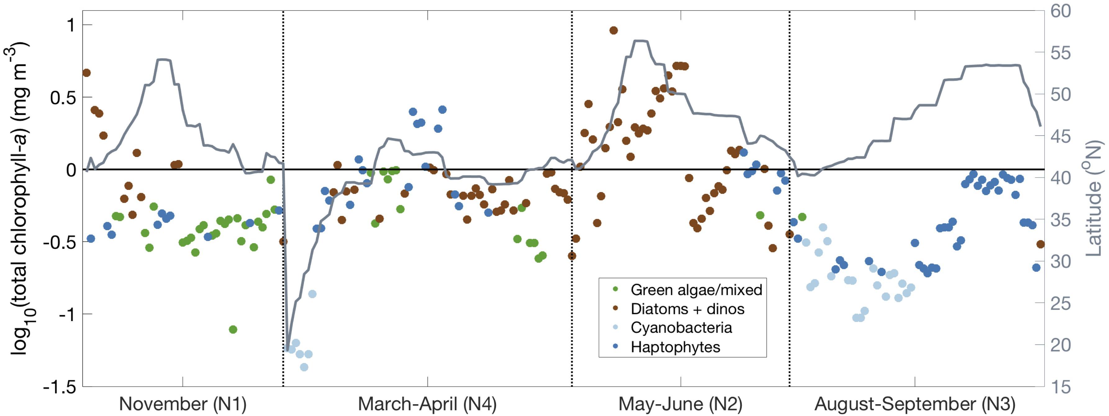
Figure 5. Results of network-based community detection (undirected modularity) for all surface samples. Samples are colored based on the dominant community determined from the community detection analysis: light blue (cyanobacteria), dark blue (haptophytes), green (green algae), brown (diatoms and dinoflagellates). Latitude plotted in gray.

FIGURE 6

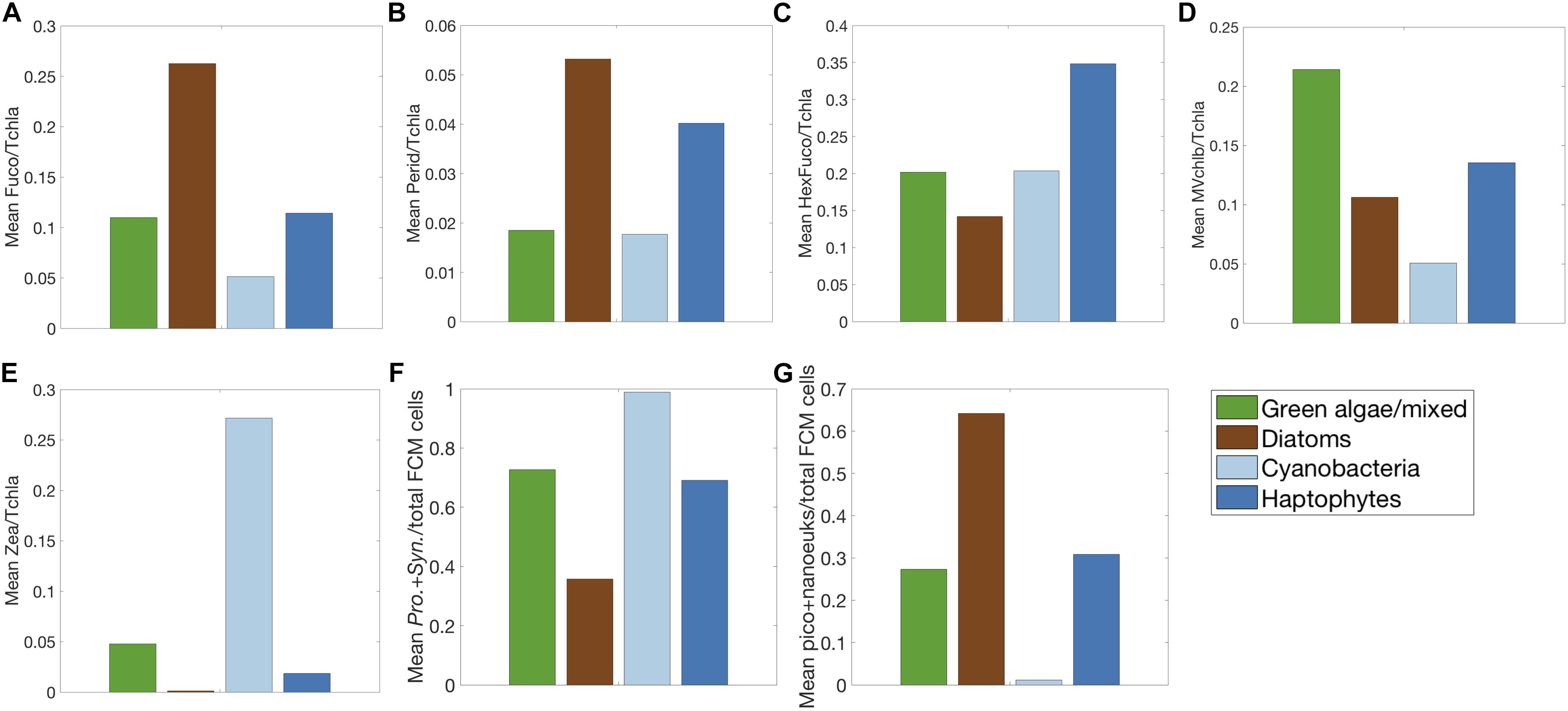
Figure 6. Mean pigment ratios to total chlorophyll-a for five biomarker pigments: (A) fucoxanthin, (B) peridinin, (C) 19’hexanoyloxyfucoxanthin, (D) mono-vinyl chlorophyll b, (E) zeaxanthin and (F) Prochlorococcus + Synechococcus, and (G) pico- and nanoeukaryote fractions of total cells measured by FCM for each community detected in the community detection analysis (light blue = cyanobacteria, dark blue = haptophytes, green = green algae/mixed, brown = diatoms and dinoflagellates).

These four communities are unequally distributed across NAAMES 1-4 (Figure 5). NAAMES 1 features the most samples in the green algal community. NAAMES 2 features primarily samples assigned to the diatom and dinoflagellate community, particularly at high latitude. On NAAMES 3, most samples at lower latitudes are assigned to the cyanobacteria community, while higher latitude samples are generally assigned to the haptophyte community. Finally, the transit through the Sargasso Sea on NAAMES 4 shows a transition from cyanobacteria to haptophytes to diatoms and dinoflagellates with increasing latitude and inorganic nutrient concentration and decreasing water temperature. The absence of certain communities on each cruise is also notable: while all four communities were present on NAAMES 4, there were no samples in the cyanobacteria community on NAAMES 1 or NAAMES 2, and only two samples in the diatom and dinoflagellate communities on NAAMES 3. There was only one sample in the green algal community for each cruise on NAAMES 2 and 3.

Combining Network-Based Community Detection and EOF Analyses

While diatoms and dinoflagellates were separated in the hierarchical cluster and EOF analyses presented here, these groups were combined in the network-based community detection analysis, prompting further examination of these results. The results of the EOF analysis were combined with the communities identified by the network-based community detection analysis in order to separate dinoflagellates from diatoms (Figure 7 and Supplementary Figure S5). The Mode 2 AF is positively correlated with both diatom and dinoflagellate pigments (Figure 4C) while the Mode 4 AF separates diatom (negative) and dinoflagellate (positive) pigments (Figure 4G). When these AFs are regressed against each other (Figure 7A), a distinct subset of samples in the diatom community (positive Mode 2 and negative Mode 4) separates from samples in the dinoflagellate community (positive Modes 2 and 4). The samples in the diatom community are enclosed with an ellipse designed to include all samples within ± 2 standard deviations of the mean AF value for each EOF mode. The samples in the dinoflagellate community (samples in the diatom community with positive AF values for Modes 2 and 4) become a fifth taxonomic community that can be isolated from the four communities already identified. The ratios of each biomarker pigment to Tchla for these five communities further validate the existence of a dinoflagellate pigment community (Supplementary Figure S2).

FIGURE 7

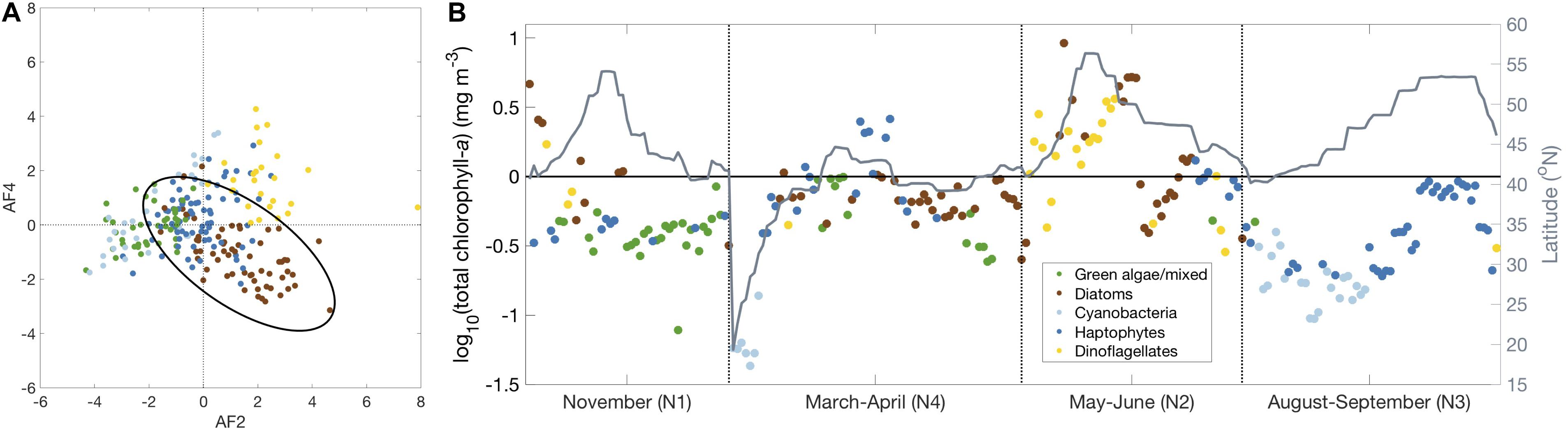
Figure 7. (A) Amplitude function of Mode 4 vs. Mode 2. When Mode 2 and Mode 4 are both positive, dinoflagellates can be separated from diatoms. Using this metric, samples are colored by the dominant community detected in the community detection analysis (light blue = cyanobacteria, dark blue = haptophytes, green = green algae/mixed, brown = diatoms, gold = dinoflagellates). The black ellipse encircles 95% of the diatom samples. (B) Resulting spatiotemporal distribution of all five communities identified using network-based community detection and EOF regression (latitude plotted in gray).

The spatiotemporal distribution of the samples in the dinoflagellate community (Figure 7B) shows that the dinoflagellate community is most common on NAAMES 2, particularly at the highest latitudes, but also on the cruise track from the shelf to the open ocean. There are also samples in the dinoflagellate community found on the shelf on NAAMES 1 and 3. Clearly, the five taxonomic groups identified from EOF and network-based community detection analyses have different spatiotemporal distributions and represent different ecological and environmental conditions sampled on NAAMES. The five communities can be further divided based on the mean values for environmental and chemotaxonomic parameters (Table 2). The cyanobacteria community has the lowest mean surface Tchla concentration, nutrient concentrations, and ratios of Fuco and MVchlb to Tchla. This community also has the highest mean surface water temperature and Zea to Tchla concentrations. Alternately, the dinoflagellate community has the lowest mean surface water temperature and the highest mean surface Tchla concentration, nutrient concentrations, and Perid:Tchla ratio. As expected, the diatom community has the highest mean Fuco:Tchla ratio, the green algae community has the highest mean MVchlb:Tchla ratio, and the haptophyte community has the highest mean HexFuco:Tchla ratio. It is notable that there is also a significantly high ratio of Fuco:Tchla found in the dinoflagellate community, which is unsurprising as many species in this group contain Fuco (Figure 2).

TABLE 2

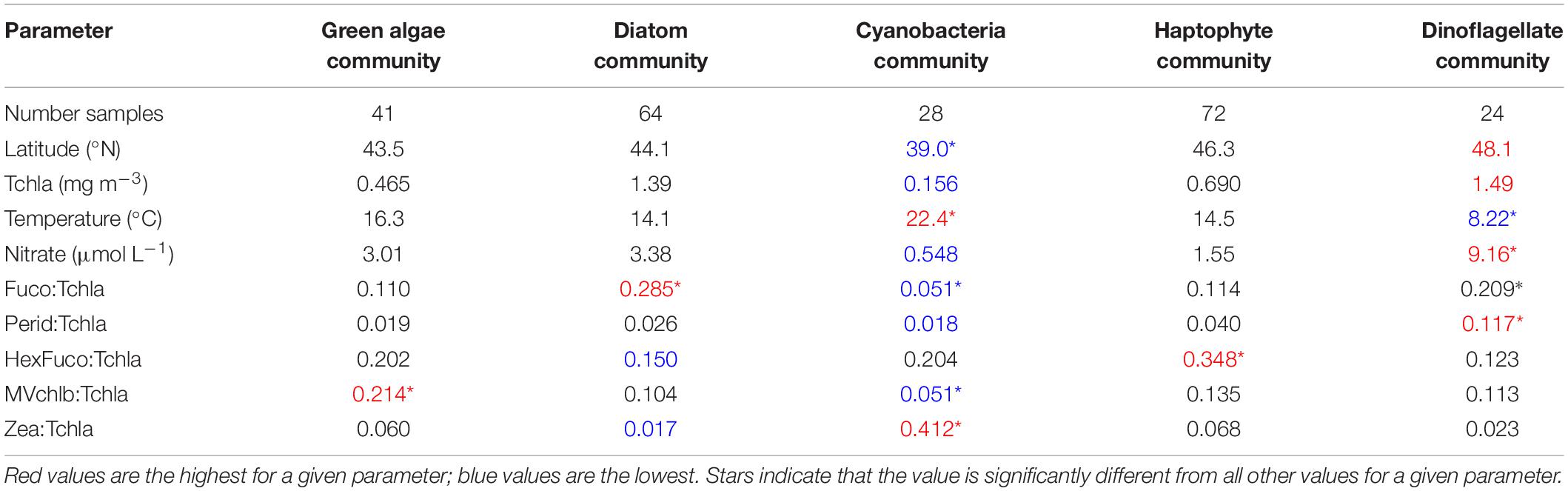
Table 2. Summary of environmental and ecological variables for surface samples on NAAMES 1-4, divided into results of network-based community detection analysis.

When the distribution of these five communities is compared proportionally for each NAAMES cruise, a seasonal cycle of phytoplankton community composition emerges (Figure 8). In early winter (NAAMES 1), over 50% of the surface samples were assigned to the green algal community, with additional contributions from the haptophyte and diatom communities of ∼20% each. By early spring (NAAMES 4), the diatom community were nearly 50% of the total number of samples, with contributions by green algae and haptophytes of ∼20% each. Samples in the cyanobacteria community also appeared, from the NAAMES 4 transit through the Sargasso Sea (Figure 7B). Diatoms continued to comprise a large proportion of the samples in early summer (NAAMES 2). The dinoflagellate community also comprised more than 1/3 of the total samples at this time of year, while ∼20% of the samples were in the haptophyte community. Finally, in late summer (NAAMES 3), samples in the haptophyte community comprised over 60% of the overall samples, with the cyanobacteria community comprising the majority of the rest of the samples. NAAMES 3 featured one sample in the green algal community and one in the dinoflagellate community, both on the shelf and not in the open ocean.

FIGURE 8

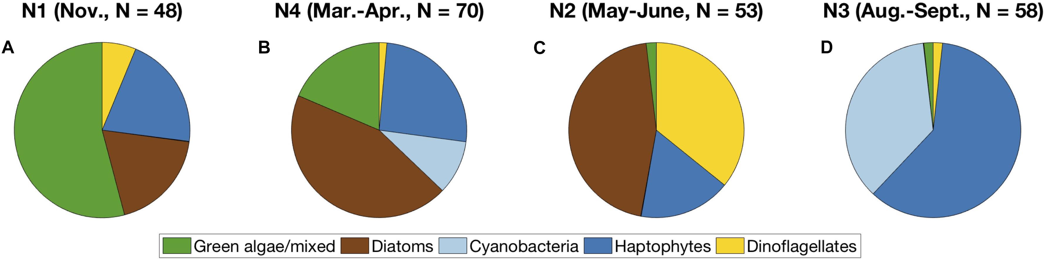
Figure 8. Proportion of samples in each community detected using network-based community detection and EOF regression on NAAMES 1-4, arranged in seasonal order: (A) winter, (B) early spring, (C) early summer, (D) early fall. Colors correspond to the dominant community (light blue = cyanobacteria, dark blue = haptophytes, green = green algae, brown = diatoms, gold = dinoflagellates).

The results of the merged EOF and network-based community detection analyses compare favorably to the communities determined by the hierarchical cluster analysis (Figures 3B, 7B). The spatiotemporal distribution of the samples identified in each community by the two methods is nearly identical. The number of samples in each community is also quite similar, although the merged EOF-network method identified more diatoms and fewer dinoflagellates compared to the hierarchical cluster analysis (Supplementary Table S2).

HPLC Pigments and Flow Cytometry

The results presented here from HPLC pigments provide a relatively lower taxonomic resolution in comparison to other methods: a maximum of five phytoplankton communities can be detected in the surface ocean on NAAMES using pigment-based taxonomy. Fortunately, 161 of the 229 samples used in the original HPLC pigment analysis also had concurrent FCM samples taken for characterization and quantification of four distinct phytoplankton groups. The same statistical analyses were applied to this matched HPLC-FCM dataset (Figure 9 and Supplementary Figure S7). In the hierarchical cluster analysis (Figure 9), relative Prochlorococcus cell abundances cluster with DVchla, DVchlb, and Zea. Prochlorococcus spp. uniquely contain DVchla and DVchlb, while Zea is an accessory pigment in Prochlorococcus and other cyanobacteria. Relative Synechococcus cell abundances form their own cluster separate from all other taxonomic groups. Finally, relative pico- and nanoeukaryote cell abundances cluster with diatom pigments, though diatoms are typically considered nano- to micro-sized phytoplankton.

FIGURE 9

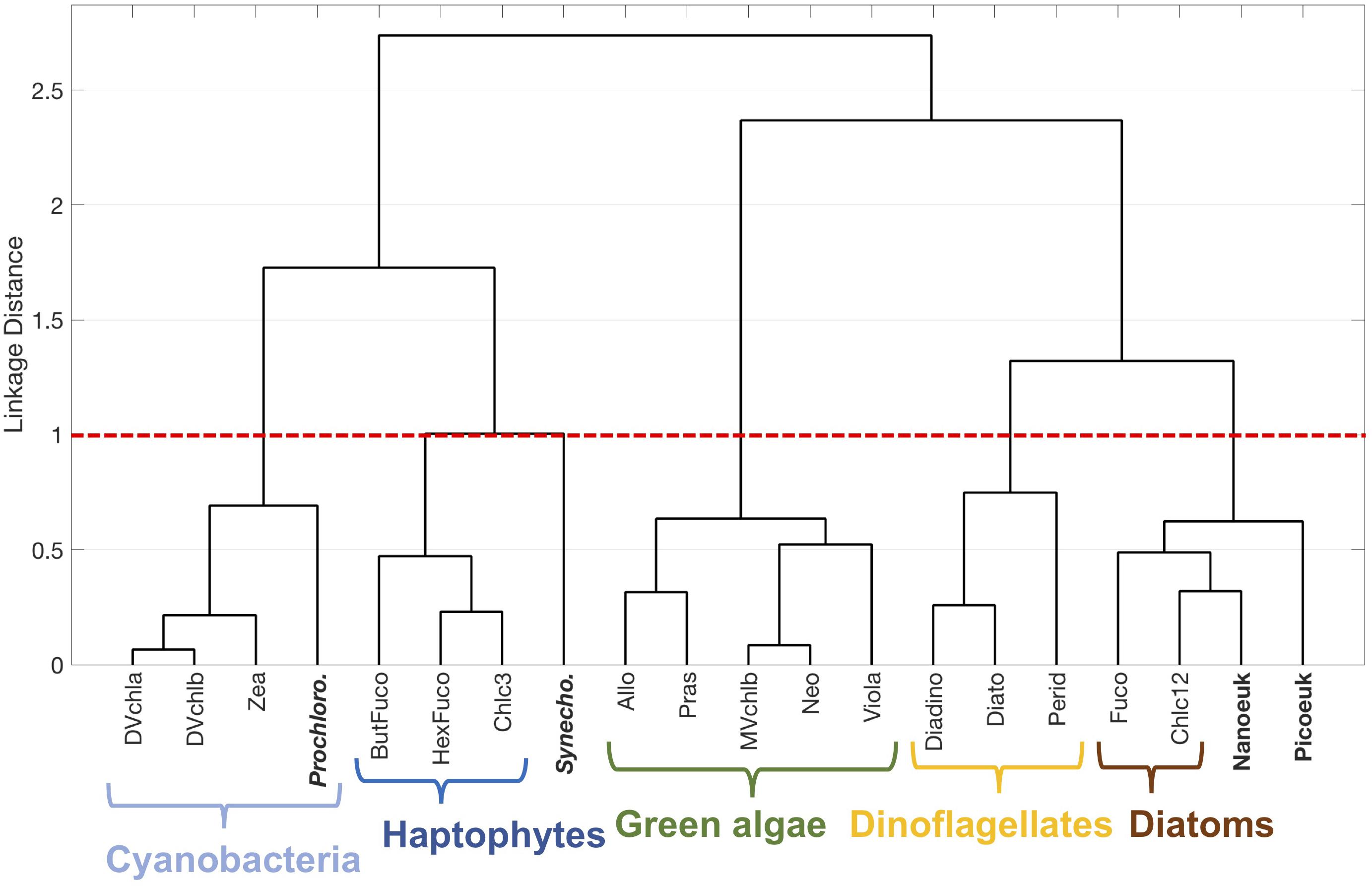
Figure 9. Hierarchical clustering of phytoplankton pigment ratios to total chlorophyll-a concentration and flow cytometry group cell counts to total cell counts. Five major phytoplankton pigment groups (cyanobacteria, haptophytes, green algae, diatoms, and dinoflagellates) are delineated with brackets.

The EOF loadings show similar patterns: the five major taxonomic communities identified by HPLC pigments separate from one another, Prochlorococcus relative cell abundances covary with cyanobacterial pigments, pico- and nanoeukaryote cell abundances covary with diatom and dinoflagellate pigments, and Synechococcus relative cell abundances separate from all other taxonomic groups in Mode 1 (Supplementary Figure S7A). However, the EOF loadings add nuance to the results of the hierarchical cluster analysis. For instance, Synechococcus relative cell abundances also covary with green algal pigments, while picoeukaryote relative cell abundances covary with green algal and cyanobacterial pigments (Modes 2 and 3, Supplementary Figures S7B,C). Finally, nanoeukaryote relative cell abundances covary most strongly with diatom and dinoflagellate pigments (Modes 1 and 2, Supplementary Figures S7A,B).

The patterns observed in the hierarchical cluster analysis are further reinforced when comparing the relative fractions of cyanobacteria cells and eukaryotic cells as measured by flow cytometry in each pigment community identified in the network-based community detection analysis (Figure 5 and Supplementary Figure S6). Unsurprisingly, the highest fractions of Prochlorococcus and Synechococcus were found in samples assigned to the cyanobacterial community (Figure 5F and Supplementary Figure S6F). Similarly, echoing the results of the hierarchical cluster and EOF analyses, the highest fractions pico- and nanoeukaryotic cells were found in the diatom (Figure 5G and Supplementary Figure S6G) and dinoflagellate (Supplementary Figure S6G) communities. While diatoms and dinoflagellates are traditionally designated to the microphytoplanton size fraction in pigment-based methods, there are many nano-sized members of both of these groups (e.g., Leblanc et al., 2018).

Discussion

Seasonal Succession of Phytoplankton in the North Atlantic

A major goal of the NAAMES field campaign was to characterize the phytoplankton dynamics over the seasonal cycle in the subarctic Atlantic Ocean (Behrenfeld et al., 2019). This analysis describes the surface ocean phytoplankton community at coarse taxonomic resolution, but with coverage of all four cruises and seasons. Despite the high dynamic ranges in Tchla, surface ocean temperature, nutrient concentrations, and biomarker pigment ratios to Tchla across the four cruises, the results presented here show consistent retrieval across data-driven statistical analyses and identification of five taxonomically distinct communities of phytoplankton on the four NAAMES cruises. The five communities that emerge can be characterized by five biomarker pigments: diatoms (Fuco), dinoflagellates (Perid), haptophytes (HexFuco), green algae (MVchlb), and cyanobacteria (Zea). Comparable analyses have shown that a maximum of four phytoplankton communities can be retrieved from HPLC pigments on global scales, but this regional example identifies five communities in the western North Atlantic, with dinoflagellates separating from diatoms, which does not occur globally (Kramer and Siegel, 2019). There were enough sites sampled on the four NAAMES cruises with high concentrations of dinoflagellate pigments that these pigments separate from diatom and other red algal pigments in hierarchical cluster and EOF analyses (Figures 2, 3). The designation of each sample to a distinct community in the network-based community detection analysis further allows for consideration of the spatiotemporal distribution of these five communities (Figure 7B).

The classic seasonal cycle of phytoplankton species succession in the North Atlantic begins with a spring diatom bloom, followed by a late summer to fall peak in haptophytes and dinoflagellates, transitioning to a winter community dominated by smaller phytoplankton, such as green algae and cyanobacteria (i.e., Taylor et al., 1993). While each NAAMES cruise represents only a snapshot of each season, in many ways, the seasonal progression of phytoplankton communities sampled on NAAMES 1-4 reflects this paradigm (Figure 8). An abundance of samples in the diatom community were found on the spring (NAAMES 4) and early summer (NAAMES 2) cruises during the onset and accumulation of the spring phytoplankton bloom. On NAAMES 4, haptophytes and green algae were also present. By early summer, dinoflagellates also comprised a large fraction of the community with diatoms. The transition from late summer into early fall (NAAMES 3) was dominated by samples in the haptophyte community with some cyanobacteria in the bloom decline. By early winter (NAAMES 1), the community is comprised of mostly green algae dominated samples with some haptophytes and diatoms. While each NAAMES cruise only captures 2–3 weeks of the surface ocean phytoplankton community, and phytoplankton community dynamics can change on the order of hours to days over the course of a month or a season, the changes in latitude on each NAAMES cruise increase the range of bloom states and phytoplankton communities sampled in the western North Atlantic Ocean. In order to further interpret these snapshots of the seasonal cycle, it will be necessary to consider the HPLC pigment data in the context of more continuously collected data from the North Atlantic, including satellite remote sensing of ocean color and autonomous bio-optical profiling floats (e.g., Bisson et al., 2019).

It does not appear that the five phytoplankton communities that can be separated using HPLC pigments have individual niches in the physical environment, though some communities are particularly prevalent under certain environmental conditions. Spatial patterns in community composition (Figures 3B, 7B) reflect trends in environmental variables (Table 2) that also confirm expectations of phytoplankton succession from previous studies. As expected, most samples taken at high latitudes with colder water temperatures and higher nutrient concentrations are assigned to the diatom and dinoflagellate communities, while cyanobacteria communities are only found at lower latitudes. Haptophyte and green algae communities are found throughout the mid-range of latitudes sampled on NAAMES, representing a broader range of temperatures and nutrient environments. These patterns are further reinforced by direct comparisons between environmental variables (Figure 10). Unsurprisingly, samples in the cyanobacteria community are mostly found the warmest, saltiest water (Figure 10A) with the lowest chlorophyll-a concentrations (Figure 10B) and the lowest concentrations of phytoplankton and other particles (using particle backscattering as a proxy for particle concentration; Figure 10C). Dinoflagellates and some diatoms are found mostly in the coldest, fresher water (Figure 10A), with high chlorophyll-a concentration (Figure 10B) and high concentrations of phytoplankton and other particles (Figure 10C). All haptophytes and green algae, along with a large fraction of the diatoms, fill in the mid-ranges of these environmental parameters. Ultimately, the spatiotemporal distribution of phytoplankton communities derived from HPLC pigments on NAAMES is broadly consistent with expected environmental controls on phytoplankton community composition.

FIGURE 10

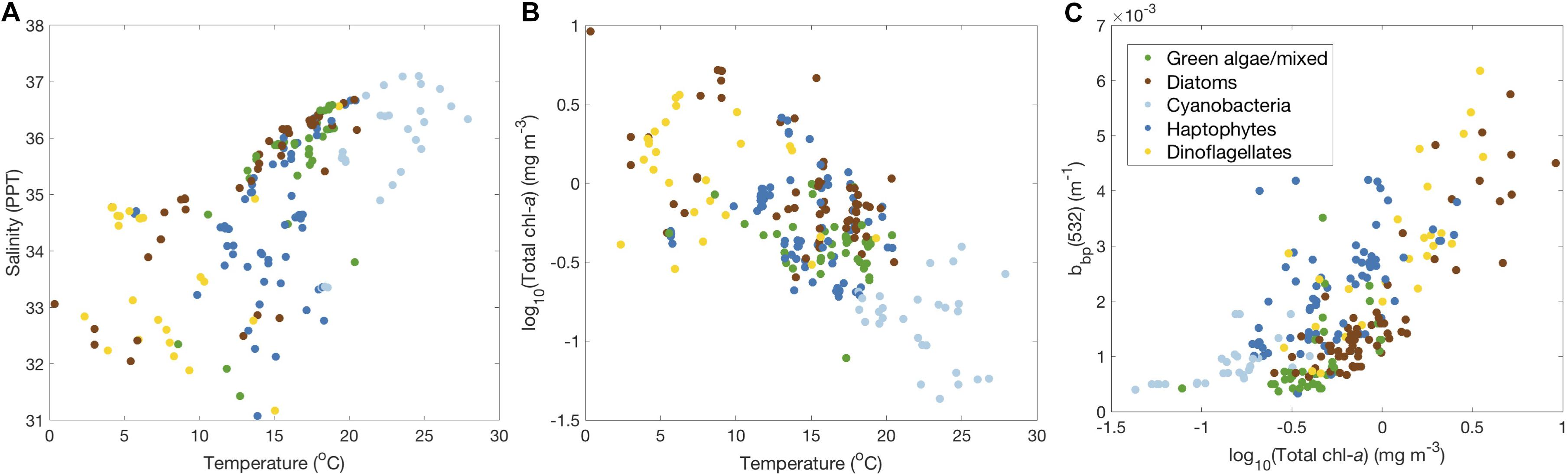
Figure 10. Regressions of physical and environmental parameters including (A) salinity vs. temperature, (B) total chlorophyll-a vs. temperature, and (C) particle backscattering (b_bp) at 532 nm vs. total chlorophyll-a, all colored by the dominant community (light blue = cyanobacteria, dark blue = haptophytes, green = green algae, brown = diatoms, gold = dinoflagellates).

Comparing Methods of Characterizing Phytoplankton Taxonomy on NAAMES

The taxonomic resolution provided by HPLC pigments in this study is too low to discern intricacies in these community dynamics, such as the dominant cell size in each community or the composition of species of the same major taxonomic group. Some pigment-based methods assume that biomarker pigments are confined to a given cell size distribution (i.e., Claustre, 1994; Uitz et al., 2006). For these methods, diatoms (Fuco) and dinoflagellates (Perid) are always considered microplankton (>20 μm), although there are important nano-sized members of both of these groups (2–20 μm; i.e., Leblanc et al., 2018). Quantitative imaging results from NAAMES suggest that pigment-based methods underestimate the contribution of nano-sized diatoms and dinoflagellates to cell counts, cell biovolume, and cellular carbon in this dataset (Chase et al., under review). DNA metabarcoding has also been applied to concurrent samples from NAAMES, and gives higher resolution taxonomic information, to species, group, or strain level, such as separation between high- and low-light variants of the cyanobacteria identified with HPLC pigments and flow cytometry (i.e., Bolaños et al., in review). While the taxonomic resolution of HPLC pigments is lower than the resolution provided by methods such as microscopy and imaging or DNA metabarcoding, these results still provide a low-level characterization of the surface ocean phytoplankton community in the western North Atlantic across a seasonal cycle. Other methods supplement the community assessment provided by HPLC to give a full picture of the phytoplankton community on NAAMES. A complete characterization of the phytoplankton ecosystem can then be used to investigate further components of the NAAMES field campaign, such as the role of community composition in net primary productivity and photoacclimation (i.e., Fox et al., 2020) or in biogenic aerosol production. While higher-resolution taxonomic data from other sources can add nuance and complexity to the results found from lower-resolution data, such as HPLC pigments, these different characterizations of taxonomy often complement each other. Each method presents an incomplete picture of phytoplankton taxonomy and cell size; thus, they must be combined for maximum information content. As a first step, flow cytometric characterization and quantification of the pico- and nano-sized cells confirms and supplements the results shown from pigment-based taxonomy (Figures 9 and Supplementary S7). The clustering of Prochlorococcus spp. with other cyanobacterial pigments is unsurprising, as Prochlorococcus uniquely contain divinyl chlorophylls rather than monovinyl chlorophyll-a, which all other phytoplankton taxa contain (Figure 2). Synechococcus spp., which contain MVchla and Zea, are most closely related to the haptophyte pigment community, suggesting co-occurrence of these communities in the environment given the weak but positive correlation between these communities (Supplementary Table S3). The relatively large linkage distance separating these communities means that Synechococcus is distinct from all other phytoplankton groups.

The clustering of pico- and nano-eukaryotes with pigments typically associated with diatom populations is unexpected, as diatoms are usually considered nano- to micro-sized phytoplankton. However, an EOF analysis including FCM data (Supplementary Figure S7) shows that relative picoeukaryote cell abundance is also correlated with pigments found in phytoplankton communities known to contain pico-sized members, such as green algae (Supplementary Figure S7A) and cyanobacteria (Supplementary Figure S7D). Relative nanoeukaryote cell abundance is also correlated with pigments found in dinoflagellates (Supplementary Figure S7B and Supplementary Table S3) and green algae (Supplementary Figure S7D). As the association of picoeukaryotes and diatoms is based on correlation, the EOF analysis adds necessary nuance to the relationship between relative picoeukaryote abundance and diatom pigments and better describes the composition of the nanoeukaryote community.

Ultimately, an analysis of taxonomy can only be as powerful as the quality of the input data. Other common pigment-based methods, such as CHEMTAX (Mackey et al., 1996), purport to separate more and different phytoplankton communities than were identified by the methods used here. CHEMTAX assumes linear independence of the pigments: the high degree of collinearity between HPLC pigments in this dataset makes it impossible to separate more distinct taxonomic groups than the five groups identified here (Supplementary Figure S1; Kramer and Siegel, 2019). CHEMTAX also assumes that the contributions of one or many pigments to individual phytoplankton groups are set and known. The NAAMES cruises surveyed a broad latitudinal range across four seasons under varying nutrient and light conditions, which likely led to varying pigment contributions across taxa and time (i.e., Schlüter et al., 2000; Havskum et al., 2004; Irigoien et al., 2004; Zapata et al., 2004). The data-driven statistical analyses performed here demonstrate how pigment-based methods are also limited by the conditions under which the data were collected. For instance, in the NAAMES dataset, the dinoflagellate community consistently separates from other communities, as dinoflagellates were often present during surface ocean sampling on NAAMES in high enough concentrations to comprise large fractions of both total cell counts and total chlorophyll concentration (Kramer and Siegel, 2019; Chase et al., 2020). Conversely, cryptophytes (a red alga, denoted by the biomarker pigment Allo) are never a large enough fraction of the community in this dataset to separate from the broader green algal community. As the assumptions made by CHEMTAX were not supported by this dataset, this method was not implemented here.

NAAMES in the Context of a Changing North Atlantic Ocean

The results presented here capture the surface ocean phytoplankton community of the western North Atlantic across four seasons, representing succession through different phases of phytoplankton bloom onset, accumulation, and decline. While the exact structuring of the phytoplankton community and ecosystem change on an interannual basis, these results can provide a baseline against which to consider future change. The North Atlantic phytoplankton bloom will undoubtedly change in a warming ocean (Boyd and Doney, 2002; Barton et al., 2016). The timing of bloom initiation, the extent and magnitude of the bloom, the structuring of the water column (impacting properties that influence bloom initiation and progression, such as mixed layer depth and nutrient concentration), the frequency and magnitude of other climate oscillations, etc., are all sensitive to changing surface and deep ocean temperatures (Henson et al., 2009; Racault et al., 2012; Behrenfeld, 2014). These events and parameters in turn have impacts on the resulting phytoplankton community composition and phenology. The diatom pigment community on NAAMES 1-4 was found predominantly in the spring to early summer, in water with cold temperatures and high nutrient concentrations (Table 2). Under future warming scenarios, a more highly stratified ocean would limit the injections of deep, nutrient-rich water to the surface ocean even during the spring bloom, and favor communities of smaller phytoplankton including dinoflagellates, haptophytes, and cyanobacteria (Falkowski and Oliver, 2007).

A changing ocean may also experience altered light availability, as the concentrations of phytoplankton and other absorbing ocean constituents [i.e., colored dissolved organic matter (CDOM), non-algal particles), as well as surface mixed layer depth, change with a warming climate (Dutkiewicz et al., 2019). The amount and the wavelength range of the remaining available light shapes the resulting phytoplankton community, both in the surface and at depth (Bidigare et al., 1990; Siegel et al., 1990; Huisman et al., 1999). Overlapping communities of phytoplankton with depth are often identified by changes in phytoplankton pigment composition and concentrations – but these same processes may occur throughout the euphotic zone, particularly if there is an increase in compounds that absorb in the same wavelength range as phytoplankton (such as elevated CDOM, which absorbs most strongly in the blue wavelengths, where Tchla and most phytoplankton accessory pigments also absorb light). Measurements of phytoplankton pigment composition in conjunction with phytoplankton absorption spectra can indicate that the communities have chromatically adapted to the shifting light field and optimized the narrowing niche of light and nutrients (Hickman et al., 2009). If the ratios of accessory pigments to Tchla change in the surface ocean under future warming scenarios, as phytoplankton adapt to changes in available light, historical data relating phytoplankton pigment ratios to taxonomy will not be able to describe the new relationships between pigments and taxonomy, and new relationships will have to be constructed.

Historically, the magnitude and extent of the North Atlantic bloom has been observed using satellite remote sensing (i.e., Siegel et al., 2002; Behrenfeld et al., 2013). Pigment-based methods are well suited to link satellite measurements to surface ocean ecology at coarse resolution given the impact of phytoplankton pigments on absorption, which directly alters the shape and magnitude of remote sensing reflectance. However, these methods are limited by both the spectral resolution of the satellite and the composition of the HPLC dataset used to calibrate and validate the satellite models (i.e., Kramer and Siegel, 2019; Werdell et al., 2019). Based on the results presented here, a future satellite model of phytoplankton community composition built for the western North Atlantic Ocean using this HPLC dataset for calibration and validation could retrieve at most 5 distinct phytoplankton communities. The addition of other data types, such as cell quantification with flow cytometry as shown here, can improve the confidence of these models to describe surface ocean phytoplankton ecology, particularly in a region of high variability and particular oceanographic and biogeochemical interest, such as the North Atlantic Ocean.

Data Availability Statement

The datasets generated for this study can be found in the NASA’s SeaBASS data repository: https://seabass.gsfc.nasa.gov/naames.

Author Contributions

SK led the analysis and writing of this manuscript. DS and JG provided comments, data, edits, and support.

Funding

SK was supported by a National Defense Science and Engineering Graduate Fellowship through the Office of Naval Research. Support for this work came from the National Aeronautics and Space Administration (NASA) to DS and JG as part of the North Atlantic Aerosols and Marine Ecosystems Study (NAAMES, grants NNX15AE72G and NNX15AAF30G) field campaign.

Conflict of Interest

The authors declare that the research was conducted in the absence of any commercial or financial relationships that could be construed as a potential conflict of interest.

Acknowledgments

We wish to thank Mike Behrenfeld for his work as Chief Scientist, the captains and crew of R/V Atlantis, and all scientists and technicians who helped with sample collection on NAAMES 1-4. Huge thanks are owed to Crystal Thomas at NASA GSFC for processing all HPLC samples from NAAMES with high precision and quick turnaround time. Thanks to Nils Haëntjens for help with compiling and organizing the FCM data. Thank you to Ali Chase and Luis Bolaños for helpful conversations and suggestions about this work in its early stages. The two reviewers provided comments that improved and strengthened this manuscript.

Supplementary Material

The Supplementary Material for this article can be found online at: https://www.frontiersin.org/articles/10.3389/fmars.2020.00215/full#supplementary-material

References

Anderson, C. R., Siegel, D. A., Brzezinski, M. A., and Guillocheau, N. (2008). Controls on temporal patterns in phytoplankton community structure in the santa barbara channel. California. J. Geophys. Res. 113, 1–16.

Google Scholar

Barlow, R. G., Mantoura, R. F. C., Gough, M. A., and Fileman, T. W. (1993). Pigment signatures of the phytoplankton composition in the northeastern Atlantic during the 1990 spring bloom. Deep Sea Res. II 40, 459–477. doi: 10.1016/0967-0645(93)90027-K

CrossRef Full Text | Google Scholar

Barnard, R., Batten, S., Beaugrand, G., Buckland, C., Conway, D. V. P., Edwards, M., et al. (2004). Continuous plankton records: plankton atlas of the North Atlantic Ocean (1958–1999). II. Biogeographical charts. Mar. Ecol. Prog. Ser. (Suppl) 11–75.

Google Scholar

Barton, A. D., Irwin, A. J., Finkel, Z. V., and Stock, C. A. (2016). Anthropogenic climate change drives shift and shuffle in North Atlantic phytoplankton communities. Proc. Natl. Acad. Sci. U.S.A. 113, 2964–2969. doi: 10.1073/pnas.1519080113

PubMed Abstract | CrossRef Full Text | Google Scholar

Behrenfeld, M. J. (2014). Climate-mediated dance of the plankton. Nat. Clim. Change 4, 880–887. doi: 10.1038/NCLIMATE2349

CrossRef Full Text | Google Scholar

Behrenfeld, M. J., Doney, S. C., Lima, I., Boss, E. S., and Siegel, D. A. (2013). Annual cycles of ecological disturbance and recovery underlying the subarctic Atlantic spring plankton bloom. Global Biogeochem. Cycles 27, 526–540. doi: 10.1002/gbc.20050

CrossRef Full Text | Google Scholar

Behrenfeld, M. J., Moore, R. H., Hostetler, C. A., Graff, J., Gaube, P., Russell, L. M., et al. (2019). The North Atlantic Aerosol and marine ecosystem study (NAAMES): science motive and mission overview. Front. Mar. Sci. 6:122. doi: 10.3389/fmars.2019.00122

CrossRef Full Text | Google Scholar

Bidigare, R. R., Marra, J., Dickey, T. D., Iturriaga, R., Baker, K. S., Smith, R. C., et al. (1990). Evidence for phytoplankton succession and chromatic adaptation in the Sargasso Sea during spring 1985. Mar. Ecol. Prog. Ser. 60, 113–122. doi: 10.3354/meps060113

CrossRef Full Text | Google Scholar

Bisson, K. M., Boss, E., Westberry, T. K., and Behrenfeld, M. J. (2019). Evaluating satellite estimates of particulate backscatter in the global open ocean using autonomous profiling floats. Opt. Expr. 27, 30191–30203. doi: 10.1364/OE.27.030191

PubMed Abstract | CrossRef Full Text | Google Scholar

Boyd, P. W., and Doney, S. C. (2002). Modelling regional responses by marine pelagic ecosystems to global climate change. Geophys. Res. Lett. 29, 1–4. doi: 10.1029/2001GL014130

CrossRef Full Text | Google Scholar

Catlett, D. S., and Siegel, D. A. (2018). Phytoplankton pigment communities can be modeled using unique relationships with spectral absorption signatures in a dynamic coastal environment. J. Geophysi. Res. Oceans 123, 246–264. doi: 10.1002/2017JC013195

CrossRef Full Text | Google Scholar

Chase, A. P., Kramer, S. J., Haëntjens, N., Boss, E. S., Karp-Boss, L., Edmondson, M. et al. (2020). Evaluation of diagnostic pigments to estimate phytoplankton size classes. Limnol. Oceanogr. Methods. (under review).

Google Scholar

Claustre, H. (1994). The trophic status of various oceanic provinces as revealed by phytoplankton pigment signatures. Limnol. Oceanogr. 39, 1206–1210. doi: 10.4319/lo.1994.39.5.1206

CrossRef Full Text | Google Scholar

Della Penna, A., and Gaube, P. (2019). Overview of (sub)mesoscale ocean dynamics for the NAAMES field program. Front. Mar. Sci. 6:384. doi: 10.3389/fmars.2019.00384

CrossRef Full Text | Google Scholar

Ducklow, H. W., and Harris, R. P. (1993). Introduction to the JGOFS North Atlantic bloom experiment. Deep Sea Res. Part II Top. Stud. Oceanogr. 40, 1–8. doi: 10.1016/0967-0645(93)90003-6

CrossRef Full Text | Google Scholar

Dutkiewicz, S., Hickman, A. E., Jahn, O., Henson, S., Beaulieu, C., and Monier, E. (2019). Ocean colour signatures of climate change. Nat. Commun. 10, 1–13. doi: 10.1038/s41467-019-08457-x

PubMed Abstract | CrossRef Full Text | Google Scholar

Falkowski, P. G., and Oliver, M. J. (2007). Mix and match: how climate selects phytoplankton. Nat. Rev. Microbiol. 5, 813–819. doi: 10.1038/nrmicro1751

PubMed Abstract | CrossRef Full Text | Google Scholar

Fox, J., Behrenfeld, M. J., Haëntjens, N., Chase, A., Kramer, S. J., Boss, E., et al. (2020). Phytoplankton growth and productivity in the western North Atlantic: observations of regional variability from the NAAMES field campaigns. Front. Mar. Sci. 7:24. doi: 10.3389/fmars.2020.00024

CrossRef Full Text | Google Scholar

Graff, J. R., and Behrenfeld, M. J. (2018). Photoacclimation responses in subarctic Atlantic phytoplankton following a natural mixing-restratification event. Front. Mar. Sci. 5, 1–11. doi: 10.3389/fmars.2018.00209

CrossRef Full Text | Google Scholar

Havskum, H., Schlüter, L., Scharek, R., Berdalet, E., and Jacquet, S. (2004). Routine quantification of phytoplankton groups—microscopy or pigment analyses? Mar. Ecol. Prog. Seri. 273, 31–42. doi: 10.3354/meps273031

CrossRef Full Text | Google Scholar

Henson, S. A., Dunne, J. P., and Sarmiento, J. L. (2009). Decadal variability in North Atlantic phytoplankton blooms. J. Geophys. Res. 114, 1–11. doi: 10.1029/2008JC005139

CrossRef Full Text | Google Scholar

Hickman, A. E., Holligan, P. M., Moore, C. M., Sharples, J., Krivtsov, V., and Palmer, M. R. (2009). Distribution and chromatic adaptation of phytoplankton within a shelf sea thermocline. Limnol. Oceanogr. 54, 525–536. doi: 10.4319/lo.2009.54.2.0525

CrossRef Full Text | Google Scholar

Higgins, H. W., Wright, S. W., and Schluter, L. (2011). “Quantitative interpretation of chemotaxonomic pigment data,” in Phytoplankton Pigments: Characterization. Chemotaxonomy. and Applications in Oceanography, eds S. Roy, C. A. Llewellyn, E. S. Egeland, and G. Johnsen (Cambridge: Cambridge University Press), 257–313. doi: 10.1017/cbo9780511732263.010

CrossRef Full Text | Google Scholar

Hooker, S. B., Clementson, L., Thomas, C. S., Schlüter, L., Allerup, M., Ras, J., et al. (2012). The Fifth SeaWiFS HPLC Analysis Round-Robin Experiment (SeaHARRE-5)Rep. Greenbelt, MA: NASA Goddard Space Flight Center, 1–108.

Google Scholar

Huisman, J., van Oostveen, P., and Weissing, F. J. (1999). Species dynamics in phytoplankton blooms: incomplete mixing and competition for light. Am. Nat. 154, 46–68. doi: 10.1086/303220

PubMed Abstract | CrossRef Full Text | Google Scholar

Irigoien, X., Meyer, B., Harris, R. P., and Harbour, D. S. (2004). Using HPLC pigment analysis to investigate phytoplankton taxonomy: the importance of knowing your species. Helgoland Mar. Res. 58, 77–82. doi: 10.1007/s10152-004-0171-9

CrossRef Full Text | Google Scholar

Jeffrey, S. W., Wright, S. W., and Zapata, M. (2011). “Microalgal classes and their signature pigment,” in Phytoplankton Pigments: Characterization. Chemotaxonomy. and Application in Oceanography, eds S. Roy, C. A. Llewellyn, E. S. Egeland, and G. Johnsen (Cambridge: Cambridge University Press), 3–77. doi: 10.1017/cbo9780511732263.004

CrossRef Full Text | Google Scholar

Kramer, S. J., and Siegel, D. A. (2019). How can phytoplankton pigments be best used to characterize surface ocean phytoplankton groups for ocean color remote sensing algorithms? J. Geophys. Res. Oceans 124, 7557–7574. doi: 10.1029/2019JC015604

PubMed Abstract | CrossRef Full Text | Google Scholar

Latasa, M., and Bidigare, R. R. (1998). A comparison of phytoplankton populations of the Arabian Sea during the Spring Intermonsoon and Southwest Monsoon of 1995 as described by HPLC-analyzed pigments. Deep Sea Res. II 45, 2133–2170. doi: 10.1016/S0967-0645(98)00066-6

CrossRef Full Text | Google Scholar

Leblanc, K., Quéguiner, B., Diaz, F., Cornet, V., Michel-Rodriguez, M., de Madron, X. D., et al. (2018). Nanoplanktonic diatoms are globally overlooked but play a role in spring blooms and carbon export. Nat. Commun. 9, 1–12. doi: 10.1038/s41467-018-03376-9

PubMed Abstract | CrossRef Full Text | Google Scholar

Longhurst, A. (1998). Ecological Geography of the Sea. Burlington, MA: Academic Press.

Google Scholar

Mackey, M., Mackey, D., Higgins, H., and Wright, S. (1996). CHEMTAX - a program for estimating class abundances from chemical markers: application to HPLC measurements of phytoplankton. Mar. Ecol. Prog. Ser. 144, 265–283. doi: 10.3354/meps144265

CrossRef Full Text | Google Scholar

Margalef, R. (1978). Life-forms of phytoplankton as survival alternatives in an unstable environment. Oceanologica Acta 1, 493–509.

Google Scholar

Mousing, E. A., Richardson, K., Bendtsen, J., Cetinić, I., and Perry, M. J. (2016). Evidence of small-scale spatial structuring of phytoplankton alpha- and beta-diversity in the open ocean. J. Ecol. 104, 1682–1695. doi: 10.1111/1365-2745.12634

CrossRef Full Text | Google Scholar

Newman, M. (2006). Modularity and community structure in networks. Proc. Natl. Acad. Sci.U.S.A. 103, 8577–8582. doi: 10.1073/pnas.0601602103

PubMed Abstract | CrossRef Full Text | Google Scholar

Racault, M.-F., Le Quéré, C., Buitenhuis, E. T., Sathyendranath, S., and Platt, T. (2012). Phytoplankton phenology in the global ocean. Ecol. Indic. 14, 152–163. doi: 10.1016/j.ecolind.2011.07.010

CrossRef Full Text | Google Scholar

Riley, G. A. (1946). Factors controlling phytoplankton populations on Georges Bank. J. Mar. Res. 6, 54–73.

Google Scholar

Rubinov, M., and Sporns, O. (2010). Complex network measures of brain connectivity: uses and interpretations. NeuroImage 52, 1059–1069. doi: 10.1016/j.neuroimage.2009.10.003

PubMed Abstract | CrossRef Full Text | Google Scholar

Schlüter, L., Møhlenberg, F., Havskum, H., and Larsen, S. (2000). The use of phytoplankton pigments for identifying and quantifying phytoplankton groups in coastal areas: testing the influence of light and nutrients on pigment/chlorophyll a ratios. Mar. Ecol. Prog. Ser. 192, 49–63. doi: 10.3354/meps192049

CrossRef Full Text | Google Scholar

Siegel, D. A., Buesseler, K. O., Doney, S. C., Sailley, S. F., Behrenfeld, M. J., and Boyd, P. W. (2014). Global assessment of ocean carbon export by combining satellite observations and food-web models. Global Biogeochem. Cycles 28, 181–196. doi: 10.1002/2013GB004743

CrossRef Full Text | Google Scholar

Siegel, D. A., Doney, S. C., and Yoder, J. A. (2002). The North Atlantic spring phytoplankton bloom and Sverdrup’s critical depth hypothesis. Science 296, 730–733. doi: 10.1126/science.1069174

PubMed Abstract | CrossRef Full Text | Google Scholar

Siegel, D. A., Iturriaga, R., Bidigare, R. R., Smith, R. C., Pak, H., Dickey, T. D., et al. (1990). Meridional variations in the springtime phytoplankton community in the Sargasso Sea. J. Mar. Res. 48, 379–412. doi: 10.1357/002224090784988791

CrossRef Full Text | Google Scholar

Sieracki, M. E., Verity, P. G., and Stoecker, D. K. (1993). Plankton community response to sequential silicate and nitrate depletion during the 1989 North Atlantic spring bloom. Deep Sea Res. II 40, 213–225. doi: 10.1016/0967-0645(93)90014-E

CrossRef Full Text | Google Scholar

Taylor, A. H., Harbour, D. S., Harris, R. P., Burkill, P. H., and Edwards, E. S. (1993). Seasonal succession in the pelagic ecosystem of the North Atlantic and the utilization of nitrogen. J. Plankt Res. 15, 875–891. doi: 10.1093/plankt/15.8.875

CrossRef Full Text | Google Scholar

Uitz, J., Claustre, H., Morel, A., and Hooker, S. B. (2006). Vertical distribution of phytoplankton communities in open ocean: an assessment based on surface chlorophyll. J. Geophys. Res. 111, 1–23. doi: 10.1029/2005JC003207

CrossRef Full Text | Google Scholar

Van Heukelem, L., and Hooker, S. B. (2011). “The importance of a quality assurance plan for method validation and minimizing uncertainties in the HPLC analysis of phytoplankton pigments,” in Phytoplankton Pigments: Characterization. Chemotaxonomy. and Applications in Oceanography, eds S. Roy, C. A. Llewellyn, and E. S. Egeland (Cambridge: Cambridge University Press), 195–242.

Google Scholar

Van Heukelem, L., and Thomas, C. S. (2001). Computer-assisted high-performance liquid chromatography method development with applications to the isolation and analysis of phytoplankton pigments. J. Chromatogr. A 910, 31–49. doi: 10.1016/S0378-4347100000603-00604

CrossRef Full Text | Google Scholar

Werdell, P. J., Behrenfeld, M. J., Bontempi, P. S., Boss, E., Cairns, B., Davis, G. T., et al. (2019). The plankton, aerosol, cloud, ocean ecosystem (PACE) mission: status, science, advances. Bull. Am. Meteorol. Soc. 100, 1–59. doi: 10.1175/BAMS-D-18-0056.1

CrossRef Full Text | Google Scholar

Zapata, M., Jeffrey, S. W., Wright, S. W., Rodríguez, F., Garrido, J. L., and Clementson, L. (2004). Photosynthetic pigments in 37 species (65 strains) of Haptophyta: implications for oceanography and chemotaxonomy. Ma. Ecol. Prog. Ser. 270, 83–102. doi: 10.3354/meps270083

CrossRef Full Text | Google Scholar

Zhang, B., and Horvath, S. (2005). A general framework for weighted gene co-expression network analysis. Stat. Appl. Genet. Mol. Biol. 4, 1–45. doi: 10.2202/1544-6115.1128

PubMed Abstract | CrossRef Full Text | Google Scholar