Pelagic Habitat Partitioning of Late-Larval and Juvenile Tunas in the Oceanic Gulf of Mexico

Introduction

Scombridae (i.e., the tunas, mackerels, and bonitos) are of high ecological and economic importance in pelagic ecosystems. While they are top-level predators that contribute to the pelagic food web and ecosystem structure, function, and stability (Matthews et al., 1977; Collette and Graves, 2019), they also support valuable commercial and recreational fisheries worldwide. Fisheries management and conservation efforts require information on the population dynamics of tuna early life stages in addition to spawning adults. Larval abundance indices and distribution data are used to predict spawning stock biomass, spawning patterns (location and time), spawning habitat quality, and recruitment success (Scott et al., 1993; Hsieh et al., 2006; Richardson et al., 2010). Moreover, information on larval spatiotemporal distribution and abundance provides insight into the factors that influence survival, growth, and recruitment.

Mortality rates are inversely related to body size in bony fishes; thus, the mortality rate is much higher for larvae than for juveniles (and adults; Hendriks, 1999; ICCAT, 2016a). Therefore, it is important to survey the abundance and distribution of juvenile fishes, as they represent the members of the surviving year class. High taxonomic uncertainty and limited knowledge regarding the distributional patterns of late-larval and juvenile tunas have led to an “operational taxonomic unit” gap in our understanding of tuna ecology. Thus, understanding the biological, ecological, and spatiotemporal distribution information of juvenile tunas can provide new data for fisheries management efforts and will increase our understanding of critical juvenile habitat. The lack of data on these important life history stages (larger larvae and smaller juveniles) limits adult population prediction and management.

The Gulf of Mexico (GoM) has been recognized as a spawning and nursery habitat for highly mobile pelagic fish species, including scombrids (Lindo-Atichati et al., 2012; Rooker et al., 2013). A total of 16 scombrid species inhabit the GoM, with nine tuna species from four genera: Auxis, Euthynnus, Katsuwonus, and Thunnus. Due to overfishing, large-bodied tunas (e.g., Thunnus albacares, Thunnus obesus, and Thunnus thynnus) populations are depleted or fully exploited in the GoM (Majkowski, 2007; Juan-Jordá et al., 2011). Declines in large-bodied tuna fisheries are expected to directly increase fishing pressures on small-bodied tunas (ICCAT, 2016a, b), which are essential components of this pelagic ecosystem (ICCAT, 2016b).

Despite their prevalence in the GoM, small-bodied tuna species (e.g., Euthynnus alletteratus and Thunnus atlanticus) are relatively understudied (Cornic and Rooker, 2018), and as a result, there are currently no federal management plans or stock assessments for these fishes (ICCAT, 2016b). Limited knowledge regarding their basic ecology, biology, and distribution and abundance patterns has hindered our ability to manage small-bodied tuna species that may be heavily fished in the future and/or subjected to future large-scale anthropogenic disturbances, such as oil spills from increasingly deeper oil and gas extraction activities. Thus, it is essential to study late-larval and juvenile size classes in order to enhance our knowledge on these small-bodied species and their future populations in the GoM.

The GoM’s highly dynamic and complex pelagic ecosystem contains hydrographic features (e.g., Loop Current, fronts, and mesoscale eddies) that can influence the development and survival of early life stages. The GoM is a semi-enclosed oceanic system that connects the Caribbean Sea to the Atlantic Ocean by the Loop Current, which transports warm water into the Gulf through the Yucatan Channel and makes an anticyclonic turn before exiting through the Straits of Florida to become the Florida Current and then the Gulf Stream (McEachran and Fechhelm, 1998). The extensions of the Loop Current have strong seasonal and annual variability, which alter the current’s location, flow patterns, temperature, and hydrographic features (Molinari, 1980; Nakata et al., 2000), and in turn, affects organismal behaviors and distributions. The boundary of the Loop Current is a highly dynamic region with meanders and strong convergence and divergence zones that can generate cyclonic and anticyclonic eddies (Olson and Backus, 1985). In the northern GoM, the Mississippi River empties large quantities of nutrients into the GoM, creating a zone of high primary productivity near the river’s mouth (Le Fevre, 1986; Grimes and Kingsford, 1996) that is sometimes transported offshore by interacting eddies.

Previous studies showed that specific oceanographic features provide favorable conditions for larval T. thynnus survival and recruitment success, such as moderately warm, offshore oligotrophic waters that are outside the Loop Current and corresponding eddies (Muhling et al., 2010). While most studies have focused on larval T. thynnus, mesoscale features and the freshwater inflow from the Mississippi River have also been associated with the distributions of Auxis spp., Thunnus spp., and Katsuwonus pelamis (Lang et al., 1994; Richardson et al., 2010; Lindo-Atichati et al., 2012; Habtes et al., 2014; Cornic and Rooker, 2018). However, species-specific analyses remain incomplete for these taxa, as most studies only describe distributions and abundances based on genus level (e.g., Auxis spp. and Thunnus spp.). Therefore, understanding the influence of habitat parameters on the spatiotemporal dynamics of small-bodied tuna early life stages is essential for assessing their population status within the GoM.

The objectives of this study were to determine the faunal composition and assemblage structure of scombrids throughout the oceanic domain of the northern GoM and to characterize the spatiotemporal distributions of the most-abundant larval and juvenile scombrids in the GoM’s epipelagic waters with respect to location, oceanographic features, and temporal change using generalized additive models (GAMs).

Materials and Methods

Sample Collection and Processing

Late-larval and juvenile scombrids were collected across the GoM during three research cruises from January to September 2011, as part of the NOAA-supported Offshore Nekton Sampling and Analysis Program (ONSAP). The ONSAP was created to assess the composition, abundance and distribution of deep-water invertebrates and fishes in the oceanic GoM that could have been impacted by the Deepwater Horizon oil spill (April–September 2010). Scombrids were collected using a 10-m² mouth area, 3-mm mesh Multiple Opening/Closing Net and Environmental Sensing System (MOCNESS; Wiebe et al., 1985) at a subset of established Southeast Area Monitoring and Assessment Program (SEAMAP) stations (Sutton et al., 2016; Cook et al., Unpublished).

Full details of the sampling methodology are provided in Cook et al. (Unpublished), but a brief description is as follows: the MOCNESS, a six-net, discrete-depth sampling system, surveyed specific depth strata in the water column from the surface down to 1500 m depth, with deployments centered around solar noon (day sampling) and midnight (night sampling). The depth strata were: 0–200 m (epipelagic), 200–600 m (upper mesopelagic), 600–1000 m (lower mesopelagic), 1000–1200 m (upper bathypelagic), and 1200–1500 m (upper bathypelagic). A Tsurumi-Seiki-Kosakusho (T.S.K.) magnetically sensed flowmeter was used to calculate the water volume filtered by each net; this value was then used to standardize abundances per unit effort (presented as no. individuals 10^–5 m^–3). Samples were fixed in 10% buffered formalin:seawater at sea and later transferred to 70% ethanol:water in the laboratory.

Larval and juvenile scombrids were identified to the lowest taxonomic level possible using morphological characteristics, body shape, myomere counts, and pigmentation patterns (Richards, 2005; Pruzinsky, 2018). Late-larval and juvenile Auxis thazard were identified by the presence of a distinct lateral midline of pigmentation along the tail. In cases of taxonomic uncertainty due to the lack of larval pigmentation or the juvenile stage being morphologically undescribed (e.g., Thunnus albacares), specimens were identified to genus level only. Quality assurance/quality control were conducted with leading scombrid taxonomic experts John Lamkin (NOAA NMFS, Miami) and Aki Shiroza, M.S. (NOAA NMFS, Miami), in order to ensure the accuracy of larval identifications. Standard length (SL) measurements to the nearest 0.01 mm were taken for all specimens.

Data Analysis

Catch Data

Although the water column was sampled from the surface to 1500 m depth, scombrid early life stages primarily inhabit epipelagic depths (Richards, 2005); therefore, statistical analyses were conducted with quantitative samples collected in the upper 200 m of the water column. Standardized abundances and percent frequency of occurrence (F_o) were calculated for each species. Standardized abundances were derived by dividing the sum of the raw count of individuals by the sum of the volume of water filtered, and F_o was determined by dividing the total number of trawls in which a taxon occurred by the total number of trawls in the epipelagic. Scombrid size-frequency plots were examined to investigate variation in size classes.

Spatiotemporal Distributions in the Epipelagic: GAMs

Scombrid abundance and presence–absence GAMs were fitted using the gamlss package (Rigby and Stasinopoulos, 2005) R software (R Core Team, 2019) to examine the distributions of the family Scombridae and the three most-abundant species (Euthynnus alletteratus, Thunnus atlanticus, Auxis thazard) in relation to a suite of oceanographic, spatial, and temporal variables. GAMs allow for non-linear relationships between response and multiple explanatory variables using additive smoothing functions (Zuur et al., 2009). The variables considered for the full models were: water mass type (following Johnston et al., 2019), sea surface height anomaly (SSHA), minimum salinity in the epipelagic zone (S_EPI), sea surface chlorophyll a concentrations (Chl a), distance to the nearest 200-m isobath, maximum temperature recorded in the epipelagic (T_EPI), Julian date (since January 1, 2011), and diel cycle (day or night sampling). Water masses were identified as Gulf Common Water (CW), Loop Current Origin Water (LCOW) or an intermediate type (MIX) based on the mean recorded temperature between 200 and 600 m depth collected by in situ MOCNESS sensors (Johnston et al., 2019). S_EPI and T_EPI were also collected from in situ MOCNESS sensors. SSHA was derived from E.U. Copernicus Marine Service Information (CMEMS¹), and Chl a data were downloaded from NASA Ocean Color Group’s Moderate Resolution Imaging Spectroradiometer (MODIS Aqua²; Nasa Goddard Space Flight Center, Ocean Ecology Laboratory, Ocean Biology Processing Group, 2018). Distance to the nearest 200-m isobath was calculated using the marmap package in R (Pante and Simon-Bouhet, 2013) and were derived from the General Bathymetric Chart of the Oceans (GEBCO³).

Prior to each analysis, collinearity of the explanatory variables was examined using a pair-plot or pairwise scatterplot. The inclusion of variables that appeared to covary in the pair-plots were verified using variance inflation factors (VIF > 5 reflected highly correlated variables) (Zuur et al., 2010). Because the survey period covered January to September only, T_EPI and Julian date were linearly correlated (Supplementary Figure 1; tau = 0.73); thus, one of the collinear variables (i.e., T_EPI) was dropped in order to create the “full model.” The model did not converge when including Chl a, so it was removed from the full model as well. SSHA was also dropped from the full model, as the water mass classifications were used for simplicity.

The full model contained five explanatory variables: water mass, S_EPI, distance to the nearest 200-m isobath, Julian date (2011), and diel cycle. Water masses denoted where an individual scombrid was collected based on water type classification (LCOW, CW, MIX water). S_EPI was indicative of coastal runoff and riverine input. Distance to the nearest 200-m isobath (km) was considered indicative of coastal influence and geographic location. Julian date denoted intra-annual temporal change by indicating when the specimen was collected in 2011, and diel cycle was used to investigate differential catch patterns exhibited during the day and at night.

Scombrid abundance data were modeled using the negative binomial distribution (NBI; Rigby and Stasinopoulos, 2005) and presence–absence data were modeled using the binomial distribution. Smoothers were fitted for distance to the nearest 200-m isobath, Julian date, and S_EPI using a penalized Beta-splines (pb) smoother. In each case ≤50 iterations of the Rigby and Stasinopoulos algorithm (RS method) and ≤200 iterations of the Cole and Green algorithm (CG method; Rigby and Stasinopoulos, 2005) were used to fit the models. Log_e volume filtered was included in each model as an offset term to allow for differences in catch effort.

Term selection for each model was conducted by backward-selection using AICc scores. If the difference between the full model and reduced models AICc scores (dAICc) was <2, the models were considered to be equivalent and the removed variable did not affect scombrid abundance or occurrence. If the dAICc was from 2 to 4, the explanatory variable was considered to have marginally affected scombrid abundance or occurrence, and if the dAICc was >4, the explanatory variable was considered an important determinant of scombrid abundance or occurrence (Burnham and Anderson, 2002). The resulting fitted models were validated by visual examination of the quantile residuals and plotted against the observed data and against each explanatory term included in the full model.

Abundance data can be affected by encountering random, large aggregations or patches of fishes, which can skew the results, while presence–absence data comes with the cost of losing information about the actual, observed abundances. Thus, modeling both abundance and presence–absence data provided validation for the observed patterns in both models and highlighted where the models agree or disagree.

Results

Catch Summary

A total of 326 larval and juvenile scombrids were collected from 890 quantitative tows (net fished correct depth strata with valid flow data) from the surface to 1500 m (Table 1). The majority of scombrids (75%, n = 245) were collected in the epipelagic zone during both day (n = 100) and night (n = 107) quantitative tows (Table 2). Scombrids were collected in 35.8% of all epipelagic trawl samples, which was more frequent than the pelagic trawl samples from the surface to 1500 m (15%).

TABLE 1

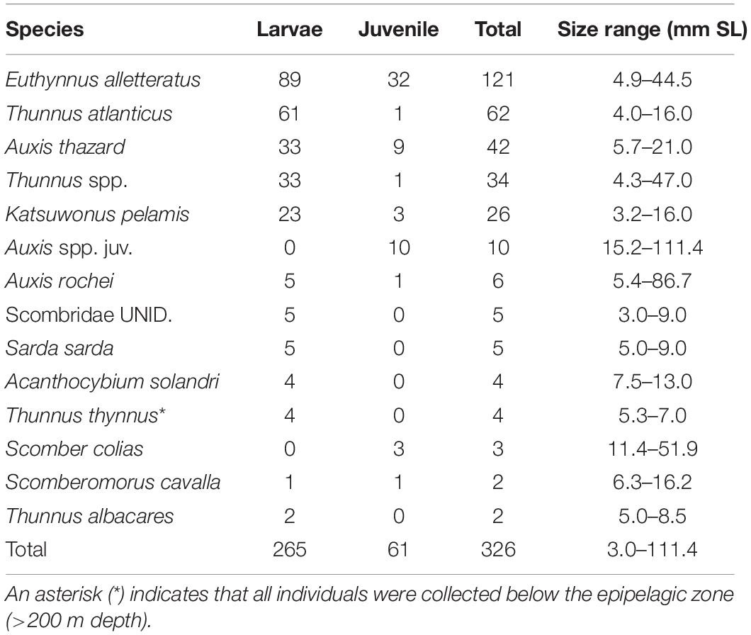
Table 1. Counts and size range of scombrid specimens caught in quantitative tows from the surface to 1500 m depth.

TABLE 2

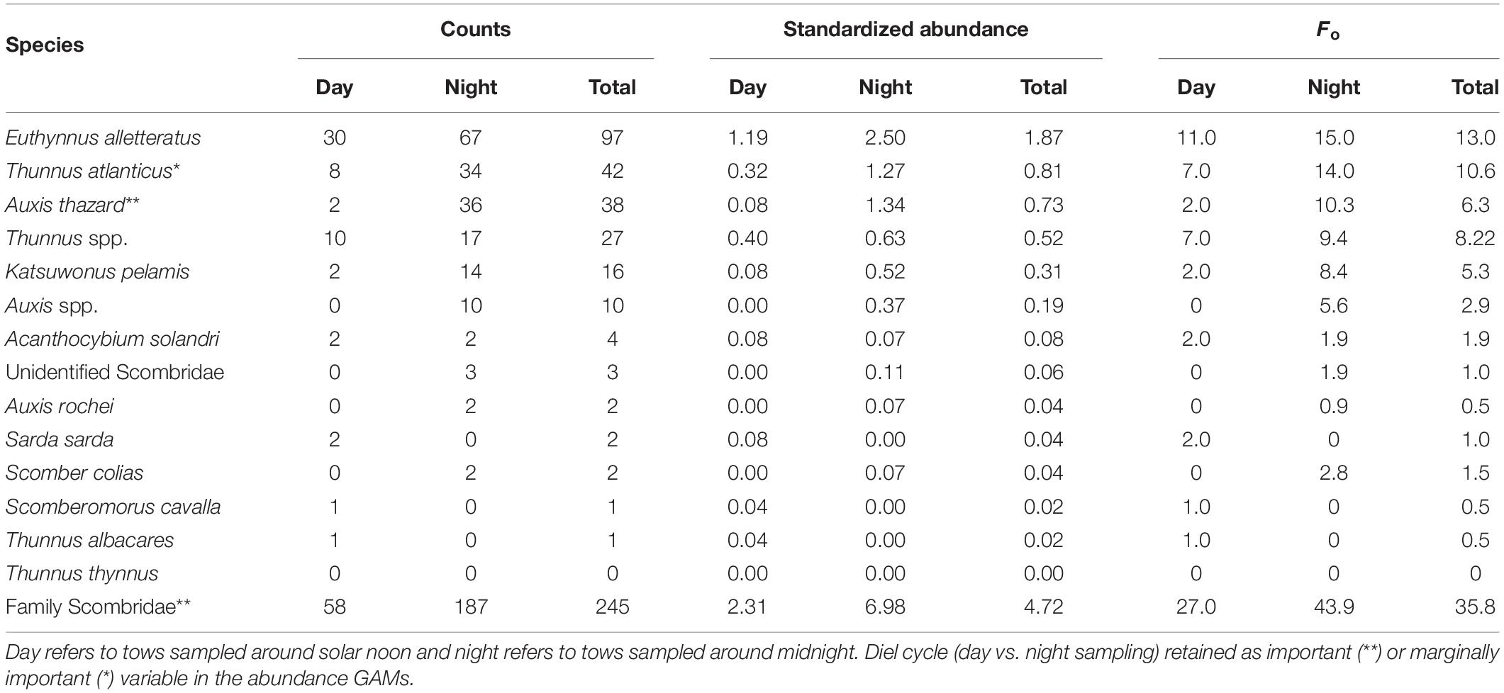
Table 2. Total standardized abundance (no. ind. 10^–5 m^–3) and F_o (%) of scombrid larvae and juveniles collected in the epipelagic zone.

Overall, 85.0% of individuals were identified to species, 13.5% to genus only, and 1.5% to family only. The larval and juvenile scombrid assemblage in this survey comprised 11 of the 16 scombrid species previously reported from the GoM (Richards, 2005). Only four specimens of the endangered T. thynnus were collected, all of which were caught below the epipelagic zone (>200 m depth). One T. thynnus larva (6.4 mm SL) was collected on August 25, 2011, outside of their known spawning time period.

Scombrid specimens ranged in size from 3.0 to 111.4 mm SL, with an average size of 11.8 mm SL (Table 1 and Figure 1). The smallest identifiable larval scombrid was Katsuwonus pelamis (3.2 mm SL) and the largest was a juvenile Auxis sp. (111.4 mm SL). Most specimens were collected in the late-larval phase (81.3%), with 18.7% of individuals in the juvenile stage.

FIGURE 1

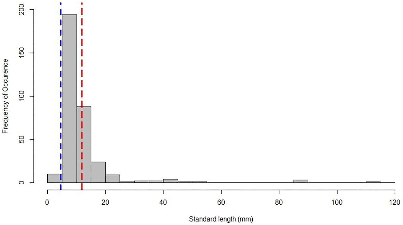
Figure 1. Size-frequency plot of larval and juvenile scombrids collected from January to September in 2011, with the average-sized specimen indicated by the red dashed line. The blue dashed line signifies the average-sized specimen collected on DEEPEND’s complementary ichthyoplankton cruises (4.6 mm SL; Cornic et al., 2018).

Epipelagic Abundances and F_o

The most-abundant species collected in epipelagic zone from January to September 2011 were Euthynnus alletteratus, Thunnus atlanticus, and Auxis thazard, comprising approximately 72% of the total abundance of scombrids captured (Table 2). Euthynnus alletteratus was the most-abundant species caught (n = 97; 1.87 ind. 10^–5 m^–3), accounting for c. 40% of the total scombrids captured. Thunnus atlanticus, the most common true tuna species (Thunnus spp.) in our samples, was the second-most abundant species overall (n = 42; 0.81 ind. 10^–5 m^–3), comprising c. 17% of the captured scombrids. Thunnus atlanticus, along with the other Thunnus species, comprised c. 29% of the scombrid abundance (n = 70; 1.35 ind. 10^–5 m^–3). Auxis thazard was the third-most abundant species collected (n = 38; 0.73 ind. 10^–5 m^–3) in this study.

Scombrids collected in the epipelagic zone were collected in higher abundances at night (6.98 ind. 10^–5 m^–3) than during the day (2.31 ind. 10^–5 m^–3; Table 2). The abundance estimate of E. alletteratus derived from night samples (2.50 ind. 10^–5 m^–3) was twice that from day samples (1.19 ind. 10^–5 m^–3), while T. atlanticus abundance estimates exhibited a four-fold increase from day (0.32 ind. 10^–5 m^–3) to night sampling (1.27 ind. 10^–5 m^–3). Auxis thazard and Katsuwonus pelamis were also caught at higher rates at night (1.34 and 0.52 ind. 10^–5 m^–3, respectively) than during the day (both 0.08 ind. 10^–5 m^–3).

The most-abundant species were also collected at higher F_o at night than during the day in the epipelagic zone (Table 2). There was 27.0% F_o during the day and 43.9% at night for the family Scombridae. Euthynnus alletteratus had a higher F_o at night, occurring in 11.0% of the day trawls and 15.0% of the night trawls. Thunnus atlanticus exhibited a F_o in 7.0% of the day trawls and 14.0% of the night trawls. Auxis thazard F_o increased between day and night samples, with 2.0% of the day trawls and 10.3% of the night trawls. Katsuwonus pelamis exhibited a F_o in 2.0% of day trawls and 8.4% of night trawls. The remaining, rare-event species and taxa did not exhibit higher nighttime abundances or occurrences, though less than five individuals were collected from each of these species in the epipelagic zone (Table 2).

Spatiotemporal Distributions: Generalized Additive Models

The fitted GAM modeling the total abundance of Scombridae included Julian date, water mass, diel cycle, and distance to the nearest 200-m isobath as important explanatory variables (Table 3). Overall, abundances began to increase in April and May and peaked in August (Figures 2A,C). More individuals were caught in CW (Figures 2D,F), further from the shelf break (Figures 2G,H), and at nighttime (Figures 2I,J). The fitted GAM modeling Scombridae occurrences included Julian date as an important variable, and water mass as a marginally important variable (Table 3). Results aligned with the abundance GAMs, in which there was a higher probability of catching scombrids later in the year (Figures 2B,C) and in CW (Figures 2E,F).

TABLE 3

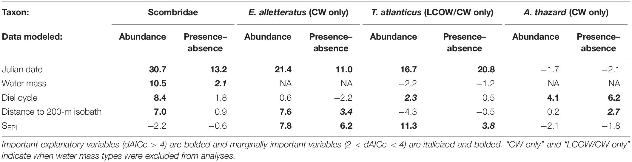
Table 3. dAICc values of abundance and presence–absence GAMs after dropping each explanatory variable for Scombridae, Euthynnus alletteratus, Thunnus atlanticus, and Auxis thazard.

FIGURE 2

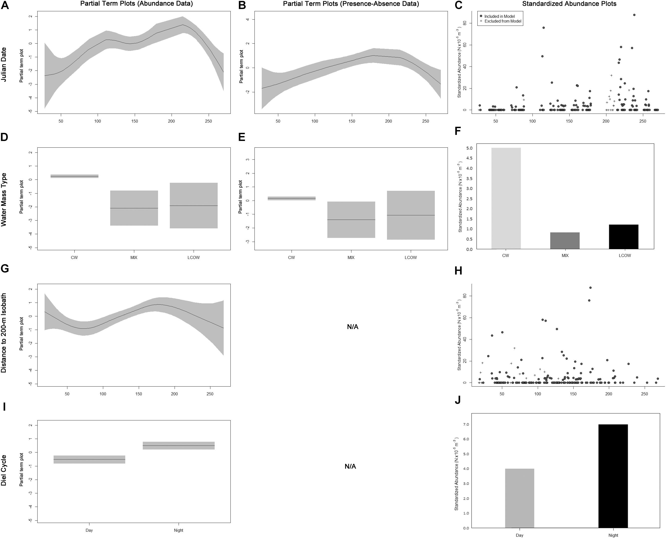
Figure 2. Term plots for the best-fitting models for Scombridae data fitted to the abundance data (A,D,G,I) and presence–absence data (B,E). Standardized abundance plots (C,F,H,J) are also presented for all important and marginally important variables. Data that had to be excluded from the model due to missing MOCNESS sensor data are indicated by crosses.

Euthynnus alletteratus was only captured in CW; therefore, E. alletteratus GAMs were only fitted to samples collected from CW, and water mass was removed as a variable from the full models. The fitted GAM modeling the abundance of E. alletteratus contained Julian date, S_EPI, and distance to the nearest 200-m isobath as important explanatory variables (Table 3). Euthynnus alletteratus abundances increased throughout the year, with the highest peak occurring around August (Figures 3A,C). Higher abundances were associated with lower S_EPI (Figures 3D,F), in which catches occurred in waters as fresh as 29.47 and most specimens (n = 59) were collected in S_EPI < 34. More individuals were also collected nearer to the shelf break (19.79 to 227.31 km from the shelf break), with the majority of specimens within 180 km of the isobath (n = 62, Figures 3G,I). The fitted GAM modeling E. alletteratus occurrences identified Julian date and S_EPI as important, and distance to the nearest 200-m isobath as marginally important variables (Table 3). The presence–absence model results were similar to the abundance GAMs, in which individuals were more likely to be caught later in the year (Figures 3B,C), in low S_EPI (Figures 3E,F), and nearer to the shelf break (Figures 3H,I).

FIGURE 3

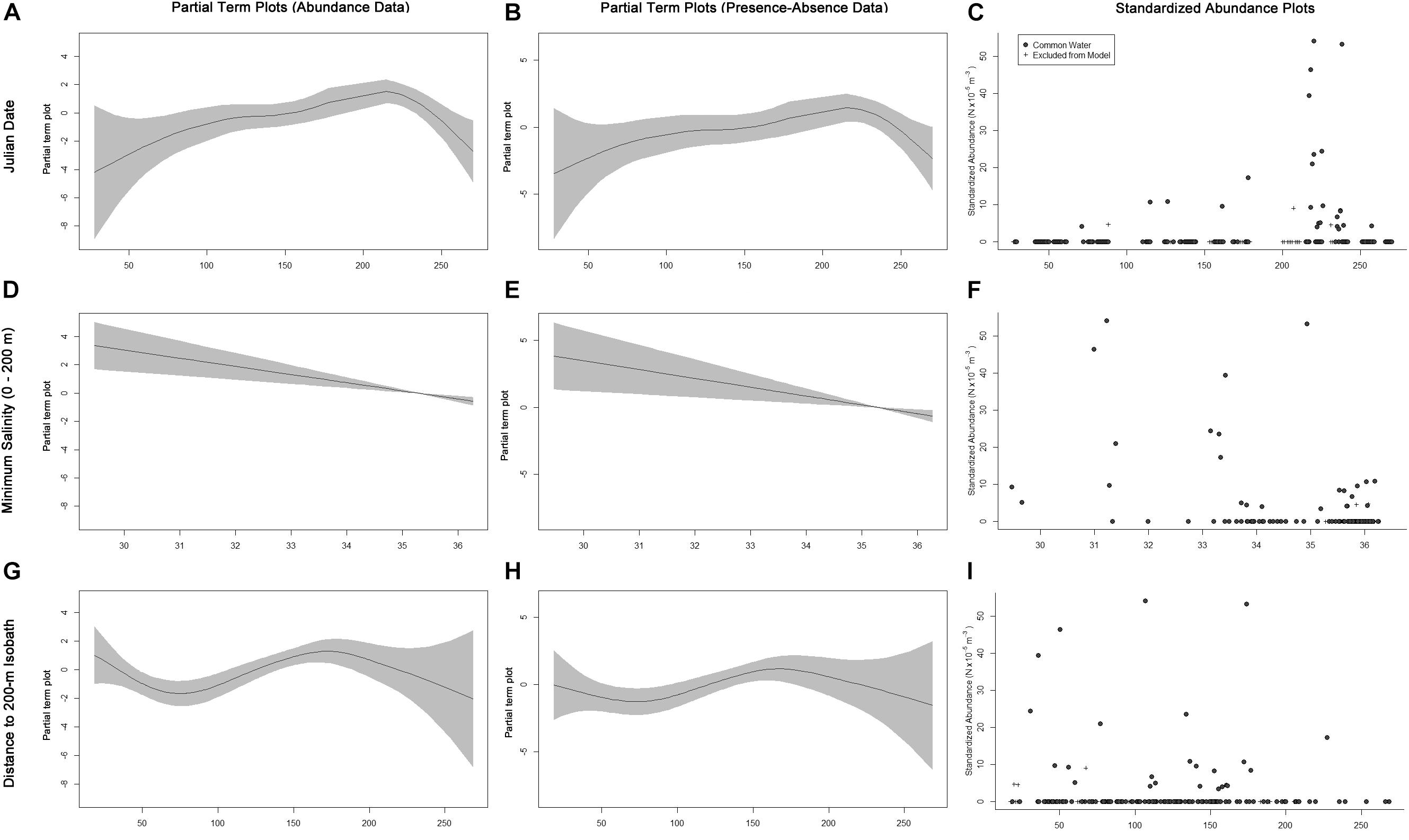
Figure 3. Term plots for the best-fitting models for Euthynnus alletteratus data fitted to the abundance data (A,D,G) and presence–absence data (B,E,H). Standardized abundance plots (C,F,I) are also presented for all important and marginally important variables. Data that had to be excluded from the model due to missing MOCNESS sensor data are indicated by crosses.

Only one Thunnus atlanticus specimen was collected in MIX water; thus, the GAMs fitted to T. atlanticus only included samples from LCOW and CW. The fitted GAM modeling the total abundance of T. atlanticus included Julian date and S_EPI as important and diel cycle as marginally important variables (Table 3). Thunnus atlanticus abundances showed higher abundances beginning in June and continuing through September (Figures 4A,C). High abundances were positively correlated with higher S_EPI (Figures 4D,F), with catches occurring only in S_EPI between 33.82 and 36.13. The majority of specimens (n = 37, 88%) were caught in water with S_EPI > 35. More individuals were collected at nighttime (Figures 4G,H). The fitted GAM modeling T. atlanticus occurrences included Julian date as important and S_EPI as marginally important variables (Table 3). The presence–absence model results were similar to the abundance GAMs, in which there was a higher probability of catching T. atlanticus from June to September (Figures 4B,C) and in higher S_EPI (Figures 4E,F).

FIGURE 4

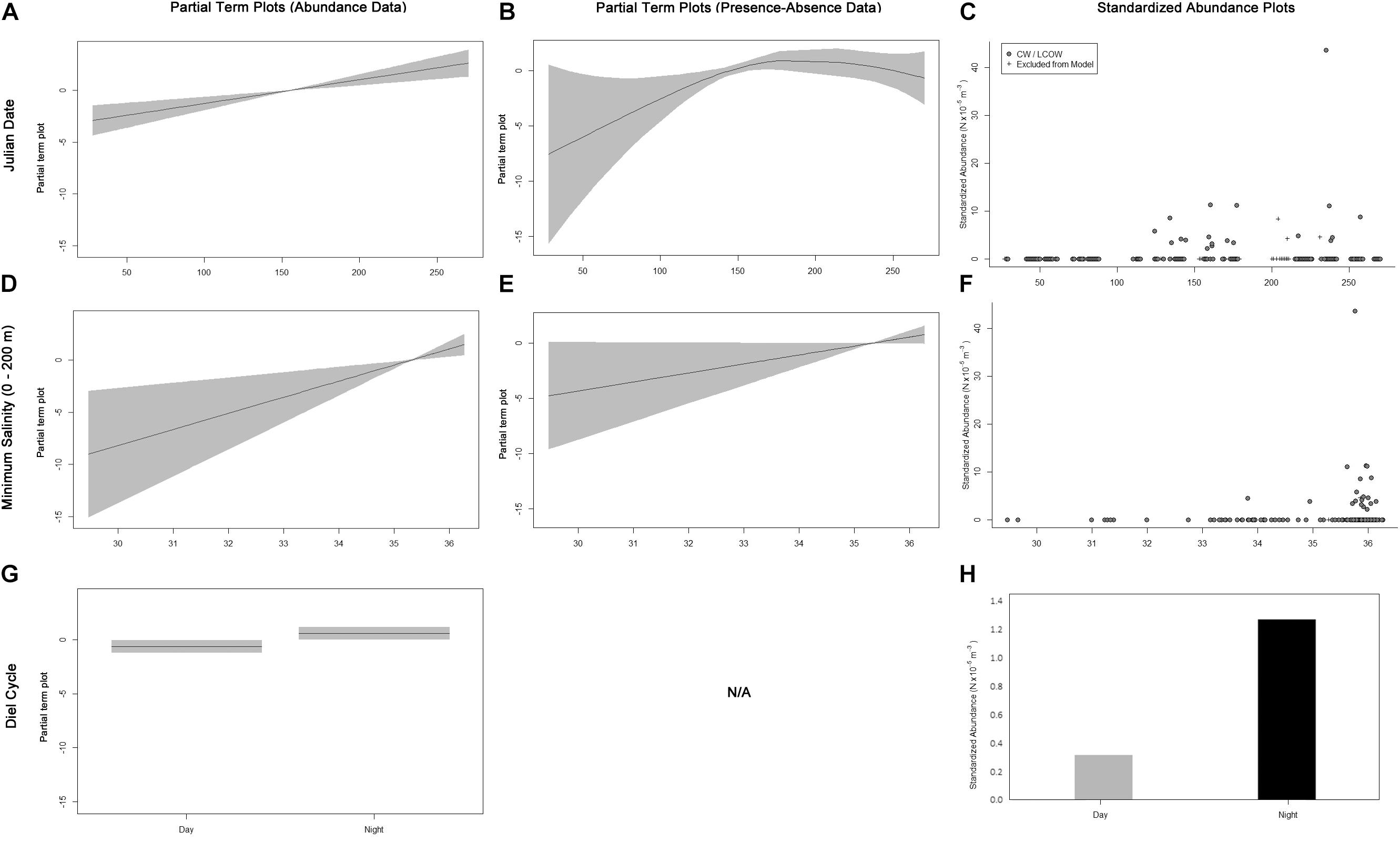
Figure 4. Term plots for the best-fitting models for Thunnus atlanticus data fitted to the abundance data (A,D,G) and presence–absence data (B,E). Standardized abundance plots (C,F,H) are also presented for all important and marginally important variables. Data that had to be excluded from the model due to missing MOCNESS sensor data are indicated by crosses.

Auxis thazard was only collected in CW; therefore, only samples from CW were included, and the water mass variable was removed from the full models. The fitted GAM modeling the total A. thazard abundance included diel cycle as an important variable (Table 3), with more individuals collected at night (Figures 5A,C). The fitted GAM modeling A. thazard occurrences included diel cycle as important (Table 3) and distance to the nearest 200-m isobath as marginally important variables (Table 3). The presence–absence model results were similar to the abundance GAMs, in which there was a higher probability of catching A. thazard at night (Figures 5B,C) and mid-shelf as an outer neritic species (Figures 5D,E).

FIGURE 5

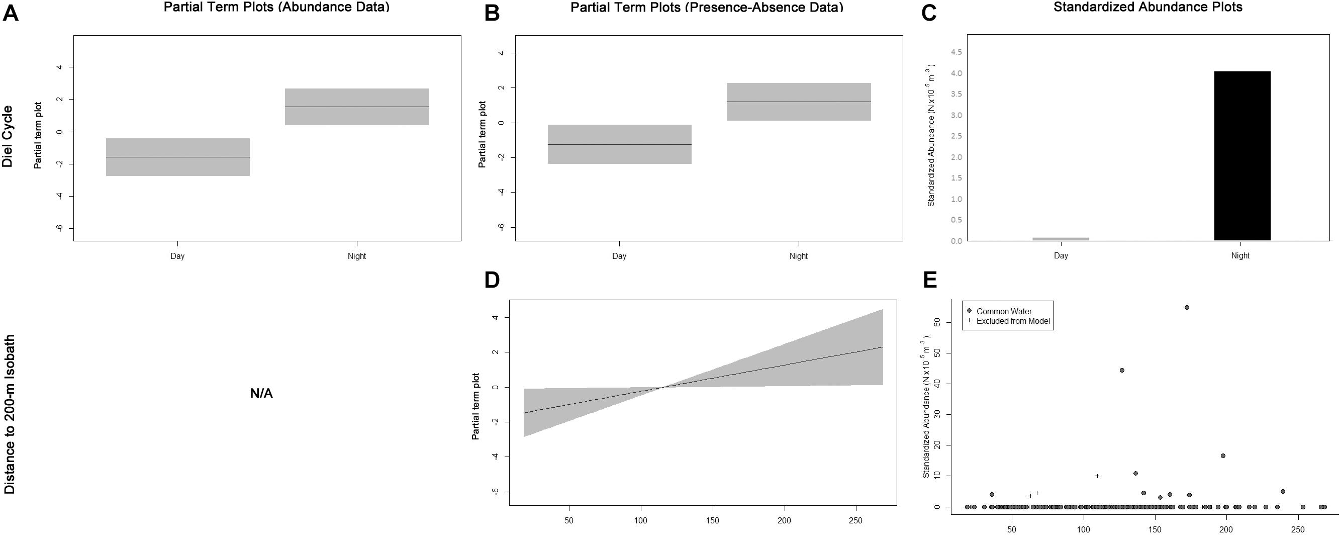
Figure 5. Term plots for the best-fitting models for Auxis thazard data fitted to the abundance data (A) and presence–absence data (B,D). Standardized abundance plots (C,E) are also presented for all important and marginally important variables. Data that had to be excluded from the model due to missing MOCNESS sensor data are indicated by crosses.

Discussion

Assemblage Structure and Spatiotemporal Distributions

The present study identified the faunal composition and assemblage structure of late-larval and juvenile scombrids throughout the northern GoM and characterized the spatiotemporal distributions of the most-abundant species in epipelagic waters with respect to geographic location, oceanographic features, and temporal change.

Of the 16 scombrid species that inhabit the GoM, 11 species were collected in the present study. The collection of a high proportion of the species that occur in the GoM is likely a function of the continuous surveying method, the longevity of sampling (9-month uninterrupted sampling period, January–September 2011), and the day/night sampling during these cruise series. The advantage of continuously sampling a large spatial area and environmental conditions over a relatively long time period (9 months) increases the likelihood of collecting a variety of species. These large-scale faunal surveys remain extremely rare in pelagic research; thus, the data presented here are both robust and unique.

The dominant tunas of the Tribe Thunnini that occur in the GoM, primarily Thunnus spp., but also Auxis spp., Euthynnus alletteratus, and Katsuwonus pelamis (Richards et al., 1993; Richardson et al., 2010; Habtes et al., 2014; Cornic et al., 2018), were collected in the present study. Thunnus spp. have consistently been reported as the dominant tuna taxon in ichthyoplankton surveys during the GoM’s spring and summer months (Richards et al., 1993; Lindo-Atichati et al., 2012; Cornic et al., 2018), although, the most-abundant taxa captured in this study were small-bodied tuna species: E. alletteratus, T. atlanticus, and Auxis thazard. It is possible that the preponderance of small-bodied taxa in our study relative to previous studies reflects higher survivorship of their early life history stages than larger-bodied tunas, the latter showing a more r-selected reproductive strategy (sensu Pianka, 1970).

Scombrids collectively preferred CW conditions over the warmer and high SSHA waters within the MIX water and LCOW. Of the three most-abundant species, T. atlanticus was the only species collected in LCOW in addition to CW. Lindo-Atichati et al. (2012) found that larval E. alletteratus had similar abundances between CW and LCOW in the GoM, larval Auxis spp. (i.e., A. thazard and A. rochei) were found along the boundaries of anticyclonic features and within the GoM’s CW, and Thunnus spp. and T. thynnus larvae were more abundant in the boundaries of anticyclonic features in the GoM. It has been proposed that year-round inhabitant species (e.g., T. atlanticus) have broader habitat preferences in the GoM than T. thynnus and are better able to tolerate warm features, such as the Loop Current and warm eddies (Muhling et al., 2010; Teo and Block, 2010; Lindo-Atichati et al., 2012). Variability in the abundances within CW can also relate to smaller-scale oceanographic features (e.g., cyclonic eddies) in addition to changes in environmental variables that were investigated in this study (i.e., S_EPI, Chl a).

Abundance and presence–absence GAMs additionally identified a coastal group (E. alletteratus and A. thazard) and an oceanic group, represented by T. atlanticus. The coastal group was associated with more productive continental shelf and slope environments (low S_EPI, high Chl a, nearer to shelf break), while the oceanic group was associated with offshore, oligotrophic habitats (high S_EPI, low Chl a, further from shelf break).

Nearshore environments and areas with high terrestrial runoff are associated with low S_EPI and high Chl a, which relates to the coastal life history traits of E. alletteratus and A. thazard. Euthynnus alletteratus preferred nearshore environments with lower S_EPI (<34), and A. thazard was characterized as an outer neritic species, as it preferred areas along the outer shelf break. Maximum freshwater discharge into the GoM from the Mississippi River occurs in the spring. The plume is characterized by lower S_EPI and higher Chl a. Their preference of nearshore environments with lower S_EPI suggests that areas with high freshwater inflow are suitable habitats for the larvae and small-bodied juvenile size classes of coastal tunas. As nutrients increase from runoff, primary and secondary production increase, and in turn provide food for larvae along the continental shelf regions (Le Fevre, 1986; Grimes and Finucane, 1991; Grimes and Kingsford, 1996). Thus, riverine discharge likely maximizes growth and survival of E. alletteratus and A. thazard early life stages.

The GoM experienced a highly productive year in 2011 (Muller-Karger et al., 2015), with high Chl a waters and low S_EPI, especially along the coast due to increased runoff from the Mississippi River. These favorable and highly productive conditions in the nearshore environment could contribute to the numerical dominance of E. alletteratus and A. thazard observed in this study.

Offshore waters typically exhibit higher S_EPI and low to moderate Chl a. Larval and juvenile T. atlanticus were collected in offshore waters, with higher S_EPI. Spawning in these open-ocean environments increases the initial survival of their eggs and larvae due to the reduction in ichthyoplankton predators compared to the coastal waters, though this may be offset at exogenous feeding by lower food supply. Similar to adult T. atlanticus, adult T. thynnus also spawn in waters with lower surface Chl a (0.10–0.16 mg m^–3) and higher S_EPI (35.5–37.0; Teo et al., 2007). Other pelagic fishes (e.g., swordfish, Xiphias gladius) also utilize warm, oligotrophic waters for spawning (Teo et al., 2007). Some tuna species have larvae adapted to living in these nutrient-poor environments, utilizing appendicularians for food at the beginning of their piscivorous early life stages (Llopiz et al., 2010). It appears that T. atlanticus early life stages prefer to remain in, and have adapted to, living in areas with increased S_EPI and decreased Chl a.

Cornic et al. (2018) also found that T. atlanticus larvae preferred intermediate to high salinities, ranging from 31 to 36, and identified T. atlanticus as the most common true tuna from surveys conducted in the northern GoM (June and July, 2007 to 2010), accounting for 81% of the Thunnus larvae. High abundances of T. atlanticus also observed in the present study suggest that T. atlanticus is the most-abundant true tuna species inhabiting the GoM.

Temporal changes in scombrid abundances were associated with species-specific spawning preferences, in which high peaks in abundances in April, June, and August were influenced by A. thazard, E. alletteratus, and T. atlanticus, respectively.

An increase in abundance in April (around day 115) was dominated by A. thazard specimens. Auxis thazard spawns at sea surface temperatures (SSTs) of 21.6 to 30.5°C, with mass spawning between 25.0 and 26.0°C (Rudomiotkina, 1984; ICCAT, 2016a). The SSTs in April reached the massive spawning temperature range for A. thazard, which provides an explanation for the high observed abundances of this species.

Euthynnus alletteratus produces several spawning batches per reproductive season (Chur, 1973; Rudomiotkina, 1986; ICCAT, 2016a), which explains the numerous peaks in abundances throughout the year (increasing from March to September and a large peak in August). Additionally, spawning occurs when waters are the warmest in the GoM (preferably greater than 25°C), from April to November. Surface temperatures reached about 25°C in April, when spawning begins to occur for this species (Chur, 1973; Rudomiotkina, 1986; ICCAT, 2016a). Thus, the temporal changes observed through this 9-month survey influenced the high abundance of E. alletteratus in the GoM.

For T. atlanticus, spawning in the GoM typically occurs between June and September (Collette, 2010), particularly when SSTs reach 27°C (Juarez and Frías, 1986). Water temperatures reached 27°C in June when abundances strongly increased (with highest catches in August), aligning with the previously reported spawning preferences. A few specimens were collected in September, as temperatures began to drop. These patterns relate to the high abundances noted in the ichthyoplankton surveys conducted by Cornic and Rooker (2018) in June and July in 2011.

In addition to the three most-abundant taxa, Katsuwonus pelamis, Auxis rochei, Sarda sarda, Acanthocybium solandri, Thunnus thynnus, Scomber colias, and Thunnus albacares were collected in the present study. Some species, such as the non-resident T. thynnus, were rare in these collections, most likely due to their restricted and shorter spawning seasons in the GoM compared to other resident spawners (ICCAT, 2016a). However, it is interesting to note the collection of a 6.4 mm SL T. thynnus specimen in late August. A comparison with estimated growth rates suggests that the specimen was approximately 9 days old (Malca et al., 2017), indicating that this specimen was spawned in mid-August. While this is an observation of only a single specimen, our findings suggest that the spawning period for T. thynnus, which is currently estimated as occurring between April and June in the GoM, may extend through to August in a limited fashion. Moreover, all T. thynnus larvae were collected below 200 m depth, which indicates a level of connectivity between ‘classic’ epipelagic fishes and deeper pelagic waters over the course of development. Conducting additional larval surveys outside of the “typical” spawning period would help elucidate the extent to which spawning occurs at other times of year in this highly valuable species.

This study highlights the value of large-spatiotemporal scale surveys of oceanic ecosystems such as the GoM, given that scombrid species spawn at different times throughout the year and under different environmental conditions. These large-scale and long-term surveys provide information on the variance in the ecology of species that inhabit an area, can identify commonalities among the faunal assemblage overtime (among years and/or months), and can highlight typical and rare species occurrences in a region.

Size Classes

The 10-m² MOCNESS (3-mm mesh) primarily caught large larval and small juvenile scombrids. The average size specimen collected in this study (11.8 mm SL) was greater than other ichthyoplankton surveys in the GoM, such as Muhling et al. (2012) that collected larvae between 2.5 and 5.0 mm SL and DEEPEND’s complementary ichthyoplankton cruises that collected an average-sized specimen of 4.6 mm SL (Cornic and Rooker, 2018).

The MOCNESS is a larger gear type compared to bongo and neuston nets (with mesh sizes ranging from 335 to 1200 μm) that are typically used in ichthyoplankton surveys to catch small larvae (Richards et al., 1984; Lindo-Atichati et al., 2012; Habtes et al., 2014; Cornic et al., 2018). All else being equal, avoidance is a function of mouth size and extrusion is a function of mesh size (MacLennan, 1992). The larger mouth area, mesh sizes, and faster tow speeds of the MOCNESS ostensibly reduce the ability of these larger larvae and small juveniles to avoid the gear, and in turn, these larger nets are more effective at capturing larger fishes (Kashkin and Parin, 1983). Thus, this study collected fewer planktonic larvae compared to other ichthyoplankton surveys, as smaller individuals were extruded through the MOCNESS’s larger mesh, and in turn, the assemblages of larger larvae and small juveniles were represented.

The larger individuals collected in this study, existing in a higher Reynold’s number environment than small larvae, have increased swimming abilities and mobility due to the development of locomotive features and the need to sustain their high energetic needs and high metabolic costs. More mobile individuals can actively locate and capture prey more easily, adjust their distributions within the water column (horizontally and vertically), and, in turn, increase their growth and survival rates (Werner and Gilliam, 1984). Understanding the assemblage structure and distributional patterns of these larger larvae and small juvenile size classes are critical for fisheries management and conservation efforts as these size classes represent the cohort that has survived the high-mortality “gauntlet” experienced by small larvae (Anonymous, 1984; ICCAT, 2016a).

Comparison of the relative dominance between sampling strategies in the same place and at similar times of year can also potentially inform taxon-specific mortality rates at different size classes. While larval assemblages are used as a proxy for predicting spawning stock biomass, late-larval and juvenile assemblages should also be used to predict future stocks, as these individuals provide a more accurate representation of the surviving year classes of scombrids in the GoM, and subsequently, those individuals (and genetic lineages) that have a higher chance of persisting to adulthood. It is an advantage to use multiple sampling methods (e.g., neuston nets, bongos, MOCNESS) in order to gain a more complete analysis of scombrid ecology and size class assemblages.

Diel Catchability in the Epipelagial

It is important to understand diel differences in day and night catch rates during surveying, as quantitative data are used in scombrid stock assessments. In this study, scombrid early life stages were collected at higher abundances and higher frequencies at night than during the daytime in the epipelagic zone. Increased catches at night are most likely a result of net detection and avoidance during the daytime (Davis et al., 1990). Diel differences in feeding activity also influence catch rates. Most larval and juvenile scombrids feed during the day (Young and Davis, 1990; Tanabe, 2001; Morote et al., 2008), when they are more active. Sensing the nets, and swimming away from them, is more likely to occur during the day when early life stages are more active. Thus, higher catches at night may be related to lower activity levels, decreased swimming activity, and reduced ability to visually detect and avoid nets (Takashi et al., 2006).

While daytime sampling may be appropriate for smaller larvae, it is evident that for the size classes collected in this study (larger larvae and smaller juveniles) it is more beneficial to sample at night in order to collect a more accurate representation of abundance in the epipelagic. These larger individuals are able to actively move across larger spatial scales, and their distributions are more likely to be behavioral compared to a planktonic existence exhibited by larvae.

There is additional supporting evidence of higher capture rates of larval tuna at night. Cornic and Rooker (2018) noted an increase in abundances of T. atlanticus prior to sunset and after dawn in the northern GoM, though their sampling protocol did not include night (midnight) sampling, obfuscating comparison to the present study. In the vicinity of Puerto Rico and the Virgin Islands, Hare et al. (2001) collected more K. pelamis larvae at night, but larval T. atlanticus and E. alletteratus abundances were similar between day and night tows. Previous studies involving larval Auxis spp. also observed higher catches at night in the Philippines, Atlantic Ocean, and Pacific Ocean (Wade and Bravo, 1951; Matsumoto, 1959; Strasburg, 1960; Klawe, 1963).

Recognizing catch differences between day and night sampling is important for fisheries management. Results from this study indicate that it is more appropriate to sample the epipelagic zone at night in order to collect quantitative abundance data that more accurately reflect the true abundance of large larvae and smaller juvenile scombrids in an area.

Conclusion

Bongo nets have proven effective at catching smaller larvae, neuston nets effectively catch slightly larger larvae, and hook-and-line sampling catches adults. However, an effective sampling method does not currently exist for sampling these large larvae and small juveniles, and traditional gear types undersample these size classes. Utilizing multiple sampling methods to target tuna early life stages can improve long-term assessments of recruitment, spawning, and stock biomass of tunas. Such large-scale surveys taken over seasonal cycles provide invaluable information regarding spawning, recruitment, and survivorship rates throughout a year. This study provided a cumulative quantitative analysis and more accurate representation of the scombrid cohort that survived the high mortality that is typically experienced by small larvae. It is important to continue exploring additional modifications of sampling methods for these size classes in order to gather ecological data on these poorly studied, small-bodied tuna species.

Scombrids have a wide variety of life history strategies and spatiotemporal distributions that are often dictated by adult spawning and migratory behaviors. Through spawning, adults establish the initial broad distribution of eggs and small larvae, and the larger larvae and small juveniles modify these distributions through their own behavior. Different seasonal and horizontal distributional patterns existed among the species examined in this study. Horizontal distributions were closely linked with physical characteristics of the water column and mesoscale oceanographic features. Oceanic species (Thunnus atlanticus) preferred more oligotrophic habitats (high S_EPI, low Chl a, further distance from shelf break), while coastal species (Euthynnus alletteratus and Auxis thazard) preferred more productive continental shelf and slope environments (low S_EPI, high Chl a, nearer to shelf break).

Overall, this study quantified the habitat preferences of late-larval and juvenile scombrids in the northern GoM. Results from this study demonstrate the partitioning of pelagic habitat by tunas, from late larvae to adults, particularly for small-bodied tuna species (e.g., E. alletteratus and T. atlanticus) that do not have any current stock assessments or management plans in place. By understanding habitat preferences of tuna early life stages, we can protect critical spawning grounds and nursery habitats and aim to improve management and conservation efforts regarding scombrid populations in the GoM.

Data Availability Statement

Data are publicly available through the Gulf of Mexico Research Initiative Information & Data Cooperative (GRIIDC) at https://data.gulfresearchinitiative.org (10.7266/N7VX0DK2). Additional data were sourced from the E.U. Copernicus Marine Service (GLOBAL_ANALYSIS_FORECAST_PHY_001_024), the GEBO_2014 Grid (version 20141103) and NASA’s Ocean Biology Processing Group (10.5067/AQUA/MODIS/L3M/CHL/2018).

Author Contributions

NP and TS designed the study; NP analyzed the samples and organized the database; NP and RM performed the statistical analysis and prepared the figures. All authors contributed to manuscript preparation and revision, and read and approved the submitted version.

Funding

This research was funded in part by the NOAA Office of Response and Restoration and in part by a grant from The Gulf of Mexico Research Initiative (GoMRI).

Conflict of Interest

The authors declare that the research was conducted in the absence of any commercial or financial relationships that could be construed as a potential conflict of interest.

Acknowledgments

The authors would like to thank both the science staff and the crew aboard the R/V Meg Skansi. Additional thanks go to Dr. John Lamkin and Aki Shiroza from NOAA NMFS, Miami, FL, for assisting in the larval identifications. This manuscript includes work that was conducted and samples that were collected as part of the Deepwater Horizon Natural Resource Damage Assessment being conducted cooperatively among academic partners, NOAA, other Federal and State Trustees, and BP.

Supplementary Material

The Supplementary Material for this article can be found online at: https://www.frontiersin.org/articles/10.3389/fmars.2020.00257/full#supplementary-material

Abbreviations

CW, Gulf Common Water classification; LCOW, Loop Current Origin Water classification; MIX, Intermediate Water classification; ONSAP, Offshore Nekton Sampling and Analysis Program; S_EPI, minimum salinity in the epipelagic zone; T_EPI, maximum temperature (° C) recorded in the epipelagic zone.

Footnotes

1. ^ http://marine.copernicus.eu/
2. ^ https://oceancolor.gsfc.nasa.gov/
3. ^ https://www.gebco.net/

References

Anonymous (1984). Meeting of the working group on juveniles tropical tunas. Coll. Vol. Sci. Pap. 21, 1–289.

Google Scholar

Burnham, K., and Anderson, D. (2002). “Model selection and multimodel inference: a practical information-theoretic approach,” in Prediction and the Power Transformation Family, eds R. J. Carroll, and D. Ruppert, (New York, NY: Springer-Verlag).

Google Scholar

Chur, V. (1973). Some biological characteristics of little tuna (Euthynnus alletteratus, Rafinesque, 1810) in the eastern part of the tropical Atlantic. Coll. Vol. Sci. Pap. 1, 489–500.

Google Scholar

Collette, B., and Graves, J. (2019). Tunas and Billfishes of the World. Baltimore: Johns Hopkins University Press.

Google Scholar

Collette, B. B. (2010). “Reproduction and development in epipelagic fishes,” in Reproduction and Sexuality in Marine Fishes: Patterns and Processes, ed. K. S. Cole, (Berkeley: University of California Press).

Google Scholar

Cornic, M., and Rooker, J. R. (2018). Influence of oceanographic conditions on the distribution and abundance of blackfin tuna (Thunnus atlanticus) larvae in the Gulf of Mexico. Fish Res. 201, 1–10. doi: 10.1016/j.fishres.2017.12.015

CrossRef Full Text | Google Scholar

Cornic, M., Smith, B. L., Kitchens, L. L., Bremer, J. R. A., and Rooker, J. R. (2018). Abundance and habitat associations of tuna larvae in the surface water of the Gulf of Mexico. Hydrobiologia 806, 29–46. doi: 10.1007/s10750-017-3330-0

CrossRef Full Text | Google Scholar

Davis, T. L., Jenkins, G. P., and Young, J. W. (1990). Diel patterns of vertical distribution in larvae of southern bluefin, Thunnus maccoyii, and other tuna in the East Indian Ocean. Mar. Ecol. Prog. Ser. 59, 63–74. doi: 10.3354/meps059063

CrossRef Full Text | Google Scholar

Grimes, C. B., and Finucane, J. H. (1991). Spatial distribution and abundance of larval and juvenile fish, chlorophyll and macrozooplankton around the Mississippi River discharge plume, and the role of the plume in fish recruitment. Mar. Ecol. Prog. Ser. 75, 109–119. doi: 10.3354/meps075109

CrossRef Full Text | Google Scholar

Grimes, C. B., and Kingsford, M. J. (1996). How do riverine plumes of different sizes influence fish larvae: do they enhance recruitment? Mar. Freshw. Res. 47, 191–208.

Google Scholar

Habtes, S., Muller-Karger, F. E., Roffer, M. A., Lamkin, J. T., and Muhling, B. A. (2014). A comparison of sampling methods for larvae of medium and large epipelagic fish species during spring SEAMAP ichthyoplankton surveys in the Gulf of Mexico. Limnol. Oceanogr.-Methods 12, 86–101. doi: 10.4319/lom.2014.12.86

CrossRef Full Text | Google Scholar

Hare, J. A., Hoss, D. E., Powell, A. B., Konieczna, M., Peters, D. S., Cummings, S. R., et al. (2001). Larval distribution and abundance of the family Scombridae and Scombrolabracidae in the vicinity of Puerto Rico and the Virgin Islands. Bull. Sea Fish Inst. 2, 13–29.

Google Scholar

Hendriks, A. J. (1999). Allometric scaling of rate, age and density parameters in ecological models. Oikos 86, 293–310.

Google Scholar

Hsieh C-h, Reiss, C. S., Hunter, J. R., Beddington, J. R., May, R. M., and Sugihara, G. (2006). Fishing elevates variability in the abundance of exploited species. Nature 443:859. doi: 10.1038/nature05232

CrossRef Full Text | Google Scholar

ICCAT (2016a). ICCAT Manual. International Commission for the Conservation of Atlantic Tuna. Madrid: ICCAT Publications.

Google Scholar

ICCAT (2016b). Report of the Standing Committee on Research and Statistics (SCRS). Madrid: ICCAT Publications, 1–426.

Google Scholar

Johnston, M., Milligan, R., Easson, C., DeRada, S., Penta, B., and Sutton, T. (2019). An empirically-validated method for characterizing pelagic habitats in the gulf of mexico using ocean model data. Limnol Oceanogr.-Methods 17, 362–375.

Google Scholar

Juan-Jordá, M. J., Mosqueira, I., Cooper, A. B., Freire, J., and Dulvy, N. K. (2011). Global population trajectories of tunas and their relatives. Proc. Natl. Acad. Sci. U.S.A. 108, 20650–20655. doi: 10.1073/pnas.1107743108

CrossRef Full Text | Google Scholar

Juarez, M., and Frías, P. (1986). “Distribución de las larvas de bonito (Kasuwonus pelamis) y falsa albacora (Thunnus atlanticus)(Pisces: Scombridae) en la zona económica de Cuba,” in Actas de la Conferencia ICCAT Sobre el Programa del Año Internacional del Listado, eds P. E. K. Symons, M. Miyake, and G. T. Sakagawa, (Madrid: International Commission for the Conservation of Atlantic Tunas).

Google Scholar

Kashkin, N. I., and Parin, N. V. (1983). Quantitative assessment of micronektonic fishes by nonclosing gear (a review). Biol. Oceanogr. 2, 263–287.

Google Scholar

Klawe, W. L. (1963). Observations on the spawning of four species on tuna (Neothunnus macropterus, Katsuwonus pelamis, Auxis thazard and Euthynnus lineatus) in the Eastern Pacific Ocean, based on the distribution of their larvae and juveniles. Inter.-Am. Trop. Tuna Commun. Bull. 6, 447–540.

Google Scholar

Lang, K. L., Grimes, C. B., and Shaw, R. F. (1994). Variations in the age and growth of yellowfin tuna larvae, Thunnus albacares, collected about the Mississippi River plume. Environ. Biol. Fish 39, 259–270. doi: 10.1007/bf00005128

CrossRef Full Text | Google Scholar

Le Fevre, J. (1986). Aspects of the biology of frontal systems. Adv. Mar. Biol. 23, 163–299. doi: 10.1016/s0065-2881(08)60109-1

CrossRef Full Text | Google Scholar

Lindo-Atichati, D., Bringas, F., Goni, G., Muhling, B., Muller-Karger, F. E., and Habtes, S. (2012). Varying mesoscale structures influence larval fish distribution in the northern Gulf of Mexico. Mar. Ecol. Prog. Ser. 463, 245–257. doi: 10.3354/meps09860

CrossRef Full Text | Google Scholar

Llopiz, J. K., Richardson, D. E., Shiroza, A., Smith, S. L., and Cowen, R. K. (2010). Distinctions in the diets and distributions of larval tunas and the important role of appendicularians. Limnol. Oceanogr. 55, 983–996. doi: 10.4319/lo.2010.55.3.0983

CrossRef Full Text | Google Scholar

MacLennan, D. N. (1992). Fishing gear selectivity: an overview. Fish. Res. 13, 201–204. doi: 10.1016/0165-7836(92)90076-6

CrossRef Full Text | Google Scholar

Majkowski, J. (2007). Global Fishery Resource of Tuna and Tuna-like Species: FAO Fish Tech Pap 54. Rome: FAO.

Google Scholar

Malca, E., Muhling, B., Franks, J., García, A., Tilley, J., Gerard, T., et al. (2017). The first larval age and growth curve for bluefin tuna (Thunnus thynnus) from the Gulf of Mexico: comparisons to the Straits of Florida, and the Balearic Sea (Mediterranean). Fish. Res. 190, 24–33. doi: 10.1016/j.fishres.2017.01.019

CrossRef Full Text | Google Scholar

Matsumoto, W. M. (1959). Descriptions of Euthynnus and Auxis Larvae from the Pacific and Atlantic Oceans and adjacent seas: Fish Bull, Book 50. Copenhagen: Carlsberg Foundation.

Google Scholar

Matthews, F. D., Damaker, D. M., Knapp, L. W., and Collette, B. (1977). Food of Western North Atlantic tunas (Thunnus) and Lancetfishes (Alepisaurus). Silver Spring: Department of Commerce, National Oceanic and Atmospheric Administration, National Marine Fisheries Service.

Google Scholar

McEachran, J. D., and Fechhelm, J. D. (1998). Fishes of the Gulf of Mexico, Myxiniformes to Gasterosteiformes, Vol. 1. Austin: University of Texas Press.

Google Scholar

Molinari, R. L. (1980). Current variability and its relation to sea-surface topography in the Caribbean Sea and Gulf of Mexico. Mar. Geod 3, 409–436. doi: 10.1080/01490418009388006

CrossRef Full Text | Google Scholar

Morote, E., Olivar, M. P., Pankhurst, P. M., Villate, F., and Uriarte, I. (2008). Trophic ecology of bullet tuna Auxis rochei larvae and ontogeny of feeding-related organs. Mar. Ecol. Prog. Ser. 353, 243–254. doi: 10.3354/meps07206

CrossRef Full Text | Google Scholar

Muhling, B., Roffer, M., Lamkin, J., Ingram, G., Upton, M., Gawlikowski, G., et al. (2012). Overlap between Atlantic bluefin tuna spawning grounds and observed Deepwater Horizon surface oil in the northern Gulf of Mexico. Mar. Pollut. Bull. 64, 679–687. doi: 10.1016/j.marpolbul.2012.01.034

CrossRef Full Text | Google Scholar

Muhling, B. A., Lamkin, J. T., and Roffer, M. A. (2010). Predicting the occurrence of Atlantic bluefin tuna (Thunnus thynnus) larvae in the northern Gulf of Mexico: building a classification model from archival data. Fish. Oceanogr. 19, 526–539. doi: 10.1111/j.1365-2419.2010.00562.x

CrossRef Full Text | Google Scholar

Muller-Karger, F. E., Smith, J. P., Werner, S., Chen, R., Roffer, M., Liu, Y., et al. (2015). Natural variability of surface oceanographic conditions in the offshore Gulf of Mexico. Prog. Oceanogr. 134, 54–76. doi: 10.1016/j.pocean.2014.12.007

CrossRef Full Text | Google Scholar

Nakata, H., Kimura, S., Okazaki, Y., and Kasai, A. (2000). Implications of meso-scale eddies caused by frontal disturbances of the Kuroshio Current for anchovy recruitment. ICES J. Mar. Sci. 57, 143–152. doi: 10.1006/jmsc.1999.0565

CrossRef Full Text | Google Scholar

Nasa Goddard Space Flight Center, Ocean Ecology Laboratory, Ocean Biology Processing Group (2018). Moderate-Resolution Imaging Spectroradiometer (MODIS) Aqua Chlorophyll Data; Reprocessing. Greenbelt, MD: NASA OB. DAAC.

Google Scholar

Olson, D. B., and Backus, R. H. (1985). The concentrating of organisms at fronts: a cold-water fish and a warm-core Gulf Stream ring. J. Mar. Res. 43, 113–137. doi: 10.1357/002224085788437325

CrossRef Full Text | Google Scholar

Pante, E., and Simon-Bouhet, B. (2013). marmap: a package for importing, plotting and analyzing bathymetric and topographic data in R. PLoS ONE 8:e73051. doi: 10.1371/journal.pone.0073051

CrossRef Full Text | Google Scholar

Pianka, E. R. (1970). On r-and K-selection. Am. Nat. 104, 592–597.

Google Scholar

Pruzinsky, N. (2018). Identification and Spatiotemporal Dynamics of Tuna (Family: Scombridae; Tribe: Thunnini) Early Life Stages in the Oceanic Gulf of Mexico. Masters Thesis. Dania, FL: Nova Southeastern University.

Google Scholar

R Core Team (2019). R: A Language and Environment for Statistical Computing. Vienna: R Foundation for Statistical Computing.

Google Scholar

Richards, W. J. (2005). Early Stages of Atlantic Fishes: An Identification Guide for the Western Central North Atlantic, Two, Vol. 2. Boca Raton, FL: CRC Press.

Google Scholar

Richards, W. J., McGowan, M. F., Leming, T., Lamkin, J. T., and Kelley, S. (1993). Larval fish assemblages at the loop current boundary in the gulf of Mexico. Bull. Mar. Sci. 53, 475–537.

Google Scholar

Richards, W. J., Potthoff, T., Kelley, S., McGowan, M. F., Ejsymont, L., Power, J. H., et al. (1984). Larval distribution and abundance of engraulidae, carangidae, clupeidae, lutjanidae, serranidae, coryphaenidae, istiophoridae, xiphiidae and scombridae in the Gulf of Mexico. NOAA Tech. Mem. NMFS SEFC 144, 1–51.

Google Scholar

Richardson, D. E., Llopiz, J. K., Guigand, C. M., and Cowen, R. K. (2010). Larval assemblages of large and medium-sized pelagic species in the Straits of Florida. Prog. Oceanogr. 86, 8–20. doi: 10.1016/j.pocean.2010.04.005

CrossRef Full Text | Google Scholar

Rigby, R. A., and Stasinopoulos, D. M. (2005). Generalized additive models for location, scale and shape. J. R. Stat. Soc. Ser. C (Appl. Stat.) 54, 507–554.

Google Scholar

Rooker, J. R., Kitchens, L. L., Dance, M. A., Wells, R. D., Falterman, B., and Cornic, M. (2013). Spatial, temporal, and habitat-related variation in abundance of pelagic fishes in the Gulf of Mexico: potential implications of the Deepwater Horizon Oil Spill. PLoS ONE 8:e76080. doi: 10.1371/journal.pone.0076080

CrossRef Full Text | Google Scholar

Rudomiotkina, G. (1984). New data on reproduction of Auxis spp. In the Gulf of Guinea. Collect. Vol. Sci. Pap. 20, 465–468.

Google Scholar

Rudomiotkina, G. (1986). Data on reproduction of Atlantic black skipjack in the tropical West African water. Collect Vol. Sci. Pap. ICCAT 25, 258–261.

Google Scholar

Scott, G. P., Turner, S. C., Churchill, G. B., Richards, W. J., and Brothers, E. B. (1993). Indices of larval bluefin tuna, Thunnus thynnus, abundance in the Gulf of Mexico; modelling variability in growth, mortality, and gear selectivity. Bull. Mar. Sci. 53, 912–929.

Google Scholar

Strasburg, D. W. (1960). Estimates of larval tuna abundance in the central Pacific. Fish. Bull. 60, 231–255.

Google Scholar

Sutton, T. T., Cook, A. B., Moore, J., Frank, T., Judkins, H., Vecchione, M., et al. (2016). Inventory of Gulf Oceanic Fauna Data Including Species, Weight, and Measurements. Meg Skansi cruises from Jan. 25 – Sept. 30, 2011 in the Northern Gulf of Mexico. Distributed by: Gulf of Mexico Research Initiative Information and Data Cooperative (GRIIDC). Christi: Harte Research Institute, Texas A&M University-Corpus.

Google Scholar

Takashi, T., Kohno, H., Sakamoto, W., Miyashita, S., Murata, O., and Sawada, Y. (2006). Diel and ontogenetic body density change in Pacific bluefin tuna, Thunnus orientalis (Temminck and Schlegel), larvae. Aquacult. Res. 37, 1172–1179. doi: 10.1111/j.1365-2109.2006.01544.x

CrossRef Full Text | Google Scholar

Tanabe, T. (2001). Feeding habits of skipjack tuna Katsuwonus pelamis and other tuna Thunnus spp. juveniles in the tropical western Pacific. Fish. Sci. 67, 563–570. doi: 10.1046/j.1444-2906.2001.00291.x

CrossRef Full Text | Google Scholar

Teo, S. L., and Block, B. A. (2010). Comparative influence of ocean conditions on yellowfin and Atlantic bluefin tuna catch from longlines in the Gulf of Mexico. PLoS ONE 5:e10756. doi: 10.1371/journal.pone.0010756

CrossRef Full Text | Google Scholar

Teo, S. L., Boustany, A. M., and Block, B. A. (2007). Oceanographic preferences of Atlantic bluefin tuna, Thunnus thynnus, on their Gulf of Mexico breeding grounds. Mar. Biol. 152, 1105–1119. doi: 10.1007/s00227-007-0758-1

CrossRef Full Text | Google Scholar

Wade, C. B., and Bravo, P. (1951). Larvae of tuna and tuna-like fishes from Philippine waters. Fish Bull 51, 455–485.

Google Scholar

Werner, E. E., and Gilliam, J. F. (1984). The ontogenetic niche and species interactions in size-structured populations. Annu. Rev. Ecol. Syst. 15, 393–425. doi: 10.1146/annurev.es.15.110184.002141

CrossRef Full Text | Google Scholar

Wiebe, P., Morton, A., Bradley, A., Backus, R., Craddock, J., Barber, V., et al. (1985). New development in the MOCNESS, an apparatus for sampling zooplankton and micronekton. Mar. Biol. 87, 313–323. doi: 10.1007/bf00397811

CrossRef Full Text | Google Scholar

Young, J. W., and Davis, T. L. (1990). Feeding ecology of larvae of southern bluefin, albacore and skipjack tunas (Pisces: Scombridae) in the eastern Indian Ocean. Mar. Ecol. Prog. Ser. 61, 17–29. doi: 10.3354/meps061017

CrossRef Full Text | Google Scholar

Zuur, A. F., Ieno, E. N., and Elphick, C. S. (2010). A protocol for data exploration to avoid common statistical problems. Methods Ecol. Evol. 1, 3–14. doi: 10.1111/j.2041-210x.2009.00001.x

CrossRef Full Text | Google Scholar

Zuur, A. F., Ieno, E. N., Walker, N., Saveliev, A. A., and Smith, G. M. (2009). Mixed Effects Models and Extensions in Ecology with R. Berlin: Springer Science & Business Media.

Google Scholar