Metabolic Responses of Subtropical Microplankton After a Simulated Deep-Water Upwelling Event Suggest a Possible Dominance of Mixotrophy Under Increasing CO2 Levels

1. Introduction

The global economy, based on the combustion of fossil resources, has caused the increase in anthropogenic carbon dioxide (CO₂) emissions over the past 250 years, resulting in atmospheric pCO₂ values that currently exceed 400 μatm, the highest level the planet has experienced in the last 800,000 years. Furthermore, atmospheric CO₂ keeps increasing up to one-order-of-magnitude faster than it increased over the previous millions of years (Doney and Schimel, 2007). Oceans are taking up nearly one third of this CO₂, impacting seawater carbonate chemistry, and causing ocean acidification (Doney et al., 2009). Even if these changes raise photosynthetic carbon fixation (Riebesell et al., 2007), the resulting organic matter may have lower nutritional value to the detriment of the rest of the ocean ecosystem (Doney et al., 2009). Under eutrophic conditions, these changes seem to have different effects. In the most acidified environments, picophytoplankton growth is stimulated, and excreted dissolved organic carbon (DOC) becomes an important fraction of the organic matter. In other cases, increases in the pCO₂ levels do not directly enhance sinking material flux (Paul et al., 2015). Under oligotrophic conditions, respiration (R), potential respiration (Φ), primary production (PP) and chorophyll-a (chl-a) levels remained low in both weakly and highly acidified mesocosms studies (Filella et al., 2018; Hernández-Hernández et al., 2018). When the microplankton community under oligotrophic conditions was given an injection of inorganic nutrients, a phytoplankton bloom was produced. In the most acidified mesocosms, R, Φ, and chl-a were more stimulated, although Φ was highly variable (Filella et al., 2018). Also, during the phytoplankton bloom in Hernández-Hernández et al. (2018), PP rose to a peak and rapidly declined to half of the peak value by the end of the bloom. As the PP peaked and fell, the high CO₂ mesocosms were the most productive, but they did not stand out from the other mesocosms (Hernández-Hernández et al., 2018). After nutrient depletion, the decline in PP continued with higher productivity in the most acidified mesocosms (Hernández-Hernández et al., 2018). Here, we continue these types of mesocosm experiments, focusing on cellular metabolism, to further investigate the impact of rising ocean CO₂ levels on plankton.

Cellular metabolism incorporates enzymatic pathways of both biosynthesis and biodegradation. The biosynthesis pathways (anabolism) are found in both autotrophic and heterotrophic organisms throughout the ocean. However, anabolism based on chlorophyll-based photosynthesis is found only in the ocean's euphotic zone (Mackey et al., 1996). Chl-a, in oceanography has been used as a measure of photoautotroph biomass since the Arctic research of Kreps and Verjbinskaya (1930) and more recently, as an index of PP (Ryther and Yentsch, 1957; Huot et al., 2007; Roesler and Barnard, 2013). Both uses are “first approximations” because there are other factors, including light and nutrients, that, for more accuracy, need to be considered. Here, also as a first approximation, we use chl-a to represent anabolism of the phytoplankton fraction of the euphotic-zone microplankton community.

The other side of metabolism, biodegradation or catabolism, generates energy-rich biomolecules needed in both phases of metabolism. The key catabolic pathway for the generation of the universal biological energy currency is the respiratory electron transport system (ETS) (Gnaiger et al., 2019). Since the 1970's, the ETS has been used to represent potential O₂ consumption rates in different components of the marine ecosystem (Packard, 1971; Packard et al., 1974; Moran et al., 2012; Robinson, 2018; Belcher et al., 2019). As ETS activity regulates adenosine triphosphate (ATP) production, we use it here as a first approximation to represent catabolism in a mixed plankton community.

On an environmental scale, anabolism and catabolism are complementary sides of metabolism, where the principal products of photosynthetic biosynthesis (O₂ and glucose) are the main inputs for cell respiration while the principal product of respiration (CO₂) is the main input for biosynthesis (Nelson and Cox, 2008). In this KOSMOS experiment, Hernández-Hernández et al. (2018), Taucher et al. (2018), and Algueró-Muñiz et al. (2019) monitored the shifts in the community composition during different stages of a phytoplankton bloom, ranging from a mixed community to a photoautotroph-dominated one during the bloom, and then, leading to a heterotroph-dominated community or a mixed one. In this paper, we reasoned that these shifts were likely linked to shifts in the balance between the two sides of metabolism. Specifically, we investigated the feasibility of using the ratio between potential respiration rate (Φ) and chl-a as an index of shifts between these two sides of metabolism. Accordingly, we followed the Φ/chl-a relationship through the temporal evolution of the microplankton community (0.7–50.0 μm) as related to the simulated deep-water upwelling, the subsequent diatom bloom, and the nutrient depletion that occurred in all the mesocosms. In our calculations here, restricted by our seawater sampling of the 0.7–50.0 μm size-fraction, the Φ/chl-a ratio pertains just to the microplankton community, not to the mesozooplankton community (50.0–2000.0 μm).

Our conceptual thinking about the Φ/chl-a ratio is consistent with the thinking of Packard (1985), Martinez et al. (1990), Martinez (1991), and Bangqin et al. (2005), where the Φ/chl-a was used as an index of the relative contribution of the total microplankton respiration to the phytoplankton biomass. These studies examined the variability of this ratio and found that in phytoplankton-dominated zones, such as upwelling systems, ocean fronts or chl-a maximum layers, Φ/chl-a is low (Table 1). In addition, Martinez et al. (1990) and Martinez (1991) found that outside these areas, the microheterotrophs' contribution to the microplankton is higher, and the Φ/chl-a increases. With regards to the physiologically measured respiration (R) ratioed to chl-a, in euphotic zones, Robinson et al. (2002) found that in both the northern and southern Benguela upwelling systems, the R/chl-a was low [1.7 mg O₂ (mg chl-a)⁻¹], while in three oligotrophic Eastern Boundary Current oceanic provinces, the ratio was high [6.4 mg O₂ (mg chl-a)⁻¹]. The trend is the same for R/chl-a as it is with Φ/chl-a. Given the fact that Φ/chl-a ratio varied with the composition of the microplankton, the first objective of the present study was to characterize the parallel temporal shifts in the Φ/chl-a ratio and the microplankton composition, as seawater conditions change. In addition, we monitored the daily changes (P_N) in the particulate protein (B) of the mesocosms during the whole experiment by following the first derivative of B with respect to time (dB/dt). Then, we used another simple mathematical trick, integration, to detect changes in Φ, chl-a, and B in the microplankton community, with increasing pCO₂ levels. Thus, our second objective was to show how differential and integral analysis can advance data processing by transforming static processes into dynamic ones and by amplifying time-course signals to the point of detectability. The final objective was to document how increasing CO₂ levels impact Φ, chl-a, and B during different stages of a phytoplankton bloom.

TABLE 1

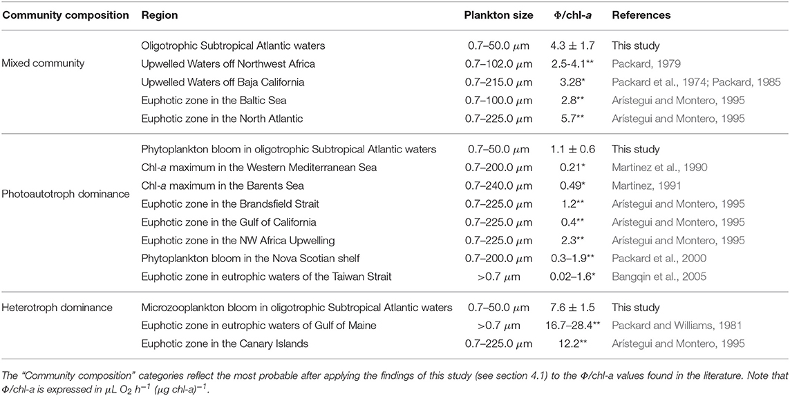
Table 1. Comparison between the Φ/chl-a results in this study, the Φ/chl-a measurements in the literature (highlighted with “*”) and Φ/chl-a values calculated from average Φ and chl-a measurements in the literature, in microplankton communities (highlighted with “**”).

2. Materials and Methods

2.1. Experimental Design

A 55-days in situ KOSMOS (Kiel Offshore Mesocosms for Future Ocean Simulations) experiment was carried out in Gando Bay, on the east coast of Gran Canaria Island (Spain) (27° 55′ 41^′′ N, 15° 21′ 55^′′ W), during autumn 2014 (October-November). Nine 35 m³-mesocosms (M1-M9) (Riebesell et al., 2013), with increasing partial pressure CO₂ (pCO₂) treatments ranging from ambient levels (400 μatm) to 1,200 μatm (see Table 2), were deployed in order to study the physical, ecological, and biogeochemical responses before, during and after a simulated upwelling event. Days of the experiment are designated as T₁,T₂,T₃, up to T₅₅. Note that mesocosm 6 (M6) was lost on T₂₇ due to strong currents in Gando Bay. Consequently, it was excluded from this study. Mesocosms 4 and 9 (M4 and M9) were also slightly damaged (holes) on T₁₁ and T₁₃, respectively, but were properly repaired. Except for the integral analysis, where M9 values acted like outliers, both M4 and M9 have been included in this study.

TABLE 2

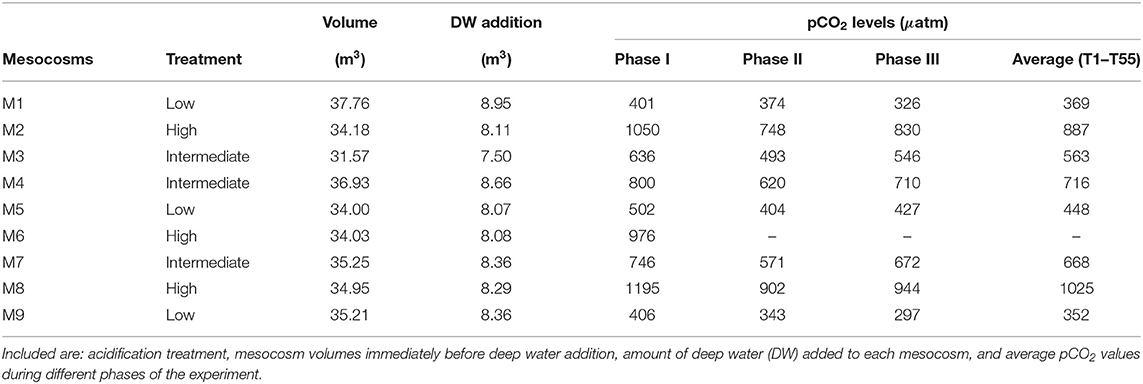
Table 2. Mesocosm experimental setup from Table 1 in Taucher et al. (2017).

The pCO₂ treatments were carried out by adding different amounts of CO₂-saturated seawater. During the addition, a special mixing device (“spider”) was constantly pulled up and down to ensure the homogeneous distribution of the CO₂-saturated seawater and to reach the desired pCO₂ levels (Riebesell et al., 2013). The initial CO₂ manipulation was carried out gradually in four steps over a period of 7 days, from T₀ to T₆, to avoid an abrupt disturbance. To correct the loss of CO₂ through air-sea exchange, two more pCO₂ additions were performed during the 55 days of the experiment: one at the end of phase II before the deep-water addition (on T₂₁), and one during phase III (on T₃₈) (Taucher et al., 2017). During the whole 55-days-long experiment the pCO₂ gradient among mesocosms was reasonably maintained (Figure 1). Table 2 summarizes the average pCO₂ levels in every mesocosm per phase of the experiment.

FIGURE 1

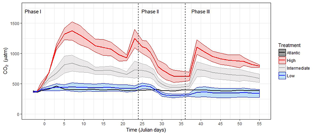
Figure 1. pCO₂ levels throughout the experiment, redrawn from Taucher et al. (2017). Note that, apart from the enrichment at the beginning of the experiment, two more enrichments were conducted on T₂₁ and T₃₈, ensuring that the gradient among the mesocosms was maintained during the whole experiment. Maximum and minimum values represent the Standard Deviation around the mean of pCO₂ in the mesocosms with the same treatment. We grouped the samples according to Algueró-Muñiz et al. (2019), blue = low-pCO₂ (M1, M5, and M9), gray = intermediate-pCO₂ (M3, M4, and M7), red = high-pCO₂ (M2 and M8). See Tables S19–S22.

After 24 days of oligotrophy (Phase I), an upwelling event was simulated by enriching nine mesocosms with nutrient-rich deep-water. Until T₂₃, the average concentration of the inorganic nutrients was very low. NO₃⁻+NO₂⁻, PO₄³⁻ and Si(OH)₄, were 0.06, 0.03, and 0.03 μmol L⁻¹, respectively (Figure 6 in Taucher et al., 2017). The pCO₂ levels in these mesocosms ranged from 400 to 1,200 μatm.

The upwelling event was simulated by replacing 20% of the mesocosms' volume by nutrient-rich deep-water with NO₃⁻+NO₂⁻, PO₄³⁻, and Si(OH)₄ concentrations of 16.50, 1.05, and 7.46 μmol L⁻¹, respectively (Figure 6 in Taucher et al., 2017). This replacement ensured an input of inorganic nutrients similar to those reported in this region's natural upwelling events (Taucher et al., 2017). To do that, around 85 m³ of nutrient-rich seawater was collected from a depth of 650 m by a “deep-water collection system” on T₂₂ (Taucher et al., 2017). The next day, T₂₃, defined amounts of water were carefully removed from the mesocosms at 5m depth. Then, during the night of the following day, T₂₄, an equal volume of nutrient-rich deep-water was added. This night-time addition was designed to minimize the phytoplankton nutrient uptake or growth during the nutrient-enrichment process. An injection device similar to the “spider” was used to ensure the desired mixing ratio of about 20% of the mesocosms' volume. Table 2 summarizes the total and deep-water volumes in every mesocosm. After the deep water addition, the final NO₃⁻+NO₂⁻, PO₄³⁻, and Si(OH)₄ concentrations in the mesocosms were 3.15, 0.17, and 1.60 μmol L⁻¹, respectively.

Subsequently, the phytoplankton community bloomed (Phase II) until nutrient depletion. Between T₂₈ and T₃₀, the inorganic nutrients dropped to values close to detection limit (Figure 6 in Taucher et al., 2017). At this point, the Post-bloom (Phase III) began. All the mesocosms showed similar trends in chlorophyll a (chl-a) and biomass during these three phases (Taucher et al., 2018).

Here, during the simulated deep-water upwelling event, we assessed how ocean acidification impacted the potential respiration, the phytoplankton biomass, and the proteinaceous biomass of the microplankton community in the 0.7–50.0 μm size-range. We then used these measurements, along with taxonomic observations, to parse out information on the anabolic and catabolic aspects of this community. The community was comprised of pico, nano, and microplankton parts but, from here on, we will call it “microplankton” to ease the discussion. The phytoplankton part of this community was dominated by cyanobacteria, but it also included diatoms, prymnesiophytes, chrysophytes, autotrophic nanoflagellates, and autotrophic dinoflagellates (Hernández-Hernández et al., 2018; Taucher et al., 2018). In addition, the micro-zooplankton part was dominated by aloricate ciliates and heterotrophic dinoflagellates (Algueró-Muñiz et al., 2019). During the simulation of the upwelling event, different stages of the phytoplankton bloom resulted in community composition shifts, ranging from an autotroph-dominated community to a heterotroph-dominated one (Hernández-Hernández et al., 2018; Taucher et al., 2018; Algueró-Muñiz et al., 2019). Here, we assessed how these changes in the microplankton community affected the ratio of the potential respiration of the entire microplankton community to the potential primary productivity of the phytoplankton. We used this information to evaluate how heterotrophic or autotrophic the community was, throughout the duration of the experiment.

A more detailed description of the study site, experimental design, key events, overall sampling, and measurements was reported in Taucher et al. (2017).

2.2. Sampling

Seawater for variables that are sensitive to gas exchange, such as dissolved inorganic carbon, inorganic nutrients or pH, was collected every 2 days during Phase I and III and every day during Phase II. The depth-integrated water-sampler (IWS, HYDRO-BIOS, Kiel) was used to take in a total volume of 5 L uniformly distributed over the mesocosms depth (0–13 m in every mesocosm, and in the surrounding Atlantic waters as a reference level for all the parameters that were measured in the Gran Canaria 2014 KOSMOS experiment). Additionally, an average total volume of 60–70 L per mesocosms was collected every sampling day using a custom-built pump-system. Chl-a and the phytoplankton community were measured in these samples.

The water column plankton community between 0.7 and 50.0 μm was sampled for potential respiration and biomass every 4 days during Phase I and III and every 2 days during Phase II. This collection frequency was lower than that for the other variables to avoid depleting the mesocosms' plankton community. During Phase II the collecting frequency was doubled in all the variables to properly monitor the changes in the plankton community during the phytoplankton bloom. This sample consisted of an aliquot (2–5 L) from the custom-built pump-sampling, per mesocosm. It was filtered through a 50 μm net before passing through a GF/F glass fiber filter (Whatman 0.7 μm nominal pore size) until the filter was clogged (always before 1h of filtration). The filters were frozen in liquid nitrogen and stored at −80°C until their treatment in the laboratory. All the samples were analyzed within 6 months after the experiment. The filters were homogenized at 0–4°C in 0.1M phosphate buffer, by a Teflon^® 2mL-pestle PYREX^® Potter-Elvehjem tissue grinder (homogenizer) at 2,600 rpm for 2 min. Crude homogenates were centrifuged (0–4°C) at 4,000 rpm (1,500 g) for 10 min.

2.3. Nutrients, Chlorophyll a (chl-a) and Water-Column Community Composition

The overall data related to the nutrient variability, chl-a, and the water-column community composition (both phytoplankton and microzooplankton) used in the interpretation and discussion of the results of this study were reported by Taucher et al. (2017), Hernández-Hernández et al. (2018), and Algueró-Muñiz et al. (2019).

Chl-a in the custom-built pump-sample was measured by HPLC (Barlow et al., 1997). Subsamples were homogenized in acetone 90% using glass beads in a cell mill. They were centrifuged at 5,200 rpm for 10 min at 4°C. The supernatant was filtered (0.2 μm PTFE filters, VWR International) and used to determine the phytoplankton pigment concentration in a Thermo Scientific HPLC Ultimate 3000 with an Eclipse XDB-C8 3.5 u 4.6 × 150 column. CHEMTAX software (Mackey et al., 1996) was used to classify phytoplankton on the basis of taxon-specific pigment ratios. Every 8 days, subsamples from the IWS were used to determine the microzooplankton abundances in order to be consistent with the mesozooplankton sampling. More frequent mesozooplankton sampling would, too rapidly, deplete the zooplankton community. Samples were immediately fixed with acidic Lugol (1–2%) solution and stored in the dark in 250 mL brown glass bottles. To identify and count the microzooplankton, the Utermöhl (1931) technique was applied using an inverted microscope (Axiovert 25, Carl Zeiss) (Algueró-Muñiz et al., 2019).

2.4. Potential Respiration

Potential respiration (Φ) was determined from ETS activity (Packard and Williams, 1981; Packard and Christensen, 2004) incorporating the modifications described in Kenner and Ahmed (1975) and Gómez et al. (1996). The original assay (Packard, 1971) is descended from a classical succinate-INT reductase assay (Nachlas et al., 1960) in which the maximum velocity is assured by saturating the reaction with the reactants. The ETS measurements were made on the centrifuged supernatant from the subsamples of custom-built pump-sample of the microplankton community (0.7–50.0 μm) (see section 2.2).

After centrifugation, we mixed 0.1 mL of the supernatant with the enzyme substrates (0.3 mL of a solution of 1.70 mM NADH and 0.25 mM NADPH prepared in the same buffer used during the homogenization of the sample) and with 0.1 mL of INT [2 mg INT mL⁻¹ in deionized H₂O] in a cuvette. The absorbance increase of the INT-formazan at 490 nm was continuously monitored spectrophotometrically at 18°C in 1cm path-length cuvettes for 8 min (Packard and Christensen, 2004), inside the Cary100 UV-Vis Spectrophotometer (Agilent Technologies). The regression line of absorption vs. time was used to calculate the ETS activity and potential respiration rates (Φ) after Packard and Christensen (2004). The tetrazolium salt, INT (p-Iodonitrotetrazolium Violet, Sigma #I8377) was reduced by the respiratory ETS enzymes, serving as the electron acceptor instead of O₂ (Lester and Smith, 1961; Smith and McFeters, 1997). INT accepts two electrons whereas O₂ would accept four. Thus, the INT-formazan production rate (δINT/δt) is stoichiometrically related by a factor of 2 to ETS activity (δe⁻/δt) and by a factor of 0.5 to Φ. In other words on a molar basis, δe⁻/δt = 2·δINT/δt and Φ = 0.5·δINT/δt where Φ is in units of μmol O₂, if INT is in μmol. Blanks were run without the ETS substrates in order to subtract the contribution of the background non-enzymatic and enzymatic reduction of the INT (Maldonado et al., 2012). Φ was reported in μmol O₂ min⁻¹ (mL of homogenate)⁻¹ units. To convert to μLO₂ h⁻¹ (mL of homogenate)⁻¹, multiply Φ by the volume occupied by one μmol of gas (22.4 μL μmol⁻¹) and by 60 min h⁻¹. Finally, to relate this Φ [in μL O₂ min⁻¹(mL of homogenate)⁻¹] to one L of the mesocosm water, we need to multiply it by the total volume of the homogenate of the sample and then, to divide it by the volume of sample that was filtered as stated in section 2.2 (an aliquot of 2–5 L from each mesocosm). Thus, after this operation, Φ is reported in μL O₂ h⁻¹ (L of seawater)⁻¹. All the Φ rates were corrected to in situ temperatures using the Arrhenius equation and an activation energy of 15 kcal mol⁻¹ (Packard et al., 1975).

2.5. The Φ/chl-a Ratio

Here, we calculated an index of the community potential respiration relative to the phytoplankton by dividing Φ (see section 2.4) by the chl-a concentrations (see section 2.3). This ratio (Φ/chl-a) was reported in μL O₂ h⁻¹ (μg chl-a)⁻¹ units. However, in the literature, Φ/chl-a, Φ or chl-a have been reported in other units. In order to facilitate comparison, in Table 1, we used conversion factors that were explained in the Supplementary Material. In addition, some of the Φ data used in Table 1 were originally measured by different versions of the ETS method. In order to facilitate comparison between the Φ data measured by different methods, Christensen and Packard (1979) assessed the relationship between them, and reported different conversion factors. These Φ data are comparable now after using these conversion factors (Christensen and Packard, 1979) (see Supplementary Material). In Table 1 we used ETS and chl-a data from both old and new papers, before and after the development of the kinetic ETS assay of Packard and Christensen (2004). Without this understanding and exercise one cannot compare ETS data from this millennia with ETS data from the previous millennia.

2.6. Particulate Protein and Its Variability

We measured biomass (B) spectrophotometrically as particulate protein on the same homogenates used for the enzyme activity assays. We followed the protein method of Lowry et al. (1951) as modified by Rutter (1967) and Mart́ınez et al. (2020) with bovine serum albumin (BSA) as the standard for calibration. This method consisted of a chemical reaction, where 200 μL of the supernatant of the centrifuged homogenate (see section 2.2): (1) was mixed with 1 mL of the “Rutter” solution (110 mL of a solution of 0.19 M Na₂CO₃, 0.10 M NaOH, and 0.71 mM Na-K tartrate, mixed with 2.2 mL of a solution of 0.02 M CuSO₄·5H₂O) in a cuvette stored in ice; (2) then mixed, after 10 min, with 100 μL of Folin's reagent (C₁₀H₅NaO₅S, diluted 1:1 in doubled-distilled H₂O) at laboratory temperature (22°C); and (3) after being stored in darkness for 40 min at 22°C, was pipetted into 1 cm path-length cuvette, inside the Cary100 UV-Vis Spectrophotometer (Agilent Technologies) to measure the absorbance at 750 nm. B was reported as mg protein (L of seawater)⁻¹.

The change in particulate protein per day (P_N) was determined by calculating the first derivative (differential analysis) of the B time-course (Figure 2). Thus, P_N = δB/δt (Figure 2, bottom panel). Positive values reflected net protein formation in which protein synthesis exceeded “losses” caused by remineralization, grazing, and sinking. Negative PN indicated a net protein loss. Note that if both primary and secondary productivity (PP and SP) data had been available, we could have combined these measurements (in terms of mg C L⁻¹d⁻¹) in order to calculate the biomass loss (BL) in the system (P_N = PP + SP − BL). Even though PP was addressed by Hernández-Hernández et al. (2018) in this KOSMOS study, there were no SP data, so the BL could not be calculated. However, differential analysis calculates when BL >(PP + SP) and the reverse, by transforming a concentration time-course into a rate-of-change time-course. This generates maxima (peaks) and minima (troughs) in the time-courses of dB/dt that identify when B was increasing and disappearing fastest.

FIGURE 2

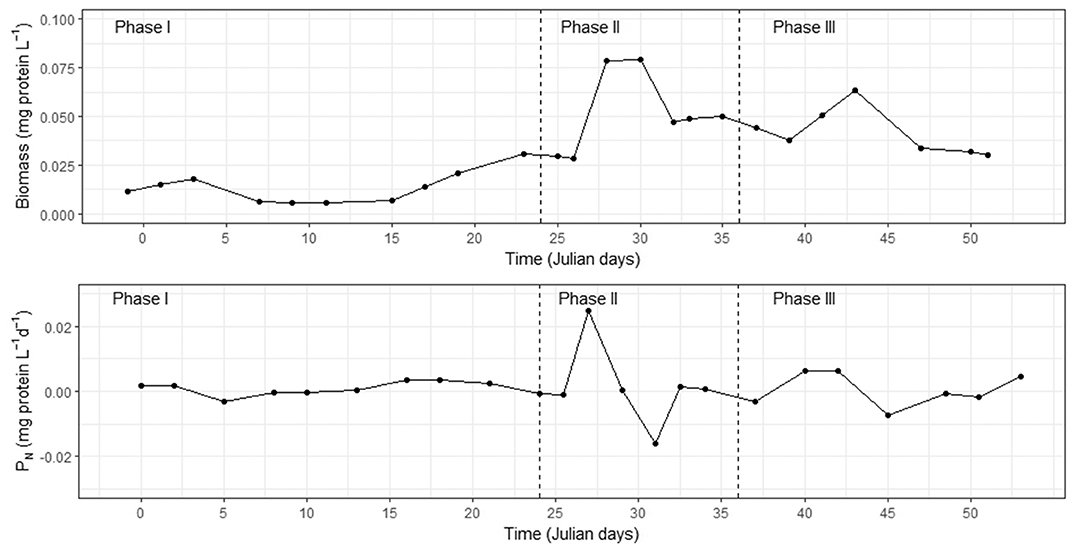
Figure 2. (Top) Time-course of particulate protein (B) in M1 during the three phases of the entire 55 days experiment. (Bottom) Illustrative example of differential analysis for B in M1. The curves show the first derivative (dB/dt). This calculation converts the static property, B, into a time-dependent property, the change in particulate protein per day (P_N). As mentioned in section 2.6, P_N is a dynamic property, a measure of net microplankton biomass growth, when positive, and a measure of net microplankton biomass decline when negative. P_N oscillates aperiodically between these two stages.

2.7. Data Analysis and Statistics

The Mann-Whitney test was used to compare Φ, B and chl-a distributions between the different pCO₂ levels in the different mesocosms (Hollander et al., 2013) (see Tables S16–S18). In addition, the integrative analysis was applied to the area below the data curves (Figure 2, top panel) by the trapezoidal approximation method using the trapz function of the pracma R-Cran package (Borchers, 2017). The Mann-Whitney test analysis of the static Φ, chl-a, and B time-courses did not show significant differences, but because integration amplified the time-course signals, new statistical analysis of the integral in relation to increasing pCO₂ levels, did show significant differences.

The integral of Φ, chl-a, and B by each phase, in each mesocosm, was normalized by the number of days of the phases (Phase I: 24 days, Phase II: 11 days, Phase III: 20 days), in order to facilitate the comparison not only between different pCO₂ levels, but also between phases (Equations 1–3).

$\begin{array}{ll}\text{Normalized integral of}\Phi ={\displaystyle {\int }_{t1}^{t2}}\Phi (t)dt/\Delta t& (1)\end{array}$

$\begin{array}{ll}\text{Normalized integral of chl-}a={\displaystyle {\int }_{t1}^{t2}}\text{chl-}a(t)dt/\Delta t& (2)\end{array}$

$\begin{array}{ll}\text{Normalized integral of B}={\displaystyle {\int }_{t1}^{t2}}B(t)dt/\Delta t& (3)\end{array}$

where t₁ and t₂ are the initial and final days of each phase, respectively, and Δt is the number of days in each phase. Then, the integrals were plotted against the average-pCO₂ level of each mesocosm during the related phase (x-axis in Figure 3). The relationship between the integrative analysis of Φ, chl-a, and B and the increasing pCO₂ levels was addressed by linear regression, considering both the slope (α) and the goodness of fit (R² for linear regression) (Tables S13–S15) (Figure 3). Note that α is expressed in the units related to the relationship between two parameters. When we are studying the relationship between B and pCO₂, α is reported in mg proteins L⁻¹ (μatm CO₂)⁻¹. As this integrative analysis was normalized by the number of days in every phase to allow comparison among phases, the α was finally reported in mg proteins L⁻¹ (μatm CO₂)⁻¹ (phase-day)⁻¹ units. Accordingly, in analysing the relationship between chl-a and pCO₂, α was reported in mg chl-a L⁻¹ (μatm CO₂)⁻¹ (phase-day)⁻¹ units. Also, in analysing the relationship between Φ and pCO₂, α was reported in μL O₂ h⁻¹ L⁻¹ (μatm CO₂)⁻¹ (phase-day)⁻¹ units.

FIGURE 3

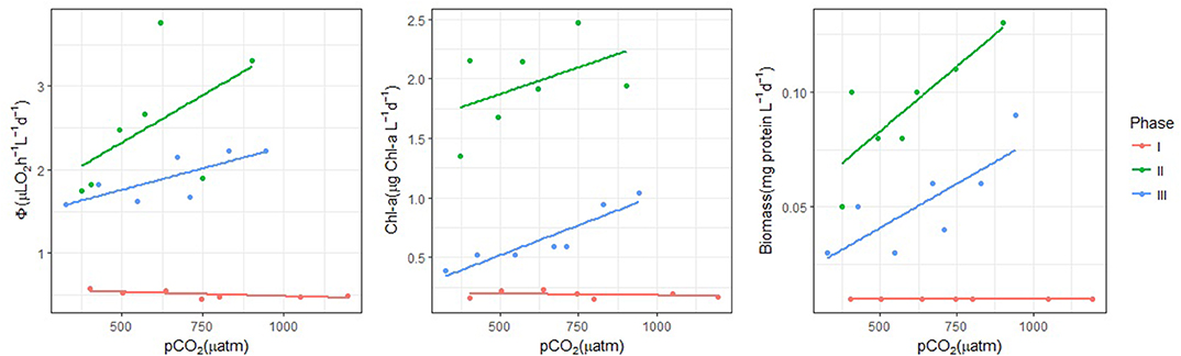
Figure 3. Integral analysis of potential respiration, chl-a and biomass by experiment phase and treatment. M9 values have been removed. Note that every point represents the integral of each parameter normalized by the number of days in every phase (d) (Phase I: 24 days, Phase II: 11 days, Phase III: 20 days). These integral values are plotted against the CO₂-level. Observe that the red color represents Phase I; green represents Phase II; and blue represents Phase III. See Tables S13–S15.

On a separate issue, note that the communities in M2 and M8, the most acidified mesocosms, began to clearly differ from the other mesocosms at the end of Phase II. That was when a harmful algal species (HAS) bloomed and disrupted the community. As the trends of the vital parameters may vary depending on whether or not M2 and M8 were considered in the analysis, we addressed both scenarios when we assessed α and R² in Phase II and Phase III.

3. Results

3.1. Phase I: Responses to CO₂-Treatments Under Low-Nutrient Conditions

During this oligotrophic phase, all the mesocosms followed the same trend (Figure 4) (Taucher et al., 2017, 2018). The 0.7–50.0 μm-sized microzooplankton community comprised 13 different taxonomic groups of heterotrophic dinoflagellates and ciliates (Algueró-Muñiz et al., 2019). During this phase the microzooplankton abundance was 4.30 ± 2.07·10³ individuals L⁻¹ in the low-pCO₂ mesocosms, 3.31 ± 1.48·10³ individuals L⁻¹ in the intermediate-pCO₂ mesocosms and 4.20 ± 1.13·10³ individuals L⁻¹ in the high-pCO₂ mesocosms (see Tables S31–S33, respectively; Algueró-Muñiz et al., 2019). In addition, the picocyanobacteria Synechococcus constituted 70–80% of total chl-a in the mesocosms. Here, the phytoplankton community evolved differently from the Atlantic-surrounding-water community, which was dominated by cyanobacteria. In all mesocosms, from T₁₅ onwards, the former cyanobacteria-dominated community evolved to a mixed one: diatoms, prymnesiophytes, chrysophytes and cyanobacteria (Hernández-Hernández et al., 2018; Taucher et al., 2018).

FIGURE 4

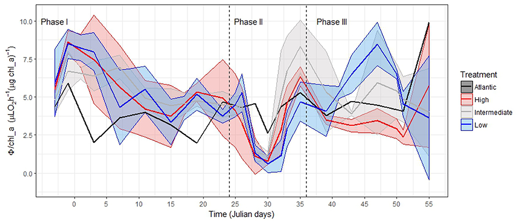
Figure 4. Potential respiration per chl-a during Phase I: Oligotrophic phase; Phase II: Bloom phase after deep-water addition; and Phase III: Post-bloom phase after nutrient-depletion. Maximum and minimum values represent the Standard Deviation around the mean of Φ/chl-a in the mesocosms with the same treatment (see Table 2). We grouped the samples according to Algueró-Muñiz et al. (2019), blue = low-pCO₂ (M1, M5, and M9), gray = intermediate-pCO₂ (M3, M4, and M7), red = high-pCO₂ (M2 and M8). See Tables S23–S26.

The Φ/chl-a ratio shifted down from 8.0 at T₀ to 3.4 μL O₂ h⁻¹ (μg chl-a)⁻¹ at T₂₃ (Figure 4). During this phase, the average Φ/chl-a ratios in the high-pCO₂ mesocosms (M2 and M8), in the intermediate-pCO₂ mesocosms (M3, M4, and M7) and in the low-pCO₂ mesocosms (M1, M5, and M9) were 5.7 ± 1.6, 5.5 ± 1.0, and 5.6 ± 1.8 μL O₂ h⁻¹ (μg chl-a)⁻¹, respectively. In the Atlantic samples during this time, Φ/chl-a shifted down from 4.7 to 2.0 μL O₂ h⁻¹ (μg chl-a)⁻¹, resulting in an average Φ/chl-a ratio of 3.7 ± 1.3 μL O₂ h⁻¹ (μg chl-a)⁻¹ (Figure 4).

Throughout the entire phase, P_N was undetectable (0.000 ± 0.002 mg proteins L⁻¹ d⁻¹, from T₀ to T₂₁) until it increased in the last 2 days (Figure 5). This indicated, for the first 21 days, a steady state where both biomass-production and biomass-loses were balanced. Then, at T₂₂ through T₂₄, P_N shifted up (Figure 5) to 0.006 ± 0.005 mg proteins L⁻¹ d⁻¹ at T₂₄. This P_N rise coincided and seemed stimulated by a natural nutrient addition from a Sahara-dust deposit event (“Calima”). The total dry-deposition flux was similar to other weak dust events (Gelado-Caballero et al., 2012; Taucher et al., 2017). However, in our KOSMOS experiment, this dust-deposition event was not considered to significantly affect the growth of the phytoplankton community because this growth was occurring before the “Calima” event (Taucher et al., 2017).

FIGURE 5

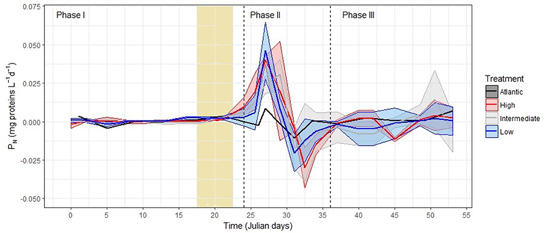
Figure 5. P_N of the microplankton community, as the first derivative of biomass, during Phase I: Oligotrophic phase; Phase II: Bloom phase after deep-water addition; and Phase III: Post-bloom phase after nutrient-depletion. The vertical light-yellow column on the left represents the dust-deposition event (“Calima”) that occurred from T₁₆ to T₂₂. Note that negative values reflects the net loss of biomass, when the combination of sinking, remineralization, grazing and other losses outweighs the biomass production by both autotrophs and heterotrophs. Maximum and minimum values represent the Standard Deviation around the mean of P_N in the mesocosms with the same treatment (see Table 2). We grouped the samples according to Algueró-Muñiz et al. (2019), blue = low-pCO₂ (M1, M5, and M9), gray = intermediate-pCO₂ (M3, M4, and M7), red = high-pCO₂ (M2 and M8). See Tables S27–S30.

Regarding the effects of increasing pCO₂ on Φ, chl-a and B, application of the Mann-Whitney test to the entire 55-days experiment did not show significant differences (p < 0.05) that could be clearly related to these treatments. However, it did reflect significant differences between the surrounding Atlantic waters and the mesocosms during the entire experiment (Tables S16–S18). In addition, after inspecting the data-curves at different pCO₂ levels (Figure 2), we anticipated trends in the biological parameters to differ both between mesocosms and within the three different phases of the experiment. However, the trend-differences were low, so to amplify the signals associated with the increasing pCO₂, we integrated the biological data for Φ, chl-a and B over each phase and each mesocosm, and then, normalized them by the numbers of days in each Phase (Phase I: 24 days, Phase II: 11 days, Phase III: 20 days). We then plotted these integrals against pCO₂ (Figure 3). The results showed that during Phase I, the integrals of Φ, chl-a and B were consistently the lowest values calculated (0.49 ± 0.06 μL O₂ h⁻¹ L⁻¹ d⁻¹, 0.19 ± 0.03 mg chl-a L⁻¹ d⁻¹, and 0.01 ± 0.00 mg protein L⁻¹ d⁻¹, respectively, Figure 3, Table 3, Tables S13–S15). Considering this, we concluded that no pCO₂-related effects occurred during this phase.

TABLE 3

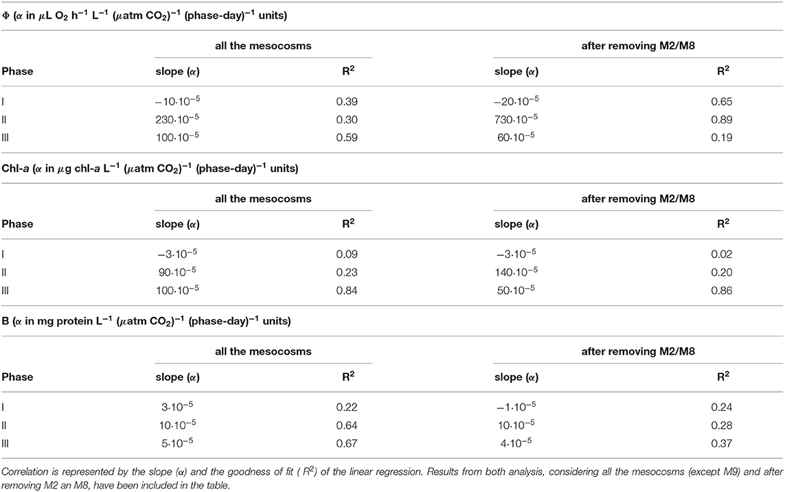
Table 3. Correlation between the integrative analysis of the vital parameters (Φ, chl-a, and B), normalized per phase and mesocosm, and the pCO₂ levels.

3.2. Phase II: Responses During the Deep-Water Addition Event

The deep-water addition on T₂₄ resulted in a phytoplankton bloom between T₂₈ and T₃₀ in all the mesocosms (Taucher et al., 2017, 2018; Hernández-Hernández et al., 2018). Here, the diatoms constituted up to 80% of total biomass (see Figure 2 in Taucher et al., 2018). During this bloom, the average Φ/chl-a ratio dropped to the lowest value in the whole experiment [1.1 ± 0.6 μL O₂ h⁻¹ (μg chl-a)⁻¹ at T₃₀] and was essentially the same for the high, medium, and low pCO₂ mesocosms. It varied only from 0.6 to 1.2 μL O₂ h⁻¹ (μg chl-a)⁻¹ among them (Figure 4). Following this bloom, on T₃₃, the microzooplankton abundances increased in the low- and intermediate-pCO₂ mesocosms (16.83 ± 12.99·10³ and 23.36 ± 12.41·10³ individuals L⁻¹, respectively, see Tables S31–S33) (Algueró-Muñiz et al., 2019). This increase was driven mainly by the proliferation of dinoflagellates (further information regarding individual taxa in Algueró-Muñiz et al., 2019). However, the microzooplankton community remained low in the high-pCO₂ mesocosms (680 ± 80 individuals L⁻¹, Table S33). At this moment, a harmful algal species (HAS), Vicicitus globosus, proliferated in the high-pCO₂ mesocosms (Riebesell et al., 2018).

During the bloom, P_N peaked between 1 and 2 days before the chl-a maximum in all the mesocosms (0.039 ± 0.013 mg proteins L⁻¹d⁻¹) (Figure 5). This proteinaceous biomass increase suggested that PP and SP clearly overcame BL. In contrast, during the 24 h after the peak (Figure 5), the combination of remineralization, grazing, sinking, and other losses resulted in a net-decrease in B of −0.023 ± 0.008 mg proteins L⁻¹d⁻¹. The average P_N in all the mesocosms was 0.005 ± 0.024 mg proteins L⁻¹d⁻¹.

Even though all the mesocosms behaved in a similar way during the bloom, afterwards, until nutrient depletion, the plankton communities evolved differently. Integrals of chl-a revealed a positive trend in the pCO₂ effects (α = 90·10⁻⁵). Note that, in the analysis, the units of the slope (α) differ depending on the parameter (see Table 3). However, the goodness of fit, between chl-a and pCO₂, was weak (R² = 0.23, Table 3). Furthermore, this trend depended strongly on M2 and M8. The communities in M2 and M8, the most acidified mesocosms, began to clearly differ from the other mesocosms at the end of Phase II. That was when V. globosus bloomed and disrupted the community. Because of this, the trends of the vital parameters varied depending on whether or not M2 and M8 were considered in the analysis. In the case of chl-a, after removing M2 and M8, the goodness of fit of the positive trend in Phase II was weaker (R² = 0.20, Table 3, Table S14). Similarly, the integral analysis of B in Phase II, showed a slight positive effect (α = 10·10⁻⁵), and this relationship was even weaker after removing M2 and M8 data (Figure 3, Table 3, Table S15). On the contrary, the relationship between Φ and pCO₂ was found to be clearly positive during this phase (α = 230·10⁻⁵), being particularly strong after removing the M2 and M8 data (α = 730·10⁻⁵, Table 3, Figure 3, Table S13).

When comparing the normalized integral values of all these vital parameters between phases, we found that the highest values occurred during Phase II (Figure 3), due to the phytoplankton bloom (2.39 ± 0.81 μL O₂ h⁻¹ L⁻¹ d⁻¹ in the case of Φ, 2.06 ± 0.46 mg chl-a L⁻¹ d⁻¹ in the case of chl-a, and 0.10 ± 0.24 mg protein L⁻¹ d⁻¹ in the case of B). The increase in the normalized integral, from Phase I to Phase II, illustrated the positive effect of the addition of nutrient-enriched deep water in boosting the microplankton community. Note that not only did this positively impact chl-a, but it also positively impacted Φ, potential respiration.

3.3. Phase III: Responses to the CO₂-Treatments During the Nutrient Depletion Phase

After the nutrient depletion, the communities differed among the treatments. Generally speaking, the biomass of phytoplankton groups dropped during the nutrient depletion that followed the diatom bloom around T₃₇ (see Figure 2 in Taucher et al., 2018). However, increasing pCO₂ levels led to additional differences. During the post-bloom phase, the diatom biomass in high-pCO₂ mesocosms was about 2-fold higher than in low-pCO₂ mesocosms (Taucher et al., 2018). This was driven by the dominance of Guinardia striata (for further information of individual taxa see Taucher et al. (2018)). In addition, V. globosus proliferated in the high-pCO₂ mesocosms until T₄₇ (Riebesell et al., 2018). Then, when V. globosus began to decline, the microzooplankton abundance rose, reaching a maximum of 24.91 ± 7.68 · 10³ individuals L⁻¹ in the high-pCO₂ mesocoms on T₅₀ (Table S33). Unlike the low- and intermediate-pCO₂ mesocosms, this increase in microzooplankton was clearly driven by ciliates instead of heterotrophic dinoflagellates (see further information about individual taxa in Algueró-Muñiz et al., 2019). In the low- and intermediate-pCO₂ mesocosms, while the phytoplankton biomass dropped, the microzooplankton abundances were high until the end of the experiment (20.49 ± 15.13·10³ and 14.22 ± 8.24·10³ individuals L⁻¹, respectively; Tables S31, S32). The microzooplankton abundance peaked between T₃₃ and T₄₁ in the intermediate-pCO₂ mesocosms (21.43 ± 9.84·10³ individuals L⁻¹) whereas, in the low-pCO₂ mesocosms, the microzooplankton reached the maximum abundance between T₄₁ and T₅₀ (20.49 ± 15.13 · 10³ individuals L⁻¹) (Algueró-Muñiz et al., 2019).

The Φ/chl-a peaked when the microzooplankton, dominated by heterotrophic dinoflagellates, peaked in both low pCO₂ (M1, M5, and M9, between T₄₃ and T₄₇) and intermediate pCO₂ mesocosms (M3 and M4 between T₃₂ and T₃₅, and M7 between T₃₅ and T₃₉) (Figure 4; Algueró-Muñiz et al., 2019). Here, Φ/chl-a ratios rose sharply up to 10.0 μL O₂ h⁻¹ (μg chl-a)⁻¹ (7.5 ± 1.6 and 7.6 ± 1.5 μL O₂ h⁻¹ (μg chl-a)⁻¹ in the low-pCO₂ mesocosms and in the intermediate-pCO₂ mesocosms, respectively, during the microzooplankton peak). However, in high pCO₂ mesocosms (M2 and M8), where V. globosus bloomed, the Φ/chl-a ratio remained between 2.5 and 7.0 μL O₂ h⁻¹ (μg chl-a)⁻¹ (4.1 ± 1.5 μL O₂ h⁻¹ (μg chl-a)⁻¹). Note that these values were measured from T₃₅, the nutrient depletion (Taucher et al., 2017), to T₄₇, when the V. globosus community declined (Riebesell et al., 2018).

Finally, considering all the integrals of B in the mesocosms, we saw a positive relationship between B and pCO₂ (α = 5·10⁻⁵, R² = 0.67, Figure 3, Table 3). However, this relationship depended strongly on M2 and M8. If we removed M2 and M8, this relationship was weaker in both the slope and the goodness of fit (α = 4·10⁻⁵, R² = 0.37, Table 3, Table S15). Considering Φ during Phase III, we found that the pCO₂ effects on the potential respiration were slightly positive (α = 100·10⁻⁵, R² = 0.59). This relationship was even weaker after removing M2 and M8 data (α = 60·10⁻⁵, R² = 0.19, Table 3, Table S13). With the chl-a integrals, we again saw a positive relationship with pCO₂ during this phase (α = 100·10⁻⁵, R² = 0.84, Table 3, Figure 3, Table S14). As with the integrals of B, this positive pCO₂ effect on chl-a was smaller after removing M2 and M8 data (α = 50·10⁻⁵, R² = 0.86, Table 3, Table S14). All in all, the normalized integral analysis in Phase III, considering all the mesocosms, yielded lower values than in Phase II, but they were still higher than those in Phase I. This suggested that the positive effects of the bloom on the community remained for a while after nutrient depletion.

During the post-bloom phase (III), the observed changes in the community composition did not impact P_N. Although it was more variable than in Phase I, P_N trends were to stay close to zero in all the mesocosms (−0.0009 ± 0.009 mg proteins L⁻¹d⁻¹, Figure 5). This suggested that, after the bloom and the nutrient depletion, the community began to approach a steady state close to the one in Phase I.

4. Discussion

4.1. Using the Φ/chl-a Ratio to Detect Metabolic Shifts in Microplankton

In this paper, Φ includes the potential catabolic respiratory activity of all the organisms in the 0.7–50.0 μm sized community of the sample. Chl-a, a proxy for phytoplankton biomass, is also considered here as an index of potential phytoplankton anabolic activity, i.e., potential primary productivity. Accordingly, as a hypothesis, we interpret the ratio, Φ/chl-a, as an index of potential catabolism to potential phytoplankton anabolism. On the basis of observations, we hypothesize that this ratio will be low (around 1) when the phytoplankton, as photoautotrophs, dominate the microplankton community and high (around 10) when heterotrophs dominate it. From this KOSMOS experiment and from the literature, we observed Φ/chl-a to vary from 0.2 to 2.3 in areas of photoautotrophic dominance to 7.6–28.4 in areas of heterotrophic dominance (Table 1). Throughout our 55-days experiment, the reference Φ/chl-a ratio from the microplankton community in the mixed Atlantic waters outside the mesocosms varied around 4.3 ± 1.7 μL O₂ h⁻¹ (μg chl-a)⁻¹, an intermediate value. This microplankton community was composed of Prochlorococcus and Synechococcus-type cyanobacteria, picoeukaryotes, nanoeukaryotes, diatoms (Hernández-Hernández et al., 2018; Taucher et al., 2018), ciliates (aloricate and loricate), and both autotrophic and heterotrophic dinoflagellates (athecate and thecate) (Algueró-Muñiz et al., 2019).

However, from the very beginning of the experiment, the Φ/chl-a ratio was higher in the nine mesocosms [5.6 ± 2 μL O₂ h⁻¹ (μg chl-a)⁻¹] than in the ambient Atlantic waters. The phytoplankton community evolved, in all mesocosms, from a cyanobacteria-dominated community to a mixed one: diatoms, prymnesiophytes, chrysophytes and cyanobacteria (Hernández-Hernández et al., 2018). In addition, these authors found that the nanoplankton dominated the biomass (50%) but not the chl-a (30%). This indicates that there was a mixed nanoplankton community of autotrophs and heterotrophs within the mesocosms, where the heterotroph contribution to potential respiration and to biomass was higher than in the surrounding Atlantic waters. On the other hand, the microzooplankton community (mainly aloricate ciliates and heterotrophic dinoflagellates) remained at low concentrations (Algueró-Muñiz et al., 2019). Thus, the mesocosm-enhancement effect on the Φ/chl-a ratio was mainly related to the shift in the nanoplankton toward a more heterotrophic community in which the potential respiration was augmented, but not the chl-a. All these Φ/chl-a results were consistent with those obtained from the Φ and chl-a measurements made in upwelled waters and in the euphotic zone in similar environments (Packard et al., 1974; Packard, 1979; Aŕıstegui and Montero, 1995) (see Table 1).

During Phase II, the Φ/chl-a ratio dropped to values lower than 1.7 μL O₂ h⁻¹ (μg chl-a)⁻¹ in all mesocosms. The mean value was 1.1 ± 0.6 μL O₂ h⁻¹ (μg chl-a)⁻¹ (Table 1), reflecting the shift in the community composition toward a phytoplankton bloom between T₂₈ and T₃₀(Taucher et al., 2017). These results were consistent with those reported at the chl-a maximum (Martinez et al., 1990; Martinez, 1991), in upwelled waters, and in the euphotic zone in similar environments (Aŕıstegui and Montero, 1995). They were slightly higher than those for the euphotic-zone community in eutrophic waters (Bangqin et al., 2005). They were also similar to those from different bloom conditions in the phytoplankton community (Packard et al., 2000) (see Table 1). From this evidence, we surmise that Φ/chl-a ratios lower than 2.5 μL O₂ h⁻¹ (μg chl-a)⁻¹ reflect, mainly, a photoautotrophic community (Table 1).

During the nutrient depletion and the post-bloom phase (III), there was large variability in the plankton community development and in the evolution of the Φ/chl-a ratio of the mesocosms (Figure 4). However, similar Φ/chl-a ratios were found in those mesocosms where the microzooplankton bloomed (M3, M4, M7, of the intermediate-pCO₂ mesocosms; and M1, M5, and M9, of the low-pCO₂ mesocosms) (Figure 4). First, the microzooplankton, dominated by small thecate and large athecate heterotrophic dinoflagellates (Algueró-Muñiz et al., 2019), bloomed in the intermediate mesocosms at the end of Phase II (T₃₂ and T₃₅ in M3 and M4, and during T₃₅ and T₃₇ in M7), when values of 7.6 ± 1.5 μL O₂ h⁻¹ (μg chl-a)⁻¹ were attained. This heterotrophic dinoflagellate community also bloomed in the weakly acidified mesocosms during Phase III (T₄₃ and T₄₇ in M1, M5, and M9), resulting in high Φ/chl-a ratios [7.5 ± 1.6 μL O₂ h⁻¹ (μg chl-a)⁻¹]. These high values are consistent to others reported from the euphotic zone in the Canary Islands (Aŕıstegui and Montero, 1995). In addition, even higher values were found in eutrophic waters when samples included mesozooplankton (Packard and Williams, 1981). From these records, we consider that Φ/chl-a ratios higher than 7.0 μL O₂ h⁻¹ (μg chl-a)⁻¹ reflect dominance of a heterotrophic microplankton community.

Lower Φ/chl-a of 4.1 ± 1.5 μL O₂ h⁻¹ (μg chl-a)⁻¹ characterized high-pCO₂ mesocoms (M2 and M8) at the end of Phase II and during the main part of Phase III. During those times, high pCO₂ levels stimulated V. globosus (Riebesell et al., 2018; Taucher et al., 2018). This HAS had a significantly negative effect on the micro- and mesozooplankton populations. Both dropped to the lowest values observed during the entire experiment (Riebesell et al., 2018; Algueró-Muñiz et al., 2019). On the other hand, diatoms persisted longer, probably due to weak grazing (Taucher et al., 2018). However, although these values were lower than those in heterotroph-dominated communities, they were not as low as expected for a photoautotroph-dominated one (<1.7 μL O₂ h⁻¹ (μg chl-a)⁻¹ as in Phase II). Indeed, even though the microzooplankton did not proliferate in M2 and M8 due to the presence of V. globosus, Φ in M2 and M8 reached high values as seen when microzooplankton bloomed in M3, M4, and M7 (5.3 ± 0.7 and 4.7 ± 1.1 μL O₂ h⁻¹ L⁻¹, respectively; Table S5). As a result, Φ/chl-a in M2 and M8 reached intermediate values [4.1 ± 1.5 μL O₂ h⁻¹ (μg chl-a)⁻¹], close to those from the Atlantic-water mixed community [4.3 ± 1.7 μL O₂ h⁻¹ (μg chl-a)⁻¹], and to those from the Phase I community in all mesocosms [3.4–8.0 μL O₂ h⁻¹(μg chl-a)⁻¹]. Φ/chl-a did not fall to the level of photoautotroph dominance [<1.7 μL O₂ h⁻¹ (μg chl-a)⁻¹]. Finally, at termination, when V. globosus became rare, aloricate ciliates bloomed in M2 and Φ/chl-a soared to 8.6 μL O₂ h⁻¹ (μg chl-a)⁻¹, indicating heterotrophic dominance.

All these values are consistent with the thinking of Martinez et al. (1990) and Martinez (1991), who found that the Φ/chl-a ratio was low in phytoplankton-dominated zones (such as upwelling systems, ocean fronts or chl-a maximum layers), and increased outside these areas, where the microheterotroph's contribution to the microplankton was higher. Here, in the KOSMOS experiment, thanks to the monitoring of the plankton-community's composition related to these values, we were able to observe the different characteristics of this composition throughout the observed Φ/chl-a range [0.6–10.0 μL O₂ h⁻¹ (μg chl-a)⁻¹] (see Table 1).

4.2. Acidification, Mixotrophy, and the Development of Vicicitus globosus

We ponder the reasons for the proliferation of V. globosus after nutrient depletion in the high pCO₂ mesocosms of M2 and M8 where it had higher Φ/chl-a ratios [4.1 ± 1.5 μL O₂ h⁻¹ (μg chl-a)⁻¹] than expected from reports of its being a pure autotroph (Chang, 2015). These higher ratios suggested both, that V. globosus had heterotrophic properties and that it could be mixotrophic. Mixotrophy is a major mode of nutrition among HAS (Burkholder et al., 2008). We noted that V. globosus was able to maintain its population during nutrient depletion (Riebesell et al., 2018). We know that V. globosus lacks pyrenoids (Chang et al., 2012), the organelle that optimizes CO₂ fixation by concentrating CO₂ in the chloroplast (Badger et al., 1998). From this, we deduce that V. globosus has an inefficient photosynthetic system under ambient pCO₂, but would be more efficient if pCO₂ were more concentrated. In this case, it would be able to compete favorably with other phytoplankton species. We know also, that V. globosus is a shape-shifter, able to change from a flagellated-shape to an amoeboid-shape and back in minutes (Chang et al., 2012). This ability, if accompanied by phagocytosis, would enable V. globosus to supplement its photosynthesis by using bacterivory. Furthermore, by killing both diatoms and microzooplankton and releasing their organic matter to the seawater (Chang, 2015), V. globosus would stimulate bacterial growth. It could then supplement its nutrition not only by feeding on bacteria, but also by ingesting the newly released organic matter. We realize this is hypothesis, but there is enough evidence and supporting logic behind it to encourage other research groups to test it in cultures of V. globosus.

4.3. The Use of Time-Courses of Static Variables to Calculate Dynamic Variables

To strengthen our analysis of the KOSMOS time-courses, we calculated the first-derivative (dB/dt) of the living biomass per time (P_N) (Figure 5). This derivative advanced the quantification and monitoring of the plankton time-dependent dynamics by converting time-course data on a “static” property, i.e., biomass or protein, into a dynamic one. Static properties lack a time dimension, dynamic properties have one. Here, when dB/dt is positive it reflects a net particulate protein production; if dB/dt is negative, it reflects a net loss of particulate protein. Both are designated, P_N. This type of derivative analysis is useful when direct rate measurements are not available. Using this technique, within the development of the phytoplankton bloom, four different stages were identified (Figure 5): a steady-state during Phase I; a net production of particulate protein after the deep-water addition; a net loss after the phytoplankton bloom; and an approach to a new steady-state after nutrient depletion.

4.4. Analysing the pCO₂ Effects on the Vital Parameters

Under the oligotrophic conditions of Phase I, no effects of the increasing pCO₂ levels were revealed in the integrative analysis of any of the vital parameters (Φ, chl-a, and B) (Figure 3). However, during Phase II, the communities in each mesocosm began to differ and these differences were greater at the end of Phase II in the highest pCO₂ mesocosms (Figure 3) where V. globosus began to bloom and impede microzooplankton growth. This population shift had a direct effect on Φ (Table 3). Considering the results of the integrative analysis of the community Φ, in absence of HAS, we found the increasing pCO₂ increased Φ. However, the proliferation of HAS at the end of Phase II, weakened this positive trend. This change reflected the lethal impact of V. globosus on the microzooplankton community, and consequently, on the catabolism in the whole community (Table S13). Increasing-pCO₂ levels seemed to stimulate B in the same way as they stimulated Φ during Phase II (Table 3). However, in the case of B, the R² was too weak to consider the trend significant. Regarding chl-a, increasing-pCO₂ levels seemed to increase it during the phytoplankton bloom and this effect was strengthened by the HAS proliferation, when M2 and M8 were considered in the analysis. These effects were likely related to a lack of grazing, as microzooplankton became scarce in these mesocosms. However, as in the case of B, the R² for the relationship between chl-a and pCO₂ was weak during this phase, so we cannot consider this a significant positive trend (Table 3).

In contrast, during Phase III, when V. globosus bloomed and the microzooplankton dropped to a minimum in the highest-pCO₂ mesocosms, the increasing pCO₂ levels led to higher chl-a values. Apart from the reduction of grazing on the phytoplankton community due to the presence of V. globosus, we suggest that V. globosus' photosynthetic system, whose lack of pyrenoids made it inefficient in low pCO₂ environments (Badger et al., 1998), was stimulated in the high pCO₂ mesocosms, leading to acidification's positive impact on chl-a. However, once the data from M2 and M8 were removed, this positive pCO₂ effect on chl-a was smaller (Table S14). This indicates that, even though increasing pCO₂ had a positive impact on the photoautotrophs in this study, the most important effect was linked to the presence of HAS, which impeded the zooplankton proliferation and the grazing on the phytoplankton community.

Finally, even though chl-a was stimulated, neither Φ nor B were significantly impacted by the increasing pCO₂ during Phase III. However, even though the goodness of fit was weak, the integrative analysis showed a slightly positive relationship. Considering the toxic effects of V. globosus on microzooplankton we would have expected a negative result. This positive trend, taking into consideration that microzooplankton were absent, leads to the hypothesis that V. globosus has a stronger catabolic pathway than common photoautotrophs.

5. Conclusion

The ratio, Φ/chl-a shifted up from a low of <1.7 μL O₂ h⁻¹ (μg chl-a)⁻¹ during the phytoplankton bloom, through intermediate ratios around 4.3 μL O₂ h⁻¹ (μg chl-a)⁻¹ for an autotrophic-heterotrophic community, and finally to high ratios of 10 μL O₂ h⁻¹ (μg chl-a)⁻¹ in a heterotrophic dinoflagellate community (Figure 4). We hypothesize that the Φ/chl-a ratio detected shifts in the relationship between the total microplankton community's catabolic capacity and the phytoplankton's anabolic capacity. Secondly, we demonstrated how differential analysis transformed a biomass time-course, into a productivity time-course (Figures 2, 5). With this technique, we identified the highest net production of biomass between 24 and 48h before the chl-a peak and the highest net loss of biomass in the 24 h after this peak. Thirdly, integration amplified faint time-course signals (Figure 3) to the point of detectability. Fourthly, we detected increases in Φ, chl-a, and B as pCO₂ increased in microplankton communities during and after simulated upwelling, but not in the nutrient-limited phase before it (Figure 3). Finally, we hypothesize that V. globosus' appearance in the high CO₂ mesocosms, resulted from its lack of pyrenoids and its cytotoxicity. We urge future experimentation to test these hypotheses and to check our observations that Φ, chl-a, and B increased with increasing pCO₂.

Data Availability Statement

All the data related to the respiratory metabolism and microzooplankton are archived at the PANGAEA data library (https://doi.pangaea.de/10.1594/PANGAEA.904292 and https://doi.pangaea.de/10.1594/PANGAEA.887183) and will be made available upon request.

Author Contributions

MT-E, TP, UR, and MG were involved in the metabolic index conception and design. Material preparation, sampling, data collection, and analysis related to potential respiration and proteinaceous biomass were performed by MT-E, IM, and VR-K. Material preparation, sampling, data collection, and analysis related to zooplankton were conducted by MA-M and HH whereas phytoplankton samples were assessed by JT and LB. Statistics, data analysis, and the use of differentials and integrals were developed by JC, MT-E and TP. The first draft of the manuscript was written by MT-E. Final editing was done by MT-E and TP. MT-E, TP, UR, MG, AL, IM, VR-K, MA-M, HH, JT, LB, and JC commented on previous versions of the manuscript, involved in conceiving the KOSMOS Gran Canaria 2014 study, read and approved the final manuscript.

Funding

Financial support for this study was provided by the German Ministry of Education and Research (BMBF, FKZ 03F06550 and FKZ 03F07280) through the BIOACID (Biological Impacts of Ocean ACIDification) project, phase 2. UR received additional funding from the Leibniz Award 2012 by the German Research Foundation (DFG). MT-E received financial support from University of Las Palmas de Gran Canaria (PIFULPGC-2013-CIENCIAS-1). VR-K was supported by the Canary Island Government (Agencia Canaria de Investigación, Innovación y Sociedad de la Información, ACIISI, TESIS2015010011). TP was largely supported by TIAA-CREF and Social Security (USA), but also partially by Canary Islands CEI: Tricontinental Atlantic Campus (CEI-2017-10). This work was completed while MT-E was a Ph.D. student in the ULPGC Doctoral Programme in Oceanography and Global Change.

Conflict of Interest

The authors declare that the research was conducted in the absence of any commercial or financial relationships that could be construed as a potential conflict of interest.

Acknowledgments

We are grateful to The Gran Canaria KOSMOS Consortium (Taucher et al., 2017) and the PLOCAN teams for their support with the logistical organization, coordination and technical assistance before, during and after the Gran Canaria mesocosm experiment 2014. The authors also gratefully acknowledge the three reviewers and the editor, whose comments led to a substantial improvement of this manuscript.

Supplementary Material

The Supplementary Material for this article can be found online at: https://www.frontiersin.org/articles/10.3389/fmars.2020.00307/full#supplementary-material

Abbreviations

B, Proteinaceous biomass (particulate protein); BL, biomass loss; ETS, electron transport system; HAS, harmful algal species; P_N, change in particulate protein per day; PP, primary productivity; R, respiration; SP, secondary productivity; Φ, potential respiration.

References

Algueró-Muñiz, M., Horn, H. G., Alvarez-Fernandez, S., Spisla, C., Aberle, N., Bach, L. T., et al. (2019). Analyzing the impacts of elevated-CO₂ levels on the development of a subtropical zooplankton community during oligotrophic conditions and simulated upwelling. Front. Mar. Sci. 6:61. doi: 10.3389/fmars.2019.00061

CrossRef Full Text | Google Scholar

Arístegui, J., and Montero, M. F. (1995). The relationship between community respiration and ETS activity in the ocean. J. Plankton Res. 17, 1563–1571. doi: 10.1093/plankt/17.7.1563

CrossRef Full Text | Google Scholar

Badger, M. R., Andrews, T. J., Whitney, S., Ludwig, M., Yellowlees, D. C., Leggat, W., et al. (1998). The diversity and coevolution of Rubisco, plastids, pyrenoids, and chloroplast-based CO₂-concentrating mechanisms in algae. Can. J. Bot. 76, 1052–1071. doi: 10.1139/cjb-76-6-1052

CrossRef Full Text | Google Scholar

Bangqin, H., Huasheng, H., Xiangzhong, X., and Yuan, L. (2005). Study on respiratory electron transport system (ETS) of phytoplankton in Taiwan Strait and Xiamen Harbour. Chin. J. Oceanol. Limnol. 23, 176–182. doi: 10.1007/BF02894235

CrossRef Full Text | Google Scholar

Barlow, R., Cummings, D., and Gibb, S. (1997). Improved resolution of mono-and divinyl chlorophylls a and b and zeaxanthin and lutein in phytoplankton extracts using reverse phase c-8 hplc. Mar. Ecol. Prog. Series 161, 303–307. doi: 10.3354/meps161303

CrossRef Full Text | Google Scholar

Belcher, A., Saunders, R. A., and Tarling, G. A. (2019). Respiration rates and active carbon flux of mesopelagic fishes (family myctophidae) in the scotia sea, southern ocean. Mar. Ecol. Prog. Series 610, 149–162. doi: 10.3354/meps12861

CrossRef Full Text | Google Scholar

Borchers, H. W. (2017). pracma: Practical Numerical Math Functions. R package version 2.0.4.

Burkholder, J. M., Glibert, P. M., and Skelton, H. M. (2008). Mixotrophy, a major mode of nutrition for harmful algal species in eutrophic waters. Harmful Algae 8, 77–93. doi: 10.1016/j.hal.2008.08.010

CrossRef Full Text | Google Scholar

Chang, F. (2015). Cytotoxic effects of Vicicitus globosus (Class Dictyochophyceae) and Chattonella marina (Class Raphidophyceae) on rotifers and other microalgae. J. Mar. Sci. Eng. 3, 401–411. doi: 10.3390/jmse3020401

CrossRef Full Text | Google Scholar

Chang, F. H., McVeagh, M., Gall, M., and Smith, P. (2012). Chattonella globosa is a member of Dictyochophyceae: reassignment to Vicicitus gen. nov., based on molecular phylogeny, pigment composition, morphology and life history. Phycologia 51:4. doi: 10.2216/10-104.1

CrossRef Full Text | Google Scholar

Christensen, J. P., and Packard, T. T. (1979). Respiratory electron transport system activities in phytoplankton and bacteria: comparison of methods. Limnol. Oceanogr. 24, 576–583. doi: 10.4319/lo.1979.24.3.0576

CrossRef Full Text | Google Scholar

Doney, S. C., Fabry, V. J., Feely, R. A., and Kleypas, J. A. (2009). Ocean acidification: the other CO₂ problem. Annu. Rev. Mar. Sci. 1, 169–192. doi: 10.1146/annurev.marine.010908.163834

PubMed Abstract | CrossRef Full Text | Google Scholar

Doney, S. C., and Schimel, D. S. (2007). Carbon and climate system coupling on timescales from the Precambrian to the Anthropocene. Annu. Rev. Environ. Resour. 32, 31–66. doi: 10.1146/annurev.energy.32.041706.124700

CrossRef Full Text | Google Scholar

Filella, A., Baños, I., Montero, M. F., Hernández-Hernández, N., Rodríguez-Santos, A., Ludwig, A., et al. (2018). Plankton community respiration and ets activity under variable CO₂ and nutrient fertilization during a mesocosm study in the subtropical north atlantic. Front. Mar. Sci. 5:310. doi: 10.3389/fmars.2018.00310

CrossRef Full Text | Google Scholar

Gelado-Caballero, M. D., López-García, P., Prieto, S., Patey, M. D., Collado, C., and Hérnández-Brito, J. J. (2012). Long-term aerosol measurements in gran canaria, canary islands: particle concentration, sources and elemental composition. J. Geophys. Res. Atmos. 117:(D03304). doi: 10.1029/2011JD016646

CrossRef Full Text | Google Scholar

Gnaiger, E., Aasander Frostner, E., Abdul Karim, N., Abumrad, N. A., Acuna-Castroviejo, D., Adiele, R. C., et al. (2019). Mitochondrial respiratory states and rates. MitoFit Preprint Arch. 4, 1–39. doi: 10.26124/mitofit:190001.v5

CrossRef Full Text | Google Scholar

Gómez, M., Torres, S., and Hernández-León, S. (1996). Modification of the electron transport system (ETS) method for routine measurements of respiratory rates of zooplankton. S. Afr. J. Mar. Sci. 17, 15–20. doi: 10.2989/025776196784158446

CrossRef Full Text | Google Scholar

Hernández-Hernández, N., Bach, L. T., Montero, M. F., Taucher, J., Baños, I., Guan, W., et al. (2018). High CO₂ under nutrient fertilization increases primary production and biomass in subtropical phytoplankton communities: a mesocosm approach. Front. Mar. Sci. 5:213. doi: 10.3389/fmars.2018.00213

CrossRef Full Text | Google Scholar

Hollander, M., Wolfe, D. A., and Chicken, E. (2013). Nonparametric Statistical Methods, Vol. 751. New York, NY: John Wiley & Sons.

Google Scholar

Huot, Y., Babin, M., Bruyant, F., Grob, C., Twardowski, M., and Claustre, H. (2007). Does chlorophyll a provide the best index of phytoplankton biomass for primary productivity studies? Biogeosci. Discuss. 4, 707–745. doi: 10.5194/bgd-4-707-2007

CrossRef Full Text | Google Scholar

Kenner, R., and Ahmed, S. (1975). Measurements of electron transport activities in marine phytoplankton. Mar. Biol. 33, 119–127.

Google Scholar

Kreps, E., and Verjbinskaya, N. (1930). Seasonal changes in the phosphate and nitrate content and in hydrogen ion concentration in the barents sea. ICES J. Mar. Sci. 5, 329–346. doi: 10.1093/icesjms/5.3.329

CrossRef Full Text | Google Scholar

Lester, R. L., and Smith, A. L. (1961). Studies on the electron transport system XXVIII. The mode of reduction of tetrazolium salts by beef heart mitochondria; role of Coenzyme Q and other lipids. Biochim. Biophys. Acta 47, 475–496.

Google Scholar

Lowry, O. H., Rosebrough, N. J., Farr, A. L., and Randall, R. J. (1951). Protein measurement with the folin phenol reagent. J. Biol. Chem. 193, 265–275.

PubMed Abstract | Google Scholar

Mackey, M., Mackey, D., Higgins, H., and Wright, S. (1996). CHEMTAX-a program for estimating class abundances from chemical markers: application to HPLC measurements of phytoplankton. Mar. Ecol. Prog. Series 144, 265–283. doi: 10.3354/meps144265

CrossRef Full Text | Google Scholar

Maldonado, F., Packard, T., and Gómez, M. (2012). Understanding tetrazolium reduction and the importance of substrates in measuring respiratory electron transport activity. J. Exp. Mar. Biol. Ecol. 434, 110–118. doi: 10.1016/j.jembe.2012.08.010

CrossRef Full Text | Google Scholar

Martínez, I., Herrera, A., Tames-Espinosa, M., Bondyale-Juez, D. R., Romero-Kutzner, V., Packard, T. T., et al. (2020). Protein in marine plankton: a comparison of spectrophotometric methods. J. Exp. Mar. Biol. Ecol. 526:151357. doi: 10.1016/j.jembe.2020.151357

CrossRef Full Text | Google Scholar

Martinez, R. (1991). Biomass and respiratory ETS activity of microplankton in the Barents Sea. Polar Res. 10, 193–200.

Google Scholar

Martinez, R., Arnone, R. A., and Velasquez, Z. (1990). Chlorophyll a and respiratory electron transport system activity in microplankton from the surface waters of the Western Mediterranean. J. Geophys. Res. Oceans 95, 1615–1622. doi: 10.1029/JC095iC02p01615

CrossRef Full Text | Google Scholar

Moran, L. A., Horton, H. R., Scrimgeour, K. G., and Perry, M. D. (2012). Principles of Biochemistry. Boston, MA: Pearson.

Google Scholar

Nachlas, M. M., Margulies, S. I., and Seligman, A. M. (1960). A colorimetric method for the estimation of succinic dehydrogenase activity. J. Biol. Chem. 235, 499–503.

PubMed Abstract | Google Scholar

Nelson, D. L., and Cox, M. M. (2008). Lehninger Principles of Biochemistry, 5th Edn. New York, NY: W.H. Freeman and Company.

Packard, T. (1971). The measurement of respiratory electron transport activity in marine phytoplankton. J. Mar. Res. 29, 235–244.

Google Scholar

Packard, T. (1979). Respiration and respiratory electron-transport activity in plankton from the Northwest African upwelling area. J. Mar. Res. 37, 711–742.

Packard, T. (1985). Measurement of electron transport activity of microplankton. Adv. Aquat. Microbiol. 3, 207–261.

Google Scholar

Packard, T., Chen, W., Blasco, D., Savenkoff, C., Vezina, A., Tian, R., et al. (2000). Dissolved organic carbon in the Gulf of St. Lawrence. Deep Sea Res. II Top. Stud. Oceanogr. 47, 435–459. doi: 10.1016/S0967-0645(99)00114-9

CrossRef Full Text | Google Scholar

Packard, T., and Williams, P. (1981). Rates of respiratory oxygen-consumption and electron-transport in surface seawater from the Northwest Atlantic. Oceanol. Acta 4, 351–358.

Google Scholar

Packard, T. T., and Christensen, J. (2004). Respiration and vertical carbon flux in the Gulf of Maine water column. J. Mar. Res. 62, 93–115. doi: 10.1357/00222400460744636

CrossRef Full Text | Google Scholar

Packard, T. T., Devol, A., and King, F. (1975). The effect of temperature on the respiratory electron transport system in marine plankton. Deep Sea Res. Oceanogr. Abstracts 22, 237–249. doi: 10.1016/0011-7471(75)90029-7

CrossRef Full Text | Google Scholar

Packard, T. T., Harmon, D., and Boucher, J. (1974). Respiratory electron transport activity in plankton from upwelled waters. Tethys 6, 213–222.

Google Scholar

Paul, A. J., Bach, L. T., Schulz, K.-G., Boxhammer, T., Czerny, J., Achterberg, E. P., et al. (2015). Effect of elevated CO₂ on organic matter pools and fluxes in a summer Baltic Sea plankton community. Biogeosciences 12, 6181–6203. doi: 10.5194/bg-12-6181-2015

CrossRef Full Text | Google Scholar

Riebesell, U., Aberle-Malzahn, N., Achterberg, E. P., Algueró-Muñiz, M., Alvarez-Fernandez, S., Arístegui, J., et al. (2018). Toxic algal bloom induced by ocean acidification disrupts the pelagic food web. Nat. Clim. Change 8:1082. doi: 10.1038/s41558-018-0344-1

CrossRef Full Text | Google Scholar

Riebesell, U., Czerny, J., Bröckel, K. V., Boxhammer, T., Büdenbender, J., et al. (2013). A mobile sea-going mesocosm system-new opportunities for ocean change research. Biogeosciences 10, 1835–1847. doi: 10.5194/bg-10-1835-2013

CrossRef Full Text | Google Scholar

Riebesell, U., Schulz, K. G., Bellerby, R., Botros, M., Fritsche, P., Meyerhöfer, M., et al. (2007). Enhanced biological carbon consumption in a high CO₂ ocean. Nature 450, 545–548. doi: 10.1038/nature06267

PubMed Abstract | CrossRef Full Text | Google Scholar

Robinson, C. (2018). Microbial respiration, the engine of ocean deoxygenation. Front. Mar. Sci. 5:533. doi: 10.3389/fmars.2018.00533

CrossRef Full Text | Google Scholar

Robinson, C., Serret, P., Tilstone, G., Teira, E., Zubkov, M. V., Rees, A. P., et al. (2002). Plankton respiration in the eastern atlantic ocean. Deep Sea Res. I Oceanogr. Res. Papers 49, 787–813. doi: 10.1016/S0967-0637(01)00083-8

CrossRef Full Text | Google Scholar

Roesler, C. S., and Barnard, A. H. (2013). Optical proxy for phytoplankton biomass in the absence of photophysiology: rethinking the absorption line height. Methods Oceanogr. 7, 79–94. doi: 10.1016/j.mio.2013.12.003

CrossRef Full Text | Google Scholar

Rutter, W. (1967). “Protein determination in embryos,” in Methods in Developmental Biology, eds F. H. Wilt, and N, K. Wessells (New York, NY: Crowell New York), 671–683.

Ryther, J. H., and Yentsch, C. S. (1957). The estimation of phytoplankton production in the ocean from chlorophyll and light data1. Limnol. Oceanogr. 2, 281–286. doi: 10.1002/lno.1957.2.3.0281

CrossRef Full Text | Google Scholar

Smith, J. J., and McFeters, G. A. (1997). Mechanisms of int (2-(4-iodophenyl)-3-(4-nitrophenyl)-5-phenyl tetrazolium chloride), and ctc (5-cyano-2,3-ditolyl tetrazolium chloride) reduction in Escherichia coli k-12. J. Microbiol. Methods 29, 161–175. doi: 10.1016/S0167-7012(97)00036-5

CrossRef Full Text | Google Scholar

Taucher, J., Arístegui, J., Bach, L. T., Guan, W., Montero, M. F., Nauendorf, A., et al. (2018). Response of subtropical phytoplankton communities to ocean acidification under oligotrophic conditions and during nutrient fertilization. Front. Mar. Sci. 5:330. doi: 10.3389/fmars.2018.00330

CrossRef Full Text | Google Scholar

Taucher, J., Bach, L. T., Boxhammer, T., Nauendorf, A., Achterberg, E. P., Algueró-Muñiz, M., et al. (2017). Influence of ocean acidification and deep water upwelling on oligotrophic plankton communities in the subtropical North Atlantic: insights from an in situ mesocosm study. Front. Mar. Sci. 4:85. doi: 10.3389/fmars.2017.00085

CrossRef Full Text | Google Scholar

Utermöhl, v. H. (1931). Neue wege in der quantitativen erfassung des plankton. (mit besonderer berücksichtigung des ultraplanktons.) mit 4 abbildungen im text. Int. Vereinig. Theor. Angew. Limnol. Verhandl. 5, 567–596. doi: 10.1080/03680770.1931.11898492

CrossRef Full Text | Google Scholar