Zooplankton-Mediated Fluxes in the Eastern Tropical North Atlantic

1. Introduction

1.1. The Oxygen Minimum Zone of the Eastern Tropical North Atlantic

The Eastern Tropical North Atlantic (ETNA) harbors a mesopelagic Oxygen Minimum Zone (OMZ) at about 300–600 m water depth (Karstensen et al., 2008) that vertically expanded and intensified in the last 50 years (Stramma et al., 2008). Its core coincides with the daytime depth of many vertically migrating zooplankton and nekton species (Bianchi et al., 2013). Oceanic OMZs mainly result from sluggish ventilation associated with weak thermocline circulation and enhanced consumption in proximity to the eastern boundary upwelling systems. Zooplankton and nekton respiration and the remineralization of organic matter by aerobic microbes contribute to the oxygen demand, whereas horizontal and vertical mixing contribute to the oxygen supply (Karstensen et al., 2008; Fischer et al., 2013; Hahn et al., 2014). Weak mean advection by zonal current bands that are ubiquitous in the tropical Pacific and Atlantic contribute to the ventilation of the eastern basins from the well-ventilated western boundaries (Brandt et al., 2015). Minimum oxygen levels in the ETNA in the OMZ core are observed to be slightly below $40\mu mol{O}_{2}k{g}^{-1}$, compared to about $200\mu mol{O}_{2}k{g}^{-1}$ in the upper mixed layer. Oceanic OMZs are expected to further expand under global warming conditions. Reduced oxygen solubility and increased stratification associated with shallowing ventilation and reduced mixing are thought to be the main drivers of future oceanic oxygen loss (Matear and Hirst, 2003; Bopp et al., 2013; Cocco et al., 2013; Oschlies et al., 2018).

1.2. The Role of Zooplankton in Biogeochemical Cycling

Zooplankton occupies an important role in pelagic ecosystems as it provides the link between primary and tertiary trophic levels and to a large extent shapes elemental cycles. Global, depth-integrated mesozooplankton carbon ingestion and respiration is estimated at 34–63 and 17–32%, respectively, of primary production in the global open ocean (Hernández-León and Ikeda, 2005). Zooplankton feeds on all kinds of small particulate matter (e.g., phytoplankton, detritus, smaller zooplankton organisms) and egested fecal pellets contribute substantially to the passive sinking flux out of the surface layer (e.g., Turner, 2015; Steinberg and Landry, 2017) as they sink much faster than the individual food particles ingested (e.g., Liszka et al., 2019). On the other hand, zooplankton respiration and excretion impacts the oxygen and nutrient distribution. Mesozooplankton excretion for example provides a substantial fraction of the estimated N and P requirements of phytoplankton (>50% in the oligotrophic tropical and subtropical Atlantic (Isla and Anadón, 2004). Zooplankton organisms developed different, species-specific tolerance thresholds for low oxygen availability (Childress and Seibel, 1998). OMZs therefore shape the distribution of zooplankton within the pelagic ecosystem of the subtropical and tropical oceans (e.g., Saltzman and Wishner, 1997; Wishner et al., 1998; Auel and Verheye, 2007). Some zooplankton organisms also conduct diel vertical migrations (DVMs) between the surface layer, where they feed at nighttime and midwater depth below the sunlit euphotic zone, where they hide from predation at daytime (Lampert, 1989). These DVMs create related migratory fluxes (Steinberg et al., 2000, 2002) and result in the active export of organic and inorganic matter from the surface layer as zooplankton organisms excrete, defecate, respire, die, and get eaten at depth (e.g., Longhurst et al., 1990). Global biogeochemical model studies that include some first zooplankton DVM parameterizations also suggest that the active flux can locally contribute up to 50% of the sinking flux to the mesopelagic (Bianchi et al., 2013; Aumont et al., 2018; Archibald et al., 2019), and lower oxygen concentrations in these depths by 15 μmol kg⁻¹ (Aumont et al., 2018) up to almost 50 μmol kg⁻¹ (Bianchi et al., 2013). However, these models do not represent the behavior of zooplankton in extreme OMZs well (Kiko and Hauss, 2019) as hypoxia threshold levels are used that are unrealistic in some regions. Feedbacks between changing oxygen levels and the role of zooplankton in the elemental cycling of oxygen and carbon are to be expected and might also impact the elemental cycling of nitrogen. Many important processes such as excretion, defecation and mortality are very difficult and time consuming to observe directly, but can be deduced from zooplankton data (abundance, size and taxonomic identity) obtained during oceanographic surveys using allometric relationships and results from process studies. As physiological rates (Ikeda, 2014), but also e.g., the size of fecal pellets (Stamieszkin et al., 2015; Turner, 2015) scale with body size and vary with organism type, changes in the zooplankton size distribution and composition can go in hand with changes in zooplankton mediated biogeochemical fluxes despite unchanged bulk biomass. It is hence critical to observe the zooplankton size distribution, e.g., with optical methods (Gorsky et al., 2010) if we want to come to a more complete understanding of biogeochemical cycling in a given region (Lombard et al., 2019).

Determining the zooplankton size distribution using optical methods also has the advantage that aggregates, fibers and other non-zooplankton components, as well as organisms that are not-quantitatively caught due to an unfavorable abundance to volume ratio (Lombard et al., 2019) can be digitally removed from the analysis. On the other hand, the analysis of zooplankton net catches with the given method delivers lower-bound biomass estimates, as some organisms get entangled with each other and detritus on the scanner surface and can therefore not be analyzed optically. Net catches and subsequent fixation are also not favorable for fragile, gelatinous organisms such as rhizaria and various gelatinous meso- and macrozooplankton (Remsen et al., 2005). These methods are therefore only suitable for “well-preserved” zooplankton in a sampling specific size range.

1.3. Zooplankton Research in the Eastern Tropical North Atlantic

The ETNA features dust input from the Sahara (e.g., Baker et al., 2007) and an extended OMZ associated with the coastal upwelling and the Guinea Dome. Oxygen levels within the OMZ are not severely low, but long term observations indicate that they are declining and that the OMZ is expanding (Stramma et al., 2008; Schmidtko et al., 2017). The ETNA is hence particularly interesting regarding biogeochemical processes in the North Atlantic. Very limited zooplankton data are available for the ETNA. A study by Chahsavar-Archard and Razouls (1982) provided a faunistic evaluation for several stations, with two net catches conducted down to 600 m depth, but no quantitative data on zooplankton abundance or biomass. Quantitative sampling efforts such as those undertaken routinely during the Atlantic Meridional Transect (AMT) cruises and the extensive collections of researchers from the former Soviet Union were mostly restricted to the upper 200 m of the water column (Piontkovski and Castellani, 2009). This hampers the estimation of zooplankton-mediated fluxes out of the surface layer and into the OMZ as net avoidance during daytime might occur at the surface (Ianson et al., 2004) and the organisms that take refuge at depth during daytime might do so at different depth levels. In a recent study, Hauss et al. (2016) observed the impact of an individual mesoscale eddy near Cape Verde on the distribution and vertical migration of zooplankton and Christiansen et al. (2018) investigated the distribution of a holopelagic polychaete in relation to particle abundance and mesoscale eddy dynamics across the tropical Atlantic, demonstrating that hypoxia tolerance is variable between species. For a migrating euphausiid (Euphausia gibboides) and a migrating copepod (Pleuromamma abdominalis), we have experimentally determined the critical oxygen partial pressure p_crit at which aerobic metabolism can no longer be maintained independently of the environmental pO₂ (Kiko et al., 2016). A companion paper in this research topic (Hernández-León et al., 2019) conducted five day-night stations between 2 and 20° N.

1.4. Target Regions of Our Work

We here constrain zooplankton impacts on the particle size distribution and the carbon, nitrogen and oxygen budget of the ETNA. We focus our analysis on three regions of interest: the Cape Verde Ocean Observatory (CVOO; at 17.6°N, 24.3°W), the center of the OMZ in the ETNA (cOMZ; at 11°N, 21°W) and an oligotrophic area (5N; at 5°N, 23°W). According to previous studies, the region is largely N-limited (Hauss et al., 2013) and in addition to diapycnal flux of dissolved N substantially fuelled by diazotrophy in the upper mixed layer, with the colonial cyanobacterium Trichodesmium sp. being a key species (Sandel et al., 2015). Among the three regions, the cOMZ region features the shallowest pycnocline and highest productivity (Sandel et al., 2015). CVOO is located north of the Cape Verde archipelago close to the Cape Verde frontal zone. The upper layers in this region are mostly affected by North Atlantic central water (NACW) that is more saline and warmer than South Atlantic central water (SACW) (Schütte et al., 2016a). cOMZ stations are located in the spatial center of the mesopelagic OMZ. Here, the lowest average oxygen concentrations in the tropical North Atlantic are found at the boundary between central water masses above and intermediate water masses, mostly Antarctic intermediate water (AAIW), below. In addition to the mesopelagic OMZ in the cOMZ region, a well-developed shallow OMZ related to the proximity of the eastern boundary upwelling region with high surface productivity has been identified (Brandt et al., 2015). The water masses in the cOMZ region are a mixture of NACW and SACW. The 5N region is mostly dominated by fresher and colder SACW (Hahn et al., 2017). In addition the water masses are more oxygenated due to better ventilation by the eastward flow within the North Equatorial Counter Current and the North Equatorial Undercurrent, which supply oxygenated waters from the western boundary of the Atlantic Ocean toward the oxygen minimum near the eastern boundary (Brandt et al., 2015). Mesoscale eddies in the observation area are known to feature rather different biogeochemical properties (Schütte et al., 2016a,b). Anticyclonic modewater eddies are known to be exceptionally productive and often feature severely hypoxic subsurface oxygen levels (Karstensen et al., 2015; Hauss et al., 2016). We here excluded all mesoscale eddies identified in Christiansen et al. (2018) from the data analysis in order to provide information on the background conditions.

Specifically, we (1) provide estimates of integrated and depth-resolved mesozooplankton biomass for the different regions and relate these to the general environmental conditions, (2) discuss the importance of DVMs for nitrogen fluxes out of the upper 200 m of the water column and for the carbon and oxygen budget of the 300–600 m depth layer, (3) analyze the impact of zooplankton DVMs on POC content and flux observed using an Underwater Vision Profiler 5 and (4) conduct a first comparison of our data to biogeochemical model results.

2. Materials and Methods

2.1. Onboard Sampling

During RV Maria S. Merian cruise MSM22 and RV Meteor cruises M97, M105, M106, M119, and M130 to the ETNA region in November 2012, June 2013, March/April 2014, September 2015, and September 2016, respectively, we collected depth-specific mesozooplankton samples from 34 vertical hauls with a Hydrobios MultiNet Midi (0.25 m² mouth opening, 200 μm mesh size, five nets). On each station, a day and a night haul were obtained in very close proximity (average distance 2.4 km, range 0–7.0 km) to each other, representing a pair of day-night hauls for the assessment of diel vertical migration patterns. Sampling was avoided during local dusk or dawn ± 1 h and the day hauls were brought on deck ± 5 h of local solar noon, whereas the night hauls were brought on deck between ± 4 h of local midnight (see Figure 1 for sampling locations and Table 1 for further location and time information for each haul used). Sampling depths were 1,000–600, 600–300, 300–200, 200–100, and 100–0 m depth during all cruises. Temperature, salinity, chlorophyll-a and oxygen concentration were measured during concomitant profiles of a Seabird SBE 11plus CTD (conductivity, temperature, depth) equipped with dual oxygen sensors (calibrated during the cruises with discrete samples) and a fluorescence probe. Additionally, an Underwater Vision Profiler 5 (UVP5; Picheral et al., 2010) was mounted on the CTD to measure the particle abundance and size distribution as well as the Trichodesmium sp. abundance. Nitrate was analyzed either on board or after storage at −20°C after Grasshoff et al. (2009). Furthermore, we analyze backscatter data from the vessel mounted 38 kHz Acoustic Doppler Current Profiler (ADCP). The regions targeted in this work are the area of the Cape Verde Ocean Observatory (CVOO), the central region of the ETNA OMZ (cOMZ) and stations located in the North Equatorial Counter Current at about 5°N, 23°W (5N). We make use of CTD, UVP5 and ADCP data obtained within ±0.5° distance to the Multinet deployments from the respective cruises. The boxes from which these data are obtained are: 5N (4.0°N to 5.5°N, 24°W to 22°W), cOMZ (8.8°N to 11.5°N, 21.7°W to 19.5°W), and CVOO (17.1°N to 18.1°N, 24.8°W to 23.8°W) (Figure 1). Data obtained within mesoscale eddies identified in Christiansen et al. (2018) was excluded from the analysis. A list of CTD-sampling locations, dates and times can be found in Tables S1A–C.

FIGURE 1

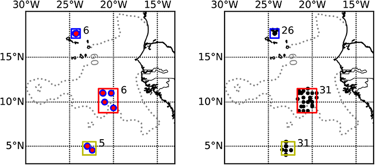
Figure 1. Map showing the sampling area in the ETNA and the three sampling regions. Boxes indicate the area boundaries from which CTD or ADCP data were included in the analysis (blue: CVOO, red: cOMZ, yellow: 5N). (Left) Multinet deployments. (Right) CTD deployments. Numbers next to the boxes indicate the number of day-night multinet pairs or CTDs obtained in the respective region. Within the cOMZ, a random subsampling was conducted to reduce the number of CTD profiles used to 31. Gray dotted contour line indicates 60 $\mu mol{O}_{2}k{g}^{-1}$ oxygen (World Ocean Atlas 2018) at 400 m depth. Lower values are found at cOMZ.

TABLE 1

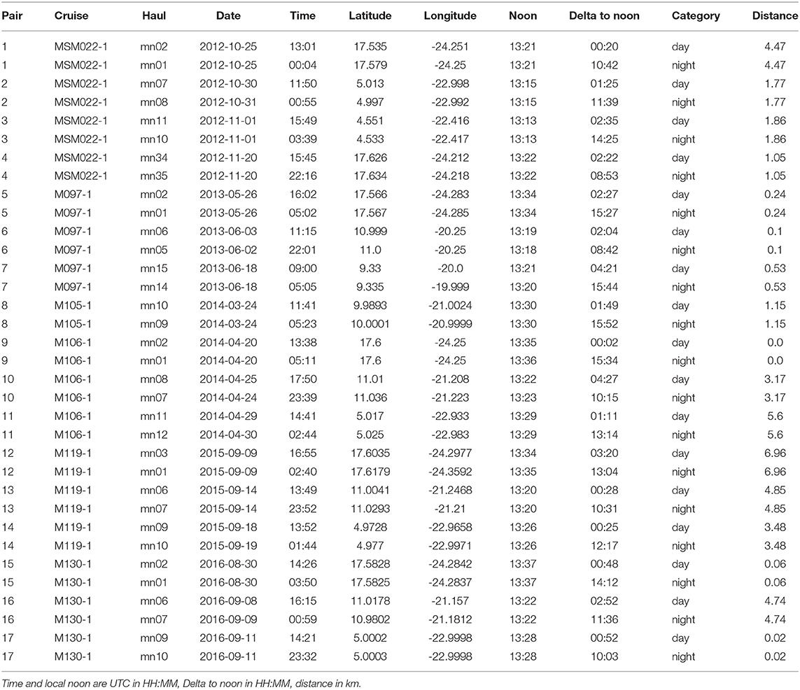
Table 1. Metadata for each pair of hauls used in this publication.

2.2. Laboratory Analysis of Multinet Catches

Samples were fixed in borax-buffered formaldehyde in seawater solution and brought to the home laboratory. Here, each sample was size-fractionated (small: 200–500 μm, medium: 500–1, 000 μm and large: > 1, 000 μm). The small fraction was not further used in this analysis. For the medium fraction, subsamples with about 1,000 zooplankton items per subsample were generated using a Motoda Splitter, whereas the entire large fraction was used for further analysis. The plankton items contained in each fraction were distributed and separated on a 20*30 cm glass tray and the glass tray scanned using an Epson perfection V750 pro flatbed scanner. Object segmentation was conducted using Zooprocess (Gorsky et al., 2010) and taxonomic units were assigned automatically using Plankton Identifier or the prediction options in EcoTaxa (Picheral et al., 2017). Assignments were thereafter corrected manually on the EcoTaxa platform. Analysis of the biovolume-size spectrum (Figure S1) showed that organisms with an equivalent spherical volume smaller than 0.032 mm⁻³ (equivalent to a equivalent spherical diameter of 0.39 mm) and larger than 4,188 mm⁻³ (equivalent to an equivalent spherical diameter of 20.0 mm) were not quantitatively sampled. We therefore excluded these from further analysis. See Figure S1 for further details. Taxon-specific area-to-drymass conversion factors for subtropical zooplankton (Lehette and Hernández-León, 2009) and drymass to carbon (C) and nitrogen (N) conversion factors (Kiørboe, 2013) were used to calculate the biomass, C and N content of each zooplankton organism scanned. Taxonomic units and biomass conversion factors used are listed in Table 2. Abundance and biomass estimates are lower bounds, as some organisms touched each other (multiple) or were entangled in an indiscernable mass with detritus. We consider the following categories to be well conserved and constrain our analyses on these: crustacea, chaetognatha, calycophoran siphonophores, annelida, and mollusca. Fish are also well-conserved, but not included in the literature on zooplankton individual biomass estimates or metabolic rates (Lehette and Hernández-León, 2009; Kiørboe, 2013; Ikeda, 2014) we use. The following categories can not be quantitatively evaluated, as many of their members are either damaged by the net or the fixation: all rhizaria, thaliacea, ctenophores, cnidaria other than calycophoran siphonophores. Our estimates of total biomass as well as zooplankton-mediated fluxes should therefore be considered lower bound estimates.

TABLE 2

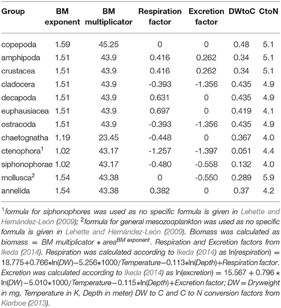
Table 2. Conversion factors and functions used in this publication.

2.3. Calculation of Mesozooplankton Biomass, Metabolic Activity, and Mortality

Taxon-specific equations for biomass and temperature dependence of respiration and ammonium excretion (Ikeda, 2014) were applied to calculate the depth-specific respiration and ammonium excretion rate of each scanned specimen (see Table 2 for equations and taxon specific factors used). The average temperature for the sampled depth layer was obtained from the concomitant CTD deployments. The environmental pO₂ was generally much higher than the estimated p_crit for migrating euphausiids and copepods (Kiko et al., 2016, see also Figure 2). Therefore, unlike to our companion paper (Kiko and Hauss, 2019), we did not apply a correction of oxygen-dependent depression of metabolic activity. Daily mortality of copepods was calculated according to Hirst and Kiørboe (2002) as ln(mortality) = 0.047*Temperature−0.154*ln(DW)−2.532, thereby treating all copepods as broadcast spawners (DW = Dryweight in μg, Temperature in Celsius). Mortality of all other groups was calculated according to Hirst and Kiørboe (2002) as log10(mortality) = (−0.325*log10(DW)−0.154)/2^{(15−temperature)/10}, thereby applying a Q10 of 2 (DW = Dryweight in g, Temperature in Celsius). Individual daily mortality was multiplied with the individual biomass and summed up to yield mortality per day in mg Carbon. Day-night differences of total respiration, ammonium excretion and mortality were calculated for each depth level in order to include effects of temperature and size-distribution. For depth below 100 m, these day-night differences coincide with the migratory fluxes. Migratory losses from the 0 to 200 m depth layer were calculated as the sum of the integrated day-night difference of fluxes at 200 to 1,000 m depth to avoid artifacts due to sampling net avoidance in the surface layer at daytime (Ianson et al., 2004) and reduction of metabolic activity at depth due to lower temperatures. A residence time at depth of 12 h was assumed. To test for statistical significance of day-night differences, a one-sided students t-Test against zero was conducted (p < 0.05).

FIGURE 2

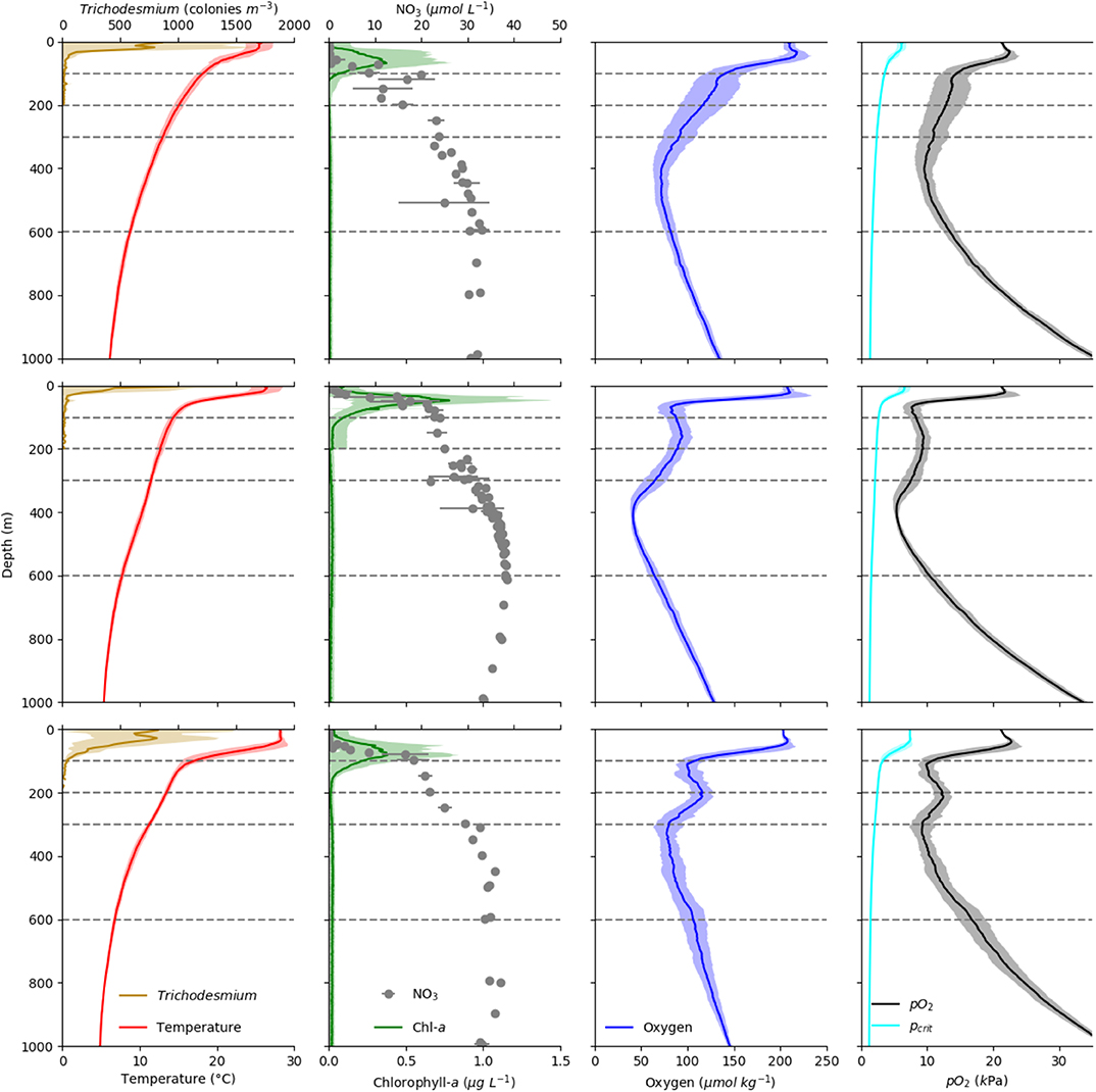
Figure 2. Vertical profiles of Temperature (°C, red line), Trichodesmium sp. abundance (individuals m⁻³, yellow line), Chlorophyll-a (mg m⁻³, green line), Nitrate concentration ($\mu mol{O}_{2}k{g}^{-1}$, gray dots), oxygen concentration ($\mu mol{O}_{2}k{g}^{-1}$, blue line), and pO₂ (kPa, black line) as well as estimated p_crit (kPa, cyan line) of the migrating euphausiid species Euphausia gibboides in the three regions CVOO (top), cOMZ (middle), and 5N (bottom). Dashed lines indicate the depth strata of our multinet deployments.

2.4. Calculation of POC Content and POC Flux From UVP5 Data

High-resolution full depth particle size spectra (0.14–44 mm equivalent spherical diameter, ESD) were obtained with an Underwater Vision Profiler 5 (UVP5 Picheral et al., 2010), mounted on the CTD-Rosette used during the respective cruise. Calculating POC flux from UVP5 data relies on assumptions about the relationship between particle size and POC content and particle size and sinking speed (Kriest, 2002; Giering et al., 2020). These vary widely with particle type and regional estimates of particle flux from sediment traps should be used to validate the UVP5 derived POC flux estimates (Guidi et al., 2008). We therefore calculated POC flux using parameterizations proposed by Kriest (2002), Guidi et al. (2008), and Iversen et al. (2010) (see Figure S2) and compared these to published POC flux measurements from the region (Engel et al., 2017; Hernández-León et al., 2019) obtained with surface-tethered sediment traps. The parameterization by Iversen et al. (2010) leads to a strong overestimation of POC flux, whereas the parameterization of Guidi et al. (2008) leads to an underestimation. Only the parameterization by Kriest (2002) fits the data reasonably well and matches the data from Hernández-León et al. (2019) almost perfectly. Data obtained by Engel et al. (2017) coincide well at depth, but are generally higher in the surface area. In both cases surface tethered sediment traps were used, but Hernández-León et al. (2019) deployed only one trap, whereas Engel et al. (2017) deployed a chain of traps. It is likely that surface tethered trap chains are not moving freely with the surface current, as their deeper traps act as a drogue, and therefore the upper traps are experiencing drag through the water column. Thus, (a) the individual traps might hang shallower than determined with the given rope length, and (b) traps at different depths might show differing trapping efficiencies, as they might experience different current speeds and be tilted differently. Buesseler et al. (2000) observed that a chain of traps indicated a strong flux attenuation with depth, which was not observed in parallel deployments of neutrally buoyant traps. They suggest that surface tethered trap chains might overestimate sedimenting flux by up to 30%. Given these uncertainties, we decided to use the parameterization by Kriest (2002) to calculate POC content and flux from UVP5 data. This parameterization assumes that particle mass and sinking speed can be calculated using empirically derived relationships for marine aggregates (see Kriest, 2002, reference 2a of Table 1 and reference 9 of Table 2 for mass and sinking speed of a particle, respectively). Assuming a C:N ratio of 106:16, this yields an expression for the sinking flux (in mg C m d⁻¹) of a single particle characterized by its diameter ESD (in cm) of 2.8649*ESD^2.24. Multiplying with the particle number in a particle size class (in particles m⁻³), and integrating over all size classes between 0.13 and 1 mm, we obtain the total POC flux (mg C m⁻² d⁻¹) for this size range. This parameterization was derived from in situ measurements of particulate matter sinking speeds and carbon content and has been shown to best reproduce profiles of marine snow and particulate organic matter at the same time (Kriest, 2002). To calculate the POC flux, we here use the total abundance of all objects of 0.13–1 mm size as it is not possible to discern different objects in this size range. Images of all objects larger than 1 mm were sorted into feces, aggregates and other classes (e.g., copepods, rhizarians etc.) using EcoTaxa (https://ecotaxa.obs-vlfr.fr). POC content and flux were calculated for each single feces or aggregate item using above described formula and added to the POC-flux calculated for the 0.13–1 mm fraction to yield the total flux. The largest detritus item observed had an equivalent spherical diameter of 44 mm.

2.5. ADCP Data Analysis

During the cruises M105, M106, M119, and M130 a 38 kHz RDI Ocean Surveyor (OS38) was mounted in the ship's sea chest and worked continuously. Depending on the region and sea state, the range covered by the instruments is around 1,000 m. The minimum size of particles that influences the sound scattering of the OS38 are 10–20 mm therefore, large copepods, euphausiids and small pelagic fishes contribute most to the backscatter amplitude recorded by the OS38. To investigate the vertical migration of the zooplankton the echo amplitude of the OS38 was transformed into volumetric backscatter Sv (dB) (Mullison, 2017) to correct the depth dependency of the data. Furthermore, Sv between 10:00 to 14:00 and 22:00 to 2:00 o'clock local time were selected for every 24 h and averaged in daytime and nighttime profiles. To obtain the difference in volumetric backscatter the daytime values were subtracted from the nighttime values. In addition a two-sample t-Test was applied (p-value <0.05) to identify in which depths the day and night-time values were significantly different.

2.6. Model Setup

To investigate the potential necessity to include zooplankton gut flux and respiration in global models we here investigate a global biogeochemical model (Kriest and Oschlies, 2015, setup RemHigh) that was designed to represent the oxidant cycles in OMZs, but excludes vertical migration of zooplankton. The biogeochemical model was coupled to a global offline circulation model based on the Transport Matrix Method (Khatiwala, 2007), using 12 monthly mean transport matrices derived from the Estimating the Circulation and Climate of the Ocean (ECCO) project, which provides circulation fields that yield a best fit to hydrographic and remote sensing observations over a 10-year period (). The global model has a horizontal resolution of 1° × 1° with 23 vertical levels in the vertical. Three model configurations with different power-law exponents (analogous to Martin et al., 1987) describing the particle flux to the ocean interior b (0.6435, 0.858, and 1.0725) were simulated over 9000 years, i.e., until near steady state. In addition we test a biogeochemical model configuration in the same circulation, in which we optimized six biogeochemical parameters of the coupled global model against observed nutrients and oxygen. Optimization was carried out as described by Kriest et al. (2017). Optimized b was estimated at 1.46. The other optimal parameters and further details of model performance can be found in Kriest et al. (2020).

3. Results

3.1. Environmental Conditions at the Three Sampling Regions

Temperature profiles in the surface layers at 5N, cOMZ, and CVOO are markedly different (Figure 2). The mixed layer was deepest and sea surface temperature highest at 5N. Beneath, a uniform temperature of approximately 27–28°C was found in the upper 40 m at 5N, which then declined to a mean (± SD) of 17.0 (± 1.6)°C at 100 m depth, whereas mixed layer temperatures at cOMZ and CVOO were slightly lower (approximately 25–26°C at cOMZ and 23–25°C at CVOO) and declined gradually to 14.4 (± 0.5) and 18.2 (± 0.7)°C at 100 m depth at cOMZ and CVOO, respectively. The colder temperatures at cOMZ at 100 m are due to a shallowing of the isopycnals associated with the presence of the Guinea Dome. Temperature profiles between 100 and 1,000 m depth were rather similar, with temperatures in the 300–600 m depth layer ranging between 8.8 and 13.0 (CVOO; median: 10.6), 7.7 and 11.5 (cOMZ; median 9.6), and 6.8 and 11.2 (5N; median 8.4) °C, respectively. The chlorophyll a maximum was shallowest at cOMZ and deepest at 5N. Integrated chlorophyll a concentrations were lowest at 5N with a mean of 26.7 mg m⁻² (Standard Error = 3.2, n = 30), and similar at CVOO (27.6 mg m⁻², SE = 4.6, n = 17) and highest at cOMZ (35.4 mg m⁻², SE = 3.7, n = 31). This observation was in line with the nitracline depth. Mean nitrate concentrations exceeded 15 μmol L⁻¹ at 45, 75, and 100 m depth at cOMZ, 5N, and CVOO, respectively. Trichodesmium sp. abundance was by far highest at 5N, with a mean integrated abundance of 43.7 *10³ colonies m⁻², while 24.4 and 15.5*10³ colonies m⁻² were observed at CVOO and cOMZ, respectively. Primary productivity estimates from satellite data (https://www.science.oregonstate.edu/ocean.productivity/) obtained within the same week (8-day time window) as the CTD profiles were found to be 490.1 ±82.6 sd (5N), 679.4 ±322.2 sd (cOMZ), and 510.1±108.4 sd (CVOO) mg C m⁻² d⁻¹. In addition also the oxygen profiles in the three regions differ, with a pronounced subsurface OMZ and a fully developed midwater OMZ at 5N and cOMZ, with the latter reaching lower oxygen concentrations. Oxygen partial pressure is first of all a function of oxygen concentration, but also impacted by temperature and salinity, with lower partial pressures at higher temperatures and salinities. The decline of temperature with depth therefore leads to a tilted pO₂ profile in comparison to the oxygen concentration profile. Both 5N and cOMZ feature two pO₂ minima, the first at 100 m depth and the second at 300 and 400 m depth at 5N and cOMZ, respectively. At 5N, pO₂ dropped to about 9.2 kPa in the two minima, whereas they lie at about 5.4 kPa at cOMZ. At CVOO, only one pO₂ minimum with a value of about 9.6 kPa was observed at about 400 m depth. Mean pO₂ values were below or very close to 10 kPa between 50 and 600 m depth at cOMZ throughout, between 100 and 150 and about 270–400 m depth at 5N, and between about 325–470 m depth at CVOO. At none of the stations, the pO₂ fell below the extrapolated p_crit of E. gibboides (Figure 2).

3.2. Mesozooplankton Biomass Distribution

Integrated biomass of well-preserved zooplankton (size range 0.39–20.00 mm) calculated from day and night hauls was highest at cOMZ (1589.7 mg C m⁻²) and comparatively low at both CVOO and 5N (987.8 mg C m⁻² and 685.7 mg C m⁻², respectively, Table 3). Daytime biomass was high at the surface, declined in the 100–200 and 200–300 m depth layers and then increased again slightly in the 300–600 m depth layer at 5N and CVOO, whereas it increased markedly in this depth layer at cOMZ (Figure 3, Table S2). Low biomass values were again found in the 600–1,000 m depth layer at daytime, but they were also low at nighttime. Biomass in the 300–600 m depth layer was lower at nighttime at all three stations, but a significant deviation from zero in the daytime minus nighttime biomass was only found at cOMZ (One-sided Students t-Test, p < 0.05). Here, median nighttime biomass was 2.0-fold higher than daytime biomass. Increases in nighttime biomass were observed in the 100–200 and 0–100 m depth layer. Highest median biomass (9.5 mg C m⁻³; quartiles: 8.7 mg C m⁻³, 10.1 mg C m⁻³) was observed in the 0–100 m depth layer at cOMZ. Crustaceans contributed most to biomass at all depths and increased from a median contribution of 54 (CVOO), 80 (cOMZ) and 83 % (5N) in the 0–100 m depth layer to a median contribution of 95 (cOMZ), 95 (CVOO), and 83 % (5N) in the 300–600 m depth layer (Table S3). Within crustaceans, copepods and euphausiids were the major contributors to biomass (data not shown). The day-nighttime biomass difference at 300–600 m depth was almost exclusively related to the difference in crustacean biomass. Mortality expressed as biomass in mg C lost per day and cubic meter follows very similar patterns as the biomass distribution itself. Detailed values can be found in Table S4. Figure S3 shows the respective plots.

TABLE 3

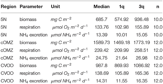
Table 3. Biomass, respiration, and excretion estimates integrated for the upper 1,000 m at the three sampling locations.

FIGURE 3

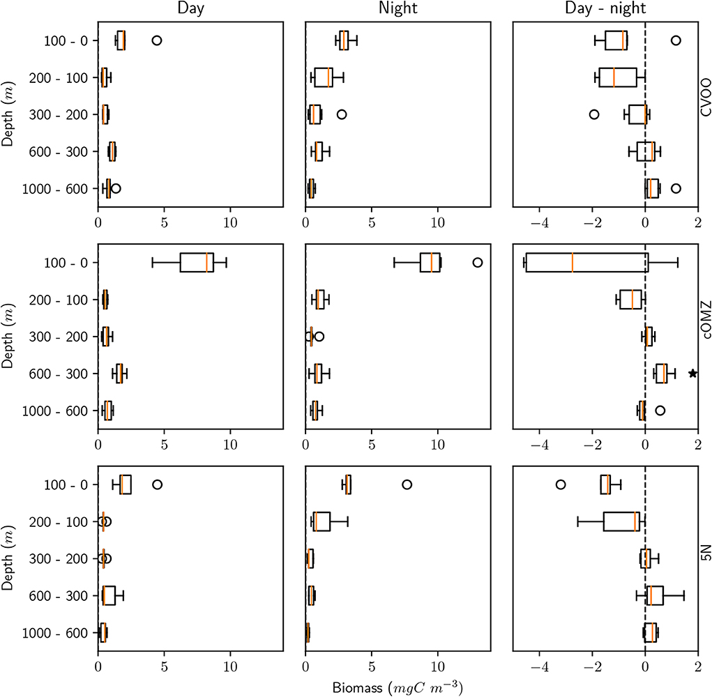
Figure 3. Mesozooplankton biomass for day, night, and the day-night difference in each layer and for the three different sampling regions. An asterisk (*) denotes a significant difference (one-sided Students t-test, p < 0.05) of the day-night difference from zero.

3.3. Mesozooplankton Ammonium Excretion and Respiration

Ammonium excretion and respiration rates followed similar patterns as the biomass distribution patterns. Median ammonium excretion rates integrated for the 1,000–0 m depth layer sampled were comparatively low at 5N and CVOO (13.4 $\mu molN{H}_4{m}^{-2}{d}^{-1}$ and 14.3 $\mu molN{H}_4{m}^{-2}{d}^{-1}$, respectively), whereas median rates were almost twice as high at cOMZ (24.8 $\mu molN{H}_4{m}^{-2}{d}^{-1}$, Table 3). Likewise, integrated respiration rates of 133.8 $\mu mol{O}_2{m}^{-2}{d}^{-1}$ and 138.7 $\mu mol{O}_2{m}^{-2}{d}^{-1}$ were found at 5N and CVOO, respectively, and almost twice as high values at cOMZ (239.4 $\mu mol{O}_2{m}^{-2}{d}^{-1}$, Table 3). Daytime ammonium excretion rates in the upper 100 m were 1.53 $\mu molN{H}_4{m}^{-3}{d}^{-1}$ at 5N and 1.49 $\mu molN{H}_4{m}^{-3}{d}^{-1}$ at CVOO (Figure 4, Table S5), respiration rates were 15.6 $\mu mol{O}_2{m}^{-3}{d}^{-1}$ (5N) and 12.6 $\mu mol{O}_2{m}^{-3}{d}^{-1}$ (CVOO; Figure 5, Table S6). Approximately three times higher rates were observed at cOMZ (ammonium excretion rate 4.44 $\mu molN{H}_4{m}^{-3}{d}^{-1}$, respiration rate 39.9 $\mu mol{O}_2{m}^{-3}{d}^{-1}$). Nighttime surface excretion rates increased to 2.74 $\mu molN{H}_4{m}^{-3}{d}^{-1}$ (5N), 2.25 $\mu molN{H}_4{m}^{-3}{d}^{-1}$ (CVOO), and 4.79 $\mu molN{H}_4{m}^{-3}{d}^{-1}$ (cOMZ), whereas respiration rates increased to 29.4 $\mu mol{O}_2{m}^{-3}{d}^{-1}$ (5N), 21.8 $\mu mol{O}_2{m}^{-3}{d}^{-1}$ (CVOO), and 48.3 $\mu mol{O}_2{m}^{-3}{d}^{-1}$ (cOMZ). Excretion and respiration rates at 300 to 600 m depth were substantially reduced and values are very similar, with median values ranging between 0.1 $\mu molN{H}_4{m}^{-3}{d}^{-1}$ and 0.2 $\mu molN{H}_4{m}^{-3}{d}^{-1}$ for ammonium excretion and between 0.9 $\mu mol{O}_2{m}^{-3}{d}^{-1}$ and 2.8 $\mu mol{O}_2{m}^{-3}{d}^{-1}$ for respiration in all regions. The day-night excretion and respiration rate difference at depth was only significantly different from zero in the cOMZ region, where the day excretion and respiration rates were higher than the night rates (with a difference of 0.05 $\mu molN{H}_4{m}^{-3}{d}^{-1}$ and 0.6 $\mu mol{O}_2{m}^{-3}{d}^{-1}$, respectively).

FIGURE 4

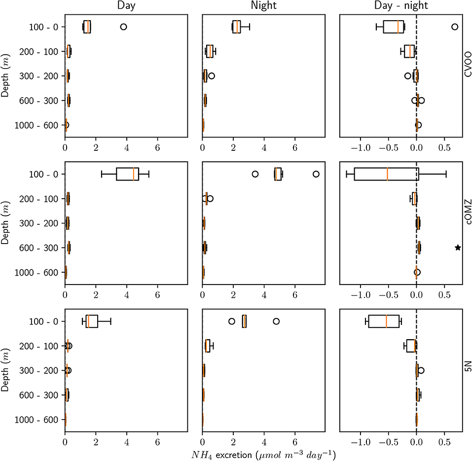
Figure 4. Mesozooplankton ammonium excretion for day, night and the day-night difference in each layer and for the three different sampling regions. An asterisk (*) denotes a significant difference (one-sided Students t-test, p < 0.05) of the day-night difference from zero.

FIGURE 5

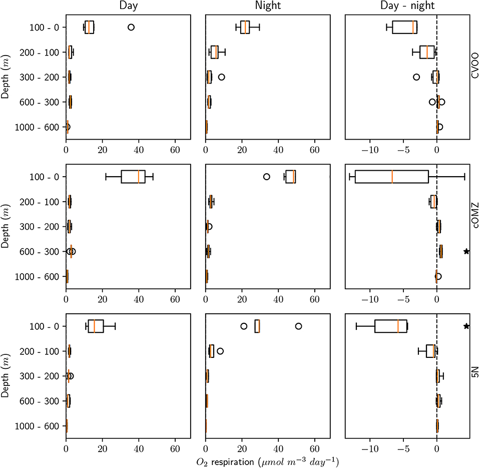
Figure 5. Mesozooplankton respiration for day, night, and the day-night difference in each layer and for the three different sampling regions. An asterisk (*) denotes a significant difference (one-sided Students t-test, p < 0.05) of the day-night difference from zero.

3.4. POC Content and Flux From in situ Particle Imaging

POC content and flux calculated from UVP5 data (Figure 6, Table 4) varies markedly between the three investigation areas. Average POC content in the surface area (0–100 m depth) was highest at cOMZ (average 2.9 ± 1.2 mg C m⁻³, n = 30), followed by 5N (average 2.6 ± 0.9 mg C m⁻³, n = 31) and then CVOO (average 2.2 ± 0.7 mg C m⁻³, n = 26). In all regions the POC content is substantially lower in the 100–200 and 200–300 m depth layer. Whereas the average POC content declines further in the 300–600 m depth layer at CVOO to average values of 0.8 ± 0.1 mg C m⁻³, n = 22, it increases again slightly at 5N (average 0.5 ± 0.1 mg C m⁻³, n = 24) and markedly at cOMZ (0.9 ± 0.1 mg C m⁻³, n = 27), thus resembling an intermediate particle maximum (IPM) in the OMZ core. POC content declines again rather gradually below about 500 m depth in all three regions. Mean POC content in the 600–1,000 m depth layer is highest at cOMZ (average 0.7 ± 0.1 mg C m⁻³, n = 27), followed by CVOO (average 0.6 ± 0.1 mg C m⁻³, n = 22), and 5N (average 0.5 ± 0.1 mg C m⁻³, n = 24). POC flux follows similar patterns, but the flux increase at midwater depth is less pronounced (cOMZ) or barely visible (5N and CVOO). Detailed POC flux values for the described depth layers can be found in Table 4. POC flux at 200 m depth (average of the values observed between 190 and 210 m depth) amounts to 9.3 mg C m⁻² d⁻¹, 18.1 mg C m⁻² d⁻¹, and 16.4 mg C m⁻² d⁻¹ at 5N, cOMZ and CVOO, respectively. POC flux at 300 m depth (average of the values observed between 290 and 310 m depth) is highest at cOMZ (16.2 mg C m⁻² d⁻¹), where it declines to 14.1 mg C m⁻² d⁻¹ at 600 m (average of the values observed between 590 and 610 m depth). POC flux at 300 m depth at CVOO is slightly lower (14.8 mg C m⁻² d⁻¹) and declines to 11.1 mg C m⁻² d⁻¹ at 600 m depth. Lowest POC flux at 300 m depth is observed at 5N with 9.1 mg C m⁻² d⁻¹ and slightly lower values at 600 m depth (7.4 mg C m⁻² d⁻¹).

FIGURE 6

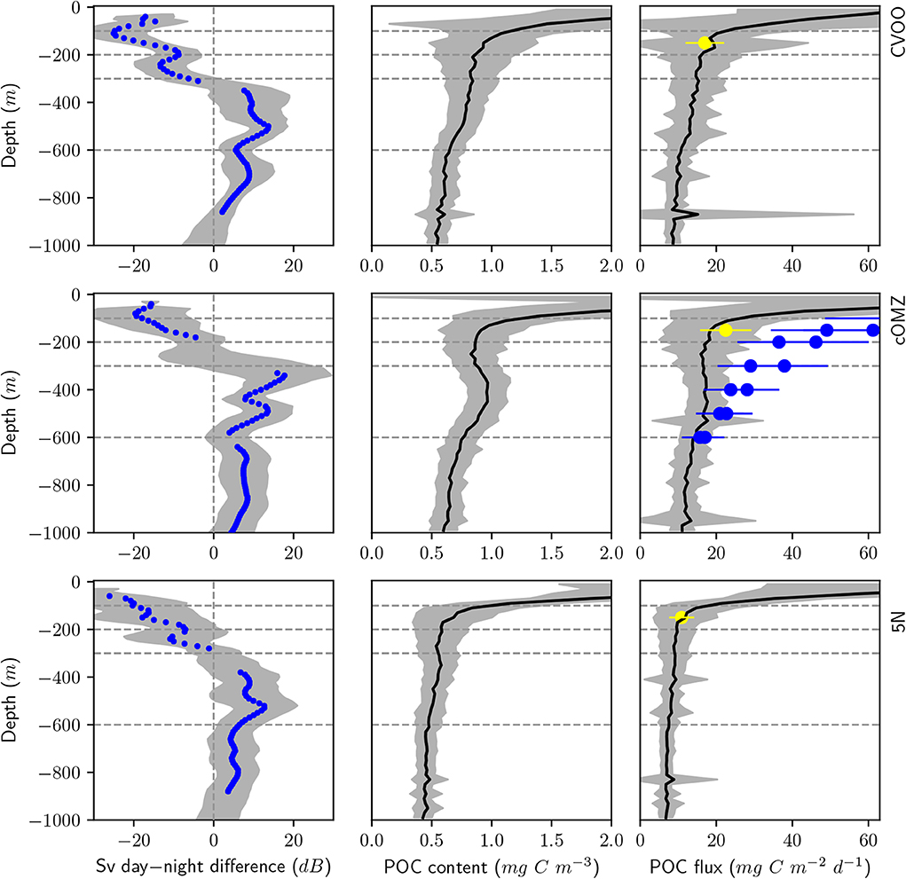
Figure 6. Day-night backscatter difference from the vessel mounted 38 kHz ADCP (left), average POC content (middle), and POC flux (right) from UVP5 data obtained during CTD deployments in the respective regions. Top panels: CVOO, Middle panels: cOMZ, Bottom panels: 5N. Gray shading indicates the standard deviation of the respective parameter. Blue dots in the left panels indicate the mean ADCP backscatter if the day and night values are significantly different from each other. Blue dots in the right panels indicate sediment trap data from Engel et al. (2017), yellow dots indicate sediment trap data from Hernández-León et al. (2019). An approximate 30% uncertainty of sediment trap estimates is indicated with error bars. Dashed lines indicate the depth levels of our multinet deployments.

TABLE 4

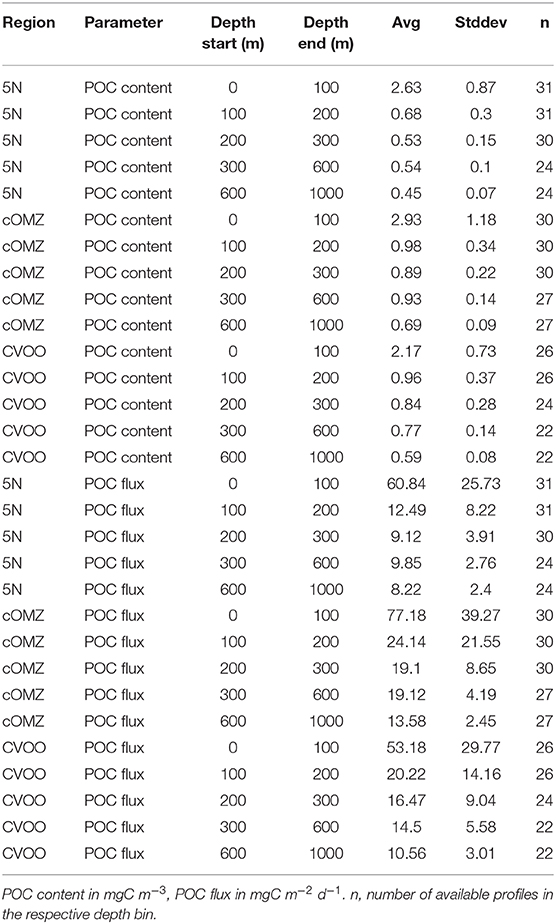
Table 4. Average values and standard deviation of POC content and POC flux calculated from UVP5 data for the five depth layers of interest.

3.5. Nitrogen Fluxes Out of the Top 200 m

The median active export of dissolved ammonium via DVM from the 0 to 200 m depth layer can be estimated at 10.9 μmol N m⁻² d⁻¹ (5N), 15.1 μmol N m⁻² d⁻¹ (cOMZ), and 12.8 μmol N m⁻² d⁻¹ (CVOO; Figure 7). These values are calculated as the sum of integrated differences for the 200–1,000 m depth layer. The DON export calculated assuming a DON excretion to ammonium excretion ratio of 0.32 Steinberg et al. (2002) is estimated at 3.5 μmol N m⁻² d⁻¹ (5N), 4.8 μmol N m⁻² d⁻¹ (cOMZ), and 4.1 μmol N m⁻² d⁻¹ (CVOO) μmol DON m⁻² day⁻¹. Estimating the active N gut flux as a result of defecation at 1% of the migrating biomass [calculated from Schnetzer and Steinberg (2002)] and the N loss at depth due to mortality with the allometric equations provided by Hirst and Kiørboe (2002) results in a flux of 56.6 μmol N m⁻² d⁻¹ (5N), 67.9 μmol N m⁻² d⁻¹ (cOMZ), and 69.1 μmol N m⁻² d⁻¹ (CVOO) μmol N m⁻² day⁻¹ out of the 0–200 m depth layer (for detailed mortality estimates see Table S4), values are converted from C to N using a Redfield ratio of 106 C : 16 N). Combined with the fluxes due to excretion these values add up to a loss of 70.9 μmol N m⁻² d⁻¹ (5N), 87.9 μmol N m⁻² d⁻¹ (cOMZ), and 86.0 μmol N m⁻² d⁻¹ (CVOO) μmol N m⁻² day⁻¹ due to DVM-related processes. Converting passive POC sinking fluxes at 200 m depth to PON fluxes using a Redfield ratio of 106 C: 16 N results in 100.4 μmol N m⁻² day⁻¹, 195.1 μmol N m⁻² day⁻¹, and 176.3 μmol N m⁻² day⁻¹ at 5N, cOMZ, and CVOO, respectively. DVM-mediated losses make up 32 (CVOO), 31 (cOMZ), and 41 (5N) % of total N-loss at 200 m depth.

FIGURE 7

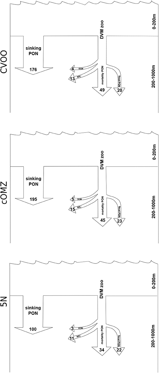
Figure 7. Nitrogen fluxes out of the upper 200 m for the three regions. All values in μmol N m⁻³ day⁻¹. Estimate of the sinking PON flux is the average from our UVP5 data calculated for 190–210 m depth. Zooplankton related DVM fluxes (DVM zoo) are the median fluxes calculated from the sum of integrated day-night differences observed in the 200–300, 300–600, and 600–1,000 m depth layers.

3.6. Carbon and Oxygen Fluxes at Midwater Depth

Active carbon supply to the 300–600 m depth layer via DVM gut flux, mortality and DOC excretion [calculated as 31% of respiration, Steinberg et al. (2000)] amounts to 243.6 $\mu mol{O}_2{m}^{-2}da{y}^{-1}$ (CVOO), 444.3 $\mu mol{O}_2{m}^{-2}da{y}^{-1}$ (cOMZ), 169.6 $\mu mol{O}_2{m}^{-2}da{y}^{-1}$ (5N) (Figure 8; all values shown are converted to μmol O₂ using a respiratory quotient of 0.86 to allow for comparison with the oxygen demand). Passive flux amounts to 1057.1 $\mu mol{O}_2{m}^{-2}{d}^{-1}$ (CVOO), 1158.8 $\mu mol{O}_2{m}^{-2}{d}^{-1}$ (cOMZ), and 652.4 $\mu mol{O}_2{m}^{-2}{d}^{-1}$ (5N) at 300 m depth, whereas it amounts to 795.3 $\mu mol{O}_2{m}^{-2}{d}^{-1}$ (CVOO), 1012.1 $\mu mol{O}_2{m}^{-2}{d}^{-1}$ (cOMZ), and 527.7 $\mu mol{O}_2{m}^{-2}{d}^{-1}$ (5N) at 600 m depth. 32 (CVOO), 31 (cOMZ), and 41% (5N) of the total flux into the 300–600 m depth layer are DVM-mediated. For the 300–600 m depth stratum, we estimate median integrated respiration rates of 510.0 $\mu mol{O}_2{m}^{-2}da{y}^{-1}$, 480.0 $\mu mol{O}_2{m}^{-2}da{y}^{-1}$, and 270.0 $\mu mol{O}_2{m}^{-2}da{y}^{-1}$ of resident zooplankton (calculated from nighttime hauls only) at CVOO, cOMZ, and 5N, respectively. Integrated migratory oxygen demand can be estimated at 90.0 $\mu mol{O}_2{m}^{-2}da{y}^{-1}$ (CVOO), 180.0 $\mu mol{O}_2{m}^{-2}da{y}^{-1}$ (cOMZ), and 60.0 $\mu mol{O}_2{m}^{-2}da{y}^{-1}$ (5N).

FIGURE 8

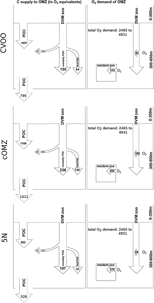
Figure 8. Carbon supply and oxygen demand budget of the 300–600 m depth layer for the three regions. Carbon supply is converted to oxygen equivalents using a respiratory quotient of 0.86. All values in $\mu mol{O}_2{m}^{-2}da{y}^{-1}$. POC flux is the average from our UVP5 data calculated for 290–310 m and 590–610 m depth. All zooplankton related rates are median values. Total oxygen demand from Karstensen et al. (2008) (3–6 $\mu mol{O}_{2}k{g}^{-1}yea{r}^{-1}$ converted $\mu mol{O}_2{m}^{-2}da{y}^{-1}$).

3.7. Comparison to Model Results

We here compare observed oxygen concentration and organic matter flux via sinking particles to our model results with the coupled global biogeochemical model MOPS (Kriest and Oschlies, 2015) in Figure 9. In sensitivity experiments carried out by Kriest and Oschlies (2015) the power-law exponent describing the particle flux to the ocean interior b was increased from b = 0.6435 over b = 0.858 to b = 1.0725, i.e., from deep to shallower remineralization of particulate organic matter. In agreement with observations, all model experiments exhibit a steep subsurface decline of oxygen, down to values of about 30 mmol m⁻³ in the optimized model. However, no model setup reflects the double OMZ observed at cOMZ and 5N. Even objective parameter optimization against global data sets of nutrients and oxygen (as carried out by Kriest et al., 2020) does not yield any significant improvement at the three locations analyzed here. At CVOO and cOMZ the optimized model and the experiment with relatively shallow remineralization (as represented by b = 1.0725) show a good match to the observed oxygen below 400 m. On the other hand, at 5N the best fit to observed oxygen is obtained with b = 0.858 or less. Thus, CVOO and cOMZ, the two regions with stronger zooplankton migration and respiration (Figure 8), require model setups with rather shallow remineralization in order to match oxygen between ≈ 400-600 m, while the region at 5N is simulated best with the “classical” exponent of b = 0.858 (Martin et al., 1987).

FIGURE 9

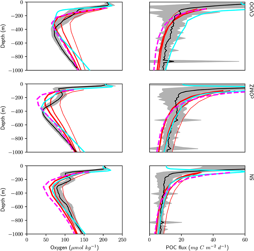
Figure 9. Simulated (red, magenta, and cyan) and observed (black and gray) oxygen (left) and POC flux (right) below 100 m depth averaged over the three different regions CVOO (top), cOMZ (middle), and 5N (bottom). Model results are annual means of year 9000 of simulation RemHigh (Kriest and Oschlies, 2015) with three different exponents b for the particle flux curve. Thick red lines: b = 1.0725; medium red lines: b = 0.858; thin red lines: b = 0.6345. Magenta dashed lines show results of the same model optimized against observed nutrients and oxygen (Kriest et al., 2020). Cyan lines show results from Aumont et al. (2018).

Deep particle flux at CVOO is represented best by a particle flux with a b value between 0.6345 and 1.0725, even though the lower values would result in an overestimate of deep oxygen by about 20 to 40 $mmol{O}_2{m}^{-3}$ (see above). At cOMZ particle flux between 400 and 600 m (about the target depth of DVM) derived from UVP5 data is simulated best by b = 0.858; again, this value leads to an overestimate of oxygen between 400 and 600 m of about 20 mmol m⁻³. Only the model with a very steep particle flux profile (b = 0.6435) matches the trap fluxes observed by Engel et al. In this case, the model overestimates deep oxygen by ≈50 mmol m⁻³ at 400 m. Finally, at 5N observed particle flux is matched best by b defined by a range between 0.858 and 1.0725. The lowest value of b (comparable to faster settling particles) results in an overestimate of particle flux. Yet, as shown above this experiment could still produce a reasonable oxygen profile.

4. Discussion

Our work aims to provide a quantitative assessment of zooplankton biomass, diel vertical migration, and related biogeochemical fluxes in the ETNA. We here combine data from several cruises since 2012 to the region. In the following, we will first consider the constraints of optical plankton and particle assessments and the application of allometric relationships to such ocean optics data and will then discuss the derived estimates. First comparisons to model data show that independently developed models and data coincide reasonably well, but differ in important details. Our observations could be used to further constrain the models and improve parameterizations.

4.1. Estimating Biomass, Physiological Rates, and Fluxes From Ocean Optics Data—Problems and Uncertainties

Our biomass estimates of zooplankton and particles rely on empirical relationships between size and carbon or nitrogen content (Kriest, 2002; Lehette and Hernández-León, 2009), include only zooplankton that is not destroyed during net sampling and preservation in formalin and can be imaged well on a scanner. Likewise, we used allometric relationships that link size and particle sinking speed to obtain particle flux (Kriest, 2002), as well as relationships to calculate respiration, excretion and mortality rates based on size, temperature and taxonomic grouping (Hirst and Kiørboe, 2002; Ikeda, 2014). Whereas, the location and size of organisms and particles are well-defined, uncertainties of the derived estimates stem from uncertainties of the respective parameterizations. Applying such calculations is nevertheless necessary to convert the abundance and size estimates to biomass, fluxes and rates in SI units, which allows for comparison with other studies. The only parameter for which we could not find an allometric relationship is the gut flux. Here, we used data from Schnetzer and Steinberg (2002) to estimate gut flux at 1% of the migrating biomass. A general factor of 1% is not very satisfactory, as gut flux might vary according to composition and size distribution of the migrating community. The cited study was conducted at the Bermuda Atlantic Time Series Station, where the community composition may be different from the one we observed. We estimate the particulate matter supply via mortality of migrating organisms at depth by combining biomass and mortality estimates. Uncertainty with respect to this parameter is related to the fate of the dead body and the estimated mortality. Whereas natural mortality will directly contribute to the particle inventory, consumptive mortality will contribute to it via sloppy feeding and as defecation of the respective predator. Hence, the dead biomass that contributes to the POC flux might be lower than the total mortality flux. The mortality estimates we use are community estimates of consumptive and natural mortality of epipelagic communities (Hirst and Kiørboe, 2002). To our knowledge, no mortality estimates for mesopelagic zooplankton communities exist. It therefore needs to be stressed that mortality rates at depth might be different to those estimated here. However, Robison et al. (2020) note that many different, sometimes specialized mid-water predators pose a considerable threat to the migrating community. Furthermore, the migration activity itself, the changes in abiotic conditions (e.g., temperature, oxygen) and the lack of food might have so far unknown effects on the mortality of the migratory community. Natural and/or consumptive mortality might also vary regionally, depending e.g., on the oxygen level at the migration depth or the predator community composition (Robison et al., 2020). Further work, especially to parameterize zooplankton gut flux to and mortality at mid-water depth is needed and will help to reduce the uncertainties associated with the estimation of DVM-mediated fluxes. With the mentioned constraints in mind, we will in the following discuss the biomass distribution of well-preserved zooplankton and the impacts of DVM-mediated fluxes on biogeochemical cycles of nitrogen, carbon and oxygen in the ETNA.

4.2. Zooplankton Biomass Distribution

Integrated zooplankton biomass was found to be almost twice as high at cOMZ compared to 5N and CVOO. Likewise, migrator biomass was highest at cOMZ. Several indicators mark the cOMZ region as the most productive of the three regions investigated, however, none of them is changed by a factor of two. The cOMZ region is characterized by a higher integrated chlorophyll-a, as well as ocean color-derived net primary productivity, a shallower nutricline/pycnocline depth and a lower integrated Trichodesmium sp. abundance. Sandel et al. (2015) observed a lower diapycnal nutrient flux between 7 and 15°N at 23°W [a region largely coinciding with our cOMZ region; referenced to as “Guinea Dome” (GD) by Sandel et al. (2015)], compared to the Oligotrophic North Atlantic (“ONA”), which largely coincides with our 5N region and the greater CVOO region. However, these fluxes were determined across the nitracline depth, which was particularly shallow at GD, and high chlorophyll-a concentrations were still observed below this depth by Sandel et al. (2015). The elevation of the pycno- and nitracline in the GD/cOMZ region creates beneficial conditions for primary productivity, which likely is the main reason for the elevated integrated and migrating biomass in this region. Trichodesmium sp. was found to synthesize several defense molecules and therefore likely has a rather poor nutritional value for most zooplankton (Codd, 1995), which also could partly explain why zooplankton biomass is lower at 5N and CVOO, where Trichodesmium sp. is more abundant. DVM species might also benefit from the OMZ refuge at depth at cOMZ (see also Bianchi et al., 2014). Only for two endemic pelagic species in the study area p_crit values are available, E. gibboides and P. abdominalis (Kiko et al., 2016). Oxygen partial pressures at depth were found to be well above the p_crit of these species in all three regions, but only at cOMZ they are with 5.2 kPa at about 350 m depth low enough to possibly exclude fast-swimming predators with a high respiratory demand such as billfishes (Prince et al., 2010; Stramma et al., 2012) or cephalopods. In support of this hypothesis, we note that the absolute peak in day-night 38 kHz backscatter difference (an indicator for the migratory fraction of larger zooplankton like krill and nekton) actually coincides with the minimum pO₂. pO₂ minima and day-night difference peaks do not coincide at CVOO and 5N, where oxygen values are also considerably higher and a refuge due to particularly low oxygen partial pressures is therefore not created. Another reason for the observed differences might be that biomass is elevated in parts of the zooplankton size spectrum which we did not observe or in the gelatinous/fragile component of the zooplankton community.

We here specifically excluded observations obtained within mesoscale eddies that featured particularly large anomalies in any of the observed parameters. Comparison of our results to earlier work especially on low-oxygen anticyclonic modewater eddies (Karstensen et al., 2008; Fiedler et al., 2016; Hauss et al., 2016; Christiansen et al., 2018) can indicate zooplankton distribution changes we could possibly expect in the “non-eddy” situation if mean oxygen levels further decline in the ETNA. Christiansen et al. (2018) observed that the flux-feeding polychaete Poeobius sp. was particularly abundant in several anticyclonic modewater eddies with low oxygen levels in their core. The average oxygen concentration in the shallow oxygen minimum at 85 to 120 m depth of the eddy studied by Karstensen et al. (2008), Hauss et al. (2016), and Fiedler et al. (2016) was 6.6 μmol kg⁻¹ (0.56 kPa O₂). Acoustic observations (shipboard ADCP, 75kHz) revealed that larger zooplankton and nekton were avoiding this zone and were compressed at the surface (Hauss et al., 2016). In general, we therefore expect diel vertical migration activity in the ETNA to weaken if oxygen levels in the migration range fall below about $30\mu mol{O}_{2}k{g}^{-1}$. This weakening would reduce the related oxygen demand and carbon supply to the OMZ and would therefore stabilize oxygen levels, at least for some time at this level. Increases in the abundance of flux feeders such as Poeobius sp. might also occur, with strong repercussions on particle distribution and flux (Christiansen et al., 2018).

4.3. Nitrogen Flux Out of the Surface Layer

DVM mediated nitrogen loss from the surface layer (here defined as the upper 200 m, which contains the target layers of the nighttime ascent) contributes substantially to total nitrogen loss (Figure 7). Approximately 41 (5N), 31 (cOMZ), and 32% (CVOO) of the total N loss from the surface layer (PON and DVM-mediated losses combined) is lost via DVM-mediated fluxes. Such estimates are consistent with other observations (e.g., Steinberg et al., 2000, 2002; Putzeys, 2013) and highlight the importance of DVM-mediated fluxes for the nutrient budget of the surface layer. Diapycnal nitrogen supply at the 200 m depth level ranges between approximately 500 and 1,000 μmol N m⁻² day⁻¹ (Sandel et al., 2015). The given range, however, has a large uncertainty due to the sporadic occurrence of elevated mixing events in the upper thermocline associated, e.g., with shear instability of rarely occurring near-inertial waves (Bourlès et al., 2019). Nevertheless, the given range suggests that total nitrogen losses (passive flux and dvm-mediated fluxes combined) of 262.0 (CVOO), 283.0 (cOMZ), and 171.0 μmol N m⁻² day⁻¹ (5N) observed at 200 m depth are already compensated by the diapycnal supply. Sandel et al. (2015) estimate atmospheric input at about 1,000 μmol N m⁻² day⁻¹ at ONA and NCV, which largely coincide with 5N and CVOO, respectively. For the Guinea Dome region they estimate an atmospheric input of about 400 μmol N m⁻² day⁻¹. Given the large uncertainties in all these estimates, and given the fact that further loss processes, e.g. through the migration of larger organisms (Hernández-León et al., 2019) likely occur, it seems that our loss estimates are consistent with the supply estimates.

4.4. Oxygen and Carbon Budget of the DVM Target Depth

Comparing the possible active carbon supply routes via DVM gut flux, mortality, and DOC excretion with the POC supply via sedimenting particles for the three different areas investigated, we find that the carbon supply via DVM contributes 32 (CVOO), 41 (5N), and 31 % (cOMZ) to the combined supply. These results are consistent with other observations (Putzeys, 2013; Steinberg and Landry, 2017; Hernández-León et al., 2019) and highlight the importance of zooplankton mediated fluxes.

Much of the carbon supplied via passive sinking at 300 m depth is also lost this way at 600 m depth. If we calculate the relative carbon demand of the resident zooplankton considering only the POC that “disappears” at midwater depth, then we find that resident zooplankton consumes about 100 (CVOO), 81 (cOMZ), and 91 % (5N) of the supply. We do not consider the carbon demand of the migrating zooplankton in this calculation, as this should cover its carbon demand in the surface layer (Giering et al., 2014). It follows that, at least based on our assessment, only very little carbon should be available for other respiratory processes such as bacterial and microzooplankton respiration. Carbon supply at CVOO via the mechanisms investigated (POC flux and DVM-mediated processes) seems to be rather low in comparison to the likely demand. Further supply is expected to originate from larger migrators (Hernández-León et al., 2019). Lateral and vertical (via diapycnal mixing) supply of suspended and dissolved carbon might also contribute (Kelly et al., 2019). This supply pathway would mainly support the bacterial carbon demand.

Estimates of oxygen consumption at 300 to 600 m depth range between 3 and 6 $mmol{O}_2{m}^{-3}yea{r}^{-1}$ (Karstensen et al., 2008; Hahn et al., 2014). Our respiration rate estimates suggest that about 7.0 to 13.0% (5N), 12.0 to 24.0 % (CVOO), and 13.0 to 27.0 % (cOMZ) of the oxygen demand is caused by resident and migrating mesozooplankton. These estimates are somehow at odds with above described estimates of carbon supply and demand, but as mentioned, further carbon supply mechanisms need to be investigated. The estimates by Karstensen et al. (2008) include all oxygen loss and supply processes along the subduction pathway and might not represent those realized at 5N, cOMZ, or CVOO. Especially at cOMZ we would expect higher total respiration rates due to a larger POC supply compared to other regions along the subduction pathway.

4.5. Diel Vertical Migration Seems to Feed an Intermediate Particle Maximum

Particulate matter supply via gut flux, natural and consumptive mortality should contribute to the particle inventory at DVM depth. We previously reported that an equatorial Intermediate Particle Maximum (IPM) in the Atlantic and Pacific occurs at the depth of DVM activity and is strongest where day-night difference of the ADCP backscatter signal is largest. We therefore suggested that the IPM and resultant POC flux increase at midwater depth are DVM-related (Kiko et al., 2017). IPMs have been revealed by optical backscatter and turbidity, as well as UVP5 measurements in different oceanic environments (e.g., McCave, 2009; Roullier et al., 2014). They might not only be the result of zooplankton-mediated particle supply, but they could also (exclusively or additionally) be related to nepheloid layers shedding from the benthic boundary layer of coastal shelfs (Inthorn et al., 2006; Karakaş et al., 2006) and to enhanced microbial abundance in OMZs. In our current study, we also detected an IPM at 300–600 m depth at cOMZ (and to a lesser degree also at CVOO and 5N), coinciding with both the core of the OMZ and the daytime depth of DVM zooplankton. We here provide further data that suggest a link between the IPM and DVM-mediated particle supply. At cOMZ, both the IPM (as indicated by the estimated POC content) and the ADCP backscatter difference are largest and we see a significant difference to zero in the migratory zooplankton biomass obtained from our net catches. No clear IPM signal is observed at 5N and CVOO, where the ADCP backscatter signal is more stretched and smaller, and the migratory biomass difference not significant. The POC flux calculated from the particle size distribution also is clearly enhanced at 300–600 m depth at cOMZ, but not at 5N or CVOO. As we know the carbon flux into and out of the 300–600 m depth layer and the POC content (derived from the UVP5 data i.e., for the particle size range 0.14–26.8 mm) of this layer, we can derive the needed active supply of particulate matter to maintain the IPM and counter the particle remineralization. The active flux needed can be calculated as remineralisation rate * POC content + Flux out - Flux in [see also Extended data Figure 9 from Kiko et al. (2017)]. The active flux we observe at cOMZ would fully support the IPM if the remineralization rate would be 2.6% per day. Iversen and Ploug (2013) find individual particle remineralization rates of about 0.5–6% per day at 4°C. Temperatures at 300–600 m depth in the ETNA are approximately twice as high, which should increase the remineralization rate by about a factor of 1.5. As Iversen and Ploug (2013) use fresh surface material, whereas the nutritional value of material arriving at midwater depth might be more reduced, it seems reasonable that remineralization rates of 2.6% per day are possible. Considering also the uncertainties of our gut flux and mortality estimates and taking into account that we here did not consider macrozooplankton and nekton gut flux and mortality, we can not falsify the hypothesis that the IPM is a result of DVM-mediated active supply of particulate matter to depth.

4.6. Comparison to Model Results

Considering DVM-mediated fluxes at midwater depth might also improve the representation of OMZs in global biogeochemical models. We here compare model simulations by Kriest and Oschlies (2015) and Kriest et al. (2020) described above (both without DVM-mediated processes; hereafter referred to as “MOPS”), as well as results of the NEMO/PISCES/APECOSM model by Aumont et al. (2018) which does include DVM-mediated processes. Modifications of the particle settling velocity in model MOPS show that the model run with more slowly settling particles (equivalent to shallow remineralization and a large attenuation coefficient b) matches observed deep oxygen at CVOO and cOMZ, but underestimates deep particle flux, while those model runs that match observed particle flux overestimate deep oxygen by ≈20–50 mmol m⁻³.

It cannot be ruled out that the models' circulation, resolution, and possibly erroneous physical oxygen supply associated with mean advection, diapycnal mixing, and lateral eddy fluxes, causes some of the mismatches between simulated and observed oxygen. Furthermore, resident zooplankton and nekton might be underestimated in the models, which could also explain some of the mismatch. On the other hand, Bianchi et al. (2013) and Aumont et al. (2018) suggest that the impact of zooplankton on deep oxygen concentrations in highly productive upwelling areas is within the “required” range. Apparently, a considerable amount of mesopelagic remineralization is needed at CVOO and cOMZ in order to represent oxygen profiles. However, when this is achieved with a b corresponding to shallow remineralization, simulated particle flux is too low. Importantly, even after optimization of model parameters, among them the particle flux parameter b, the MOPS model is not able to simultaneously fit observed particle flux and oxygen profiles in the three regions.

In the NEMO/PISCES/APECOSM model, which parameterizes DVM, the OMZ is situated slightly deeper than in the other model experiments, but slightly shallower than in reality. Again, it remains to be investigated if and how much this feature is associated with the model physics and the distribution of resident zooplankton and nekton. The POC-flux profile actually shows a small change at the DVM-depth, which may be related to the DVM-mediated POC supply, and is supported by our observations. Therefore, in agreement with other modeling studies (Bianchi et al., 2013; Aumont et al., 2018; Archibald et al., 2019) our analysis suggests that parameterization of zooplankton and nekton diel vertical migration, its organic matter supply to the deep ocean and deep oxygen consumption can affect global and regional model performance. Comparison to our observations suggests that the NEMO/PISCES/APECOSM model still underestimates the effects, whereas the inclusion of DVM could help to improve the performance of MOPS in this region, and possibly elsewhere. Our comprehensive data set that includes zooplankton as well as particle concentrations and derived fluxes should help to further constrain such modeling efforts in terms of model parameterization, optimization, and evaluation.

4.6.1. Major Findings and Conclusions of Our Study

(1) Integrated biomass is highest at cOMZ and rather similar at 5N and CVOO. Only at cOMZ we do observe a significant day-night mesozooplankton biomass difference at 300 to 600 m depth. The oxygen levels in the three regions are not (yet) below the p_crit of two common migrators (E. gibboides and P. abdominalis). It is hence unlikely that their migration patterns are directly impacted by oxygen availability, but mesozooplankton predators might be excluded at cOMZ, creating a refuge.

(2) DVM activity removes between 31 to 41% of nitrogen from the upper 200 m of the water column. Total nitrogen loss (DVM-mediated and via passively sinking particles) from the upper 200 m of the water column is well-covered in all regions via diapycnal diffusion, nitrogen fixation, dry, and wet deposition (Sandel et al., 2015).

(3) Resident zooplankton utilizes 81 (cOMZ), 91 (5N), and 100% (CVOO) of carbon supplied to the 300–600 m depth layer via DVM and passively sinking particles (supply at 300 m minus loss at 600 m depth), indicating slightly different carbon balances in the three regions. Water column oxygen respiration at 300–600 m depth is estimated at 3–6 $mmol{O}_2{m}^{-3}yea{r}^{-1}$ (Karstensen et al., 2008) and our results indicate that zooplankton is responsible for 7–27% of it.

(4) The intermediate particle maximum is strongest at cOMZ and can probably be explained by gut flux and mortality of migrating zooplankton. Weaker impacts of diel vertical migration on the particle size spectrum can also be observed in the other regions.

(5) A first comparison of our POC-flux data to global biogeochemical model simulations indicates that the overall POC-flux estimates coincide but the contribution of DVM-mediated fluxes seems to be lacking or to be underestimated. More appropriate parameterizations might improve the representation of the biological carbon pump and the global oxygen distribution.

Data Availability Statement

Datasets analyzed in this study are available in the Pangaea collection: https://doi.pangaea.de/10.1594/PANGAEA.903023. Data not listed in this collection is available from the authors upon reasonable request. Data from scanned zooplankton images and the UVP5 is also available on https://ecotaxa.obs-vlfr.fr/.

Author Contributions

RK and HH designed the study. RK developed all routines for the biomass and metabolic rate estimation of scanned zooplankton as well as UVP5 data. RK, HH, SC, JF, and ER collected, scanned, and analyzed the zooplankton samples. PB and FS obtained and processed the CTD and ADCP data. IK designed and analyzed the biogeochemical model. RK drafted the manuscript. All authors contributed to the writing of the manuscript and agree to the submitted version.

Funding

This work is a contribution of the SFB 754 Climate—Biogeochemistry Interactions in the Tropical Ocean (www.sfb754.de, grant/award no. 27542298) which is supported by the German Science Foundation (DFG). This paper was furthermore supported by the projects TRIATLAS and iAtlantic, which have received funding from the European Union's Horizon 2020 research and innovation programme under grant agreement No 817578 and 818123, respectively. RK furthermore received a Make Our Planet Great Again grant of the French National Research Agency within the Programme d'Investissements d'Avenir; reference ANR-19-MPGA-0012.

Conflict of Interest

The authors declare that the research was conducted in the absence of any commercial or financial relationships that could be construed as a potential conflict of interest.

Acknowledgments

We are grateful to the crew and chief scientists of the research vessels Maria S. Merian and Meteor as well as the colleagues collecting nutrient data on the various cruises. Pieter Vandromme obtained Multinet samples and UVP5 data during FS Meteor cruise M119. Furthermore, we would like to thank all our colleagues of the SFB754 who supported us, provided interesting feedback regarding our work and generated a motivating work environment. Lars Stemman and Marc Picheral (Laboratoire d'Océanographie de Villefranche-sur-Mer) provided a UVP5 for cruises MSM22 and M97 and supported the optical analysis. Technical support by Hydroptic for UVP5 deployments is greatly appreciated. A special thank you also goes to the GEOMAR data management team (Hela Mehrtens, Carsten Schirnick and colleagues) and Christiane Schelten, the coordinator of the SFB754.

Supplementary Material

The Supplementary Material for this article can be found online at: https://www.frontiersin.org/articles/10.3389/fmars.2020.00358/full#supplementary-material

References

Archibald, K. M., Siegel, D. A., and Doney, S. C. (2019). Modeling the impact of zooplankton diel vertical migration on the carbon export flux of the biological pump. Glob. Biogeochem. Cycles 33, 181–199. doi: 10.1029/2018GB005983

CrossRef Full Text | Google Scholar

Auel, H., and Verheye, H. M. (2007). Hypoxia tolerance in the copepod calanoides carinatus and the effect of an intermediate oxygen minimum layer on copepod vertical distribution in the northern benguela current upwelling system and the angola-benguela front. J. Exp. Mar. Biol. Ecol. 352, 234–243. doi: 10.1016/j.jembe.2007.07.020

CrossRef Full Text | Google Scholar

Aumont, O., Maury, O., Lefort, S., and Bopp, L. (2018). Evaluating the potential impacts of the diurnal vertical migration by marine organisms on marine biogeochemistry. Glob. Biogeochem. Cycles 32, 1622–1643. doi: 10.1029/2018GB005886

CrossRef Full Text | Google Scholar

Baker, A. R., Weston, K., Kelly, S. D., Voss, M., Streu, P., and Cape, J. N. (2007). Dry and wet deposition of nutrients from the tropical atlantic atmosphere: links to primary productivity and nitrogen fixation. Deep Sea Res. Part I 54, 1704–1720. doi: 10.1016/j.dsr.2007.07.001

CrossRef Full Text | Google Scholar

Bianchi, D., Babbin, A. R., and Galbraith, E. D. (2014). Enhancement of anammox by the excretion of diel vertical migrators. Proc. Natl. Acad. Sci. U.S.A. 111, 15653–15658. doi: 10.1073/pnas.1410790111

PubMed Abstract | CrossRef Full Text | Google Scholar

Bianchi, D., Galbraith, E. D., Carozza, D. A., Mislan, K., and Stock, C. A. (2013). Intensification of open-ocean oxygen depletion by vertically migrating animals. Nat. Geosci. 6, 545–548. doi: 10.1038/ngeo1837

CrossRef Full Text | Google Scholar

Bopp, L., Resplandy, L., Orr, J. C., Doney, S. C., Dunne, J. P., Gehlen, M., et al. (2013). Multiple stressors of ocean ecosystems in the 21st century: projections with CMIP5 models. Biogeosciences 10, 6225–6245. doi: 10.5194/bg-10-6225-2013

CrossRef Full Text | Google Scholar

Bourlés, B., Araujo, M., McPhaden, M. J., Brandt, P., Foltz, G. R., Lumpkin, R., et al. (2019). Pirata: A sustained observing system for tropical atlantic climate research and forecasting. Earth Space Sci. 6, 577–616. doi: 10.1029/2018EA000428

CrossRef Full Text | Google Scholar

Brandt, P., Bange, H. W., Banyte, D., Dengler, M., Didwischus, S.-H., Fischer, T., et al. (2015). On the role of circulation and mixing in the ventilation of oxygen minimum zones with a focus on the eastern tropical North Atlantic. Biogeosciences 12, 489–512. doi: 10.5194/bg-12-489-2015

CrossRef Full Text | Google Scholar

Buesseler, K. O., Steinberg, D. K., Michaels, A. F., Johnson, R. J., Andrews, J. E., Valdes, J. R., et al. (2000). A comparison of the quantity and composition of material caught in a neutrally buoyant versus surface-tethered sediment trap. Deep Sea Res. Part I 47, 277–294. doi: 10.1016/S0967-0637(99)00056-4

CrossRef Full Text | Google Scholar

Chahsavar-Archard, V., and Razouls, C. (1982). Les copépodes pélagiques au sud-est des iles du cap vert, i. aspects qualitatifs (mission guidôme du no “j. charcot”, septembre-octobre 1976). Vie Milieu 32, 25–45.

Childress, J. J., and Seibel, B. A. (1998). Life at stable low oxygen levels: adaptations of animals to oceanic oxygen minimum layers. J. Exp. Biol. 201, 1223–1232.

PubMed Abstract | Google Scholar

Christiansen, S., Hoving, H.-J., Schütte, F., Hauss, H., Karstensen, J., Körtzinger, A., et al. (2018). Particulate matter flux interception in oceanic mesoscale eddies by the Polychaete poeobius sp. Limnol. Oceanogr. 63, 2093–2109. doi: 10.1002/lno.10926

CrossRef Full Text | Google Scholar

Cocco, V., Joos, F., Steinacker, M., Frölicher, T., Bopp, L., Dunne, J., et al. (2013). Oxygen and indicators of stress for marine life in multi-model global warming projections. Biogeosciences 10, 1849–1868. doi: 10.5194/bg-10-1849-2013

CrossRef Full Text | Google Scholar

Codd, G. (1995). Cyanobacterial toxins: occurrence, properties and biological significance. Water Sci. Technol. 32, 149–156. doi: 10.2166/wst.1995.0177

CrossRef Full Text | Google Scholar

Engel, A., Wagner, H., Le Moigne, F. A., and Wilson, S. T. (2017). Particle export fluxes to the oxygen minimum zone of the eastern tropical North Atlantic. Biogeosciences 14, 1825–1838. doi: 10.5194/bg-14-1825-2017

CrossRef Full Text | Google Scholar

Fiedler, B., Grundle, D. S., Schütte, F., Karstensen, J., Löscher, C. R., Hauss, H., et al. (2016). Oxygen utilization and downward carbon flux in an oxygen-depleted eddy in the eastern tropical North Atlantic. Biogeosciences 13, 5633–5647. doi: 10.5194/bg-13-5633-2016

CrossRef Full Text | Google Scholar

Fischer, T., Banyte, D., Brandt, P., Dengler, M., Krahmann, G., Tanhua, T., et al. (2013). Diapycnal oxygen supply to the tropical North Atlantic oxygen minimum zone. Biogeosciences 10, 5079–5093. doi: 10.5194/bg-10-5079-2013

CrossRef Full Text | Google Scholar

Giering, S. L., Sanders, R., Lampitt, R. S., Anderson, T. R., Tamburini, C., Boutrif, M., et al. (2014). Reconciliation of the carbon budget in the ocean's twilight zone. Nature 507, 480–483. doi: 10.1038/nature13123

PubMed Abstract | CrossRef Full Text | Google Scholar

Giering, S. L. C., Cavan, E. L., Basedow, S. L., Briggs, N., Burd, A. B., Darroch, L. J., et al. (2020). Sinking organic particles in the ocean-flux estimates from in situ optical devices. Front. Mar. Sci. 6:834. doi: 10.3389/fmars.2019.00834

CrossRef Full Text | Google Scholar

Gorsky, G., Ohman, M. D., Picheral, M., Gasparini, S., Stemmann, L., Romagnan, J.-B., et al. (2010). Digital zooplankton image analysis using the ZooScan integrated system. J. Plankton Res. 32, 285–303. doi: 10.1093/plankt/fbp124

CrossRef Full Text | Google Scholar

Grasshoff, K., Kremling, K., and Ehrhardt, M. (2009). Methods of Seawater Analysis. Weinheim: John Wiley & Sons.

Google Scholar

Guidi, L., Jackson, G. A., Stemmann, L., Miquel, J. C., Picheral, M., and Gorsky, G. (2008). Relationship between particle size distribution and flux in the mesopelagic zone. Deep Sea Res. Part I 55, 1364–1374. doi: 10.1016/j.dsr.2008.05.014

CrossRef Full Text | Google Scholar

Hahn, J., Brandt, P., Greatbatch, R. J., Krahmann, G., and Körtzinger, A. (2014). Oxygen variance and meridional oxygen supply in the tropical North East Atlantic oxygen minimum zone. Clim. Dyn. 43, 2999–3024. doi: 10.1007/s00382-014-2065-0

CrossRef Full Text | Google Scholar

Hahn, J., Brandt, P., Schmidtko, S., and Krahmann, G. (2017). Decadal oxygen change in the eastern tropical North Atlantic. Ocean Sci. 13, 551–576. doi: 10.5194/os-13-551-2017

CrossRef Full Text | Google Scholar

Hauss, H., Christiansen, S., Schütte, F., Kiko, R., Lima, M. E., Rodrigues, E., et al. (2016). Dead zone or oasis in the open ocean? Zooplankton distribution and migration in low-oxygen modewater eddies. Biogeosciences 13, 1977–1989. doi: 10.5194/bg-13-1977-2016

CrossRef Full Text | Google Scholar

Hauss, H., Franz, J. M., Hansen, T., Struck, U., and Sommer, U. (2013). Relative inputs of upwelled and atmospheric nitrogen to the eastern tropical North Atlantic food web: spatial distribution of δ15n in mesozooplankton and relation to dissolved nutrient dynamics. Deep Sea Res. Part I 75, 135–145. doi: 10.1016/j.dsr.2013.01.010

CrossRef Full Text | Google Scholar

Hernández-León, S., and Ikeda, T. (2005). A global assessment of mesozooplankton respiration in the ocean. J. Plankton Res. 27, 153–158. doi: 10.1093/plankt/fbh166

CrossRef Full Text | Google Scholar

Hernández-León, S., Olivar, M. P., Fernández de Puelles, M. L., Bode, A., Castellón, A., López-Pérez, C., et al. (2019). Zooplankton and micronekton active flux across the tropical and subtropical Atlantic Ocean. Front. Mar. Sci. 6:535. doi: 10.3389/fmars.2019.00535

CrossRef Full Text | Google Scholar

Hirst, A., and Kiørboe, T. (2002). Mortality of marine planktonic copepods: global rates and patterns. Mar. Ecol. Prog. Ser. 230, 195–209. doi: 10.3354/meps230195

CrossRef Full Text | Google Scholar

Ianson, D., George A. Jackson, G. A., Angel, M. V., Lampitt, R. S., and Burd, A. B. (2004). Effect of net avoidance on estimates of diel vertical migration. Limnol. Oceanogr. 49, 2297–2303. doi: 10.4319/lo.2004.49.6.2297

CrossRef Full Text | Google Scholar

Ikeda, T. (2014). Respiration and ammonia excretion by marine metazooplankton taxa: synthesis toward a global-bathymetric model. Mar. Biol. 161, 2753–2766. doi: 10.1007/s00227-014-2540-5

CrossRef Full Text | Google Scholar

Inthorn, M., Mohrholz, V., and Zabel, M. (2006). Nepheloid layer distribution in the benguela upwelling area offshore namibia. Deep Sea Res. Part I 53, 1423–1438. doi: 10.1016/j.dsr.2006.06.004

CrossRef Full Text | Google Scholar

Isla, J. A., and Anadón, R. (2004). Mesozooplankton size-fractionated metabolism and feeding off NW Spain during autumn: effects of a poleward current. ICES J. Mar. Sci. 61, 526–534. doi: 10.1016/j.icesjms.2004.03.014

CrossRef Full Text | Google Scholar

Iversen, M. H., Nowald, N., Ploug, H., Jackson, G. A., and Fischer, G. (2010). High resolution profiles of vertical particulate organic matter export off cape blanc, mauritania: degradation processes and ballasting effects. Deep Sea Res. Part I 57, 771–784. doi: 10.1016/j.dsr.2010.03.007

CrossRef Full Text | Google Scholar

Iversen, M. H., and Ploug, H. (2013). Temperature effects on carbon-specific respiration rate and sinking velocity of diatom aggregates-potential implications for deep ocean export processes. Biogeosciences 10:4073. doi: 10.5194/bg-10-4073-2013

CrossRef Full Text | Google Scholar

Karakaş, G., Nowald, N., Blaas, M., Marchesiello, P., Frickenhaus, S., and Schlitzer, R. (2006). High-resolution modeling of sediment erosion and particle transport across the Northwest African shelf. J. Geophys. Res. 111. doi: 10.1029/2005JC003296

CrossRef Full Text | Google Scholar

Karstensen, J., Fiedler, B., Schütte, F., Brandt, P., Körtzinger, A., Fischer, G., et al. (2015). Open ocean dead zones in the tropical North Atlantic Ocean. Biogeosciences 12, 2597–2605. doi: 10.5194/bg-12-2597-2015

CrossRef Full Text | Google Scholar

Karstensen, J., Stramma, L., and Visbeck, M. (2008). Oxygen minimum zones in the eastern tropical Atlantic and Pacific oceans. Prog. Oceanogr. 77, 331–350. doi: 10.1016/j.pocean.2007.05.009

PubMed Abstract | CrossRef Full Text | Google Scholar

Kelly, T. B., Davison, P. C., Goericke, R., Landry, M. R., Ohman, M. D., and Stukel, M. R. (2019). The importance of mesozooplankton diel vertical migration for sustaining a mesopelagic food web. Front. Mar. Sci. 6:508. doi: 10.3389/fmars.2019.00508

CrossRef Full Text | Google Scholar

Khatiwala, S. (2007). A computational framework for simulation of biogeochemical tracers in the ocean. Global Biogeochem. Cy. 21:GB3001. doi: 10.1029/2007GB002923

CrossRef Full Text | Google Scholar

Kiko, R., Biastoch, A., Brandt, P., Cravatte, S., Hauss, H., Hummels, R., et al. (2017). Biological and physical influences on marine snowfall at the equator. Nat. Geosci. 10:852. doi: 10.1038/ngeo3042

CrossRef Full Text | Google Scholar

Kiko, R., and Hauss, H. (2019). On the estimation of zooplankton-mediated active fluxes in oxygen minimum zone regions. Front. Mar. Sci. 6:741. doi: 10.3389/fmars.2019.00741

CrossRef Full Text | Google Scholar

Kiko, R., Hauss, H., Buchholz, F., and Melzner, F. (2016). Ammonium excretion and oxygen respiration of tropical copepods and euphausiids exposed to oxygen minimum zone conditions. Biogeosciences 13, 2241–2255. doi: 10.5194/bg-13-2241-2016

CrossRef Full Text | Google Scholar

Kiørboe, T. (2013). Zooplankton body composition. Limnol. Oceanogr. 58, 1843–1850. doi: 10.4319/lo.2013.58.5.1843

CrossRef Full Text | Google Scholar

Kriest, I. (2002). Different parameterizations of marine snow in a 1D-model and their influence on representation of marine snow, nitrogen budget and sedimentation. Deep Sea Res. Part I 49, 2133–2162. doi: 10.1016/S0967-0637(02)00127-9

CrossRef Full Text | Google Scholar

Kriest, I., Kähler, P., Koeve, W., Kvale, K., Sauerland, V., and Oschlies, A. (2020). One size fits all?-calibrating an ocean biogeochemistry model for different circulations. Biogeosci. Discuss. 2020, 1–40. doi: 10.5194/bg-2020-9

CrossRef Full Text | Google Scholar

Kriest, I., and Oschlies, A. (2015). MOPS-1.0: towards a model for the regulation of the global oceanic nitrogen budget by marine biogeochemical processes. Geosci. Model Dev. 8, 2929–2957. doi: 10.5194/gmd-8-2929-2015

CrossRef Full Text | Google Scholar

Kriest, I., Sauerland, V., Khatiwala, S., Srivastav, A., and Oschlies, A. (2017). Calibrating a global three-dimensional biogeochemical ocean model (MOPS-1.0). Geosci. Model Dev. 10, 127–154. doi: 10.5194/gmd-10-127-2017

CrossRef Full Text | Google Scholar

Lampert, W. (1989). The adaptive significance of diel vertical migration of zooplankton. Funct. Ecol. 3, 21–27. doi: 10.2307/2389671

CrossRef Full Text | Google Scholar

Lehette, P., and Hernández-León, S. (2009). Zooplankton biomass estimation from digitized images: a comparison between subtropical and Antarctic organisms. Limnol. Oceanogr. 7, 304–308. doi: 10.4319/lom.2009.7.304

CrossRef Full Text | Google Scholar

Liszka, C. M., Manno, C., Stowasser, G., Robinson, C., and Tarling, G. A. (2019). Mesozooplankton community composition controls faecal pellet flux and remineralisation depth in the Southern Ocean. Front. Mar. Sci. 6:230. doi: 10.3389/fmars.2019.00230

CrossRef Full Text | Google Scholar

Lombard, F., Boss, E., Waite, A. M., Vogt, M., Uitz, J., Stemmann, L., et al. (2019). Globally consistent quantitative observations of planktonic ecosystems. Front. Mar. Sci. 6:196. doi: 10.3389/fmars.2019.00196

CrossRef Full Text | Google Scholar

Longhurst, A., Bedo, A., Harrison, W., Head, E., and Sameoto, D. (1990). Vertical flux of respiratory carbon by oceanic diel migrant biota. Deep Sea Res. Part A 37, 685–694. doi: 10.1016/0198-0149(90)90098-G

CrossRef Full Text | Google Scholar

Martin, J. H., Knauer, G. A., Karl, D. M., and Broenkow, W. W. (1987). VERTEX: carbon cycling in the northeast pacific. Deep Sea Res. Part A 34, 267–285. doi: 10.1016/0198-0149(87)90086-0

CrossRef Full Text | Google Scholar

Matear, R. J., and Hirst, A. C. (2003). Long-term changes in dissolved oxygen concentrations in the ocean caused by protracted global warming. Glob. Biogeochem. Cycles 17. doi: 10.1029/2002GB001997

CrossRef Full Text | Google Scholar

McCave, I. N. (2009). “Nepheloid layers,” in Elements of Physical Oceanography: A Derivative of the Encyclopedia of Ocean Sciences, eds S. A. Thorpe, K. K. Turekian (Elsevier), 282. doi: 10.1016/B978-012374473-9.00671-8

CrossRef Full Text | Google Scholar

Mullison, J. (2017). Backscatter Estimation Using Broadband Acoustic Doppler Current Profilers - Updated. Available online at: http://www.teledynemarine.com/Documents/Brand%20Support/RD%20INSTRUMENTS/Technical%20Resources/Technical%20Notes/WorkHorse%20-%20ADCP%20Special%20Applications%20and%20Modes/FSA031.pdf

Google Scholar

Oschlies, A., Brandt, P., Stramma, L., and Schmidtko, S. (2018). Drivers and mechanisms of ocean deoxygenation. Nat. Geosci. 11:467. doi: 10.1038/s41561-018-0152-2

CrossRef Full Text | Google Scholar

Picheral, M., Colin, S., and Irisson, J-O. (2017). EcoTaxa, a tool for the taxonomic classification of images. Available online at: http://ecotaxa.obs-vlfr.fr

Picheral, M., Guidi, L., Stemmann, L., Karl, D. M., Iddaoud, G., and Gorsky, G. (2010). The underwater vision profiler 5: an advanced instrument for high spatial resolution studies of particle size spectra and zooplankton. Limnol. Oceanogr. 8, 462–473. doi: 10.4319/lom.2010.8.462

CrossRef Full Text | Google Scholar

Piontkovski, S., and Castellani, C. (2009). Long-term declining trend of zooplankton biomass in the Tropical Atlantic. Hydrobiologia 632, 365–370. doi: 10.1007/s10750-009-9854-1

CrossRef Full Text | Google Scholar

Prince, E. D., Luo, J., Phillip Goodyear, C., Hoolihan, J. P., Snodgrass, D., Orbesen, E. S., et al. (2010). Ocean scale hypoxia-based habitat compression of Atlantic istiophorid billfishes. Fish. Oceanogr. 19, 448–462. doi: 10.1111/j.1365-2419.2010.00556.x

CrossRef Full Text | Google Scholar

Putzeys, S. (2013). Carbon active fluxes in the Northeast Atlantic Subtropical Gyre (Doctoral thesis). Universidad de Las Palmas de Gran Canaria, Las Palmas de Gran Canaria, Spain.

Google Scholar

Remsen, A., Hopkins, T. L., and Samson, S. (2005). What you see is not what you catch: a comparison of concurrently collected net, optical plankton counter, and shadowed image particle profiling evaluation recorder data from the Northeast Gulf of Mexico. Deep Sea Res. Part I 51, 129–151. doi: 10.1016/j.dsr.2003.09.008

CrossRef Full Text | Google Scholar

Robison, B. H., Sherlock, R. E., Reisenbichler, K. R., and McGill, P. R. (2020). Running the gauntlet: assessing the threats to vertical migrators. Front. Mar. Sci. 7:64. doi: 10.3389/fmars.2020.00064

CrossRef Full Text | Google Scholar

Roullier, F., Berline, L., Guidi, L., Durrieu De Madron, X., Picheral, M., Sciandra, A., et al. (2014). Particle size distribution and estimated carbon flux across the Arabian Sea oxygen minimum zone. Biogeosciences 11, 4541–4557. doi: 10.5194/bg-11-4541-2014

CrossRef Full Text | Google Scholar

Saltzman, J., and Wishner, K. F. (1997). Zooplankton ecology in the eastern tropical Pacific oxygen minimum zone above a seamount: 1. General trends. Deep Sea Res. Part I 44, 907–930. doi: 10.1016/S0967-0637(97)00007-1

CrossRef Full Text | Google Scholar

Sandel, V., Kiko, R., Brandt, P., Dengler, M., Stemmann, L., Vandromme, P., et al. (2015). Nitrogen fuelling of the pelagic food web of the Tropical Atlantic. PLoS ONE 10:e0131258. doi: 10.1371/journal.pone.0131258

PubMed Abstract | CrossRef Full Text | Google Scholar

Schmidtko, S., Stramma, L., and Visbeck, M. (2017). Decline in global oceanic oxygen content during the past five decades. Nature 542:335. doi: 10.1038/nature21399

PubMed Abstract | CrossRef Full Text | Google Scholar

Schnetzer, A., and Steinberg, D. (2002). Natural diets of vertically migrating zooplankton in the Sargasso Sea. Mar. Biol. 141, 89–99. doi: 10.1007/s00227-002-0815-8

CrossRef Full Text | Google Scholar

Schütte, F., Brandt, P., and Karstensen, J. (2016a). Occurrence and characteristics of mesoscale eddies in the tropical northeastern Atlantic Ocean. Ocean Sci. 12, 663–685. doi: 10.5194/os-12-663-2016

CrossRef Full Text | Google Scholar

Schütte, F., Karstensen, J., Krahmann, G., Hauss, H., Fiedler, B., Brandt, P., et al. (2016b). Characterization of “dead-zone” eddies in the eastern tropical North Atlantic. Biogeosciences 13, 5865–5881. doi: 10.5194/bg-13-5865-2016

CrossRef Full Text | Google Scholar

Stamieszkin, K., Pershing, A. J., Record, N. R., Pilskaln, C. H., Dam, H. G., and Feinberg, L. R. (2015). Size as the master trait in modeled copepod fecal pellet carbon flux. Limnol. Oceanogr. 60, 2090–2107. doi: 10.1002/lno.10156

CrossRef Full Text | Google Scholar

Stammer, D., Ueyoshi, K., Köhl, A., Large, W. G., Josey, S. A., and Wunsch, C. (2004) Estimating air-sea fluxes of heat, freshwater, momentum through global ocean data assimilation. J. Geophys. Res. 109. doi: 10.1029/2003JC002082

CrossRef Full Text | Google Scholar

Steinberg, D. K., Carlson, C. A., Bates, N. R., Goldthwait, S. A., Madin, L. P., and Michaels, A. F. (2000). Zooplankton vertical migration and the active transport of dissolved organic and inorganic carbon in the Sargasso Sea. Deep Sea Res. Part I 47, 137–158. doi: 10.1016/S0967-0637(99)00052-7

CrossRef Full Text | Google Scholar

Steinberg, D. K., Goldthwait, S. A., and Hansell, D. A. (2002). Zooplankton vertical migration and the active transport of dissolved organic and inorganic nitrogen in the Sargasso Sea. Deep Sea Res. Part I 49, 1445–1461. doi: 10.1016/S0967-0637(02)00037-7

CrossRef Full Text | Google Scholar

Steinberg, D. K., and Landry, M. R. (2017). Zooplankton and the ocean carbon cycle. Annu. Rev. Mar. Sci. 9, 413–444. doi: 10.1146/annurev-marine-010814-015924

PubMed Abstract | CrossRef Full Text | Google Scholar

Stramma, L., Johnson, G. C., Sprintall, J., and Mohrholz, V. (2008). Expanding oxygen-minimum zones in the tropical oceans. Science 320, 655–658. doi: 10.1126/science.1153847

PubMed Abstract | CrossRef Full Text | Google Scholar

Stramma, L., Prince, E. D., Schmidtko, S., Luo, J., Hoolihan, J. P., Visbeck, M., et al. (2012). Expansion of oxygen minimum zones may reduce available habitat for tropical pelagic fishes. Nat. Clim. Change 2:33. doi: 10.1038/nclimate1304

CrossRef Full Text | Google Scholar

Turner, J. T. (2015). Zooplankton fecal pellets, marine snow, phytodetritus and the ocean's biological pump. Progr. Oceanogr. 130, 205–248. doi: 10.1016/j.pocean.2014.08.005

CrossRef Full Text | Google Scholar

Wishner, K. F., Gowing, M. M., and Gelfman, C. (1998). Mesozooplankton biomass in the upper 1000 m in the Arabian Sea: overall seasonal and geographic patterns, and relationship to oxygen gradients. Deep Sea Res. Part II 45, 2405–2432. doi: 10.1016/S0967-0645(98)00078-2

CrossRef Full Text | Google Scholar