Hydro-Morphological Characterization of Coral Reefs for Wave Runup Prediction

1. Introduction

Flooding of coral reef-lined coasts affects thousands of vulnerable communities around the world, and climate change induced sea level rise (SLR) and coral degradation are going to continue to intensify the magnitude and frequency of hazardous flooding events (Ferrario et al., 2014; Quataert et al., 2015; Storlazzi et al., 2015; Vitousek et al., 2017).

The low elevations of most coral reef-lined coasts increase the relative influence of the incoming swell waves and therefore make them extremely susceptible to flooding, especially during tropical cyclones or “blue-sky” events. “Blue-sky” events refer to the idea that large waves and potential flooding can occur even when the weather seems calm due to the arrival of remotely generated swell waves (Hoeke et al., 2013). Swell results in wave setup (Longuet-Higgins and Stewart, 1964) and typically generates infragravity waves (Pomeroy et al., 2012), amplifying wave runup at the shoreline and potentially causing flooding.

In addition, the impact of flooding is growing due to socioeconomic development within flood-prone zones, where unplanned urbanization is leading to a higher likelihood of flood-related deaths (Chilunga et al., 2017). The increase in exposure and vulnerability requires that inhabitants have sufficient warning in order to increase preparedness and implement flood mitigation measures. Unfortunately, for millions of people living in areas at risk of coastal flooding (UNFPA, 2014), the vast majority have no early warning system (EWS) in place due to high cost and/or the required technology. This problem has gained worldwide attention, and as a result the United Nations-endorsed Sendai Framework for Disaster Risk Reduction has called for the improved access to early warning systems and disaster risk assessments by 2030 (UNISDR, 2015). A simple, globally applicable tool to better understand and forecast wave runup will enhance access to early warnings of flood events and will, in turn, increase coastal resilience for numerous communities around the globe.

Wave-driven flooding can be forecast based on the expected wave runup at the beach. Wave runup is the discrete water-level elevation maxima, measured in the foreshore, with respect to still water level (Hunt, 1959). If the wave runup is greater than the beach crest elevation, overtopping will occur (Figure 1A), which if sustained poses a threat of flooding for the area behind the beach. A common measure of wave runup used in engineering applications is the 2% exceedence value (R_2%) (Holman, 1986). This value is widely used for scaling the impacts of, for example, severe storms on sandy beaches (Sallenger, 2000; Stockdon et al., 2006). Wave runup is mainly dependent on the morphology (relative to the surge level) and offshore wave conditions.

FIGURE 1

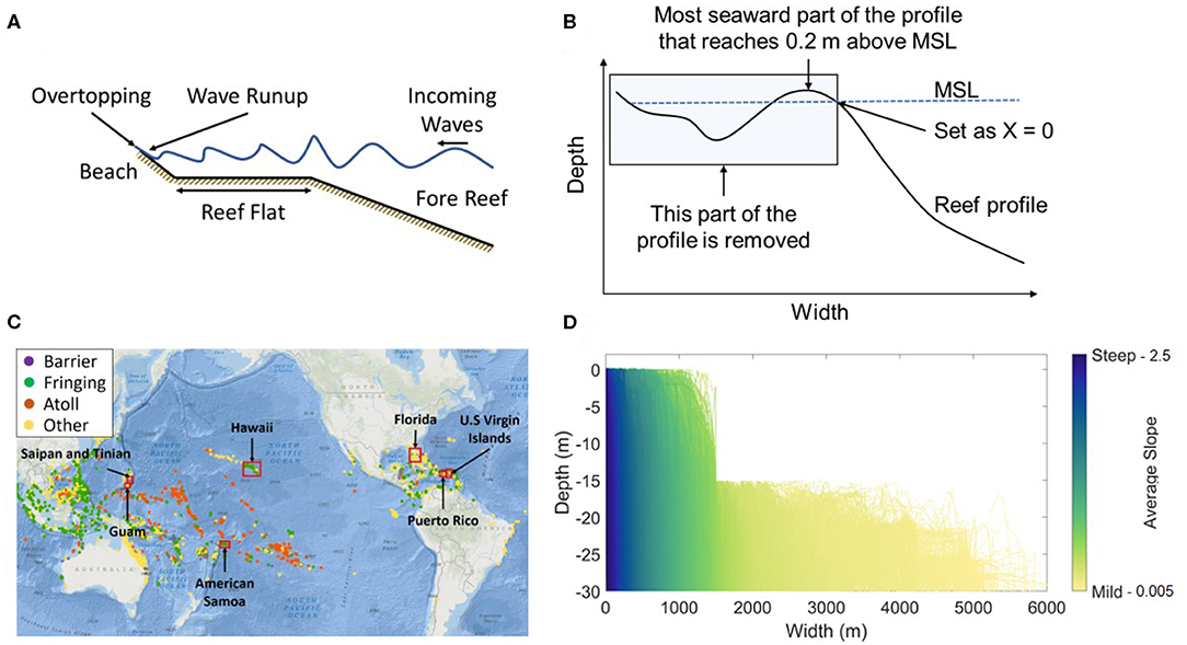
Figure 1. Coral reef profile dataset information including (A) a schematic of a typical fringing reef demonstrating wave runup and overtopping from incoming waves, (B) an example of how the reference point (X = 0) was set at MSL for aligning the cross-shore profiles, (C) a map of the locations where the coral reef topobathymetric cross-shore profiles in the dataset have been collected (ReefBase, 2019; Storlazzi et al., 2019), and (D) the selected cross-shore profiles for the study plotted and colored based on their average slope which range from 0.005 to 2.5.

Field measurements have quantified wave dynamics and wave-driven water levels on fringing coral reefs (Hardy and Young, 1996; Cheriton et al., 2016) and shown the complexity of the hydrodynamics in these systems (Storlazzi et al., 2004). The complex interaction between the reef morphology and the hydrodynamics on the reef has so far hampered the development of reliable parametric estimates of wave runup on reef-lined coasts.

In view of this complexity, numerical models are typically used to obtain estimates of wave runup at the shoreline. Numerical models can account for these hydrodynamic interactions, and can be applied to estimate extreme conditions that have never been measured, but are likely to happen or expected in a plausible future scenario (e.g., Anderson et al., 2019). Coral reef hydrodynamics have been modeled extensively (Storlazzi et al., 2011; van Dongeren et al., 2013; Buckley et al., 2014; Bosserelle et al., 2015; Lashley et al., 2018) with good predictive skill. However, each simulation of a deterministic process-based model provides only the results for the specific bathymetry included in the simulation. Coral reefs have a wide range of morphologies (Figure 1D), and each are exposed to variable hydrodynamic conditions. Therefore, the results from a single model simulation are highly location-specific, and far from being universally-applicable. Modeling each and every morphology individually, however, would be computationally extremely impractical and unnecessary since two reef profiles similar in shape would be expected to have similar hydrodynamic responses under the same hydrodynamic conditions (e.g., water level, wave, and wind characteristics), forming a set of redundant model runs. In that case, one of the reef profiles could be simulated in a model and used as an estimate of wave runup for the other.

To increase the applicability of numerical model wave runup predictions, Pearson et al. (2017) developed the “Bayesian Estimator for Wave Attack in Reef Environments” (BEWARE). BEWARE makes use of parameterized fringing coral reef profiles (beach slope, reef flat width, and fore reef slope) and hydrodynamic conditions (water depth, wave height, and wave period) to generate a synthetic database of wave runup. The database includes the results of the thousands of combinations of values for each profile parameter and offshore forcing conditions. After training the Bayesian Network (BN) with the synthetic database, it acts as an emulator or surrogate for the numerical model and provides a probabilistic estimate of wave runup for real-world coral reef profiles based on the similarity of morphology and wave conditions to that stored in the database. The database has been useful for other reanalysis studies (Pearson et al., 2018; Rueda et al., 2019b), but there are limitations that come with it. Only simplified cross-shore profiles characteristic of a fringing reef can be used (e.g., Figure 1A), and it is not representative of the global diversity of reef morphology.

This paper attempts to build upon the work of Pearson et al. (2017) by providing a methodology to account for the global variety in coral reef morphology, and their characteristic hydrodynamic response (wave runup) to offshore forcing conditions which can be used instead of the simplified cross-shore profiles in improved versions of the BEWARE model. We combine machine learning, statistics, and simulated swash dynamics using the XBeach Non Hydrostatic (XBNH) numerical model (Smit et al., 2010; McCall et al., 2014) to reduce the high diversity of coral reef topo-bathymetric profiles (>30,000) into a set of 50–312 representative cluster profiles (RCPs). We also propose a simplified approach to characterize the hydrodynamic response for any real-world coral reef cross-shore profile in terms of the simulated response of the RCPs. The methodology developed in this paper is designed to be transferable to other coastal environments, providing numerous opportunities and applications in large-scale wave runup simulation and EWSs.

Section 2 of this manuscript introduces the coral reef dataset. Section 3 describes the methodology to classify the RCPs and how to use them as a forecasting tool. Section 4 presents the results of each methodological step and of an application test case. Section 5 includes a discussion on the sensitivities of the machine learning, statistical, and numerical tools used for the development of this research, as well as the implications of the results obtained in further applications such as EWS and climate change assessment studies. Finally, we summarize the main conclusions of this research in section 6.

2. Coral Reef Dataset

The data used for this study consists of 30,166 measured coral reef topobathymetric cross-shore profiles (Storlazzi et al., 2019) from seven regions distributed through the Pacific Ocean, Atlantic Ocean, and Caribbean Sea (Figure 1C), measured between 2001 and 2016. The geographical distribution of the reef profiles is provided in Table 1.

TABLE 1

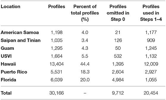
Table 1. Spatial distribution of coral reef topobathymetric cross-shore profiles included in the initial dataset, as well as the number of profiles from each location included in the study.

The profiles are aligned by taking the 0 m elevation contour with respect to mean sea level (MSL) as the shoreline reference point. Measured data points were homogenized in an uniform one-dimensional grid spaced 2 m going seaward from the shoreline. A summary of the profile dataset focusing on nearshore averaged slope geometry (computed between shoreline and 30 m depth) is presented in Figure 1D. This dataset was then filtered using procedures explained in section 3.1.

3. Development of Representative Cluster Profiles (RCPs) for Coral Reefs

To create the set of representative profiles, unsupervised cluster analysis techniques were used with the coral reef morphology and results from XBNH as inputs. The representative profiles were then tested to determine their predictive skill. The steps of the methodology are detailed in this section and are illustrated in Figure 2.

FIGURE 2

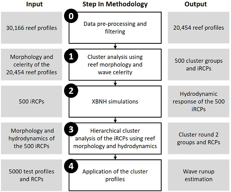
Figure 2. The methodology used to reduce the initial dataset of coral reef topobathymetric cross-shore profiles to the representative cluster profiles (RCPs). Steps 0 and 1 highlight the first data reduction step to create the 500 initial representative cluster profiles (iRCPs), Steps 2 and 3 are used to further cluster the profiles and to form the final RCPs, and Step 4 includes using the RCPs for wave runup prediction.

3.1. Step 0: Data Pre-processing and Filtering

The profiles included in the analysis were carefully selected to ensure that they resembled a reef in front of habitable land, and were not too wide so that they could accurately be modeled with XBNH. These criteria are explained in greater detail below.

Firstly, land was classified as the most seaward part of the profile with an elevation greater than or equal to 0.2 m above MSL, as detailed in Figure 1B. Low-lying coral islands have mean elevations around 2 m above present sea level (Storlazzi et al., 2018), so a value of 0.2 m is relatively low. However, if a greater threshold was used, multiple cross-shore profiles included an offshore protruding segment that was deemed unrealistic. These would have a major impact on the wave transformation over the reef and so for the purpose of this study a lower threshold of 0.2 m was used.

Secondly, the width limitation was set to ensure that all profiles included in the analysis could be accurately modeled using a one-dimensional XBNH model. Any profiles which reach -15 m depth at widths greater than 1.5 km (i.e., 10–20 wave lengths from the shoreline) were deemed too wide to accurately model, as one-dimensional XBNH models do not account for wind input, or large-scale topographic refraction. These 9,712 profiles, mostly from Florida (Table 1), were therefore removed from the dataset, resulting in 20,454 profiles to be used in Steps 1–4 of this study. The selected profiles for Steps 1–4 are shown in Figure 1D, colored based on their average slope.

3.2. Step 1: Data Reduction Using Reef Morphology and Wave Celerity

3.2.1. Cluster Analysis

To group the similar coral reef profiles and identify dominant RCPs, unsupervised machine learning was applied on the reef topobathymetric cross-shore profiles resulting from Step 0. In particular, we applied cluster analysis which is used to group a collection of objects into smaller subsets or clusters. The goal is to have the objects within each group more closely related to one another than to objects assigned to different clusters (Friedman et al., 2001). Machine learning techniques have been successfully applied for identifying patterns in different fields and processes including: waves (Antolínez et al., 2016), ocean currents (Chiri et al., 2019), sediment transport (Antolínez et al., 2018), sediment distribution (Antolínez et al., 2019), profile morphodynamics (de Queiroz et al., 2019), and atmospheric conditions (Rueda et al., 2019a).

In this study, we use the K-means algorithm (Hartigan, 1975; Hartigan and Wong, 1979) with an initialization using K-means++ (Arthur and Vassilvitskii, 2006). After exploring several different distance metrics (squared euclidean and cityblock) and statistical techniques (K-medoids, Gaussian mixture modeling, Principal Component Analysis, and Maximum Dissimilarity) (Friedman et al., 2001) the K-means clustering algorithm with the cityblock distance metric resulted in the most accurate grouping due to the profile prealignment done in Step 0. The cityblock distance metric computes the distances between observations as the sum of absolute differences, and results in each centroid being formed as the component-wise median of the observations in that cluster; therefore the method is referred to as “K-medians.”

A range (10–3,000) of initial RCPs (iRCPs) were formed using this technique to determine what may be the optimal number. This was assessed by comparing the morphological similarity of grouped topobathymetric cross-shore profiles and the required number of XBNH model runs needed for Step 2 in the methodology (Figure 3). The mean difference in morphology between a profile and its assigned centroid (iRCP) decreases significantly moving from 10 to 500 cluster groups, however beyond 500 cluster groups the gain in morphologic similarity reduces (Figure 3A) as does the added value of morphological similarity in comparison to the required number of XBNH model runs (Figure 3B), referred to here as the relative gain.

FIGURE 3

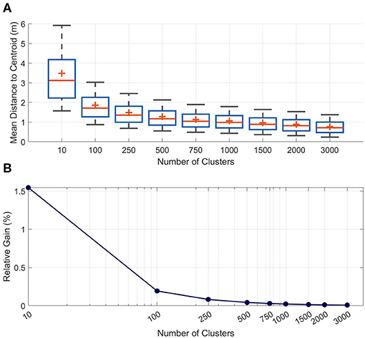
Figure 3. (A) The distribution of the mean distance between a profile and its assigned centroid (iRCP) using K-medians for the varying number of tested cluster groups. (B) The relative gain in morphologic similarity of grouped profiles compared to the required XBeach Non-Hydrostatic (XBNH) model runs. This comparison is made to a reference case of all profiles being part of one cluster group, requiring 4 XBNH model runs. The relative gain is measured as the reduction in the mean distance between profiles and their centroid, divided by the additional required XBNH model runs, normalized to provide the result as a percentage.

The relative gain is calculated as:

$\begin{array}{ll}Gain=\frac{X_0-\overline{D}}{X{B}_{runs}}& (1)\end{array}$

$\begin{array}{ll}RelativeGain(\%)=\frac{Gain}{X_0}\times 100\%& (2)\end{array}$

Where X₀ is the mean distance between all profiles and their centroid for the case of all profiles being placed in one cluster group [units (m)], $\overline{D}$ is the mean distance between all profiles and their respective centroid [units (m)], and XB_runs is the number of required XBNH model runs [units (-)]. The Relative Gain (%) is then a measure of how well the clustering has increased the morphologic similarity of the grouped profiles, weighted against the number of required XBNH model runs. Using these two metrics, 500 iRCPs was determined to be the ideal combination of intra-cluster similarity and high data reduction.

3.2.2. Cluster Analysis Inputs

The initial cluster analysis was performed using the water depth and computed wave celerity as inputs (Figure 4). Whereas, water depth has previously been used to define cross-shore profile clusters (Cohn and Ruggiero, 2016; Costa et al., 2016; Duce et al., 2016), wave celerity was included in this study to provide greater specificity between profiles in shallower depths. Wave celerity is more sensitive to changes in water depth in shallow water than in deep water, so its inverse was used as a non-linear weighting component in the clustering algorithm, with higher weight given to depth similarity in shallow areas (Figure 4C).

FIGURE 4

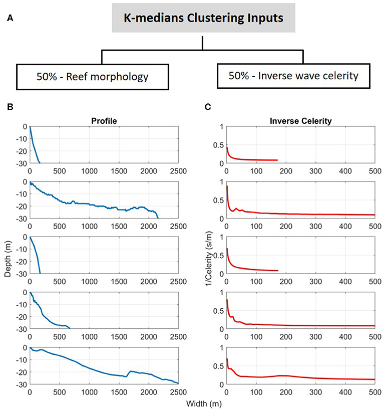
Figure 4. The inputs used for the K-medians algorithm, (A) highlighting the weighting assigned to the two inputs; reef morphology and inverse wave celerity. (B,C) Examples of these two inputs for 5 topobathymetric cross-shore profiles.

Using a wave period of 8 s, the celerity was computed using linear wave theory at each cross-shore position in order to obtain an equivalent dataset to the cross-shore depths. An 8 s period was used as a representative value for waves reaching coral reef lined coasts, although the specific value is not crucial for this application. This is because in shallow water the celerity for all realistic wave periods tends to $\sqrt{gh}$, providing the desired effect.

A value of infinity is reached for the inverse celerity at depths of 0 or above MSL. For these points, the inverse celerity was set to 0. The goal is that profiles with similar characteristics are grouped together; assigning the same value for these instances guides profiles with similar characteristics to be grouped in the cluster analysis. The depths and inverse celebrities were then combined into one matrix to be used for the cluster analysis by normalizing the values using max-min scaling. The morphology and inverse celerity received equal weighting (Figure 4A).

3.3. Step 2: XBNH Simulations

XBNH is a process-based numerical wave and water level model. It includes a non-hydrostatic pressure correction term that allows wave-by-wave modeling of the surface elevation and depth-averaged flow (McCall et al., 2014). This model has similar accuracy to that of lower order Boussinesq models and has commonly been used since its development for wave modeling over coral reefs (Quataert et al., 2015; Pearson et al., 2017; Lashley et al., 2018; Klaver et al., 2019; Rueda et al., 2019b).

We applied four wave conditions to each of the 500 iRCPs using XBNH. The objective was to obtain hydrodynamic responses for each profile to be used as a proxy for a further data reduction. The wave conditions used for the simulations are shown in Table 2. Two wave heights and wave steepnesses were selected with constant water level, reef friction, and beach slope to generate the four conditions. The wave height and steepness values were selected to represent typical wind wave and swell events that any of these regions could experience and could cause flooding. They were also chosen to vary considerably to ensure profiles are grouped which experience similar hydrodynamics from a wide range of conditions, not just one event. A dimensionless coefficient of friction (c_f) of 0.05 was used for the reef profile below MSL per Pearson et al. (2017), and a coefficient of friction of 0.01 was used for the beach (above MSL). To compute the wave runup potential, a semi-infinite beach slope was required. This was implemented using a beach slope of 1/10 from the shoreline position, reaching an elevation of 30 m above MSL.

TABLE 2

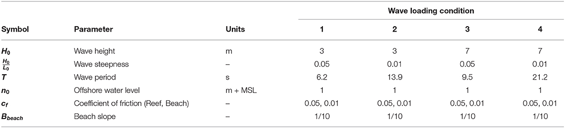
Table 2. XBeach model wave loading conditions and additional reef profile parameters.

XBNH was applied in one-dimensional mode which does not account for some of the dynamics that occur on natural reefs. However, the dataset consists of one-dimensional profiles, and extrapolating them to an unknown two-dimensional bathymetry would involve many unwarranted assumptions, as well as a steep increase in computational time. One-dimensional analysis on coral reefs has been done for many applications, and the choice for our methods builds on existing observations along 1D transects in the field (Péquignet et al., 2011; Becker et al., 2014; Cheriton et al., 2016) and laboratory environments (Massel and Gourlay, 2000; Nwogu and Demirbilek, 2010; Buckley et al., 2016), as well as many 1D numerical modeling studies (Yao et al., 2012; Quataert et al., 2015; Pearson et al., 2017; Beetham and Kench, 2018). Furthermore, the one-dimensional modeling will represent a conservative estimate for wave runup, as the forcing is shore-normal (Guza and Feddersen, 2012; Quataert et al., 2015).

3.4. Step 3: Data Reduction Using Hydrodynamic Response

In an effort to further reduce the dataset, the 500 iRCPs were grouped based on their hydrodynamic response in the XBNH simulations. Since the objective of the RCPs is to forecast wave run-up, if there are two or more profiles of the 500 iRCPs which experience very similar wave run-up characteristics for all wave conditions, they essentially form a redundant group and can all be represented by one of the profiles. Agglomerative hierarchical clustering (Day and Edelsbrunner, 1984) was used to find which of the 500 iRCPs should be grouped together.

3.4.1. Cluster Analysis Inputs

The variables used for this stage of data reduction include both the reef morphology and hydrodynamic response; each with 50% weighting (Figure 5A). Morphology is included again to account for the fact that only four wave conditions were tested in XBNH. These are insufficient data to guarantee similar wave runup results across the full range of potential hydrodynamic conditions. Including morphology reduces this uncertainty. The hydrodynamics include the R_2%, setup at the shoreline, and swash separated into infragravity and sea-swell components. The R_2% was calculated by isolating all wave runup events and distinguishing the 2% exceedance value. The setup was calculated as the mean water level at the shoreline over the duration of the XBNH model run. Lastly, the swash was calculated by first generating the spectrum of the water level timeseries at the shoreline. The spectrum was then split into infragravity and sea-swell components at a frequency of 0.05 Hz (period = 20 s) (Herbers et al., 1995) and the two swash values were calculated from the spectral energy using trapezoidal numerical integration (Stockdon et al., 2006). The 50% weighting is divided equally among the three hydrodynamic components.

FIGURE 5

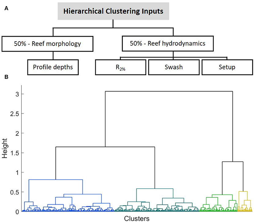
Figure 5. The inputs used for the hierarchical clustering algorithm, (A) highlighting the weighting assigned to the inputs; morphology and hydrodynamics separated into R_2%, setup and swash. (B) The dendrogram used to visualize the hierarchical clustering results of the 500 initial representative cluster profiles (iRCPs). The coloring represents an example of the grouping of the 500 iRCPs if a height cutoff value of 1 is used, forming four clusters.

3.4.2. Agglomerative Hierarchical Clustering

Agglomerative hierarchical clustering builds a hierarchy from the individual observations (in this case, iRCPs) by progressively merging clusters which have the smallest inter-group dissimilarity (Madhulatha, 2012). A dendrogram is typically used to visualize hierarchical clustering (Figure 5B). The lowest level of the hierarchy includes all of the iRCPs treated as individual clusters, and at the highest level all iRCPs are grouped together into one cluster. This method stops grouping when a threshold of dissimilarity is reached. Therefore, varying thresholds and measures of dissimilarity will result in different final numbers of RCPs. For this study, the inconsistency coefficient was used as the measure of dissimilarity (Zahn, 1971; Jain and Dubes, 1988) which compares the height of each link with the average height of other links at the same level. Using values of 0.68, 0.72, 1.1, 1.14, and 1.54, final groups of 312, 201, 149, 109, and 50 RCPs of varying sizes were generated and compared for this study.

One of the iRCPs from each group formed during the hierarchical clustering process was selected to be the representative cluster profile (RCP). This profile was the closest to the mean in terms of R_2%. If there are two iRCPs in the final group, they would both be equal distance from the mean; in that case the iRCP which represents the greater number of profiles from the first round of cluster analysis was selected as the RCP.

3.5. Step 4: Application of Representative Cluster Profiles

The prediction of the RCPs can be evaluated by comparing the wave runup estimate generated from the RCPs to the modeled wave runup from a set of test topobathymetric cross-shore profiles. To do so, 5000 test profiles were randomly taken from the post-Step 0 dataset after sorting them by average slope to ensure that the shapes of the test profiles were sufficiently varied. Each of these profiles were simulated in XBNH under the same four wave loading conditions that were used for the iRCPs in Step 2.

3.5.1. Matching Test Profiles to Representative Cluster Profiles

Two methods were used to match the test profiles to their corresponding RCPs: a direct match to the RCPs, and a probabilistic matching technique. For both cases, test profiles are first matched to the 500 iRCPs of Step 1, and the relationship is followed between iRCP to RCP (Step 3) to determine the appropriate RCP match. This is done because the match is based on the profile morphology and inverse celerity, and therefore the match must be made to the iRCPs that were formed based on those same parameters.

The direct match is simply done by calculating the pairwise distance between the test profile and 500 iRCPs. The distance is a sum of the distance between the normalized depths and celerity; the same variables used in the first cluster analysis. The match is made to the iRCP with the smallest distance and then to the corresponding RCP.

The probabilistic matching method revolves around the softmax function which is a method used in neural networks to predict the probabilities associated with a multinoulli distribution (Goodfellow et al., 2016). It maps a vector of inputs to a posterior probability distribution (Goodfellow et al., 2016). Once the distances have been calculated between a test profile and all iRCPs, if the distances are input into the softmax function, each distance is attributed a probability ranging between 0 and 1.

The softmax function is defined as:

$\begin{array}{ll}S{(x)}_i=\frac{exp(-B*x_i)}{{\displaystyle {\sum }_{j=1}^n}exp(-B*x_j)}& (3)\end{array}$

where S(x) is the probability of matching to iRCP i, x_i is the distance between the test profile and iRCP i, x_j is the distance between the test profile and iRCP j, B is the stiffness parameter, and n is the number of iRCPs.

The B value essentially acts as an inverse variance, such that larger values of B will cause the distribution to be narrower so that probabilities associated to large distances between profiles will become small. Multiple B values were tested to compare the effect on the accuracy of the R_2% estimate.

The steps of the probabilistic matching technique are listed below:

1. Calculate the distance between the test profile and the 500 iRCPs.

2. Use the softmax function to transform the distances into probabilities. A lesser distance will lead to a greater match probability.

3. Determine the match probability to the RCPs by summing the probabilities of the grouped iRCPs.

4. Use the probabilities as weights and generate the estimate of the wave runup as an ensemble average.

3.5.2. Performance Metrics

The accuracy of the RCP prediction of R_2% was assessed using common performance metrics including the root mean square error (RMSE), coefficient of determination (R²), bias, skill and scatter index (SI). RMSE is a measure of how concentrated the data is around the line of best fit. If all data points lie on the line of best fit, the RMSE is 0. R² is a measure of the variance in the dependent variable (modeled value) that is predictable from the independent variable (RCP estimation). Bias is the tendency of the RCP estimate to either over or underestimate the modeled value. The skill score (Murphy, 1988) is a measure of accuracy of prediction, where a value of 1 indicates a perfect prediction. The scatter index is the RMSE normalized by the mean observed value, which provides insights on the variance of the errors.

These metrics are defined as:

$\begin{array}{ll}RMSE=\sqrt{\frac{1}{n}{\Sigma }_{i=1}^n{(R_{2\%T{P}_i}-R_{2\%RC{P}_i})}^2}& (4)\end{array}$

$\begin{array}{ll}Bias=\overline{R_{2\%RCP}}-\overline{R_{2\%TP}}& (5)\end{array}$

$\begin{array}{ll}{R}^2=\frac{1}{n}{\displaystyle \sum _{i=1}^n}{(R_{2\%RC{P}_i}-R_{2\%T{P}_i})}^2& (6)\end{array}$

$\begin{array}{ll}Skill=1-\frac{RMS{E}^2}{{\sigma }_{R_{2\%TP}}^2}& (7)\end{array}$

$\begin{array}{ll}SI=\frac{RMSE}{\overline{R_{2\%TP}}}& (8)\end{array}$

where R_2%RCP is the forecasted R_2% from the RCPs, R_2%TP is the modeled R_2% of the test profile, σ_R2%TP is the standard deviation of the modeled R_2% of the test profiles and n is the number of test profiles.

4. Results

4.1. Step 1: Cluster Round 1

The first cluster analysis organized the 20,454 profiles resulting from Step 0 into 500 groups. The median of each group is used as the representative profile and is known as the iRCP. The 500 iRCPs are shown in Figure S1. An example of ten cluster groups is shown in Figure 6, illustrating the range in morphologies within the groups using the 95th and 5th percentile as bounds, and the standard deviation. The cluster analysis groups profiles with similar shape and with lesser variance in shallower depths.

FIGURE 6

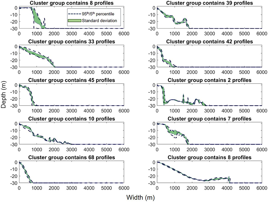
Figure 6. Example of 10 cluster groups used to form the initial representative cluster profiles (iRCPs). The x-axis represents the cross-shore width and the y-axis the elevation. The green area defines the standard deviation within the cluster and the blue dashed lines the 5th and 95th percentiles. The number of reef topobathymetric cross-shore profiles within the cluster is shown in the title of each subplot.

4.2. Step 2: XBNH Simulations

The XBNH simulations with the 500 iRCPs were mainly used to generate input for the data reduction in Step 3, however it is also interesting to analyze the range of hydrodynamic results across such a variety of coral reef morphologies.

In general, there is a greater variance in the hydrodynamics for the 500 iRCPs under the more severe loading conditions (Figure 7). Loading condition 4, which includes a 7 m significant wave height and 21 s period, has the greatest range of R_2% and setup, whereas loading condition 1 with a 3 m significant wave height and 6 s period has the narrowest range of results for these parameters (Figures 7A,B). Both the infragravity and sea-swell swash are typically greater for the wave conditions with the higher period (lesser steepness) (Figures 7C,D).

FIGURE 7

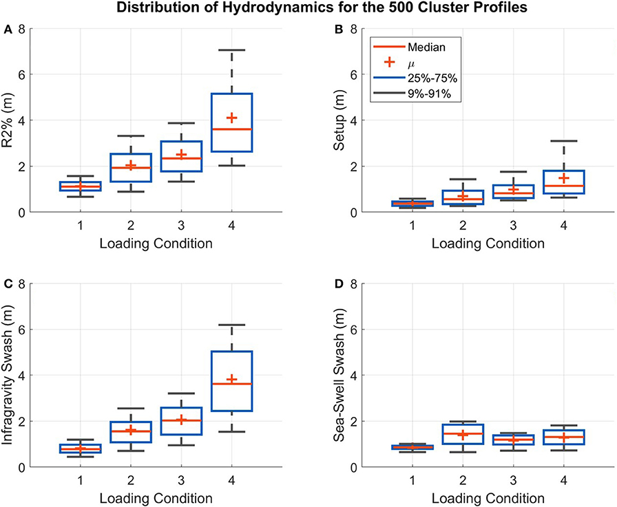
Figure 7. Distributions of the results of the XBeach Non-Hydrostatic (XBNH) runs for the 500 initial representative cluster profiles (iRCPs), including the R_2% (A), setup at the shoreline (B), infragravity (C), and sea-swell swash (D). The loading condition numbers along the x-axis correspond to the numbering in Table 2.

4.3. Step 3: Cluster Round 2

The second round of data reduction grouped the 500 iRCPs by morphology and hydrodynamics. Five different thresholds were used to limit the dissimilarity of joined observations, as explained in section 3.4.2, resulting in different numbers of final RCPs. The five thresholds resulted in 312, 201, 149, 109, and 50 RCPs.

To assess the success of Step 3, the intra-cluster similarity of the XBNH results was compared. This was done by measuring the relative difference of the relevant hydrodynamic parameters between grouped iRCPs. XBNH results are only available for the 500 iRCPs and so the analysis was done with these results, however the 500 iRCPs represent the original 20,454 profiles included in the study, and therefore this step provides a measure of how similar the hydrodynamics are for all the profiles grouped through the two cluster analyses. The R_2%, setup at the shoreline, and swash separated into infragravity and sea-swell components were compared. As expected, the relative difference increases when there are fewer cluster groups because more profiles with varying hydrodynamic results are being grouped together (Figure 8A). This leads to the conclusion that the accuracy of the hydrodynamic prediction using the RCPs will be greater when more RCPs are included.

FIGURE 8

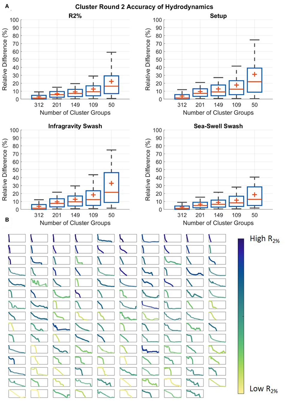
Figure 8. (A) The similarity of the R_2% (top left), setup at the shoreline (top right), infragravity (bottom left), and sea-swell swash (bottom right) of the grouped initial representative cluster profiles (iRCPs) from the hierarchical cluster analysis (Step 3). The x-axis contains the number of representative cluster profiles (RCPs), and the y-axis is the relative difference in the XBeach Non-Hydrostatic (XBNH) model results between all grouped profiles and their representative profiles. The grouped profiles are the iRCPs from Step 1, and the representative profiles are the RCPs formed in Step 3. (B) The RCPs for the case of 149 cluster groups, colored based on their relative wave runup rank, and sorted based on their average slope from 0 to 15 m depth. The x-axis is the profile width set at a constant range of 0 to 3,068 m, and the y-axis is the profile depth from MSL set at a constant range of −30 to 0 m.

The general relationship, which matches previous research (Storlazzi et al., 2011; Quataert et al., 2015; Pearson et al., 2017), is that reefs with wide flats, shallow average depths and mild fore-reef slopes result in the lowest wave runup, whereas reefs with very narrow reef flats, greater average depths, and steeper foreshores result in the highest wave runup (Figure 8B). This supports the inverse celerity weighting to decipher between the different profiles.

4.4. Step 4: Application of the Representative Cluster Profiles

The forecast of the RCPs was tested with 5000 profiles from the dataset. As mentioned in section 3.5.1, two methods to match the test profiles to the cluster profiles were assessed.

4.4.1. Probabilistic Match

Using the probabilistic matching method, the most accurate estimate of R_2% was obtained with the highest B value (Figure 9A). When comparing the estimated R_2% from the RCPs to the model results, a B of 1,200 resulted in a mean relative difference between 9.7 and 13.1% depending on the number of RCPs, ranging from 312 to 50. In contrast, a B value of 100 results in the mean relative difference always being greater than 20%. Referring to the example test profile in Figure 9B, when B = 100, no RCP is given a match probability greater than 10% and many are given a probability above 0.1%, whereas when B = 1,200, two RCPs are assigned the majority of the probability at about 40% each and few others carry any probability at all. The general trend is that as B increases the association to the closest RCP increases and the estimate becomes more accurate (Figures 9A,B), although this is not the case for all profiles.

FIGURE 9

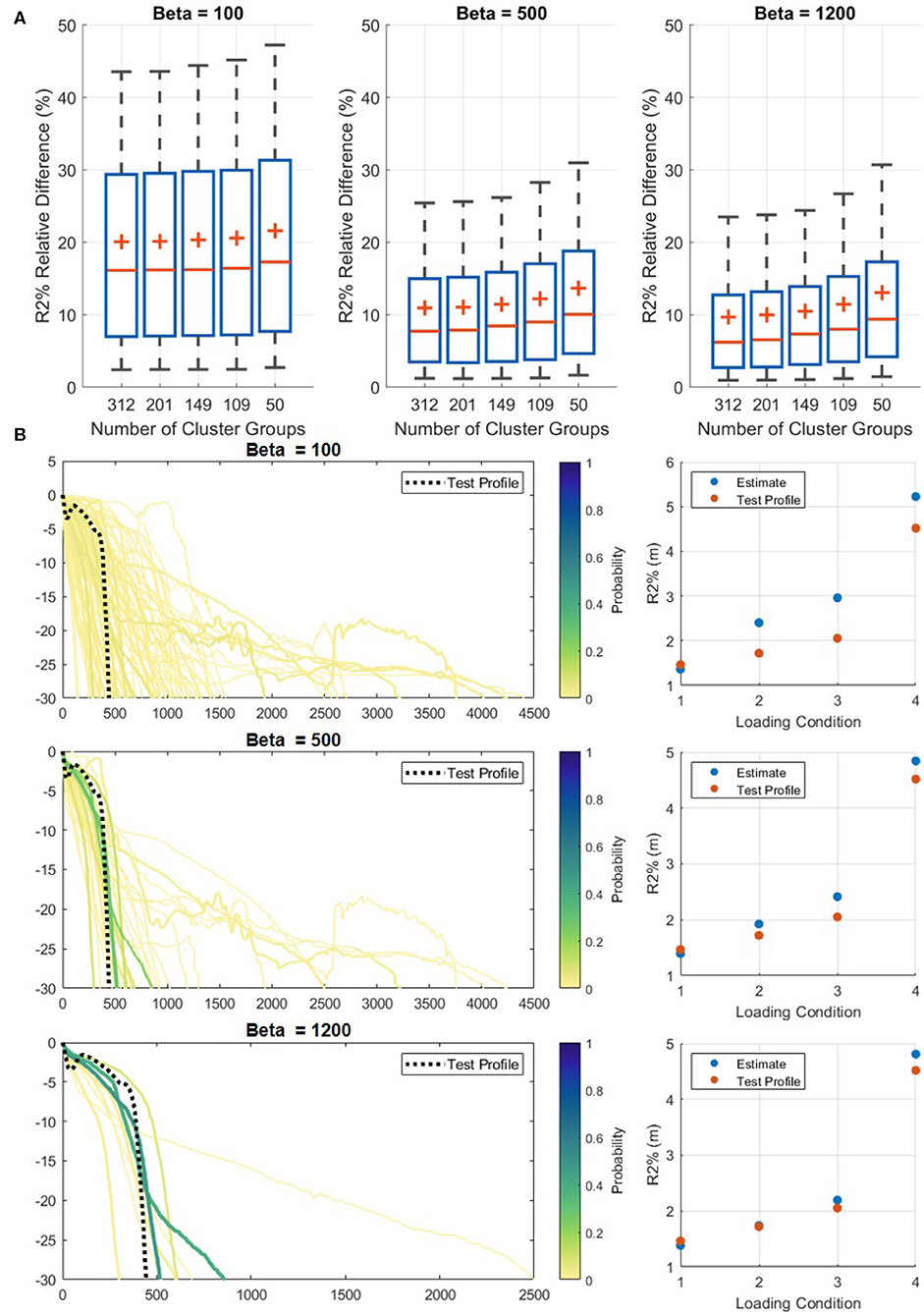
Figure 9. Results of the influence of the B value in the probabilistic matching method. (A) For increasing values of B and representative cluster profiles (RCPs), the accuracy of the R_2% estimation increases. (B) An example of matching the RCPs with one real-world test profile for varying values of B. As B increases, the match to the most similar RCP increases and fewer RCPs are given any match probability. RCPs are only plotted if they have a match probability above 0.1%. The scatter plots provide the modeled value and estimate of R_2% for the four loading conditions (Table 2).

The B value was capped at 1,200 since this was deemed to be the upper limit for the softmax function to operate properly with the current inputs. There is not an optimized value of B for the softmax function applied in this study since the range of applicable B values is dependent on the input x_i and x_j from Equation (3). For the values used in this study, it was found that B values >1,200 resulted in function errors.

4.4.2. Probabilistic vs. Direct Match

While using the probabilistic method, the estimation is most accurate when the association to one RCP is greatest. However, a direct match to the single most similar RCP generally does not result in a greater accuracy. The comparison of the probabilistic matching method using the high B value of 1,200 compared to the direct matching method is shown in Figure 10A. For the 5,000 test profiles, the direct matching technique results in slightly greater error in the R_2% estimates.

FIGURE 10

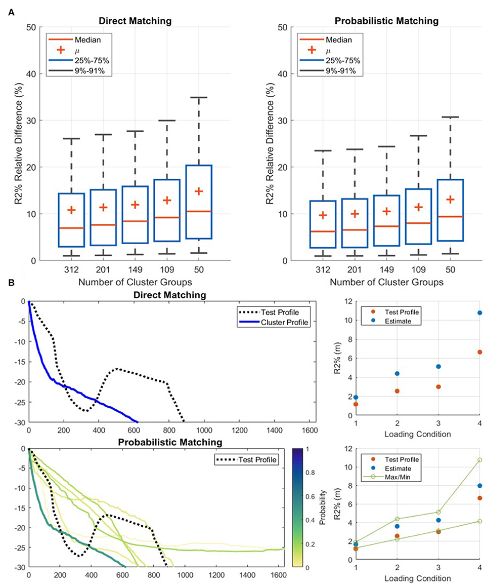
Figure 10. Results of the direct and probabilistic matching method. (A) The probabilistic technique has a slightly greater accuracy in R_2% estimation. For both cases, the accuracy decreases as the number of representative cluster profiles (RCPs) decrease. (B) An example of the two matching techniques when using 50 RCPs with one of the unique test profiles. The scatter plots provide the modeled value and estimate of R_2% for the four loading conditions (Table 2). The test profile does not match well to any of the RCPs, and therefore the R_2% estimation from the direct matching technique suffers. The estimation from the probabilistic technique is influenced from multiple RCPs and is more accurate for all four loading conditions. The green values in the scatter plot represent the confidence bands that can be determined while using the probabilistic technique.

The results from the two matching techniques differ the most at the lowest number of RCPs (50). Here, the probabilistic method offers the greatest benefit. If a profile is not very similar to any RCPs, which is more common when there are fewer RCPs to match to, the probabilistic method is able to draw an estimate as an average of the most similar RCPs, most likely combining over and under estimated values. Conversely, for the direct match method the best estimate is one of the over or under estimated values. An example of this is shown in Figure 10B where the test profile does not match well to any RCP and the direct matching method therefore provides inaccurate R_2% estimates. The estimates increase in accuracy under the probabilistic matching method where the R_2% value is derived from multiple RCPs instead.

An added benefit of the probabilistic method is that confidence bands can be added to the R_2% estimate (Figure 10B). To cover the full range of potential outcomes, all RCPs with a match above 1% can be used to create a confidence band to aid the prediction, which when matching to a single RCP cannot be provided.

4.4.3. Cluster Profiles Predictive Skill

The predictive skill of the RCPs while using the probabilistic matching method for the 5,000 test profiles is shown in Figure 11. There is a strong linear relationship for the case of 312 RCPs, meaning that the majority of the data points have <10% deviation between predicted and modeled values, which gradually reduces moving toward 50 RCPs. For all RCP values, the majority of instances when the error is >10% occur at lower R_2% values, meaning that the estimate is typically more accurate for predicting flood scenarios (high R_2%) compared to more mild conditions.

FIGURE 11

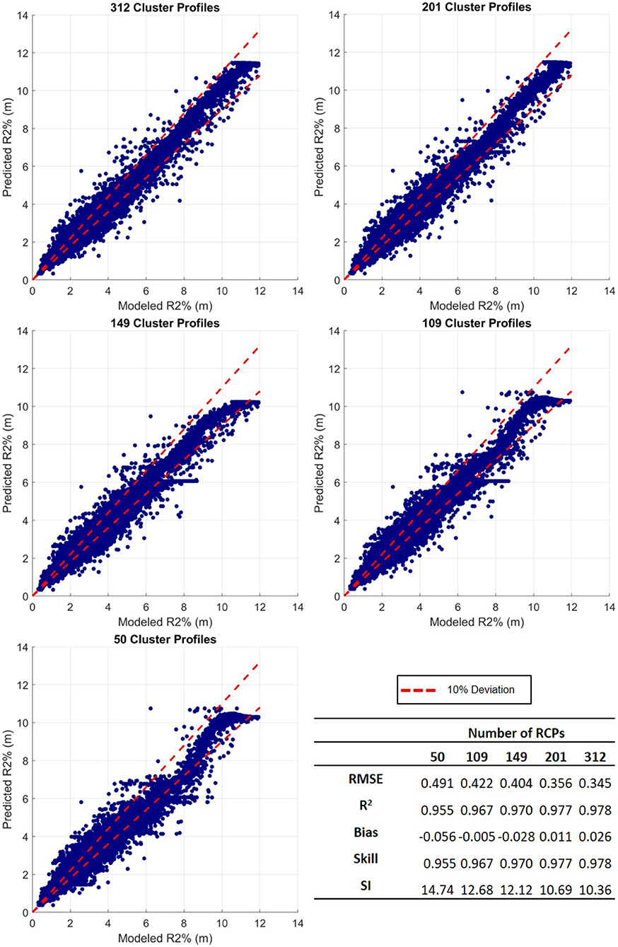
Figure 11. Modeled vs. estimated R_2% for the five different numbers of representative cluster profiles (RCPs), ranging from 312 (top left) to 50 (bottom left). The table in the bottom right provides data comparison statistics, explained in section 3.5.2.

All performance metrics, explained in section 3.5.2, lead to similar findings. The RMSE continuously decreases for greater numbers of RCPs, meaning that the data is most concentrated around the line of best fit with more RCPs. The increasing R² and skill, as well as the decreasing SI all suggest that the predictability is enhanced as more RCPs are used. Finally, the bias switches between positive and negative suggesting either over or underestimating, however in all cases it is relatively low.

These results suggest that the RCPs are highly effective in predicting the R_2% for the 5,000 test profiles considered for this study. When using 312 RCPs the accuracy is greatest, forecasting the R_2% with a mean relative difference of 9.7%. Fewer RCPs can be used, however, increased data reduction comes at the expense of higher predictive error. Using 50 RCPs (fewest tested) results in a mean relative difference of 13.1%. These error values are within the same range as the empirical equation developed by Stockdon et al. (2006) to calculate R_2% for natural beaches, used by engineers around the world.

5. Discussion

The presented methods and techniques have not been widely used for applications in coastal engineering. This section provides the main sensitivities and potential future applications of this work.

5.1. Cluster Analysis

Two cluster analyses were performed to develop the RCPs of the dataset. The techniques to generate these RCPs can vary significantly, and although the presented methods were selected in order to create the optimal RCPs, modifications could be made which would alter the outcome. The key sensitivities of the cluster analysis include the cluster method, the variables, and the weighting of the variables.

Many cluster analysis techniques are applicable for this type of study, and each has pros and cons (Friedman et al., 2001; Rai and Singh, 2010). Other methods have also been applied and compared in other coastal engineering applications (Camus et al., 2011). For this dataset, K-medians was determined to result in the least intra-cluster variance of morphology compared to K-means, K-medoids, Maximum Dissimilarity, and Principal Component Analysis. However, other benefits may come from using one of the other methods which has not been explored. Hierarchical clustering was selected for the second cluster analysis because it works well with varying attribute types or large datasets, and a threshold can be set to limit the intra-cluster dissimilarity (Madhulatha, 2012).

Apart from the clustering technique itself, the input into the algorithm is equally important. In the first cluster analysis, the normalized bathymetric profile depths and inverse wave celerity were used (Figure 4) to group similarly shaped profiles with an emphasis on the shallower part of the profile. This selection is appropriate for the goal of this study, however other parameters could be used as well. The celerity does not account for the impact of the slope of the fore reef, which is known to impact the infragravity components of the incoming waves (Storlazzi et al., 2011; Quataert et al., 2015; Pearson et al., 2017). Using celerity therefore excludes a potentially key aspect of successful grouping. In the second cluster analysis, the topobathymetric cross-shore profile was combined with the hydrodynamic response at the shoreline determined from the XBNH simulations for the input into the clustering algorithm. These were selected to group profiles with the most similar flooding characteristics, but again, other parameters may be used. For example, the infragravity and sea-swell components of the wave height at a certain distance offshore may be beneficial to add as an input, however by using the R_2%, setup, and swash separated into infragravity and sea-swell components, most of the important information is already included.

Lastly, the weighting of the inputs can be modified to vary the relative importance of certain inputs. In the first cluster analysis, the inverse wave celerity was included as a weighting function. This is because the wide variety of coral reef morphologies makes it difficult to apply a simple weighting function that can be used across all topobathymetric cross-shore profiles. Since the required weighting is proportionate to the depths (values), not the cross-shore position (variables), the weight for the same variable (cross-shore position) would not be consistent across all profiles. Therefore, the inverse wave celerity was selected which includes the influence of the shallow depths of the profile. For both the first and second cluster analysis, 50% weighting was applied to the morphology and 50% to the celerity or hydrodynamics. An equal balance was selected because the relative contribution of the inputs to the successful clustering based on wave runup is not certain. It would be interesting to compare the RCPs with different weighting assigned to the morphology and hydrodynamics, for example if 100% weighting was assigned to the hydrodynamics. Most likely the results would not be influenced heavily because the morphology also characterizes the hydrodynamic response.

5.2. Wave Conditions

The results from the XBNH simulations are a driving factor for the final grouping of the iRCPs. In this study, four wave conditions were used (Table 2) that ranged in period from 6 to 21 s, and in height from 3 to 7 m. Although they were chosen strategically to cover a wide range of potential flooding conditions and different types of ocean waves, if two profiles have similar wave runup over these four conditions, it does not necessarily mean that they always will for higher or lower energy conditions. The cluster analysis and accuracy of RCP's prediction are therefore limited by the variety of tested wave conditions.

5.3. Estimating Wave Runup

Two methods for using the RCPs to estimate the wave runup were developed. The probabilistic approach has proven to typically have a greater accuracy in the R_2% prediction compared to the direct matching method and comes with the added benefit of a confidence band associated with the estimate (Figure 10). Other matching techniques could be developed and tested, however the idea of using probabilities associated with the prediction is beneficial if considering implementing the RCPs with a Bayesian Network (BN) or other probabilistic tool. BNs are probabilistic models that have been successfully used to make predictions of hydrodynamics and morphology in numerous coastal applications (Gutierrez et al., 2011, 2015; Plant and Holland, 2011; Poelhekke et al., 2016). After being trained with sufficient data, they rely on Bayesian probability to make predictions of desired output. In this case, the input would be the profile and offshore wave conditions, and the output would be the wave runup and other hydrodynamic results. The results of the probabilistic matching could also be fed into the network to aid the prediction.

To further validate the results, the RCPs should be used to estimate the wave runup of coral reef profiles that were not included in the initial dataset. Since the 5,000 test profiles were included in the generation of the RCPs, at least one of the RCPs should be similar in shape and wave runup to each of the test profiles. For other cross-shore profiles with morphology within the range of the profiles included in this study, the accuracy of the wave runup estimation should not vary significantly.

To include a new batch of coral reef profiles, the methodology would have to be repeated. This would require going back to Step 0 to filter and align the profiles before performing the first cluster analysis. An update would only be beneficial if the new profiles are significantly different to any of the 500 iRCPs presented in this study; only then would a new cluster group be created. Otherwise, the new profiles would join one of the existing cluster groups and the outcome would not have a significant change.

5.4. Application of the Methodology

The presented methodology has been demonstrated with many coral reef properties set as constant. It is well-established that changes in the roughness and friction (Lowe et al., 2005; Pomeroy et al., 2012; Monismith et al., 2015; Buckley et al., 2016; Rogers et al., 2017, 2018; Osorio-Cano et al., 2019; Reguero et al., 2019), porosity (Lowe et al., 2008; Asher et al., 2016; Asher and Shavit, 2019; Zhu et al., 2019), and storm surge (Hoeke et al., 2013; Smithers and Hoeke, 2014; Tajima et al., 2016) will affect the hydrodynamics over a coral reef, and in turn the resulting wave runup at the shoreline. Therefore, the RCPs as they are currently do provide a means to estimate wave runup based on reef morphology, although the estimate is limited to coral reefs with similar properties used in this study. The effects of the reef properties were excluded from the scope of this study because the information for this dataset is not available. Although the properties are not included, we were able to distinguish the representative profile shapes which can be used to form the foundation for an effective tool that does encompass the full range of effects that physical reef properties have on the hydrodynamics.

As mentioned in section 1, this study was conducted to continue the work of Pearson et al. (2017), and the intended use of the RCPs is to replace the simplified profiles used in developing a predictive model such as BEWARE. Combining the RCPs with such a model would be a step toward the development of a global flood EWS for coral-reef lined coasts. To do so, similar steps done by Pearson et al. (2017) would have to be followed, including training the model with XBNH results that incorporate the variation in reef properties, such as performing multiple simulations for the same reef profile but with varying values of friction. Each of these combinations is then also required to be simulated under a range of wave conditions. This way, the model includes the combination of the full range of reef morphologies, physical properties, and offshore forcing conditions, which also allows the user to estimate wave runup based on these specifics.

One of the benefits of using the RCPs compared to a simplified reef profile (e.g., Pearson et al., 2017) is that when a greater variety of reef morphologies are included (more cluster profiles), the number of required XBNH runs increases linearly. For a simplified reef profile defined by parameters (e.g., fore reef slope, reef flat width, reef crest height), additional parameters must be included to expand the variety in morphology that they can represent (e.g., Figures 12A,B where an irregularity along the reef flat is added). Each additional parameter exponentially increases the number of combinations of profile shapes, and in turn exponentially increases the number of required XBNH runs, as shown in Figure 12. Therefore, the RCPs heavily reduce the computational time required to create a probabilistic model.

FIGURE 12

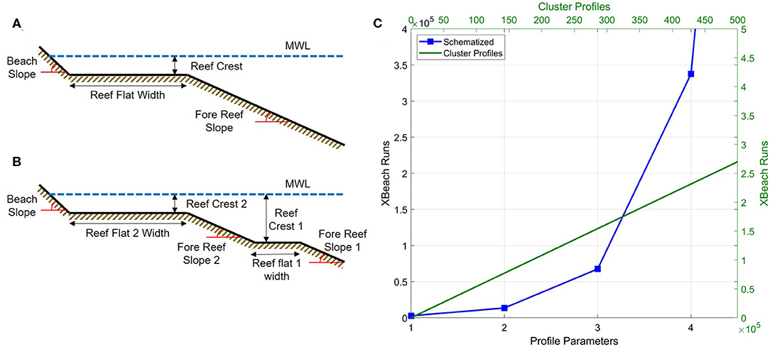
Figure 12. The required number of XBeach Non-Hydrostatic (XBNH) runs (C) for different numbers of representative cluster profiles (RCPs) (top and right axis) or a schematized profile (bottom and left axis) such as that of BEWARE, assuming 540 XBNH runs are needed per profile (Pearson et al., 2017). (A) An example of a schematized profile with four parameters and (B) how three more parameters are required to be added to the schematized profile in order to represent a second reef flat, corresponding to the x-axis in (C).

Apart from wave runup estimation, another use for the RCPs within a probabilistic model is estimating future impacts based on climate change scenarios. Since the model is a quick and accurate tool, many different loading conditions with varying offshore water levels and wave parameters could be analyzed to estimate the associated flooding impacts that they would cause. Since the RCPs encapsulate such a wide variety of real-world topobathymetric profiles, large-scale climate change estimates could be made to assess the effects of different rates of SLR on multiple different coral reef profiles, providing valuable information about the types of coastlines and their associated communities and infrastructure that are most at risk.

A comparison between the estimated wave runup from the RCPs and BEWARE with measured wave runup has not been done. It is difficult to source valid field measurements of wave runup, and they are typically recorded at time intervals much greater than what is modeled, as well as at varying vertical levels which make the comparison challenging. The assumption is that the RCPs would enhance the predictive accuracy, especially for the obscure reef profiles, most dissimilar to the schematic fringing reef used in BEWARE.

6. Conclusions

Data mining techniques were used to reduce an extensive dataset of coral reef topobathymetric cross-shore profiles to a subset of RCPs. We carried out two stages of cluster analysis that grouped the profiles based on morphology, inverse wave celerity, and hydrodynamic response to typical storm wave conditions. Techniques developed here can be used to effectively match real-world coral reef cross-shore profiles to the RCPs in order to generate an estimate of wave runup.

The RCPs have demonstrated a high predictive skill for the R_2%, used to indicate extreme wave runup and potential flooding. The accuracy of projections is in the same range as the empirical equation of R_2% for natural beaches (Stockdon et al., 2006) that is used by engineers around the world. A useful next step would be to incorporate the RCPs into a BN or other probabilistic model, developed to also accommodate the ranges in physical reef properties such as friction which have been omitted from this study. Such a model would be able to provide accurate estimates of wave runup for an extensive array of coral reefs and offshore wave conditions, and could form the basis of an EWS and scenario assessment tool for reef-lined coasts.

Data Availability Statement

All coral reef profiles used in this study, as well as the XBNH results for the 500 iRCPs is available as a NetCDF (*.nc) file at the following location: https://doi.org/10.5066/P9C39WNE.

Author's Note

Any use of trade, firm, or product names is for descriptive purposes only and does not imply endorsement by the U.S. Government.

Author Contributions

FS has been the main author of this research, first working on this topic during his thesis at Deltares/TU Delft, and continuing while working at Baird & Associates. RM and JA were the daily supervisors, offering guidance and ideas throughout the entire process. AR, CS, and SP were also all supervisors, involved in monthly meetings to provide insights and guidance. The work largely built off of previous work done by SP, and many of the coding applications can be attributed to him.

Funding

This material was based upon work supported by the U.S. Geological Survey under Grant/Cooperative Agreement No. G20AC00009. Funding was made available through the Deltares Quantifying flood hazards and impacts (11203750) Strategic Research Program.

Conflict of Interest

The authors declare that the research was conducted in the absence of any commercial or financial relationships that could be construed as a potential conflict of interest.

Acknowledgments

For Figure 1C, information/data/maps provided by ReefBase (http://www.reefbase.org). Coral reefs provided by UNEP-WCMC. We thank the two reviewers for their constructive feedback which has greatly improved the quality of our manuscript.

Supplementary Material

The Supplementary Material for this article can be found online at: https://www.frontiersin.org/articles/10.3389/fmars.2020.00361/full#supplementary-material

Figure S1. The 500 initial representative cluster profiles (iRCPs) organized by width. The x-axis corresponds to width and is set from 0 to 7 km and the y-axis corresponds to depth and is set from −30 to 2 m.

References

Anderson, D., Rueda, A., Cagigal, L., Antolinez, J. A. A., Mendez, F. J., and Ruggiero, P. (2019). Time-varying emulator for short and long-term analysis of coastal flood hazard potential. J. Geophys. Res. 124, 9209–9234. doi: 10.1029/2019JC015312

CrossRef Full Text | Google Scholar

Antolínez, J. A. A., Méndez, F. J., Anderson, D., Ruggiero, P., and Kaminsky, G. M. (2019). Predicting climate-driven coastlines with a simple and efficient multiscale model. J. Geophys. Res. 124, 1596–1624. doi: 10.1029/2018JF004790

CrossRef Full Text | Google Scholar

Antolínez, J. A. A., Méndez, F. J., Camus, P., Vitousek, S., González, E. M., Ruggiero, P., et al. (2016). A multiscale climate emulator for long–term morphodynamics (MUSCLE–morpho). J. Geophys. Res. 121, 775–791. doi: 10.1002/2015JC011107

CrossRef Full Text | Google Scholar

Antolínez, J. A. A., Murray, A. B., Méndez, F. J., Moore, L. J., Farley, G., and Wood, J. (2018). Downscaling changing coastlines in a changing climate: the hybrid approach. J. Geophys. Res. 123, 229–251. doi: 10.1002/2017JF004367

CrossRef Full Text | Google Scholar

Arthur, D., and Vassilvitskii, S. (2006). k-means++: The advantages of careful seeding. Technical Report. Stanford, CA. Available online at: http://ilpubs.stanford.edu:8090/778/

Google Scholar

Asher, S., Niewerth, S., Koll, K., and Shavit, U. (2016). Vertical variations of coral reef drag forces. J. Geophys. Res. 121, 3549–3563. doi: 10.1002/2015JC011428

CrossRef Full Text | Google Scholar

Asher, S., and Shavit, U. (2019). The effect of water depth and internal geometry on the turbulent flow inside a coral reef. J. Geophys. Res. 124, 3508–3522. doi: 10.1029/2018JC014331

CrossRef Full Text | Google Scholar

Becker, J. M., Merrifield, M. A., and Ford, M. (2014). Water level effects on breaking wave setup for Pacific Island fringing reefs. J. Geophys. Res. 119, 914–932. doi: 10.1002/2013JC009373

CrossRef Full Text | Google Scholar

Beetham, E., and Kench, P. S. (2018). Predicting wave overtopping thresholds on coral reef-island shorelines with future sea-level rise. Nat. Commun. 9:3997. doi: 10.1038/s41467-018-06550-1

PubMed Abstract | CrossRef Full Text | Google Scholar

Bosserelle, C., Kruger, J., Movono, M., and Reddy, S. (2015). Wave Inundation on the Coral Coast of Fiji. Technical report, Engineers Australia and IPENZ.

Google Scholar

Buckley, M., Lowe, R., and Hansen, J. (2014). Evaluation of nearshore wave models in steep reef environments. Ocean Dyn. 64, 847–862. doi: 10.1007/s10236-014-0713-x

CrossRef Full Text | Google Scholar

Buckley, M. L., Lowe, R. J., Hansen, J. E., and Van Dongeren, A. R. (2016). Wave setup over a fringing reef with large bottom roughness. J. Phys. Oceanogr. 46, 2317–2333. doi: 10.1175/JPO-D-15-0148.1

CrossRef Full Text | Google Scholar

Camus, P., Mendez, F. J., Medina, R., and Cofi no, A. S. (2011). Analysis of clustering and selection algorithms for the study of multivariate wave climate. Coast. Eng. 58, 453–462. doi: 10.1016/j.coastaleng.2011.02.003

CrossRef Full Text | Google Scholar

Cheriton, O. M., Storlazzi, C. D., and Rosenberger, K. J. (2016). Observations of wave transformation over a fringing coral reef and the importance of low–frequency waves and offshore water levels to runup, overwash, and coastal flooding. J. Geophys. Res. 121, 3121–3140. doi: 10.1002/2015JC011231

CrossRef Full Text | Google Scholar

Chilunga, F. P., Rodriguez-Llanes, J. M., and Guha-Sapir, D. (2017). Rapid urbanization is linked to flood lethality in the small island developing states (SIDS): a modeling study. Prehosp. Disast. Med. 32, S190–S190. doi: 10.1017/S1049023X17005015

CrossRef Full Text | Google Scholar

Chiri, H., Abascal, A. J., Castanedo, S., Antolínez, J. A. A., Liu, Y., Weisberg, R. H., et al. (2019). Statistical simulation of ocean current patterns using autoregressive logistic regression models: a case study in the Gulf of Mexico. Ocean Model. 136, 1–12. doi: 10.1016/j.ocemod.2019.02.010

CrossRef Full Text | Google Scholar

Cohn, N., and Ruggiero, P. (2016). The influence of seasonal to interannual nearshore profile variability on extreme water levels: modeling wave runup on dissipative beaches. Coast. Eng. 115, 79–92. doi: 10.1016/j.coastaleng.2016.01.006

CrossRef Full Text | Google Scholar

Costa, M. B. S. F., Araújo, M., Araújo, T. C. M., and Siegle, E. (2016). Influence of reef geometry on wave attenuation on a Brazilian coral reef. Geomorphology 253, 318–327. doi: 10.1016/j.geomorph.2015.11.001

CrossRef Full Text | Google Scholar

Day, W. H. E., and Edelsbrunner, H. (1984). Efficient algorithms for agglomerative hierarchical clustering methods. J. Classif. 1, 7–24. doi: 10.1007/BF01890115

CrossRef Full Text | Google Scholar

de Queiroz, B., Scheel, F., Caires, S., Walstra, D.-J., Olij, D., Yoo, J., et al. (2019). Performance evaluation of wave input reduction techniques for modeling inter-annual sandbar dynamics. J. Mar. Sci. Eng. 7:148. doi: 10.3390/jmse7050148

CrossRef Full Text | Google Scholar

Duce, S., Vila-Concejo, A., Hamylton, S. M., Webster, J. M., Bruce, E., and Beaman, R. J. (2016). A morphometric assessment and classification of coral reef spur and groove morphology. Geomorphology 265, 68–83. doi: 10.1016/j.geomorph.2016.04.018

CrossRef Full Text | Google Scholar

Ferrario, F., Beck, M. W., Storlazzi, C. D., Micheli, F., Shepard, C. C., and Airoldi, L. (2014). The effectiveness of coral reefs for coastal hazard risk reduction and adaptation. Nat. Commun. 5:3794. doi: 10.1038/ncomms4794

PubMed Abstract | CrossRef Full Text | Google Scholar

Friedman, J., Hastie, T., and Tibshirani, R. (2001). The Elements of Statistical Learning, Vol. 1. New York, NY: Springer series in statistics. doi: 10.1007/978-0-387-21606-5_1

CrossRef Full Text | Google Scholar

Goodfellow, I., Bengio, Y., and Courville, A. (2016). Deep Learning. Cambridge, MA: MIT Press.

PubMed Abstract | Google Scholar

Gutierrez, B. T., Plant, N. G., and Thieler, E. R. (2011). A Bayesian network to predict coastal vulnerability to sea level rise. J. Geophys. Res. 116. doi: 10.1029/2010JF001891

CrossRef Full Text | Google Scholar

Gutierrez, B. T., Plant, N. G., Thieler, E. R., and Turecek, A. (2015). Using a Bayesian network to predict barrier island geomorphologic characteristics. J. Geophys. Res. 120, 2452–2475. doi: 10.1002/2015JF003671

CrossRef Full Text | Google Scholar

Guza, R. T., and Feddersen, F. (2012). Effect of wave frequency and directional spread on shoreline runup. Geophys. Res. Lett. 39:11607. doi: 10.1029/2012GL051959

CrossRef Full Text | Google Scholar

Hardy, T. A., and Young, I. R. (1996). Field study of wave attenuation on an offshore coral reef. J. Geophys. Res. 101, 14311–14326. doi: 10.1029/96JC00202

CrossRef Full Text | Google Scholar

Hartigan, J. A. (1975). Clustering Algorithms. New York, NY: John Wiley & Sons.

Google Scholar

Hartigan, J. A., and Wong, M. A. (1979). Algorithm AS 136: a K-means clustering algorithm. Appl. Stat. 28:100. doi: 10.2307/2346830

CrossRef Full Text | Google Scholar

Herbers, T. H. C., Elgar, S., Guza, R. T., and O'Reilly, W. C. (1995). Infragravity-frequency (0.005–0.05 Hz) motions on the shelf. Part II: Free waves. J. Phys. Oceanogr. 25, 1063–1079. doi: 10.1175/1520-0485(1995)025<1063:IFHMOT>2.0.CO;2

CrossRef Full Text | Google Scholar

Hoeke, R. K., McInnes, K. L., Kruger, J. C., McNaught, R. J., Hunter, J. R., and Smithers, S. G. (2013). Widespread inundation of Pacific islands triggered by distant-source wind-waves. Glob. Planet. Change 108, 128–138. doi: 10.1016/j.gloplacha.2013.06.006

CrossRef Full Text | Google Scholar

Holman, R. A. (1986). Extreme value statistics for wave run-up on a natural beach. Coast. Eng. 9, 527–544. doi: 10.1016/0378-3839(86)90002-5

CrossRef Full Text | Google Scholar

Hunt, I. (1959). Design of seawalls and breakwaters. J. Waterw. Harb. Div. 85, 123–152.

Google Scholar

Jain, A. K., and Dubes, R. C. (1988). Algorithms for Clustering Data. Englewood Cliffs: Prentice Hall.

Google Scholar

Klaver, S., Nederhoff, C. M., Giardino, A., Tissier, M. F. S., van Dongeren, A. R., and van der Spek, A. J. F. (2019). Impact of coral reef mining pits on nearshore hydrodynamics and wave runup during extreme wave events. J. Geophys. Res. 124, 2824–2841. doi: 10.1029/2018JC014165

CrossRef Full Text | Google Scholar

Lashley, C. H., Roelvink, D., van Dongeren, A., Buckley, M. L., and Lowe, R. J. (2018). Nonhydrostatic and surfbeat model predictions of extreme wave run-up in fringing reef environments. Coast. Eng. 137, 11–27. doi: 10.1016/j.coastaleng.2018.03.007

CrossRef Full Text | Google Scholar

Longuet-Higgins, M. S., and Stewart, R. W. (1964). Radiation stresses in water waves; a physical discussion, with applications. Deep Sea Res. Oceanogr. Abstracts 11, 529–562. doi: 10.1016/0011-7471(64)90001-4

CrossRef Full Text | Google Scholar

Lowe, R. J., Falter, J. L., Bandet, M. D., Pawlak, G., Atkinson, M. J., Monismith, S. G., et al. (2005). Spectral wave dissipation over a barrier reef. J. Geophys. Res. 110. doi: 10.1029/2004JC002711

CrossRef Full Text | Google Scholar

Lowe, R. J., Shavit, U., Falter, J. L., Koseff, J. R., and Monismith, S. G. (2008). Modeling flow in coral communities with and without waves: a synthesis of porous media and canopy flow approaches. Limnol. Oceanogr. 53, 2668–2680. doi: 10.4319/lo.2008.53.6.2668

CrossRef Full Text | Google Scholar

Madhulatha, T. S. (2012). An overview on clustering methods. IOSR J. Eng. 2, 719–725. doi: 10.9790/3021-0204719725

CrossRef Full Text | Google Scholar

Massel, S. R., and Gourlay, M. R. (2000). On the modelling of wave breaking and set-up on coral reefs. Coast. Eng. 39, 1–27. doi: 10.1016/S0378-3839(99)00052-6

CrossRef Full Text | Google Scholar

McCall, R. T., Masselink, G., Poate, T. G., Roelvink, J. A., Almeida, L. P., Davidson, M., et al. (2014). Modelling storm hydrodynamics on gravel beaches with XBeach-G. Coast. Eng. 91, 231–250. doi: 10.1016/j.coastaleng.2014.06.007

CrossRef Full Text | Google Scholar

Monismith, S. G., Rogers, J. S., Koweek, D., and Dunbar, R. B. (2015). Frictional wave dissipation on a remarkably rough reef. Geophys. Res. Lett. 42, 4063–4071. doi: 10.1002/2015GL063804

CrossRef Full Text | Google Scholar

Murphy, A. H. (1988). Skill scores based on the mean square error and their relationships to the correlation coefficient. Month. Weather Rev. 116, 2417–2424. doi: 10.1175/1520-0493(1988)116<2417:SSBOTM>2.0.CO;2

CrossRef Full Text | Google Scholar

Nwogu, O., and Demirbilek, Z. (2010). Infragravity wave motions and runup over shallow fringing reefs. J. Waterway Port Coast. Ocean Eng. 136, 295–305. doi: 10.1061/(ASCE)WW.1943-5460.0000050

CrossRef Full Text | Google Scholar

Osorio-Cano, J. D., Alcérreca-Huerta, J. C., Mari no-Tapia, I., Osorio, A. F., Acevedo-Ramírez, C., Enriquez, C., et al. (2019). Effects of roughness loss on reef hydrodynamics and coastal protection: approaches in Latin America. Estuar. Coasts 42, 1742–1760. doi: 10.1007/s12237-019-00584-4

CrossRef Full Text | Google Scholar

Pearson, S. G., Storlazzi, C. D., van Dongeren, A. R., Tissier, M. F. S., and Reniers, A. (2017). A Bayesian-based system to assess wave-driven flooding hazards on coral reef-lined coasts. J. Geophys. Res. 122, 10099–10117. doi: 10.1002/2017JC013204

CrossRef Full Text | Google Scholar

Pearson, S. G., van der Lugt, M., van Dongeren, A., Hagenaars, G., and Burzel, A. (2018). Quick-Scan Runup Reduction Through Coral Reef Restoration in the Seychelles. Technical report, Deltares.

Google Scholar

Péquignet, A., Becker, J. M., Merrifield, M. A., and Boc, S. J. (2011). The dissipation of wind wave energy across a fringing reef at Ipan, Guam. Coral Reefs 30, 71–82. doi: 10.1007/s00338-011-0719-5

CrossRef Full Text | Google Scholar

Plant, N. G., and Holland, K. T. (2011). Prediction and assimilation of surf-zone processes using a Bayesian network: Part I: Forward models. Coast. Eng. 58, 119–130. doi: 10.1016/j.coastaleng.2010.09.003

CrossRef Full Text | Google Scholar

Poelhekke, L., Jäger, W. S., Van Dongeren, A., Plomaritis, T. A., McCall, R., and Ferreira, Ó. (2016). Predicting coastal hazards for sandy coasts with a Bayesian Network. Coast. Eng. 118, 21–34. doi: 10.1016/j.coastaleng.2016.08.011

CrossRef Full Text | Google Scholar

Pomeroy, A., Lowe, R., Symonds, G., van Dongeren, A., and Moore, C. (2012). The dynamics of infragravity wave transformation over a fringing reef. J. Geophys. Res. 117. doi: 10.1029/2012JC008310

CrossRef Full Text | Google Scholar

Quataert, E., Storlazzi, C., Van Rooijen, A., Cheriton, O., and Van Dongeren, A. (2015). The influence of coral reefs and climate change on wave-driven flooding of tropical coastlines. Geophys. Res. Lett. 42, 6407–6415. doi: 10.1002/2015GL064861

CrossRef Full Text | Google Scholar

Rai, P., and Singh, S. (2010). A survey of clustering techniques. Int. J. Comput. Appl. 7, 1–5. doi: 10.5120/1326-1808

CrossRef Full Text | Google Scholar

ReefBase (2019). A Global Information System for Coral Reefs. Available online at: http://www.reefbase.org

Google Scholar

Reguero, B. G., Secaira, F., Toimil, A., Escudero, M., Díaz-Simal, P., Beck, M. W., et al. (2019). The risk reduction benefits of the Mesoamerican Reef in Mexico. Front. Earth Sci. 7:125. doi: 10.3389/feart.2019.00125

CrossRef Full Text | Google Scholar

Rogers, J. S., Maticka, S. A., Woodson, C. B., Alonso, J. J., and Monismith, S. G. (2018). Connecting flow over complex terrain to hydrodynamic roughness on a coral reef. J. Phys. Oceanogr. 48, 1567–1587. doi: 10.1175/JPO-D-18-0013.1

CrossRef Full Text | Google Scholar

Rogers, J. S., Monismith, S. G., Fringer, O. B., Koweek, D. A., and Dunbar, R. B. (2017). A coupled wave-hydrodynamic model of an atoll with high friction: mechanisms for flow, connectivity, and ecological implications. Ocean Modell. 110, 66–82. doi: 10.1016/j.ocemod.2016.12.012

CrossRef Full Text | Google Scholar

Rueda, A., Cagigal, L., Antolínez, J. A. A., Albuquerque, J. C., Castanedo, S., Coco, G., et al. (2019a). Marine climate variability based on weather patterns for a complicated island setting: the New Zealand case. Int. J. Climatol. 39, 1777–1786. doi: 10.1002/joc.5912

CrossRef Full Text | Google Scholar

Rueda, A., Cagigal, L., Pearson, S., Antolínez, J. A. A., Storlazzi, C., van Dongeren, A., et al. (2019b). HyCReWW: a hybrid coral reef wave and water level metamodel. Comput. Geosci. 127, 85–90. doi: 10.1016/j.cageo.2019.03.004

CrossRef Full Text | Google Scholar

Sallenger, A. H. Jr. (2000). Storm impact scale for barrier islands. J. Coast. Res. 16, 890–895. Available online at: www.jstor.org/stable/4300099

Google Scholar

Smit, P. B., Stelling, G. S., Roelvink, D., van Thiel de Vries, J., McCall, R., van Dongeren, A., et al. (2010). XBeach: Non-Hydrostatic Model. Delft: Delft University of Technology and Deltares.

Google Scholar

Smithers, S. G., and Hoeke, R. K. (2014). Geomorphological impacts of high-latitude storm waves on low-latitude reef islands–Observations of the December 2008 event on Nukutoa, Takuu, Papua New Guinea. Geomorphology 222, 106–121. doi: 10.1016/j.geomorph.2014.03.042

CrossRef Full Text | Google Scholar

Stockdon, H. F., Holman, R. A., Howd, P. A., and Sallenger, A. H. (2006). Empirical parameterization of setup, swash, and runup. Coast. Eng. 53, 573–588. doi: 10.1016/j.coastaleng.2005.12.005

CrossRef Full Text | Google Scholar

Storlazzi, C. D., Elias, E., Field, M. E., and Presto, M. K. (2011). Numerical modeling of the impact of sea-level rise on fringing coral reef hydrodynamics and sediment transport. Coral Reefs 30, 83–96. doi: 10.1007/s00338-011-0723-9

CrossRef Full Text | Google Scholar

Storlazzi, C. D., Elias, E. P. L., and Berkowitz, P. (2015). Many atolls may be uninhabitable within decades due to climate change. Sci. Rep. 5:14546. doi: 10.1038/srep14546

PubMed Abstract | CrossRef Full Text | Google Scholar

Storlazzi, C. D., Gingerich, S. B., van Dongeren, A., Cheriton, O. M., Swarzenski, P. W., Quataert, E., et al. (2018). Most atolls will be uninhabitable by the mid-21st century because of sea-level rise exacerbating wave-driven flooding. Sci. Adv. 4:eaap9741. doi: 10.1126/sciadv.aap9741

PubMed Abstract | CrossRef Full Text | Google Scholar

Storlazzi, C. D., Ogston, A. S., Bothner, M. H., Field, M. E., and Presto, M. K. (2004). Wave- and tidally-driven flow and sediment flux across a fringing coral reef: Southern Molokai, Hawaii. Continent. Shelf Res. 24, 1397–1419. doi: 10.1016/j.csr.2004.02.010

CrossRef Full Text | Google Scholar

Storlazzi, C. D., Reguero, B. G., Cole, A. D., Lowe, E., Shope, J. B., Gibbs, A. E., et al. (2019). Rigorously Valuing the Role of U.S. Coral Reefs in Coastal Hazard Risk Reduction. Technical report, US Geological Survey. doi: 10.3133/ofr20191027

CrossRef Full Text | Google Scholar

Tajima, Y., Shimozono, T., Gunasekara, K. H., and Cruz, E. C. (2016). Study on locally varying inundation characteristics induced by Super Typhoon Haiyan. Part 2: Deformation of storm waves on the beach with fringing reef along the East Coast of Eastern Samar. Coast. Eng. J. 58:1640003. doi: 10.1142/S0578563416400039

CrossRef Full Text | Google Scholar

UNFPA (2014). Population and Development Profiles: Pacific Island Countries. Technical report, United Nations Population Fund.

Google Scholar

UNISDR (2015). Sendai Framework for Disaster Risk Reduction 2015 - 2030. Technical report, United Nations Office for Disaster Risk Reduction.

Google Scholar

van Dongeren, A., Lowe, R., Pomeroy, A., Trang, D. M., Roelvink, D., Symonds, G., et al. (2013). Numerical modeling of low-frequency wave dynamics over a fringing coral reef. Coast. Eng. 73, 178–190. doi: 10.1016/j.coastaleng.2012.11.004

CrossRef Full Text | Google Scholar

Vitousek, S., Barnard, P. L., Fletcher, C. H., Frazer, N., Erikson, L., and Storlazzi, C. D. (2017). Doubling of coastal flooding frequency within decades due to sea-level rise. Nature 7:1399. doi: 10.1038/s41598-017-01362-7

PubMed Abstract | CrossRef Full Text | Google Scholar

Yao, Y., Huang, Z., Monismith, S. G., and Lo, E. Y. M. (2012). 1DH Boussinesq modeling of wave transformation over fringing reefs. Ocean Eng. 47, 30–42. doi: 10.1016/j.oceaneng.2012.03.010

CrossRef Full Text | Google Scholar

Zahn, C. T. (1971). Graph-theoretical methods for detecting and describing gestalt clusters. IEEE Trans. Comput. 100, 68–86. doi: 10.1109/T-C.1971.223083

CrossRef Full Text | Google Scholar

Zhu, G., Ren, B., Wang, Y., and Wang, C. (2019). “Experimental research of wave transformation on porous coral reef,” in International Conference on Offshore Mechanics and Arctic Engineering, Vol. 58769 (Glasgow: American Society of Mechanical Engineers), V001T01A031. doi: 10.1115/OMAE2019-96582

CrossRef Full Text | Google Scholar