An Empirically Derived Trimodal Parameterization of Underwater Light in Complex Coastal Waters – A Case Study in the North Sea

Introduction

Light is a parameter essential for aquatic life. It transfers heat to the upper water column, eventually leading to stratification, by that shaping the abiotic conditions for a considerable period of the year. Furthermore, light also influences life cycles and behavior of various organisms (McFarland, 1986). However, its most fundamental role is that of a resource that drives photosynthesis and thus primary production, essentially fueling the whole food web. For photosynthesis, the part of the electromagnetic spectrum is of importance that covers the range of 400–700 nm, as this is the region where the various photosynthetic pigments have their absorption maxima. Since for photosynthetic electron transport each photon, when absorbed (regardless of its wavelength and thus energy), is of equal efficiency, the biological relevant light is commonly summarized as photosynthetically active radiation (PAR), which is the integrated number of photons from 400 to 700 nm (in photons m^–2 s^–1; for a list of abbreviations used in this study see Table 1).

TABLE 1

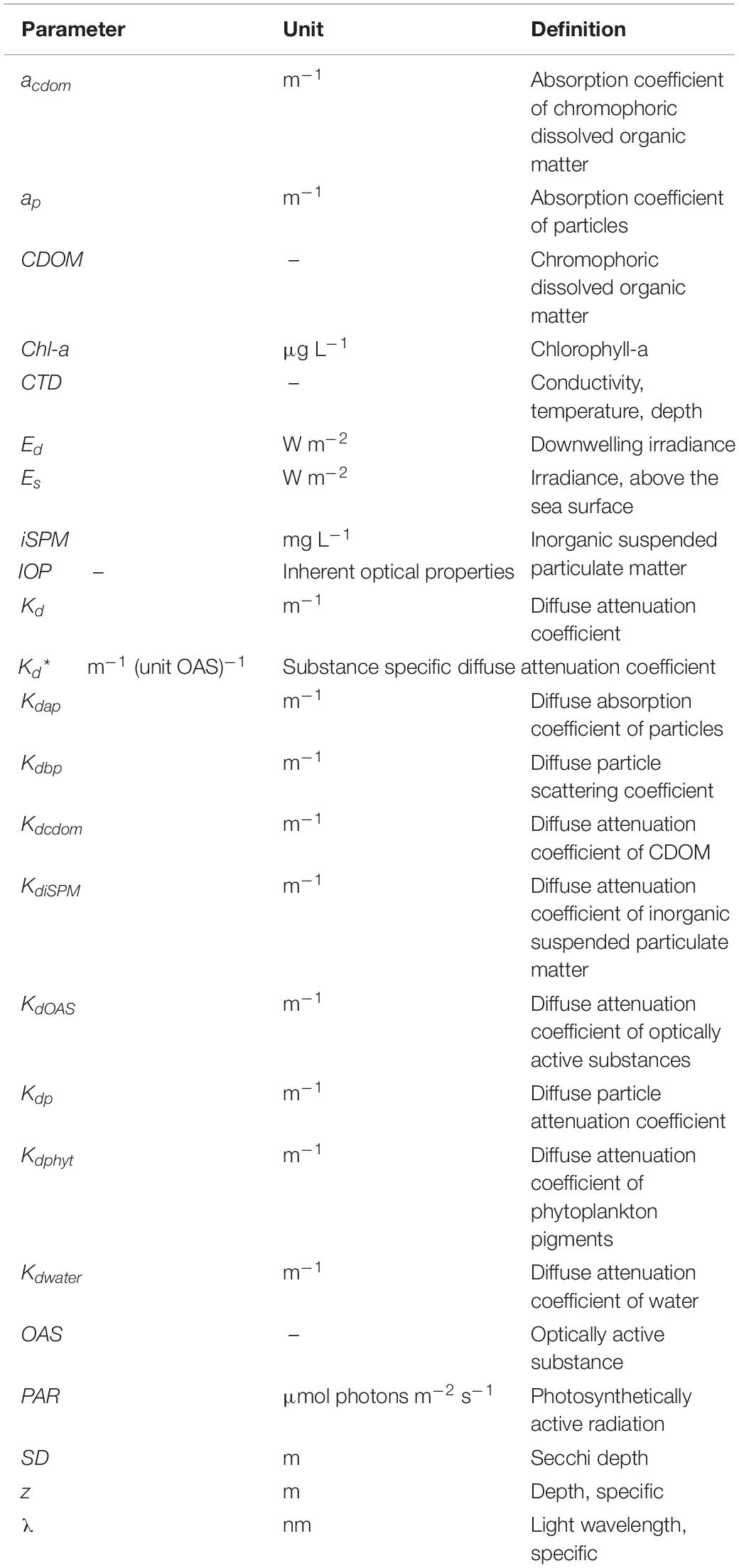
Table 1. List of regularly used abbreviations.

When light enters the water column, it is subject to scattering and absorption (summarized as attenuation), which lead to a reduction of PAR with depth. This reduction can be described by an exponential function (e.g., Kirk, 2011):

$$PAR\left(z\right)=PAR{\left(0^{-}\right)}^{*}\exp -K_d{\left(PAR\right)}^{*}z{\left(0\right)}^{*}\exp -K_{dPAR}^{*}z$$

Here, z is the depth in which the light availability is going to be calculated, PAR(0^–) is the light just below the surface, and K_d (PAR) is the diffuse attenuation coefficient of PAR (in m^–1). K_d (PAR) depends on the degree by which the downwelling light is absorbed and scattered by the water itself, but also by the optically active substances (OAS) that are present therein (Mobley, 1994; Kirk, 2011; Zielinski, 2013). In the photosynthetic relevant part of the light spectrum, these constituents are mainly phytoplankton with its various pigments, especially chlorophyll-a (chl-a), but also chromophoric dissolved organic matter (CDOM), as well as non-algal particles like detritus and inorganic suspended particulate matter (iSPM). K_d (PAR) can be thought of being composed of the diffuse attenuation coefficients of water and these OAS. However, the attenuating properties of these substances are not equal over the range of PAR: Pure water attenuates predominantly at wavelengths >600 nm, while the absorption of all OAS generally increases toward the shorter wavelengths (but in various intensity). Scattering of CDOM is negligible compared to its absorption, although due to the small size of the molecules (per definition <0.2 μm), the scattering efficiency of the shorter wavelengths is higher. The scattering properties of larger particles like phytoplankton cells and iSPM are less wavelength depended, but their contribution to light attenuation can be high, especially in coastal areas (Kirk, 2011). Thus, an accurate representation of light attenuation with depth requires the use of a spectrally resolved attenuation coefficient [K_d (λ)], which can be obtained by taking hyperspectral measurements of the downwelling irradiance [E_d (λ)] in various depths (Lee et al., 2005; Kirk, 2011). Spectral light availability in dependence of waters OAS can be modeled by using radiative transfer equations, as implemented in software like HydroLight-EcoLight (Mobley, 1994).

Nevertheless, for many applications like calculating photosynthetic rates or primary productivity, only the bulk parameter PAR is used. Although it has been shown that the use of spectral light data significantly alters the result of ecosystem models (Mobley et al., 2015), there are a couple of reasons for using spectrally integrated, thus PAR-based approaches. This includes on the one hand the sparsity of available spectral data and the greater effort in evaluating a spectral model (Thewes et al., 2020), but also the increase in computational effort. Although the latter point will probably become less important with technological progress, to date it is still a limiting factor, both with respect to time and costs.

A common way of expressing vertical light attenuation in biogeochemical models is to parameterize K_d (PAR) with OAS that are part of the model (e.g., Fasham et al., 1990; Kühn and Radach, 1997; Zielinski et al., 2002). However, in many cases, only chl-a as representative of phytoplankton biomass is considered, what potentially limits the use of these parameterizations in coastal waters, where constituents like CDOM and iSPM contribute largely to light attenuation and also do not necessarily co-vary with phytoplankton abundance (case II waters; Morel and Prieur, 1977; Mobley, 1994). Furthermore, unweighted attenuation of PAR completely ignores the spectral dependence of the attenuation properties of the different OAS. In attempting to overcome this issue while still considering computational efficiency, bi- and multimodal parameterizations have been developed (Paulson and Simpson, 1977; Morel, 1988; Zielinski et al., 2002; Dutkiewicz et al., 2015), which have shown to be advantageous. In such approaches, the PAR spectrum is divided into two or more spectral bands, either equally spaced or driven by considerations related to the attenuation properties of the OAS. Then, for each band, a separate K_d is parameterized using the OAS of relevance. When subsequently modeling the attenuation of PAR with depth, its scalar surface value is proportionally divided according to the size of the spectral bands, and the K_d values are applied separately.

In this study, the results of underwater light field and water constituent measurements made along onshore-offshore transects in a coastal environment (North Sea) are shown. The collected data were used to parameterize the attenuation of PAR in a novel trimodal approach in order to obtain a sufficiently accurate, but still computational affordable representation of light attenuation in coastal waters for modeling purposes. The trimodal parameterization includes chl-a, iSPM, and also salinity as proxy for CDOM (Bowers et al., 2004), taking into account the typical V-shape of spectral K_d (λ) in coastal areas. In the mid-part of the spectrum usually the minimum of K_d (λ) is observed, which determines the visible transparency of the water as determined by Secchi disk measurement (Lee et al., 2015). This potential connection between modern model calculations and historical Secchi disk data was a further rationale for choosing the trimodal approach. Modeled PAR profiles using the trimodal approach are compared to measured data, but also to the profiles modeled with a monomodal and a spectral parameterization approach. Finally, strengths and weaknesses of the chosen approach are discussed.

Materials and Methods

Research Area

The research area covers the southern and central North Sea as well as parts of the British and Irish coasts. Data were collected on discrete stations during three cruises with the research vessel “Heincke” (Knust et al., 2017; HE503: February/March 2018, HE516: July/August 2018, and HE527: March 2019; hereafter denoted as Winter, Summer, and Spring cruise). Thus, a wide range of different conditions is represented in the dataset used for this study. Figure 1 shows the position of the stations which were considered for data analysis. Taking into account the different sampling depths, the total number of observations were n = 31/219/75 (Winter/Summer/Spring). However, not all parameters were available at each station, therefore the actual number of observations varies between the analyses.

FIGURE 1

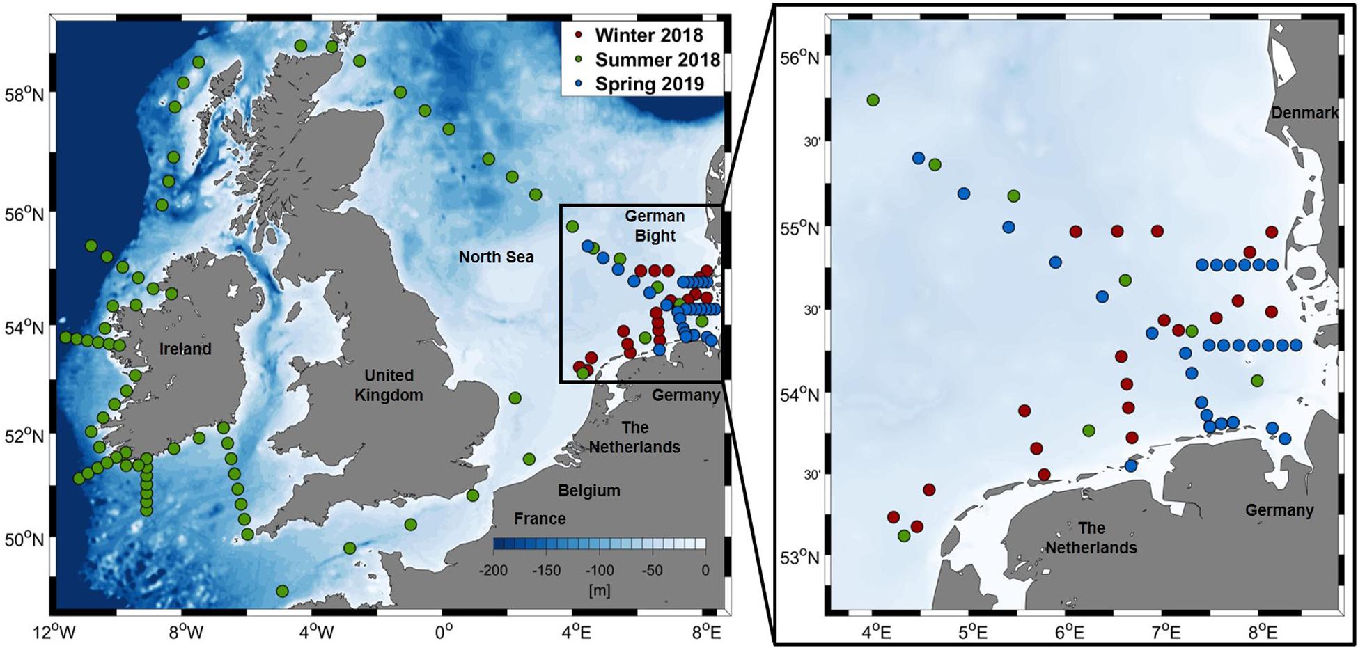
Figure 1. Area of research with sampling stations, categorized by cruise (left), close-up of the German Bight area (right).

Measurements of Underwater Light Field

Hyperspectral profiles of the underwater light field were taken in the range of 346–800 nm using a free falling profiling instrument (HyperPro II, Seabird Scientific, United States). It is equipped with a planar (cosine) radiometer for measuring downwelling irradiance E_d (λ) and a radiance-type radiometer with a field-of-view of 8.5° for measuring upwelling radiance L_u (λ). Furthermore, a reference irradiance sensor (identical to the E_d sensor) was attached to the upper deck of the ship to measure the available light above the sea surface E_s (λ). For this study, only data covering the range of PAR (400–700 nm) were considered. The HyperPro II has further mounted sensors for measuring conductivity, temperature, and pressure, as well as an ECO Puck (Seabird Scientific, United States) with channels for chlorophyll fluorescence (excitation 470 nm and emission 695 nm), CDOM fluorescence (excitation 370 nm and emission 460 nm), and backscattering (at 700 nm). The deployment of the profiler followed the protocols given in Holinde and Zielinski (2016) and Mascarenhas et al. (2017): Per station, at least three profiles were taken. Before starting the measurements, the ship was positioned with the stern to the sun to avoid ship shadow on the profile area and the reference sensor. The profiler’s pressure sensor was tared on deck with the instrument being in an upright position. The profiler was deployed by its own drift in approximately 30 m distance to the ship, before it was lowered in free-falling mode with a speed of approx. 0.5 m/s. Profiles were taken as deep as possible, but at least to the depth which is reached by 1% of surface (above water) PAR. Data obtained during an instrument tilt >10° was omitted from the dataset.

In order to account for changes in ambient light during the profile, E_d (λ) was normalized to E_s (λ) measured by the reference sensor (Mueller et al., 2003). Quality control was performed per wavelength according to the procedure suggested by Organelli et al. (2016) for radiometric data obtained from ARGO-floats. Profiles were extrapolated to the surface using the logarithm of the data points with the highest quality (flag 1) and a 2nd order polynomial fit. E_d (λ) data was smoothed spectrally using a moving median (window size: 7 nm) and subsequently, PAR was calculated by converting energy spectra of E_d (λ) (W/m² s) in photon flux density spectra (μmol photons/m² s) and integrate the spectrum from 400 to 700 nm. Profiles of K_d (λ) and K_d (PAR) were calculated as local slopes from the E_d (λ) and PAR profiles, respectively (Smith and Baker, 1984, 1986), using a half interval of 1 m. E_d (λ) and K_d (λ) from the obtained profiles were inspected manually for the respective sampling depths (see below), the most reasonable spectrum was used in the parameterization.

Additionally, Secchi depth (SD) was measured as indicator for water transparency. For this, a white disk of 30 cm diameter was lowered into the water up to the point where it was no longer visible. This depth was noted as SD.

Determination of Optically Active Substances and Absorption Coefficient Spectra

In order to link the light field measurements with the IOPs and OAS, water samples were taken at the stations using a carousel water sampler equipped with a CTD system (SBE911plus, Seabird Scientific, United States) including sensors for conductivity, temperature, pressure, oxygen, chl-a fluorescence (ECO-FL, excitation 470 nm, emission 695 nm, Seabird Scientific, United States), and beam transmission (C-Star, 650 nm, Seabird Scientific, United States). Up to three depths were sampled: The first sampling depth was 4–5 m, the second the depth in which a potential chlorophyll maximum occurred, and the third was the bottom depth. Not all depths were sampled on each station (e.g., in case the water column was thoroughly mixed); the decision was made based on the online data of the CTD sensors.

The sampled water was processed directly on board. For chlorophyll-a determination, aliquots of 0.2–10 L (depending on concentration of particulate matter) were filtered on pre-wetted glass fiber filters (47 mm diameter, pore size approximately 0.7 μm; Whatman, United Kingdom) and were subsequently frozen and stored at −80°C. Pigment extraction was done within 6 months after the cruise in 90% acetone-water solution with overnight incubation at 4°C. Additionally, extracts from empty filters were prepared as blanks. Extracts were centrifuged for 10 min at 3,020 × g and the fluorescence of the supernatant was determined at 665 nm before and after acidification of the samples using a pre-calibrated TD-700 laboratory fluorometer (Turner Designs, San Jose, CA, United States). On the basis of these measurements, chl-a concentration was calculated according to Arar and Collins (1997), taking into account the results from the blank filters. For SPM determination, pre-washed, pre-combusted, and pre-weighted filters of the same type as for chl-a analysis were used. After wetting the filter with purified water to prevent the accumulation of salt on the rim as much as possible, aliquots of 0.2–17 L sample water were filtered. After filtration, the filter was rinsed with purified water (>50 mL) to avoid salt remains. Subsequently, the filters were frozen and stored at −25°C, and SPM concentration was determined gravimetrically in the laboratory directly after the cruise. In order to obtain the concentration of iSPM afterward, the organic fraction was removed by combusting the filters at 450°C for 8 h, and the gravimetric analysis was repeated.

Water samples were further analyzed onboard with a custom-built PSICAM (Kirk, 1997; Röttgers et al., 2005) in order to obtain the total, particulate, and CDOM absorption coefficients hyperspectrally and free of scattering errors in a range of 400–700 nm. The specifications of the PSICAM used are described in Wollschläger et al. (2019). The measurement procedure was identically with that described in Röttgers and Doerffer (2007), while the calibration was made using a solid standard instead of the nigrosin solution (Wollschläger et al., 2019). Total spectral absorption coefficients a (λ) were determined by measuring an unfiltered water sample (approximately 450 mL), while CDOM spectral absorption coefficients [a_cdom (λ)] was determined after filtration of the sample through a 0.2 μm membrane filter (Whatman, United States. The difference between the two measurements is considered the particulate absorption a_p (λ). The CDOM absorption at 440 nm [a_cdom (440)] was initially used as a proxy for CDOM concentration, however, for the parameterization the complete spectrum was used.

Per station, depth profiles of chl-a and iSPM were generated by correlating the laboratory data with the corresponding in situ chl-a fluorescence and beam transmission data. In order to have a positive correlation between beam transmission and iSPM concentration, the beam transmission was inverted to attenuance (1-transmission) and expressed in percent. CDOM profiles were created by correlations between different parts of a_cdom (λ) and practical salinity (calculated from CTD temperature and conductivity), as in coastal areas, the main sources of CDOM are riverine input and terrestrial runoff. All in situ data have been smoothed moderately in advance to remove spikes using a cubic smoothing spline, following the recommendations given in the MATLAB documentation for the “csaps.m” function, which was used for this purpose. Afterward, the profiles have been checked for reasonability by manual inspection.

Decomposition of K_d Spectra

In this study, it is assumed that K_d (λ) is linearly composed of the absorption and scattering contributions of phytoplankton (represented by chl-a concentration), CDOM (represented by salinity), iSPM, and water.

$$\begin{array}{c}{K}_d(\text{λ})=K_{dwater}(\text{λ})+K_{dcdom}(\text{λ})\\ +K_{dphyt}(\text{λ})+K_{diSPM}(\text{λ})\end{array}$$

We are aware that this is only a simplification as shown recently by Lee et al. (2018), however, this approach was chosen in order to keep the model as simple as possible. For the parameterization of K_d (λ) using the mentioned variables, it is necessary to establish substance-specific diffuse attenuation coefficient values (K_d^∗) for the selected spectral regions. For this, K_d (λ) measured at the stations have to be decomposed with respect to the contributions of the single OAS. The procedure relies on measurements of the absorption coefficients, as K_d (λ) is a function of the inherent optical properties absorption (a) and backscatter (b_b), with a > > b_b (Mobley, 1994). It is described in the following, a visual summary is given in Figure 2.

FIGURE 2

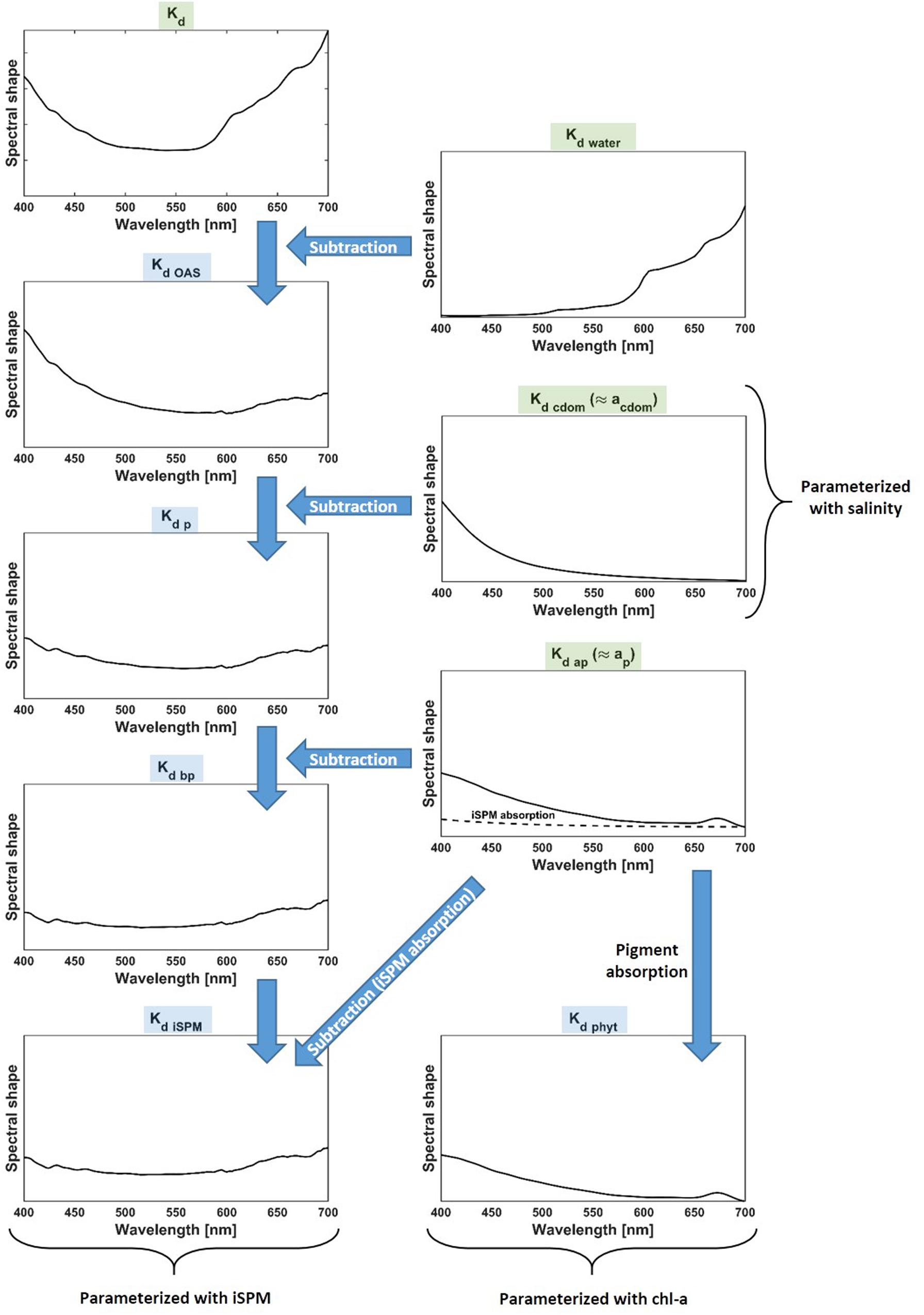
Figure 2. Decomposition of K_d (λ) in spectra associated to the various optically active constituents [K_{d water} (λ), K_{d cdom} (λ), K_{d phyt} (λ), and K_{d iSPM} (λ)]. The arrows indicate which parameter has been taken into account for deriving the respective decomposition step. Parameters highlighted in green originate from measurements, while the parameters highlighted in blue are derived from the decomposition.

As the water attenuation spectrum is known from literature (Morel and Maritorena, 2001), it can be subtracted from K_d (λ) to obtain the attenuation coefficient spectrum of the OAS [K_{d OAS} (λ) = K_d (λ) − K_{d water} (λ)]. K_{d OAS} (λ) has to be subsequently divided in K_{d cdom} (λ), K_{d phyt} (λ), and K_{d iSPM} (λ). Because CDOM is nearly dissolved in water, its attenuation can be thought of being largely driven by its absorption properties. Thus, a_cdom (λ) determined by PSICAM measurements can be assumed to be identical with K_{d cdom} (λ). Its subtraction from K_{d OAS} (λ) gives the diffuse particle attenuation coefficient K_{d p} (λ) composed of the absorption and scattering properties of phytoplankton cells and iSPM [K_{d p} (λ) = K_{d OAS} (λ) − K_{d cdom} (λ)]. The contribution of detritus is neglected at this point, as it is small compared to that of the other components. The particle absorption coefficients a_p (λ) have been directly measured with the PSICAM, and under the assumption that they are identical with the diffuse particle absorption coefficients K_{d ap} (λ), they are subtracted from K_{d p} (λ) to obtain K_{d bp} (λ), the diffuse particle scattering coefficient [K_{d bp} (λ) = K_{d p} (λ) − K_{d ap} (λ)]. Theoretically, K_{d bp} (λ) summarizes the scattering of phytoplankton and iSPM, but the scattering in coastal waters is usually much stronger determined by iSPM due to its higher refractive index (Kirk, 2011). For this reason, and as we have no means to decompose K_{d bp} (λ) further, it is regarded to be completely related to iSPM for our purposes. Similar to the diffuse particle scattering coefficient, the diffuse absorption coefficient K_{d ap} (λ) is also composed of the contributions of phytoplankton and iSPM. The latter can become significant, especially in coastal areas with high sediment loads. For the decomposition of K_{d ap} (λ) in the iSPM and phytoplankton part, respectively, the phytoplankton absorption is assumed to be largely driven by the phytoplankton pigments, neglecting contributions of non-pigmented phytoplankton parts (e.g., cell walls). Since phytoplankton pigment absorption is close to zero at wavelengths >700 nm (Babin and Stramski, 2002; Röttgers et al., 2007; Clementson and Wojtasiewicz, 2019), any absorption that is still visible at this wavelength can be thought to be related to iSPM. Because the absorption of inorganic matter increased exponentially toward the shorter wavelengths, a full iSPM absorption spectrum can be extrapolated based on a_p(700) as well as the equation and the mean slope provided by Bowers and Binding (2006). The constructed iSPM absorption coefficient spectrum is then added to the scattering part of K_{d bp} (λ) to obtain K_{d iSPM} (λ) [K_{d iSPM} (λ) = K_{d bp} (λ) + K_{d ap (iSPM)} (λ)]. What remains is the diffuse attenuation coefficient of the phytoplankton pigments K_{d phyt} (λ).

The derived spectra of K_{d cdom} (λ), K_{d iSPM} (λ), and K_{d phyt} (λ) are subsequently related to the respective OAS (in case of CDOM with the proxy parameter salinity) by linear regression, in order to obtain the K_d^∗ values required for the model formulation (see section “Deriving Substance-Specific K_d Values for the Different Optically Active Substances”).

Results and Discussion

Diffuse Attenuation Coefficient Spectra

K_d (λ) has been calculated from E_d (λ) profiles obtained during the three cruises. The values ranged from 0.04 to 1.95 m^–1, with considerable spectral variability (Figure 3, left panel). Generally, the values increased toward the blue and the red part of the spectrum, with minima in the range of 480 to 580 nm (Figure 3, right panel). The increase toward the shorter wavelengths was smaller for most of the stations from the summer cruise. Despite the quality control and smoothing of E_d (λ) before K_d (λ) calculation, some of the spectra still show artifacts or noise, especially in the red above 650 nm, and to a lesser degree also in the blue below 450 nm. Furthermore, not all spectra extend over the full range of PAR, as extremely noisy data did not pass the quality control. In the red spectral region light is already rapidly attenuated in the first few meters by the water itself. Therefore it is generally difficult to obtain reliable light field measurements in this region (Mueller et al., 2003), an effect that is increased by the presence of other light absorbing compounds. Similarly, as in coastal areas the concentration of OAS is commonly high compared to the open ocean, this effect can also be seen in the blue region, where the OAS dominate attenuation. However, as for the parameterization the median of a certain spectral range is used, the impact of artifacts or even incomplete spectra on the final result becomes smaller.

FIGURE 3

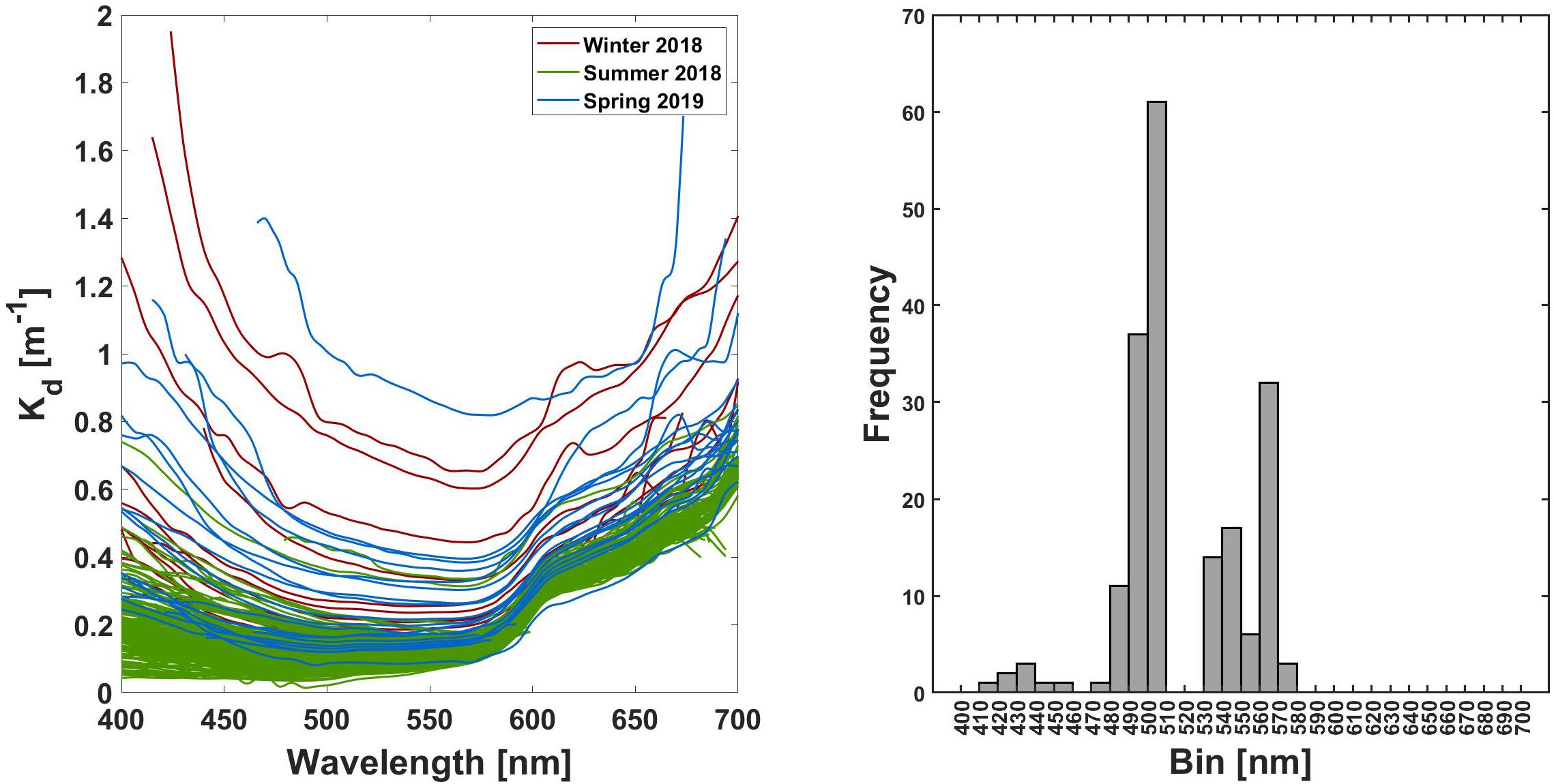
Figure 3. Overview of K_d (λ). Spectra obtained at the sampling sites (left). Histogram of K_d (λ) minimum wavelength distribution (right).

Relationships Between Optically Active Substances and in situ Proxies

Directly, the OAS were determined only at stations in various depths by discrete sampling. However, for modeling PAR profiles based on these substances and the established substance-specific attenuation coefficients (see section “Assessment of the Model Approaches”), depth-resolved OAS data is necessary. For this reason, the discrete measurements were correlated with the values of the in situ proxies in the respective depth (chl-a fluorescence for chl-a, beam attenuance for iSPM, and salinity for CDOM). The obtained coefficients allow a conversion of the proxy data profiles into OAS profiles. For chl-a and CDOM, linear regressions were used, while for iSPM, a more accurate representation was a polynomial fit of second order. Data were analyzed together but also separated by cruise (Figure 4). Potential outliers have been identified by analyzing the residuals of the linear regressions from the individual cruises. If the residual of a certain data point was outside of the residual mean ± 2 times their standard deviation, the data point was considered as being an outlier. For the sake of showing the complete dataset, they are displayed in Figure 4 as crosses, but were not taken into account for the final regressions.

FIGURE 4

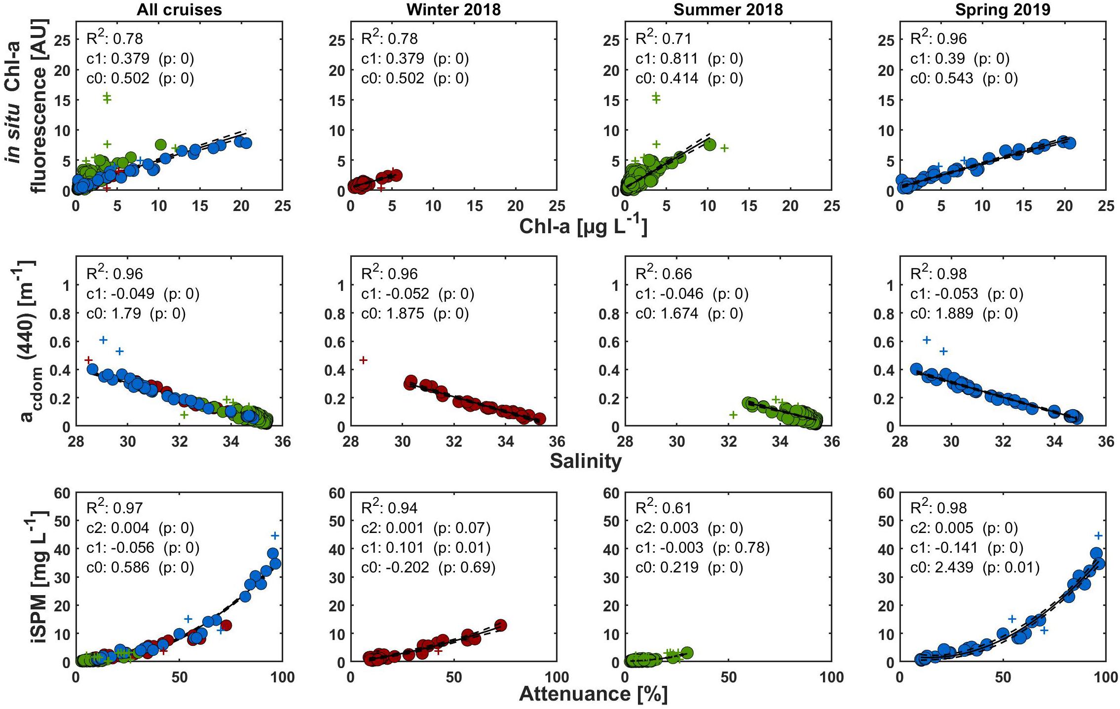
Figure 4. Correlations between optically active substances and their respective in situ proxies. Data points considered as outliers (see text) are displayed as crosses and are not included in the fit represented by the solid line. The dashed lines give its 95% confidence interval. AU means that chl-a fluorescence is given in arbitrary units.

Chl-a concentrations were found to be 0.16 to 20.6 μg/L over all cruises, with considerably narrower ranges in Winter and Summer 2018 (Figure 4, upper panels). There were reasonable linear correlations with in situ chl-a fluorescence for all three cruises as well as for the combined dataset, with R² values ranging from 0.71 to 0.96. The offset (c0) in the data was similar, what was to be expected as the instrument used was identical and checked, but not recalibrated between the cruises. Interestingly, the slope (c1) was considerably higher in Summer 2018 than in the two other cruises, and also in the combined dataset. This indicates a real change in the ratio of chl-a to in situ chl-a fluorescence, which can occur due to differences in community composition, light acclimatization, and nutritional status of the phytoplankton (Kiefer, 1973; Soohoo et al., 1986; Cunningham, 1996). All these factors can vary with both season and location, and in fact, both the time and the study area of the Summer cruise were considerably different from the others. In contrast, the timing of the Winter and Spring cruise was similar, and so was the slope of the linear regression.

Regarding CDOM, here given as a_cdom (440) ranging from 0.01 to 0.61 m^–1, the results for the linear regressions were quite similar in all three cruises: CDOM was inversely related to salinity with a slope ranging between −0.046 and −0.053, while the offset was between 1.674 and 1.889 with R² between 0.66 and 0.98. This inverse relationship is to be expected under conservative mixing conditions when the dominant source of CDOM is riverine input and runoff from land (Liss, 1976; Stedmon and Markager, 2003; Bowers et al., 2004). In this form, it is a typical feature of European coastal waters and would have to be validated for other coastal regions. Furthermore, the slope of this relation can vary according to the optical properties of the CDOM, which are in turn influenced by, e.g., its chemical composition and degradation processes (Helms et al., 2008 and references therein). Thus, it is to a certain extent region-specific. In more offshore regions, other processes than conservative mixing (e.g., autochthonous production by phytoplankton) start to determine CDOM distribution, what weakens the relationship between salinity and CDOM. In this context, the strikingly higher variability and the less negative slope of the Summer cruise (Figure 4) compared to the others might be explainable with a higher number of offshore stations, and a general shift in research area (compare Figure 1). However, as the correlation applied to the pooled data indicates, salinity is still a sufficient proxy for CDOM absorption the investigated area. Of course, the relationship shown in Figure 3 is only an example, because as CDOM absorption is a spectral parameter, its relationship to salinity varies with wavelength. Fits between salinity and other a_cdom (λ) wavelengths were of similar quality with R² values in the range of 0.75 to 0.96, but with different slopes and offsets (data not shown). Therefore, it is not accurate to use only a selected wavelength to convert salinity into CDOM, as its influence on light attenuation varies over the spectrum. Therefore, salinity was directly parameterized as a representative of CDOM in the different approaches (see section “Deriving Substance-Specific K_d Values for the Different Optically Active Substances”).

Concentrations of iSPM varied between 0.02 and 40.52 mg L^–1. Highest concentration was obtained in the southern German Bight near the barrier islands and the Elbe estuary, while they were lowest off the continental shelf west of Ireland. Like the correlation of CDOM and salinity, the correlation for iSPM and beam attenuance was more variable in the Summer cruise than in the Winter and Spring cruise (R² of 0.59 compared to 0.94 and 0.98, respectively). This might also be caused by a more variable particle composition due to the more heterogeneous study area, but maybe also because of a smaller data range covered.

As a consequence of the variability between the cruises, the conversion of in situ data into OAS was done with the cruise specific coefficients, not with the coefficients obtained for the pooled dataset.

Deriving Substance-Specific K_d Values for the Different Optically Active Substances

In order to parameterize K_d (λ) on the basis of OAS concentration, it was decomposed in K_{d water} (λ), K_{d cdom} (λ), K_{d phyt} (λ), and K_{d iSPM} (λ) as described above (see section “Decomposition of K_d Spectra”). Subsequently, the median was taken (i) from the complete spectra (monomodal approach), (ii) from three spectral bands (trimodal approach), or (iii) the data were used in 1 nm resolution (spectral approach). The median was used instead of the mean, since it leads to a parameterization that provided model results more closely to the measured data, as has been found in the later assessment (not shown). The substance-specific K_d values (K_d^∗) for all approaches were derived by applying linear fits to correlations of the median or spectral K_d data with chl-a concentration, salinity (directly parameterized as a proxy of CDOM), and iSPM concentration, respectively.

As the trimodal approach is the focus of this study, the results of these fits (Figure 5, Table 2) will be discussed in more detail. Nevertheless, the coefficients of the monomodal approach are given in Table 3, while that of the spectral approach are given in the Supplementary Material. With exception of K_{d cdom}, all fits were performed without intercept, assuming no contribution to K_d when the respective OAS is not present. This is justified, because calculations including an intercept showed that it was low in all cases and not statistically significant (p > 0.05, data not shown). K_d^∗ of the OAS was considered to be the slope of the respective fit (p < 0.05 in all cases).

FIGURE 5

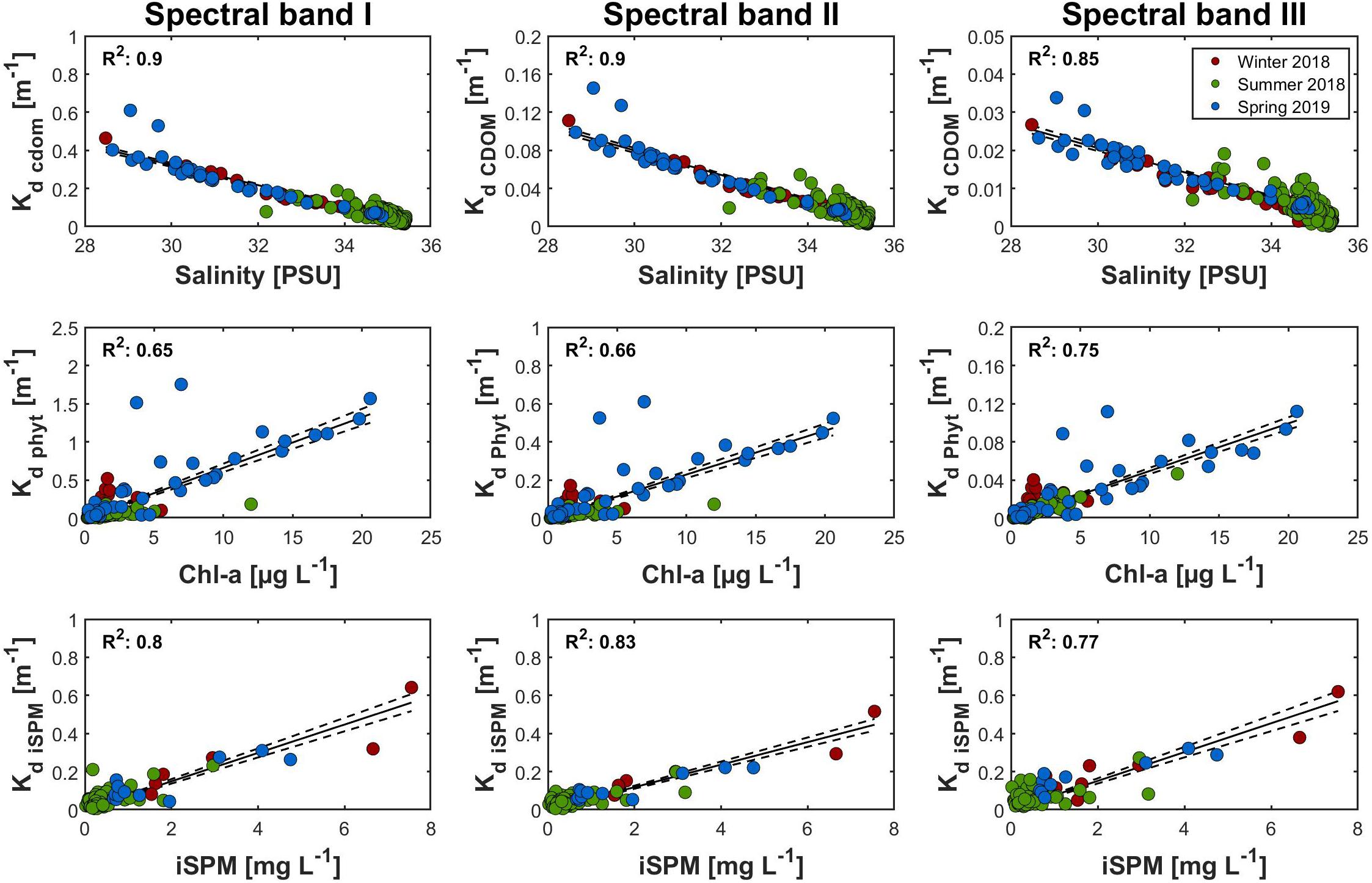
Figure 5. Linear fits between the optically active constituents (CDOM represented by salinity) and their median K_d values in the three spectral bands. The solid line represents the linear fit, while the dashed lines give its 95% confidence interval.

TABLE 2

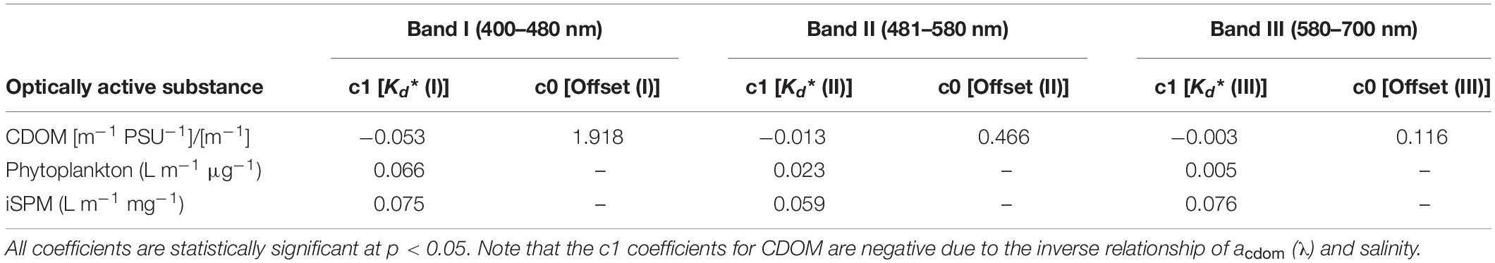
Table 2. Summary of the substance-specific diffuse attenuation coefficients (K_d*) for different OAS in the trimodal approach.

TABLE 3

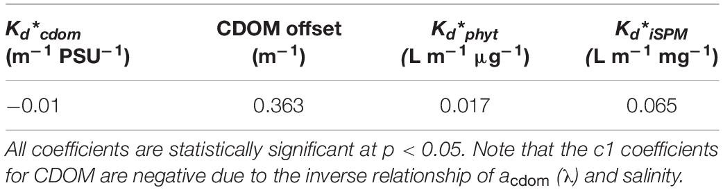
Table 3. Summary of the substance-specific diffuse attenuation coefficients (K_d*) for different OAS in the monomodal approach.

The range of the bands in the trimodal approach was not determined arbitrary, but was based on the spectral shape of K_d (λ). As shown in Figure 3, the majority of the spectra had their minimum value between 481 and 580 nm, which justifies this wavelength range to be defined as a spectral band (K_d II). On that basis, K_d I is the band covering the shorter wavelengths (400–480 nm), while K_d III covers the longer wavelengths (581–700 nm). Although the bands have been derived from this specific dataset, they are probably suitable also for other coastal environments. Due to sampling in different seasons and at different locations, a certain variability in K_d (λ) is already included in the data and thus considered in the definition of spectral band II (and thus the other two bands). Even if the optical properties defining the spectral shape of K_d (λ) might change to a certain extent with region, the general characteristic of having a minimum in the greenish wavelengths should persist.

It can be seen that K_d^∗(I) > K_d^∗(II) > K_d^∗(III) for all OAS with the exception of iSPM, where K_d^∗ in spectral band III is as high as in band I. Normally, it would be expected of K_{d iSPM} (λ) to decrease slowly with increasing wavelength, because this is the shape of the iSPM absorption coefficient spectrum, while the scatter spectrum is uniform over the wavelengths or has (due to Rayleigh scattering) also an decrease toward the longer wavelengths. However, as it is exemplarily shown in Figure 2, the K_{d iSPM} (λ) spectrum that results from the decomposition of total K_d (λ) increases again toward the longer wavelengths, what is consistent with the observed higher K_d^∗_iSPM in band III compared band II. This results probably from the fact that the simple addition (or in this case: subtraction) of the K_d (λ) contributions of the OAS are only an approximation, which is not fully consistent with radiative transfer theory (Lee et al., 2018). As demonstrated in the named publication, there are especially differences toward the red part of the spectrum, what fits to the observations made. Another source of discrepancy could be that K_d (λ) measurements and water sampling for the absorption coefficient measurements have not been performed at exactly the same location or time. The profiler was deployed approximately 30 m away from the ship, and the light profiles were taken approximately 45 min after the start of the CTD. However, this might have contributed to general variability in the data, but not to deviations specifically in the red part of the spectrum. But in general, a major part of all uncertainties associated with the measurements and the decomposition procedure are summarized in the K_{d iSPM} (λ) parameter, as it is the last one that is derived in the course of the decomposition. Nevertheless, as light in spectral region III is anyway attenuated rapidly with depth due to the water itself (K_{d water} (III): 0.31 m^–1) and, in coastal areas, due to high iSPM concentration, the slight overestimation of K_d^∗_iSPM (III) can be considered of minor importance.

The relationship of salinity and K_{d cdom} (I/II/III) becomes more variable in the high-saline regions (Figure 5, upper panels). Especially data points belonging to the Summer 2018 cruise are often located above the linear fit established for the whole dataset. This might indicate an increasing contribution of autochthonous production of CDOM by phytoplankton that weakens the conservative relationship between CDOM and salinity valid in the more coastal (less saline) waters. This has implications for the performance of the trimodal model approach with the proposed coefficients in these areas. However, the effect should be comparably small, as in spectral band I, where the impact of CDOM (and thus K_d^∗_cdom) is the highest, the variability in the high saline waters is still comparably small. Although the variability becomes higher in spectral bands II and III, its effect on the performance of the parameterization should be still low, as the coefficients itself are much smaller than in band I.

Compared to the other OAS, the relationship between chl-a and K_{d phyt} (I/II/III) is the most variable. As K_d^∗_phyt is basically identical with the chlorophyll-specific absorption coefficient (see the description of the decomposition procedure), also its sources of variability are the same. First of all, K_{d phyt} (λ) is not only determined by chl-a, but is influenced by the occurrence of other photosynthetic and photoprotective pigments, as well as with the pigment packaging effect (Morel and Bricaud, 1981; Bricaud et al., 1995, 2004; Kirk, 2011). Thus, factors like phytoplankton taxonomical composition (spatial differences and seasonal succession) and light acclimatization contribute to the variability of K_d^∗_phyt (I/II/III). For this reason, the highest uncertainty in the parameterization is probably associated with the values of K_d^∗_phyt (I/II/III). In general, although the coefficients in this study have been derived from a dataset that already contains a certain regional and seasonal variability, the inclusion of additional data from other coastal areas would be beneficial to assess their general validity.

Assessment of the Model Approaches

In order to evaluate the performance of the monomodal, trimodal, and spectral approach to describe the attenuation of PAR with depth, a comparison between modeled and measured PAR profiles was made. For the trimodal approach, the modeled PAR profiles were calculated for each station from surface to the maximum depth of the measurements according to:

$$\begin{array}{c}PAR(z)=PAR(0^{-})*[0.27\exp (-K_d(I)*z)+0.36\exp \\ (-K_d(II)*z)+0.37\exp (-K(III)*z)]\end{array}$$

The factors 0.27, 0.36, and 0.37 represent the proportions of the three spectral bands to total PAR. They were derived by normalizing E_d (λ, 0^–) of all stations to the mean of E_d (λ, 0^–) over the whole dataset. Subsequently, these normalized spectra were integrated over the complete spectral range (giving PAR) as well as over the wavelengths constituting the spectral bands (giving the fraction of PAR that corresponds to the size of the respective band). The proportion of each integrated band to the total integrated spectrum was calculated for each station, and the median values were included in the equation above. In order to calculate PAR in a given depth, PAR(0^–) was partitioned proportionally to the size of the bands using these factors, and the bands were attenuated independently of each other down to that depth, before the values are finally summarized into PAR. The K_d profiles of the bands were calculated using the respective substance-specific coefficients (Table 2) and the in situ data acquired with the CTD. Chl-a fluorescence and beam attenuance have been converted in chl-a and iSPM concentration profiles for that purpose (see section “Relationships Between Optically Active Substances and in situ Proxies”).

$$\begin{array}{c}{K}_d=\left(K_d^{*}{}_{water}z\right)+\left(K_d^{*}{}_{cdom}{\displaystyle {\int }_0^{z}Salinity(z\text{'})}+SalinityOffset\right)\\ +\left(K_d^{*}{}_{phyt}{\displaystyle {\int }_0^{z}Chl-a(z\text{'})dz\text{'}}\right)+\left(K_d^0{}_{iSPM}{\displaystyle {\int }_0^{z}iSPM(z\text{'})dz\text{'}}\right)\end{array}$$

For clarity, the designation of the bands (I/II/III) have been omitted in the equation above.

The modeling of PAR profiles with the monomodal and spectral approach have been performed in a similar manner. However, for the monomodal approach no partitioning of PAR(0^–) was performed and only one K_d profile valid for the whole spectrum was calculated using OAS concentrations and OAS-specific K_d^∗ (Table 3). For the spectral approach, PAR(0^–) was partitioned in 301 bands (corresponding to a resolution of 1 nm) using a factor of 0.0033, and K_d profiles were calculated individually for each wavelength (for wavelength-specific K_d^∗ values see Supplementary Material).

Examples of typical measured and modeled PAR profiles are illustrated in Figure 6, showing overestimation, match, and underestimation of PAR by the model. In order to quantify these differences, both profiles were integrated over the investigated water column at all stations, basically obtaining two scalar values representing the measured and estimated amount of light present per station. The difference between model results and measurements were then expressed as percentage of the measurements. Thus, for example, a perfect match at a given station would result in a value of 0%, while ±10% means a 10% over- or underestimation of integrated PAR over the water column by the model data.

FIGURE 6

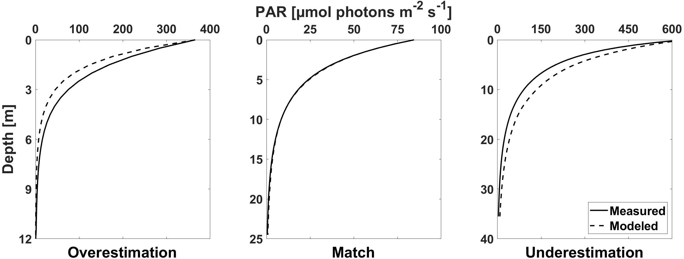
Figure 6. Examples of measured and modeled PAR profiles at selected stations. Overestimation of available PAR by the trimodal approach (left), match of model and measurements (center), and underestimation (right).

When comparing the three approaches in this respect, it can be seen that the trimodal approach performs similar to the spectral approach, while the monomodal approach overestimated the available light much more. The median differences to the measurements were 50, 8, and 6% for the monomodal, trimodal, and spectral approach, respectively (Figure 7). In addition, also the spread in the differences was considerably higher in the monomodal (−30 to 110%) than in the other approaches (approximately −40 to 50%). Thus, while K_d (PAR) is on average estimated correctly by the spectral and trimodal approach, it is systematically underestimated by the monomodal approach. Obviously, taking the median of K_d (λ) from the different OAS during the parameterization lead to K_d^∗ values that were too low to model light attenuation with depth correctly. The spread of the data in the boxplots (thus the variability in the differences) is related on the one hand to the variability of the OAS specific attenuation coefficients (Figure 5 for the trimodal approach). They describe only an average attenuation of a specific concentration of a substance (represented by the slope of the fit). However, at a specific site, the properties of the OAS might deviate from this average. On the other hand, it has to be taken into consideration that not only the quality of the K_d^∗ values and thus the parameterization is responsible for any differences observed between measured and modeled PAR, but also the quality of the available OAS data. For an ideal evaluation of the model performance, direct measurements of OAS (pigment concentration and gravimetry of suspended matter) in high vertical resolution would be desirable. In practice, this would require an unrealistic high effort for a suitable number of profiles. Thus, the common way is to measure (optical) proxies which are then converted into OAS concentrations, as done in this study. However, this transfers any variability between the optical proxy and its OAS in the evaluation of the model performance, e.g., changes in the relation between chl-a fluorescence to chl-a due to vertical changes in phytoplankton composition or due to non-photochemical quenching. Thus, the assessment made here primarily compares the approaches with each other, and the performance of the modeling approaches might be even better than implied by our evaluations.

FIGURE 7

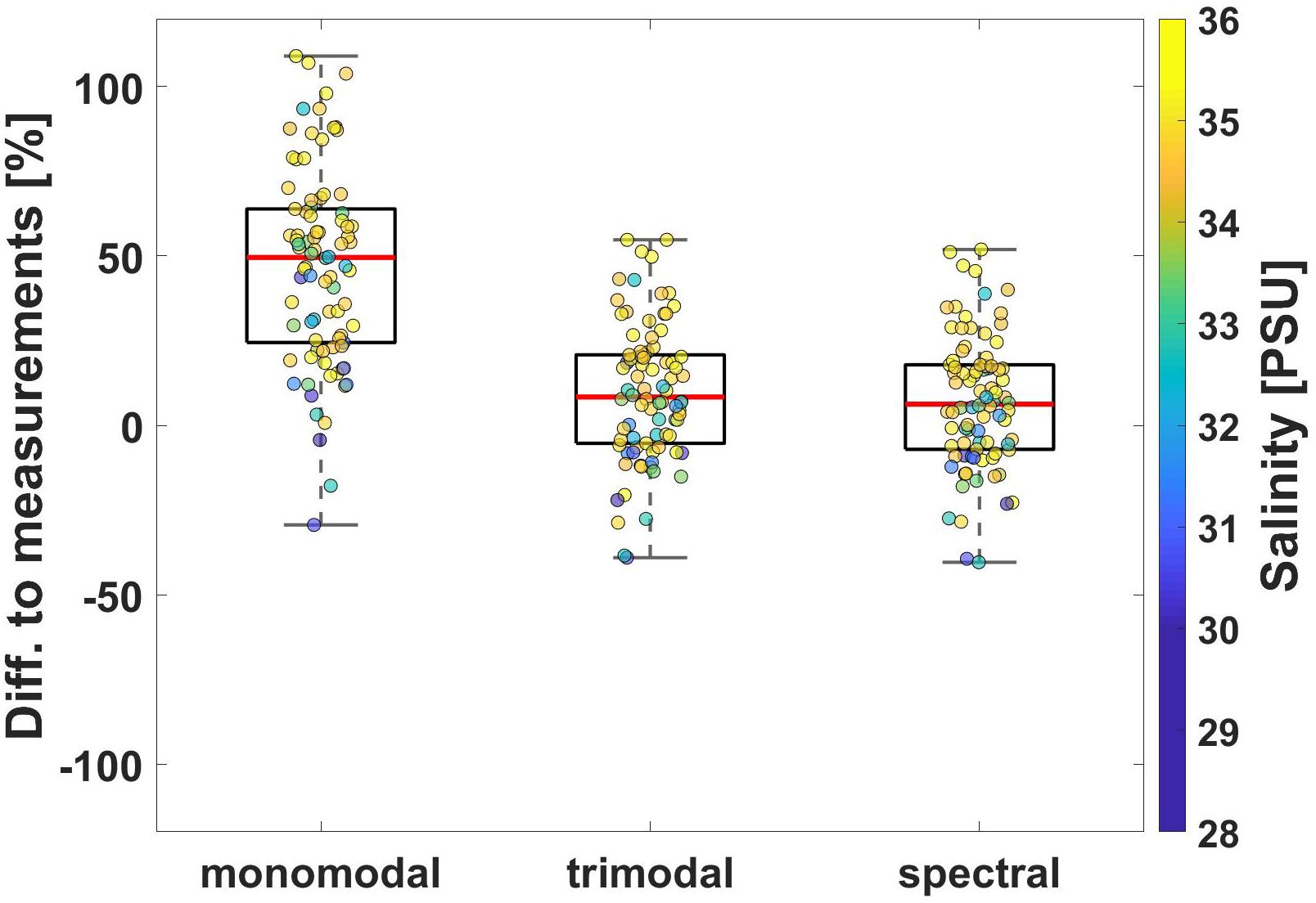
Figure 7. Boxplot of the differences between depth-integrated modeled and measured PAR as percentage of the measurements. The data points give the differences for the individual stations, colored according to the respective median salinity.

In terms of computational effort, the monomodal approach required only 12% the time of the spectral approach, while the trimodal approach was only marginally slower with 13%. Although these values can only be a rough estimate, since the computational effort always depend on the hardware used and the efficiency of the code, this finding indicates that the trimodal approach is an excellent compromise between computational efficiency and accuracy regarding PAR attenuation with depth.

This is also supported by the fact that despite the differences in depth-integrated PAR, the PAR profiles derived with the trimodal approach reproduced well common measures of water transparency, like the center and the lower limit of the euphotic zone, which correspond to the depths were 10 and 1% of surface PAR are available to photosynthetic organisms (Kirk, 2011; Figure 8). For both penetration depths, linear correlations between measured and modeled data showed high R² values (0.83 and 0.86), and the slope of the fit was near the 1:1 line in both cases. This was comparable to regressions using data obtained from the spectral model (Table 4). Also the 10 and 1% PAR penetration depths derived from the monomodal model showed a strong linear correlation to the measured depths (R² of 0.8 for both depths). The slopes deviated more from the 1:1 line than that from the trimodal and spectral dataset, but the main difference was a statistically significant (p < 0.05) offset of 3.9 m (10% depth) and 7.4 m (1% depth). This would lead to high errors in estimating water transparency, especially in shallow coastal areas.

FIGURE 8

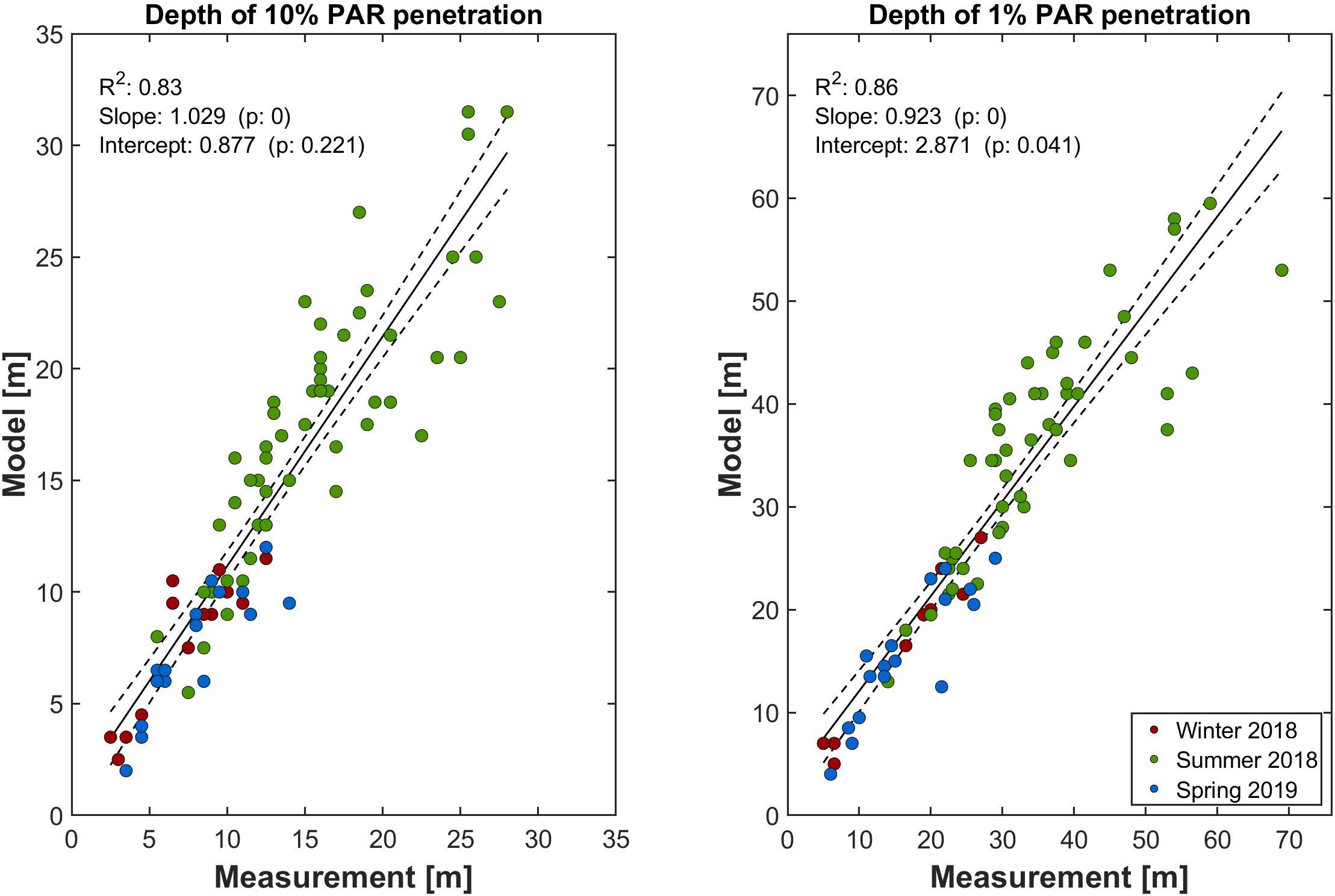
Figure 8. Comparison of penetration depths from PAR derived from in situ and modeled profiles (trimodal approach). The solid line represents the linear fit, while the dashed lines give its 95% confidence interval.

TABLE 4

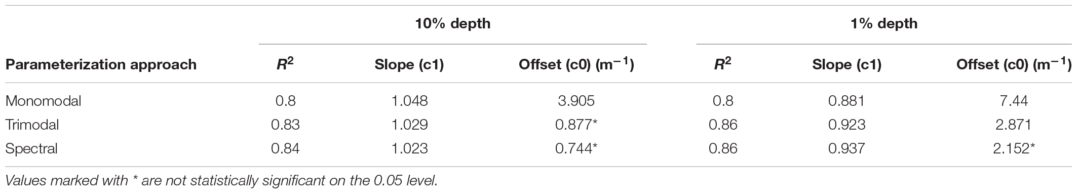
Table 4. Results of linear fits between observed and modeled PAR penetration depths for the different parameterization approaches.

Derivation of Secchi Depth From K_d (II)

A special feature of the trimodal parameterization approach is the fact that the second spectral range [K_d (II)] covers basically the wavelengths where the majority of the measured K_d spectra had their minimum (Figure 3). As the SD can be estimated by 1/K_d (λ_min) (Lee et al., 2015), in this study it was also tested to use K_d (II) for this purpose. As K_d (λ_min) was on average approximately 6% smaller than K_d (II) (calculation not shown), K_d (II) has been multiplied by 0.94 before calculating SD. The modeled SD were then compared to those measured at the cruise stations (Figure 9). There was a reasonably robust linear relationship between the data modeled on the basis of K_d (II) and the measured SD data (R² = 0.65, left panel). However, in contrast to the results shown in Lee et al. (2015), the modeled values were almost 50% higher than the observations. This was apparently not an effect from using K_d (II) for SD calculation, as the correlation with SD data modeled with the real K_d (λ_min) yielded almost identical results (data not shown). However, when only a data range of 0–10 m is considered, the slope of the linear regression is much closer to the 1:1 line. Although this could indicate inaccuracies in K_d (II) values derived with the OAS-specific K_d^∗ coefficients in clearer waters, this is probably not the case, since the estimations of 10 and 1% light penetration depths (Figure 8) do not show similar deviations at these stations. Therefore, it is more likely that there was a bias in the SD field measurements in these optically deeper waters. As SD measurements are by their nature subjective, errors can occur easily, especially when the measurements are performed near the ship under suboptimal conditions (moderate to high waves or currents that drag the disk below the vessel). Nevertheless, even if the deviations were a result of the modeling process, the correlations provided in Figure 9 would provide a mean to correct for that.

FIGURE 9

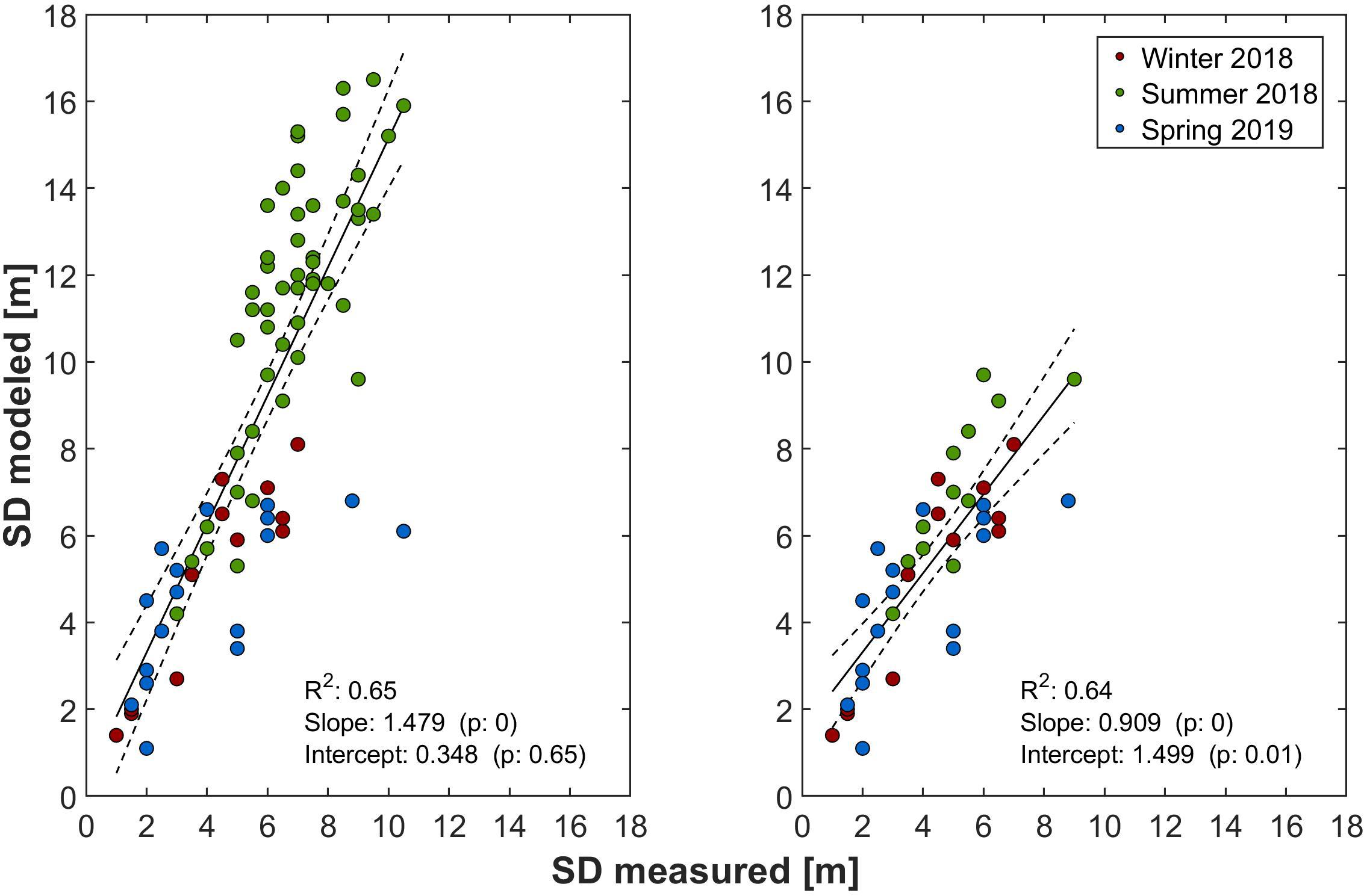
Figure 9. Correlation of observed Secchi depths and those derived from K_d in spectral region II (left). Same correlation considering only values up to 10 m depth (right). The solid line represents the linear fit, while the dashed lines give its 95% confidence interval.

Practical Implementation of the Trimodal Parameterization in Numerical Models

The implementation of the trimodal parameterization in an existing coastal model could be made comparably straightforward. Of course, the first prerequisite would be that the model provides the variables used in the parameterization to describe PAR attenuation (chl-a, salinity, and iSPM), or that they could be derived from other variables of the model. If this is the case, the old parameterization could be replaced with the trimodal approach, including the coefficients shown in Table 2. Ideally, their validity for the area of interest should be checked beforehand as they could vary due to regional and temporal differences in the properties of the OAS, as discussed before. Subsequently, PAR has to be parted proportionally to the size of the spectral bands, and each band has to be attenuated independently with depth, as stressed in section “Assessment of the Model Approaches.” Practically, this is realized in a stepwise process using the K_d (I/II/III) value calculated for this depth and the light that is transferred from the layer above as input.

The use of the trimodal parameterization in models covering both costal and open ocean waters would require additional modifications, a crucial point would be the smooth transition between case II waters, where attenuation by the different OAS vary independently, and case I waters, where they vary with phytoplankton abundance. Assuming that the trimodal approach is used for the whole area of the model, and that there is no jump between different PAR parameterizations, the calculations would be made like described above and in section “Assessment of the Model Approaches.” The attenuation due to iSPM (mostly suspended sediment), would become less anyway in the three bands toward the open ocean areas since the model would probably not provide much suspended sediments in these (usually deeper) areas. Otherwise, the suspended sediment component would have turned off in water to be considered case I, as suggested by Thewes et al. (2020). Similarly, also K_{d cdom} (which reflects the contribution of terrestrial CDOM to PAR attenuation) would become smaller, reflecting that in the more saline open ocean waters this OAS is not relevant anymore. However, according to Figure 5, K_{d cdom} would become negative at salinity >35.5, resulting in increasing (instead of decreasing) PAR with depth in the open ocean. To avoid this artifact, the model should set negative K_{d cdom} values to zero. The most crucial part is probably related to K_d^∗_phyt: due to differences in taxonomical composition, size, and the increasing importance of autochthonous CDOM, its values are probably different between the coastal and open ocean areas. In order to include such a shift in the parameterization, K_d^∗_phyt could be related to a parameter that describes the water mass or the coastal distance (e.g., salinity or bathymetry). However, this is probably not straightforward and would require additional studies specifically dedicated to this problem (including more measurements under open ocean conditions).

Conclusion

In contrast to the open ocean, where the optical properties are predominantly determined by the phytoplankton present, coastal waters are optically more complex. CDOM and non-algal particles play a more important role, and their contribution vary independently of phytoplankton abundance. However, when it comes to vertical attenuation of light (or more specific, of PAR) that is important for the calculation of primary productivity and phytoplankton growth, many biogeochemical models use parameterizations that do not account for this complexity. Furthermore, also the spectral variability in the light attenuation by different OAS is often ignored by, e.g., using mean values calculated over the whole spectrum as attenuation coefficients.

In this study, a trimodal parameterization has been developed that divides surface PAR in three parts which sizes correspond to the sizes of three spectral bands. These bands have been selected according to the spectral shape of K_d (λ) spectra measured in the field. In the first band, all OAS contribute similar to attenuation, while that of water is negligible. The second band is that where K_d had its minimum, and the third band is dominated by attenuation of water and iSPM, while contributions of CDOM and phytoplankton (chl-a) are negligible. PAR in each band is attenuated independently by using band- and substance-specific attenuation coefficients (K_d^∗) and profiles of OAS concentrations. This parameterization was compared in terms of accuracy in light attenuation and computational effort with a classical monomodal parameterization (that includes, however, in addition to chl-a also contributions of CDOM and iSPM to light attenuation), and a full spectral parameterization with 1 nm resolution. Although the K_d^∗ values in this study have been derived from a dataset that contains already a certain degree of spatial and seasonal heterogeneity, it has to be kept in mind that they can change due to changes in the OAS’ optical properties. Thus, they can be considered as a reasonable first estimate, but should be validated with additional field data, especially when the parameterization would be used in other coastal areas.

However, PAR profiles have been modeled for all approaches and were compared to field measurements of PAR. It has been found that the trimodal approach for the investigated research area of the North Sea provided an estimation of light attenuation that is of similar accuracy as a spectral approach, by being simultaneously of similar efficiency as a classical monomodal approach. Furthermore, as a special feature, the use of the trimodal approach allows the estimation of SDs that are of similar quality than those based on spectral K_d. This offers the possibility of adding SD with low effort as an output to biogeochemical models, and therefore relate model scenarios to historical observations of SD data. In summary, this makes the trimodal approach an ideal parameterization of light attenuation for biogeochemical models with many nodes, facilitating improved light prediction and primary production estimation on wide temporal and spatial scales.

Data Availability Statement

The data used in this study are available on request from the authors. Unprocessed data from the free falling profiler as well as quality controlled CTD data from all cruises are available on PANGAEA (Badewien and Wisotzki, 2018, 2019; Krock and Wisotzki, 2018; Wollschläger et al., 2020a,b,c).

Author Contributions

JW and OZ conceptualized the study. BT, DV, and JW performed the field investigations. BT and JW analyzed the data. All authors were involved in the interpretation of the results. DV, JW, and OZ wrote the manuscript. All authors contributed to the article and approved the submitted version.

Funding

This work was supported by the project “Coastal Ocean Darkening,” funded by the German Lower Saxony Ministry for Science and Culture [VWZN3175]. DFKI acknowledges financial support by the MWK through “Niedersachsen Vorab” [ZN3480].

Conflict of Interest

The authors declare that the research was conducted in the absence of any commercial or financial relationships that could be construed as a potential conflict of interest.

Acknowledgments

Thanks goes to Rohan Henkel and Kathrin Dietrich who helped with the deployments of the instruments and with the laboratory analyses. We would like to thank also Daniel Thewes for giving his comments regarding the implementation of the parameterizations in models. As well, many thanks go to the crew of the research vessel “Heincke” for their help on the cruises AWI_HE503_00, AWI_HE516_00, and AWI_HE527_00 where the data for this study has been gathered. Finally, we would like to thank the reviewers of this manuscript who helped to improve its quality by their comments.

Supplementary Material

The Supplementary Material for this article can be found online at: https://www.frontiersin.org/articles/10.3389/fmars.2020.00512/full#supplementary-material

References

Arar, E. J., and Collins, G. B. (1997). Method 445.0: In Vitro Determination of Chlorophyll a and Pheophytin a in Marine and Freshwater Algae by Fluorescence. Ohio: National Exposure Research Laboratory.

Google Scholar

Babin, M., and Stramski, D. (2002). Light absorption by aquatic particles in the near-infrared spectral region. Limnol. Oceanogr. 47, 911–915. doi: 10.4319/lo.2002.47.3.0911

CrossRef Full Text | Google Scholar

Badewien, T. H., and Wisotzki, A. (2018). Physical Oceanography During HEINCKE cruise HE503. Bremerhaven: Alfred Wegener Institute.

Google Scholar

Badewien, T. H., and Wisotzki, A. (2019). Physical Oceanography During HEINCKE cruise HE527. Bremerhaven: Alfred Wegener Institute.

Google Scholar

Bowers, D. G., and Binding, C. E. (2006). The optical properties of mineral suspended particles: A review and synthesis. Estuar. Coast. Shelf Sci. 67, 219–230. doi: 10.1016/j.ecss.2005.11.010

CrossRef Full Text | Google Scholar

Bowers, D. G., Evans, D., Thomas, D. N., Ellis, K., and Williams, P. J. L. B. (2004). Interpreting the colour of an estuary. Estuar. Coast. Shelf Sci. 59, 13–20. doi: 10.1016/j.ecss.2003.06.001

CrossRef Full Text | Google Scholar

Bricaud, A., Babin, M., Morel, A., and Claustre, H. (1995). Variability in the chlorophyll-specific absorption coefficients of natural phytoplankton: Analysis and parameterization. J. Geophys. Res. 100, 13321–13332.

Google Scholar

Bricaud, A., Claustre, H., Ras, J., and Oubelkheir, K. (2004). Natural variability of phytoplanktonic absorption in oceanic waters: Influence of the size structure of algal populations. J. Geophys. Res. Ocean. 109:CI1010.

Google Scholar

Clementson, L. A., and Wojtasiewicz, B. (2019). Dataset on the absorption characteristics of extracted phytoplankton pigments. Data Br. 24:103875. doi: 10.1016/j.dib.2019.103875

PubMed Abstract | CrossRef Full Text | Google Scholar

Cunningham, A. (1996). Variability of in-vivo chlorophyll fluorescence and its implications for instrument development in bio optical oceanography. Sci. Mar. 60, 309–315.

Google Scholar

Dutkiewicz, S., Hickman, A. E., Jahn, O., Gregg, W. W., Mouw, C. B., and Follows, M. J. (2015). Capturing optically important constituents and properties in a marine biogeochemical and ecosystem model. Biogeosciences 12, 4447–4481. doi: 10.5194/bg-12-4447-2015

CrossRef Full Text | Google Scholar

Fasham, M. J. R., Ducklow, H. W., and McKelvie, S. M. (1990). Modeling plankton dynamics in oceanic mixed systems. J. Mar. Res. 48, 591–639. doi: 10.1357/002224090784984678

CrossRef Full Text | Google Scholar

Helms, J. R., Stubbins, A., Ritchie, J. D., Minor, E. C., Kieber, D. J., and Mopper, K. (2008). Absorption spectral slopes and slope ratios as indicators of molecular weight, source, and photobleaching of chromophoric dissolved organic matter. Limnol. Oceanogr. 53, 955–969. doi: 10.4319/lo.2008.53.3.0955

CrossRef Full Text | Google Scholar

Holinde, L., and Zielinski, O. (2016). Bio-optical characterization and light availability parameterization in Uummannaq Fjord and Vaigat-Disko Bay (West Greenland). Ocean Sci. 12, 117–128. doi: 10.5194/os-12-117-2016

CrossRef Full Text | Google Scholar

Kiefer, D. A. (1973). Chlorophyll a fluorescence in marine centric diatoms: Responses of chloroplasts to light and nutrient stress. Mar. Biol. 23, 39–46. doi: 10.1007/bf00394110

CrossRef Full Text | Google Scholar

Kirk, J. T. (1997). Point-source integrating-cavity absorption meter: theoretical principles and numerical modeling. Appl. Opt. 36, 6123–6128.

Google Scholar

Kirk, J. T. O. (2011). Light & Photosynthesis in Aquatic Ecosystems, 3rd Edn. New York, NY: Cambridge University Press.

Google Scholar

Knust, R., Nixdorf, U., and Hirsekorn, M. (2017). Research Vessel HEINCKE Operated by the Alfred-Wegener-Institute. J. Large-Scale Res. Facil. JLSRF 3, 1–8.

Google Scholar

Krock, B., and Wisotzki, A. (2018). Physical Oceanography During HEINCKE cruise HE516. Bremerhaven: Alfred Wegener Institute.

Google Scholar

Kühn, W., and Radach, G. (1997). A one-dimensional physical-biological model study of the pelagic nitrogen cycling during the spring bloom in the northern North Sea (FLEX ’76). J. Mar. Res. 55, 687–734. doi: 10.1357/0022240973224229

CrossRef Full Text | Google Scholar

Lee, Z., Shang, S., and Stavn, R. (2018). AOPs are not additive: on the biogeo-optical modeling of the diffuse attenuation coefficient. Front. Mar. Sci. 5:8. doi: 10.3389/fmars.2018.00008

CrossRef Full Text | Google Scholar

Lee, Z.-P., Du, K.-P., and Arnone, R. (2005). A model for the diffuse attenuation coefficient of downwelling irradiance. J. Geophys. Res. 110:C02016.

Google Scholar

Lee, Z. P., Shang, S., Hu, C., Du, K., Weidemann, A., Hou, W., et al. (2015). Secchi disk depth: A new theory and mechanistic model for underwater visibility. Remote Sens. Environ. 169, 139–149. doi: 10.1016/j.rse.2015.08.002

CrossRef Full Text | Google Scholar

Liss, P. S. (1976). “Conservative and non-conservative behavior of dissolved constituents during estuarine mixing,” in Estuarine Chemistry, eds J. D. Burton and P. S. Liss (London: Academic Press), 93–130.

Google Scholar

Mascarenhas, V. J., Voß, D., Wollschläger, J., and Zielinski, O. (2017). Fjord light regime: Bio-optical variability, absorption budget, and hyperspectral light availability in Sognefjord and Trondheimsfjord, Norway. J. Geophys. Res. Ocean. 122.

Google Scholar

McFarland, W. N. (1986). Light in the sea - correlations with behaviors of fishes and invertebrates. Integr. Comp. Biol. 26, 389–401. doi: 10.1093/icb/26.2.389

CrossRef Full Text | Google Scholar

Mobley, C. D. (1994). Light and Water: Radiative Transfer in Natural Waters. Cambridge, MA: Academic press.

Google Scholar

Mobley, C. D., Chai, F., Xiu, P., and Sundman, L. K. (2015). Impact of improved light calculations on predicted phytoplankton growth and heating in an idealized upwelling-downwelling channel geometry. J. Geophys. Res. Ocean. 120, 875–892. doi: 10.1002/2014jc010588

CrossRef Full Text | Google Scholar

Morel, A. (1988). Optical modelling of upper ocean in relation to its Biogenic Matter content (case 1 waters). J. Geophys. Res. 93, 10749–10769.

Google Scholar

Morel, A., and Bricaud, A. (1981). Theoretical Results Concerning Light-Absorption in a Discrete Medium, and Application To Specific Absorption of Phytoplankton. Deep. Res. Part A Oceanogr. Res. Pap. 28, 1375–1393. doi: 10.1016/0198-0149(81)90039-x

CrossRef Full Text | Google Scholar

Morel, A., and Maritorena, S. (2001). Bio-optical properties of oceanic waters: A reappraisal. J. Geophys. Res. Ocean. 106, 7163–7180. doi: 10.1029/2000jc000319

CrossRef Full Text | Google Scholar

Morel, A., and Prieur, L. (1977). Analysis of variations in ocean color. Limnol. Oceanogr. 22, 709–722. doi: 10.4319/lo.1977.22.4.0709

CrossRef Full Text | Google Scholar

Mueller, J. L., Fargion, G. S., Mcclain, C. R., Morel, A., Frouin, R., Davis, C., et al. (2003). Ocean Optics Protocols For Satellite Ocean Color Sensor Validation, Revision 4, Volume III?: Radiometric Measurements and Data Analysis Protocols NASA / TM-2003- Ocean Optics Protocols For Satellite Ocean Color Sensor Validation, Revision 4, Volume II. Ocean Color web page III. Washington, DC: NASA, 84.

Google Scholar

Organelli, E., Claustre, H., Bricaud, A., Schmechtig, C., Poteau, A., Xing, X., et al. (2016). A novel near-real-time quality-control procedure for radiometric profiles measured by bio-argo floats: Protocols and performances. J. Atmos. Ocean. Technol. 33, 937–951. doi: 10.1175/jtech-d-15-0193.1

CrossRef Full Text | Google Scholar

Paulson, C. A., and Simpson, J. J. (1977). Irradiance Measurements in the Upper Ocean. J. Phys. Oceanogr. 7, 952–956. doi: 10.1175/1520-0485(1977)007<0952:imituo>2.0.co;2

CrossRef Full Text | Google Scholar

Röttgers, R., and Doerffer, R. (2007). Measurements of optical absorption by chromophoric dissolved organic matter using a point-source integrating-cavity absorption meter. Limnol. Oceanogr. Methods 5, 126–135. doi: 10.4319/lom.2007.5.126

CrossRef Full Text | Google Scholar

Röttgers, R., Häse, C., and Doerffer, R. (2007). Determination of the particulate absorption of microalgae using a point-source integrating-cavity absorption meter. Limnol. Oceanogr. Methods 5, 1–12. doi: 10.4319/lom.2007.5.1

CrossRef Full Text | Google Scholar

Röttgers, R., Schönfeld, W., Kipp, P.-R., and Doerffer, R. (2005). Practical test of a point-source integrating cavity absorption meter: the performance of different collector assemblies. Appl. Opt. 44, 5549–5560.

Google Scholar

Smith, R. C., and Baker, K. S. (1984). “The analysis of ocean optical data,” in Ocean Optics VII, ed. M. A. Blizard (Washington, DC: SPIE), 119–126.

Google Scholar

Smith, R. C., and Baker, K. S. (1986). “Analysis of ocean optical data II,” in Ocean Optics VIII, ed. M. A. Blizard (Washington, DC: SPIE), 95–107.

Google Scholar

Soohoo, J. B., Kiefer, D. A., Collins, D. J., and Mcdermid, I. S. (1986). In vivo fluorescence excitation and absorption spectra of marine phytoplankton: I. Taxonomic characteristics and responses to photoadaptation. J. Plankton Res. 8, 197–214. doi: 10.1093/plankt/8.1.197

CrossRef Full Text | Google Scholar

Stedmon, C. A., and Markager, S. (2003). Behaviour of the optical properties of coloured dissolved organic matter under conservative mixing. Estuar. Coast. Shelf Sci. 57, 973–979. doi: 10.1016/s0272-7714(03)00003-9

CrossRef Full Text | Google Scholar

Thewes, D., Stanev, E. V., and Zielinski, O. (2020). Sensitivity of a 3D Shelf Sea Ecosystem Model to Parameterizations of the Underwater Light Field. Front. Mar. Sci. 6:816. doi: 10.3389/fmars.2019.00816

CrossRef Full Text | Google Scholar

Wollschläger, J., Henkel, R., Voß, D., and Zielinski, O. (2020a). Hyperspectral Underwater Light Field Measured During the Cruise HE503 with RV HEINCKE. Bremerhaven: Alfred Wegener Institute.

Google Scholar

Wollschläger, J., Henkel, R., Voß, D., and Zielinski, O. (2020b). Hyperspectral Underwater Light Field Measured During the cruise HE527 with RV HEINCKE. Bremerhaven: Alfred Wegener Institute.

Google Scholar

Wollschläger, J., Henkel, R., Voß, D., and Zielinski, O. (2020c). Hyperspectral Underwater Light Field Measured during the cruise HE516 with RV HEINCKE. Bremerhaven: Alfred Wegener Institute.

Google Scholar

Wollschläger, J., Röttgers, R., Petersen, W., and Zielinski, O. (2019). Stick or Dye: Evaluating a Solid Standard Calibration Approach for Point-Source Integrating Cavity Absorption Meters (PSICAM). Front. Mar. Sci. 5:534. doi: 10.3389/fmars.2018.00534

CrossRef Full Text | Google Scholar

Zielinski, O. (2013). Subsea Optics: An Introduction, Subsea Optics and Imaging. Sawston: Woodhead Publishing Limited.

Google Scholar

Zielinski, O., Llinás, O., Oschlies, A., and Reuter, R. (2002). Underwater light field and its effect on a one-dimensional ecosystem model at station ESTOC, north of the Canary Islands. Deep. Res. Part II Top. Stud. Oceanogr. 49, 3529–3542. doi: 10.1016/s0967-0645(02)00096-6

CrossRef Full Text | Google Scholar