Diving Behavior of Mirounga leonina: A Functional Data Analysis Approach

Introduction

In a global warming context, studying and understanding the foraging behavior of predators and their relationships with their surrounding environment is fundamental for conservation and management programs (Runge et al., 2014). According to optimal foraging theory, individuals are expected to minimize the time spent searching for and capturing food while maximizing their energy intake (Stephens and Krebs, 1986). Aquatic predators, such as birds, reptiles, and mammals that feed underwater but must breathe at the surface, are expected to optimize their capture success within the constraints of oxygen availability (Kooyman, 2012). For 20 years, the behavior of these specific animals has been widely studied with the implementation of tags that allow the sampling of numerous data both on their dive behavior, their physiology, and their biological and physical surrounding environment. Nowadays, bio-logging devices are the most appropriate tools to provide critical information on the diving and foraging of free-ranging animals (Evans et al., 2013). Technological advances have led to size and weight reduction of autonomous devices with gains in battery lifetime and memory size as well as new variables monitored. This emergence of new data sampled at high frequency (Block et al., 2011) enables the study of diving behaviors at various scales in time and space (Jonsen et al., 2007; Scheffer et al., 2012; Nowacek et al., 2016). Time Depth Recorders (TDRs) provide a large amount of data that are downloaded from sensors to computer systems where they are stored. In addition, many of these tags also sample environmental data (Harcourt et al., 2019). Despite concrete advances in the study of foraging behavior, a gap remains between fast advances in sampling technologies and adapted methods of data analysis required to face the increase in data complexity. Technological innovation and development of new measuring devices are much faster than the invention and validation of new methods for operational data processing. It is because innovative methods are often unknown to the scientists who build up the sampling design but also because the required methods are not yet available. New data leads, indeed, to problems that no one had ever thought of. Besides, many tags require on-board processing for satellite data transmission (Fedak et al., 2002). Energy costs impose constraints in this on-board processing to reduce computational time and to improve the quality of transmitted data while minimizing the amount of transmitted information. It is therefore necessary to have access to adapted methods to find the best compromises to satisfy these constraints.

One example of this fast increase is the biologging data volume provided by the long term monitoring of the deep and continuously diving southern elephant seal (Mirounga leonina) in the Southern Ocean as part of the National Observatory System MEMO (Mammals as Ocean Samplers) (Harcourt et al., 2019) or as a part of the Marine Mammals Exploring the Oceans Pole to Pole MEOP consortium (Treasure et al., 2017). These animals are equipped with a TDR tag and/or with a conductivity–temperature–depth Satellite Relay Data Logger (CTD-SRDL) tag measuring time-depth profiles (subsequently referred to as “SRDL”). Large numbers of deployments have given rise to large databases that provide access to sampled oceanographic variables (temperature, salinity, and fluorescence profiles) as well as movements of equipped individuals, especially dives (Fedak et al., 2001; Roquet et al., 2014).

Figure 1 displays an example of time-depth dive profiles of southern elephant seals, Mirounga leonina. During offshore periods lasting 3–7 months, a female elephant seal performs quasi-continuous long deep dives (26min in average, 432m deep) punctuated by short breathing episodes at the surface (Hindell et al., 2016). The availability of high-frequency data combined with this continuous aspect of the dives lead us to consider that dives can be handled as curves. Data that arrive as observed curves are called functional data because they are observations of a variable (depth) indexed over a continuum (time). Time-depth dive profiles share common features:

• They start from the surface and end at the surface.

• The ending time and maximum depth are different between two dives.

• An observed dive is constituted with numerous sampled points.

• The number of sampled points changes between two dives.

• The sampled grid might not be equally spaced in time.

• Random errors may occur (e.g., time-depth sensor problems).

• An elephant seal can achieve several thousands of dives.

FIGURE 1

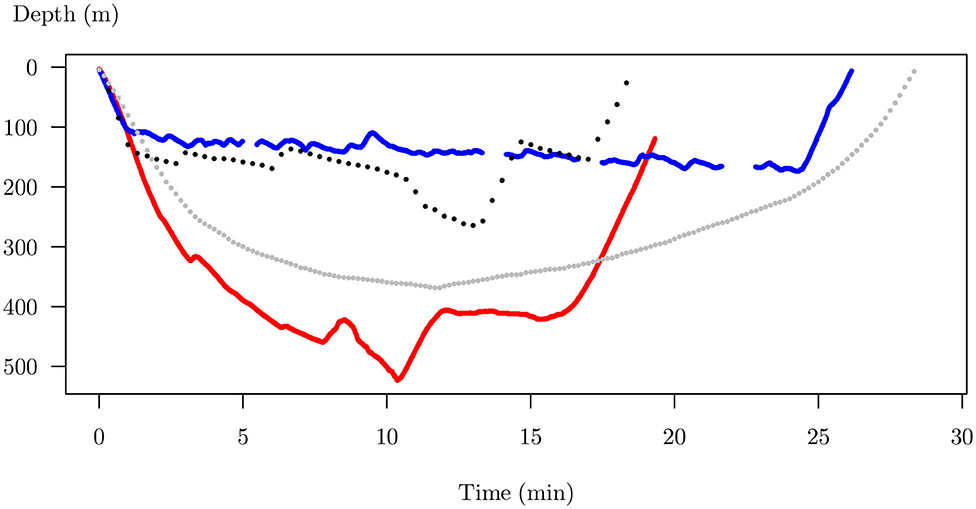
Figure 1. Four dive examples from Mirounga leonina. Each dive is plotted as depth vs. time. These dives are functional data because the variable of interest (depth) is a function of time. Dives have different length in depth and time. The number and the position of the sampled points are different. Random errors can occur due to time-depth sensor problems. In this raw form, it is impossible to compare their shape.

In their raw form, it is almost impossible to compare different dive shapes and even less to identify a small number of specific foraging behaviors.

Many studies deal with dive classification methods to organize dives in meaningful categories (Hindell et al., 1991; Campagna et al., 1995; Dragon et al., 2012). Classically, a finite set of descriptors, such as mean and maximum depth, duration of the descent, ascent, and bottom phases of the dive (see Hindell et al., 1991; Le Boeuf et al., 1993; Tremblay and Cherel, 2000; Watwood et al., 2006), are extracted from the high-frequency sampled dive data. These descriptors allow the construction of a table of observations and variables (the descriptors) over which standard multivariate analyses, such as reduction dimension methods (i.e., PCA), classification, or statistical tests (e.g., Random Forest, Thums et al., 2008; HMM, Ngô et al., 2019) will be performed. This work proposes that we study the diving behavior of Mirounga leonina through the shape comparison of time-depth dive curves without the use of predefined numerical descriptors. Indeed, the choice of the descriptors relies on empirical and historical knowledge of the diving behaviors. Here, we argue that if the option of a finite number of well-suited descriptors is the predominant method to compare a collection of dives, it remains a partial description of the entire shape of the sampled curves. We assume that shape potentially contains all the possible descriptors of a dive curve. Therefore, this work first aims at comparing dive shape and numerical descriptors. In a second step, identified shape patterns in dive profiles will be connected with prey capture events to better understand foraging behaviors and the structure of the surrounding prey field.

After that, the document introduces the data obtained from southern elephant seal tags. In a second step, technical points for the transformation of discrete data to continuous functions are presented. We then propose some dimension reduction and classification methods adapted to data that are curves to compare and to characterize diving behaviors. A comparison with classical descriptor-based methods and tests for robustness is achieved with simulations on downsampled data. The ecological relevance of the results is finally discussed by comparing the characteristic shape to the number of prey capture events. The different steps of the method used in the article are summarized in Figure 2.

FIGURE 2

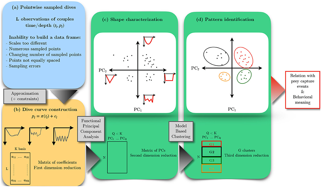
Figure 2. Workflow of functional data analysis for the study of diving behavior of Mirounga leonina. Time-depth sampled profiles (a) can be approximated with continuous curves by a linear combination of K known functions (b). This first step reduces the dimensionality of the initial data and provides a new data frame. Observations are projected with PCA in a space of small dimensions using a number Q of principal component scores. Each component reflects a specific deformation of the shape of curves (c). By construction, deformations are independent, and their magnitude can be ordered according to a percentage of explained variance. PCA scores are used as inputs for model-based clustering in order to identify characteristic shapes of sampled curves (G1, G2, G3, and G4) (d).

Materials and Methods

Processed Data

A total of 17 post-breeding southern elephant seal females, Mirounga leonina were tagged. Fieldwork was conducted at the Kerguelen Islands (Figure 3), from November to January 2010–2011 for three females, 2014–2015 for the six females, 2015–2016 for four females, and 2017–2018 for the four others. The seals were equipped with a TDR (Mk10, Wildlife Computer) recording time and depth at 0.5 or 1 Hz. For twelve females, the TDR was combined with an accelerometer. TDR-accelerometers sampled accelerations on three axes. The acceleration measured simultaneously on these three axes was used to estimate prey capture attempts (Viviant et al., 2010). Animals were captured and anesthetized using a 1:1 combination of tiletamine and zolazepam (Zoletil 100), which was injected intravenously (McMahon et al., 2000). After cleaning the fur with acetone, data loggers were glued on the head of the seals, using quick-setting epoxy (Araldite AW 2101). Therefore, the data loggers collected N = 87, 691 dives (Figure 1). All fieldwork activities were approved by TAAF (French Antarctic and sub-Antarctic Territories) Ethic committee (Comité Environnement et Préfet des Terres Australes et Antarctiques Françaises). All effort was made to minimize handling time.

FIGURE 3

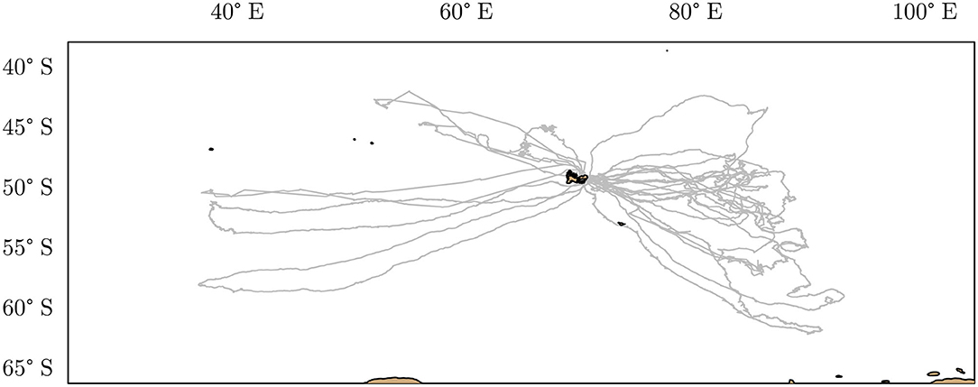
Figure 3. Post-breeding foraging trips around the Kerguelen Islands of 17 female southern elephant seals equipped between October 2010 and October 2017 (gray lines). The coastline's contours are indicated in black, and land areas are in brown.

Dive Curve Construction

Let us consider a sampled dive. Data arrive as a collection of L pairs (t₁, p₁), ⋯ , (t_L, p_L) where t_l is time (min), and p_l the observed depth (m). We suppose that an observation p_l of the diving depth at time t_l may be well-represented by a continuous function π of time such that:

$\begin{array}{l}{p}_l=\pi (t_l)+{\epsilon }_l\end{array}$

where π is the deterministic part of the dive, and ε is a remainder. If the function π is well-chosen, it is hoped that this remainder is as small as possible. The form of π, which is directly connected to the shape of the dive, is expressed as a linear combination of K known basis functions ϕ₁, ⋯ , ϕ_K such that

$\begin{array}{l}\pi (t)={\alpha }_1{\varphi }_1(t)+{\alpha }_2{\varphi }_2(t)+\cdots +{\alpha }_K{\varphi }_K(t).\end{array}$

The basis functions ϕ_k are chosen by the practitioner and are continuous functions of time. The shape of the function π is entirely determined by the knowledge of the coefficients α₁, ⋯ , α_K which are estimated using the data (t₁, p₁), ⋯ , (t_L, p_L) by penalized least squares regression (see Supplementary Material).

This regression procedure is influenced by the following:

• the choice of the very nature of the basis (i.e., Fourier basis, B-splines basis, and polynomial basis);

• the choice of the number K of basis functions (i.e., the number of coefficients); and

• the choice of additional constraints suggested by the data (or by some knowledge of the practitioner).

Many choices for basis functions are possible. Fourier basis, polynomial basis, splines, wavelets may be used. However, the choice for the basis has little influence for describing the shape of a dive (Ramsay and Silverman, 2005). In our case, cubic B-splines basis (piecewise polynomials of degree 3) is the most advisable choice as it combines fast computation capabilities and flexibility. This is a critical point for the onboard processing of data in satellite relayed data loggers.

Although a small number K < L of basis functions is generally sufficient to capture the main variations in the shape of any dive, the choice of this number may have a significant influence on the shape of the estimated curves. The bigger K is, the closer the fit will be to the data, as usual in a regression problem (Figure 4).

FIGURE 4

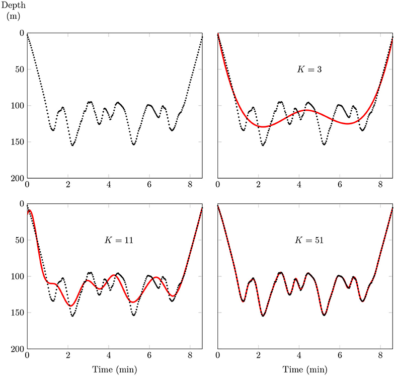
Figure 4. An example of data fitting using a B-spline basis. The dotted line is a sample of a dive (259 sampling location), and the red line is the fitting curve. As the number K of basis functions increases, the quality of the fit is improved.

However, the penalized regression procedure allows for getting rid of this choice by giving a compromise between the regularity of the obtained curve and its closeness to the data. This particular point will be illustrated in detail in the Result section.

Finally, a more detailed look at the data suggests that additional constraints must be included when searching for the best fit. Due to 0-offset correction, each dive starts from the surface [i.e., (t₁, p₁) = (0, 0)], and ends at the surface [i.e., (t_L, p_L) = (t_M, 0) where t_M is the duration of the dive]. The B-spline must reach the surface at least at the beginning and at the end of a dive, which does not occur with a non-constrained regression procedure. One other advantage of using penalized B-splines is that it is easy to include some additional pointwise constraints while keeping a simple solution to the regression problem (Ramsay and Silverman, 2005). These constraints can take various forms, especially if the curve must go through some points or if the derivative of the curve must have some values on some particular points (see Supplementary Material).

Shape is all the geometrical information that remains when location, scale, and rotation effects are filtered out from an object (Dryden and Mardia, 2016). Therefore, the comparison between several diving shapes imposes that every estimated curves must start and finish at the same diving time. It is not the case as the diving time changes from dive to dive (Figure 1). In the same way, the shape of each curve must be independent of their maximum dive. These differences arise from physical and/or biological factors (prey density, frontal area, body condition). As shown in Figure 5, if care is taken to normalize diving curves by reducing both time and depth range to segment [0, 1], very different dives get the same shapes, which might highlight similar behaviors. Sampled data are then normalized before B-splines are computed, as shown in Figure 5.

FIGURE 5

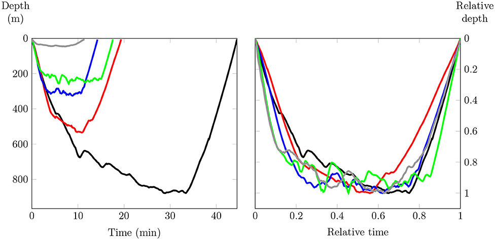
Figure 5. On the left, the representation of some dives (raw data). On the right, the representation of the same dives after normalization. Dives have different maximum depth, different duration, but dive patterns are similar.

Principal Component Analysis of Functional Data

Starting from the estimated curves π₁, ⋯ , π_N constructed as above, the aim is now to compare the shape of dives to identify a small number of dive patterns. The high number (N = 87, 691) of observed curves makes this task not easy. We propose the use of a functional PCA adapted to data that arrive as curves (FPCA). The PCA is similar to that performed on a data table crossing N individuals (the dives) and P variables except that variables are now B-splines coefficients (Ramsay and Silverman, 2005). In that case, the PCA loadings are curves instead of vectors (eigenfunctions instead of eigenvectors). The scores of FPCA allows representing observations that are curves in a space of small dimension. Finally, observations can be reconstituted in this space of small dimensions as a linear combination between some factors of variability (the eigenfunctions) and the scores according to a given amount of variability (see Supplementary Material).

Clustering

Characteristic curve clusters are identified with classification methods. Heuristic analyses of classical use (hierarchical clustering, k-means) may be a problem when determining the number of classes and when handling outliers (Melnykov and Maitra, 2010).

Model-based clustering (MBC) is a possible alternative to find a reasonable number of clusters and to deal with outliers. The idea behind MBC is that the sample of observations (dive profiles) arises from a distribution that is a mixture (a linear combination) of several components. Each of these components is associated with a distribution function and an associated proportion in the mixture. In general, it is supposed that the distribution is gaussian multivariate. A cluster will be characterized by the parameters of the distributions (mean and variance) and by the weight (the proportion) associated with this distribution. The estimation of both distribution parameters and mixture probabilities is achieved by the expectation-maximization (EM) algorithm for maximum likelihood (Fraley and Raftery, 2002). The most suitable model and the number of clusters are determined using Integrated Complete-data Likelihood (Biernacki et al., 2000).

Moreover, MBC associates a measure of uncertainty when assigning an observation (a dive) to a given cluster. Observations detected as outliers are those for which the probability of belonging to any cluster is low, such as giving birth to a cluster of outliers. Notice that computational time is dependent on the dimension of the observations (K) and can be very expensive. One way to circumvent this problem is to achieve classification in the space of the first Q < K principal components of the FPCA, accounting for a sufficient amount of variability (let's say 90%).

Evaluation of the Robustness of the Approach

With remote sampled data, it often happens that the retrieved data are corrupted due to time-depth sensor problems. It can also happen that when tags are not recovered only a few points per dives are obtained by satellite transmission (Boehme et al., 2009). It raises several critical issues on the use of incomplete profiles, on how much results change when using downsampled data. Functional data analysis provides meaningful solutions to those problems.

The scores of an FPCA provide a useful pointwise representation of the relationships between observations that are curves. Test for robustness of Functional Data Analysis (FDA) is conducted with the following method. First, dive profiles are constructed using the whole set of observations, as described in section 1.2Dive Curve Construction. A reference FPCA is then achieved (see section Principal Component Analysis of Functional Data1.3). Next, successive downsampling steps are performed by randomly removing an increasing number of pairwise observations (t, p), and dive profiles are re-estimated. Going through this process will modify the shape of the estimated dive profiles at each step. Comparing scores of successive FPCAs conducted on modified samples will help in understanding to which extent internal relationships between observations are changed. We place the downsampling step in the worst case to test the robustness of our method. One can also proceed by downsampling on a regular grid, which will lead to similar results.

In the same way, a reference PCA is achieved using the set of discrete descriptors computed on the raw non-normalized dive data: maximum depth, dive duration, bottom time duration, descent and ascent speed and the vertical sinuosity in the bottom phase (as in Hindell et al., 1991; Le Boeuf et al., 1993; Tremblay and Cherel, 2000; Watwood et al., 2006). The discrete descriptors are also computed when downsampling the raw data, and PCAs are achieved to compare the effects of sample modifications. In both cases (FPCA and standard PCA), each raw dive is damaged by removing a proportion of random points ranging from 20 to 90% of the available data.

One way to measure the deviation from the scores of the successive FPCA (resp. PCA scores) configurations to the scores of the reference FPCA (resp. PCA scores) configuration is to compute a distance between point clouds using the same number of relevant principal components. Because of the properties of any PCA, and thus FPCA, the sign of axes can be different from one FPCA to another. It is not advisable to compare separate FPCA coordinates straightforwardly. An appropriate distance is computed by keeping the reference configuration fixed and matching the others. This technique is termed Procrustes registration in the literature (Krzanowski, 2000). Once the Procrustes registration achieved, Krzanowski distance (Krzanowski, 2000) is computed between the reference FPCA and successive FPCAs on downsampled data using a fixed number of principal components accounting for a given amount of the variability (say 90%). This distance is also computed between the reference PCA on discrete descriptors and successive PCAs on downsampled data using the same number of principal components. Krzanowski distances must be normalized to compare the results obtained with FPCAs to those with PCAs. This normalization is obtained by dividing each FPCA (or PCA) scores by the entire variance of the corresponding point cloud. It reduces the variance (sum of squares of the PCA scores) of each obtained point cloud to the unit value (see Supplementary Material).

Results

Choosing the Number K of Basis Functions

As previously mentioned (section 1.2Dive Curve Construction), the choice of the number K of basis functions may influence the accuracy of the fits when constructing curves from raw data. The larger K, the better data are fitted, but the fit may also include some noise or spurious local variations. On the other hand, if K is too small, some essential features of the curve can be missed (Figure 4). The choice of an optimal value of K is achieved using the same idea as to test the robustness of the FDA approach (section 1.5Evaluation of the Robustness of the Approach). First, a reference FPCA is carried out using a great number K = 50 of basis functions. The idea is now to achieve FPCAs on curves fitted when decreasing the number K to check in which extent internal relationships between observations are modified. The Krzanowski distance is computed by keeping the reference FPCA fixed and matching the others.Figure 6 displays variations of the distance between the reference FPCA configuration (K = 50) and other FPCAs when increasing the number K of basis functions. The first five principal components of each FPCA accounts for about 90% of the variability (88.2±4.3%).

FIGURE 6

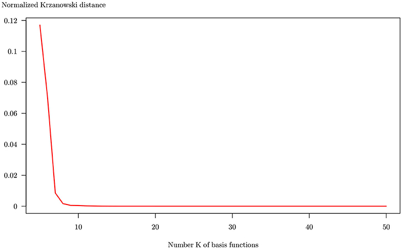
Figure 6. Krzanowski distance computed between reference FPCA (K = 50 basis functions) and FPCAs with K ranging from 5 to 50. Distances are computed using five principal components, accounting for about 90% of the entire variability in every case.

The Krzanowski distance is rapidly decreasing and vanishes to zero for K≥8 of basis functions. It means that using more than eight basis functions has a few effects on the internal relationships between observations. For the following, an arbitrary number K = 20 is chosen as a reasonable number of basis functions.

Summary Statistics

Classical summary statistics can also be computed when considering data as curves. Figure 7A displays the mean curve given with

$\begin{array}{l}\bar{\pi }(t)=\frac{1}{N}{\displaystyle \sum _{n=1}^N}{\pi }_n(t)\end{array}$

where N is the number of sampled dives, and the standard deviation function computed with

$\begin{array}{l}{\sigma }^2(t)=\frac{1}{N}{\displaystyle \sum _{n=1}^N}\left[{\pi }_n(t)-\bar{\pi }(t)\right].\end{array}$

Mean dive gets a symmetrical U-shape with a maximum depth at 0.8 (Figure 7A). When normalized, the maximum depth of each curve is 1. The mean curve of a set of dives with varying maximum depth (in time and magnitude) cannot reach a depth of 1. In the same way, the shape of the standard deviation function can be split into three parts: descent, bottom, and ascent phase. An increasing shape variability is observed during the descent. The bottom phase or bottom behavior phase is characterized by an equal vertical depth variability around 0.2, and this variability decreases with the ascent. As all dive curves start and finish at the surface, the variability vanishes to zero close to the surface. One can also use the correlation bivariate function

$\begin{array}{l}cor{r}_N(t,s)=\frac{1}{N}{\displaystyle \sum _{n=1}^N}\left(\frac{{\pi }_n(t)-\bar{\pi }(t)}{\sigma (t)}\right)\left(\frac{{\pi }_n(s)-\bar{\pi }(s)}{\sigma (s)}\right)\end{array}$

to summarize the dependency of records across different values of normalized time.

FIGURE 7

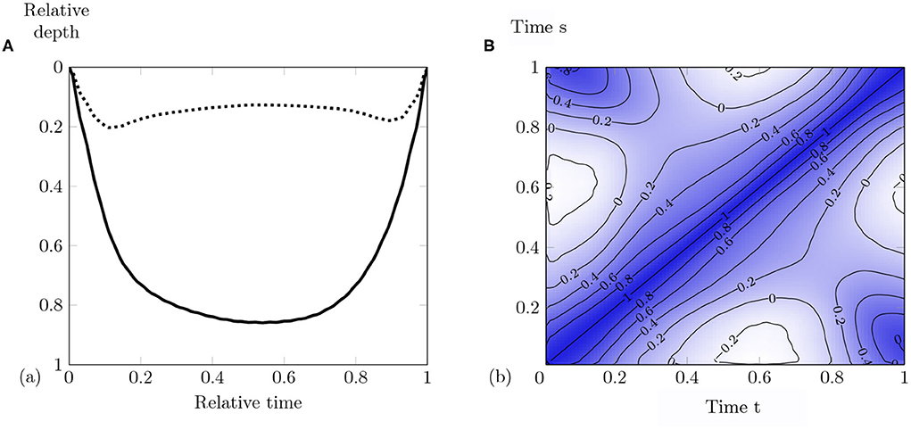
Figure 7. (A) Mean dive (solid curve) and standard deviation function (dotted curve). (B) Contour plot of the correlation corr_N(t, s) computed on the entire set of coefficients of the B-splines expansion of the normalized dives. This bivariate function is symmetrical as a correlation matrix. It shows the correlation of normalized dives for each couple of times (t, s). For example, the correlation between the beginning of dives (s = 0.05) and dives at t = 0.6 is minimum (−0.25). Correlation scale from −0.25 (white) to 1 (dark blue).

At each point of the Figure 7B, it is possible to read the correlation for different pairs of time (t, s). The correlation is strong between the beginning and the end of dives (s = 0.05, t = 0.95). The white areas display weak negative correlations (lower than −0.2). The descent phase influences the bottom behavior. The more vertical the descent, the earlier maximum depth is reached.

The computation of these statistics is easy because each observed dive has been transformed into functional data over the same range [0; 1]. Without fitting the curves, it is not possible to compute these summary statistics using the raw data because the position and number of sampled points change between dives.

Shape Characterization and Comparison

The 2D mapping of the FPCA accounting for 65.1% of the entire variability shows the relative positions of each observation (N = 87, 691) depicting a dive, according to the two first factors (Figure 8). A kernel density estimation (gray areas) show that dives are roughly distributed in two groups characterized by curves (A) and (B). A practical way to understand how the FPCA shapes the structure of the point cloud is to represent the deformation generated by a factor (an eigenfunction) when moving along a factorial axis. Consider the mean curve $\overline{\pi }(t)$ projected at coordinate (0, 0) in Figure 8. Panels (C) and (D) show how that mean curve (red curve) is deformed when subtracting [panel (C), black curve] or adding [panel (D), black curve] the effect of the first factor ξ₁(t) associated to the eigenvalue λ₁ such that

$\begin{array}{ll}\overline{\pi }(t)\pm \sqrt{{\lambda }_1}{\xi }_1(t).& (1)\end{array}$

This first axis opposes V-shape observations [panel (C)] with square-shape observations [panel (D)]. Dives are ordered along this axis according to the bottom behavior time. Remember that, when normalized, the maximum depth of each dive is 1 and that the mean curve of a set of dives with many wiggles does not reach a depth of 1. Then, the second axis opposes dives with variability at the bottom behavior [panel (F)] against dives with small variability [panel (E)]. The two major behaviors previously identified thus correspond to dives with a short bottom time with low variability [panel (A)] to dives with a long bottom time with high variability [panel (B)]. Finally, the third axis explaining 13% of the variance (not shown here) differentiates dives according to their skewness. Skewed right means that the maximum depth of the dive is on the right (i.e., near the end of the dive), and skewed left means that the maximum is on the left (i.e., near the beginning of the dive). Thanks to the functional PCA, each dive can be reconstituted as a linear combination of these three independent previous factors (U or V shape, bottom variability, and asymmetry), accounting for about 80% of the entire variability.

FIGURE 8

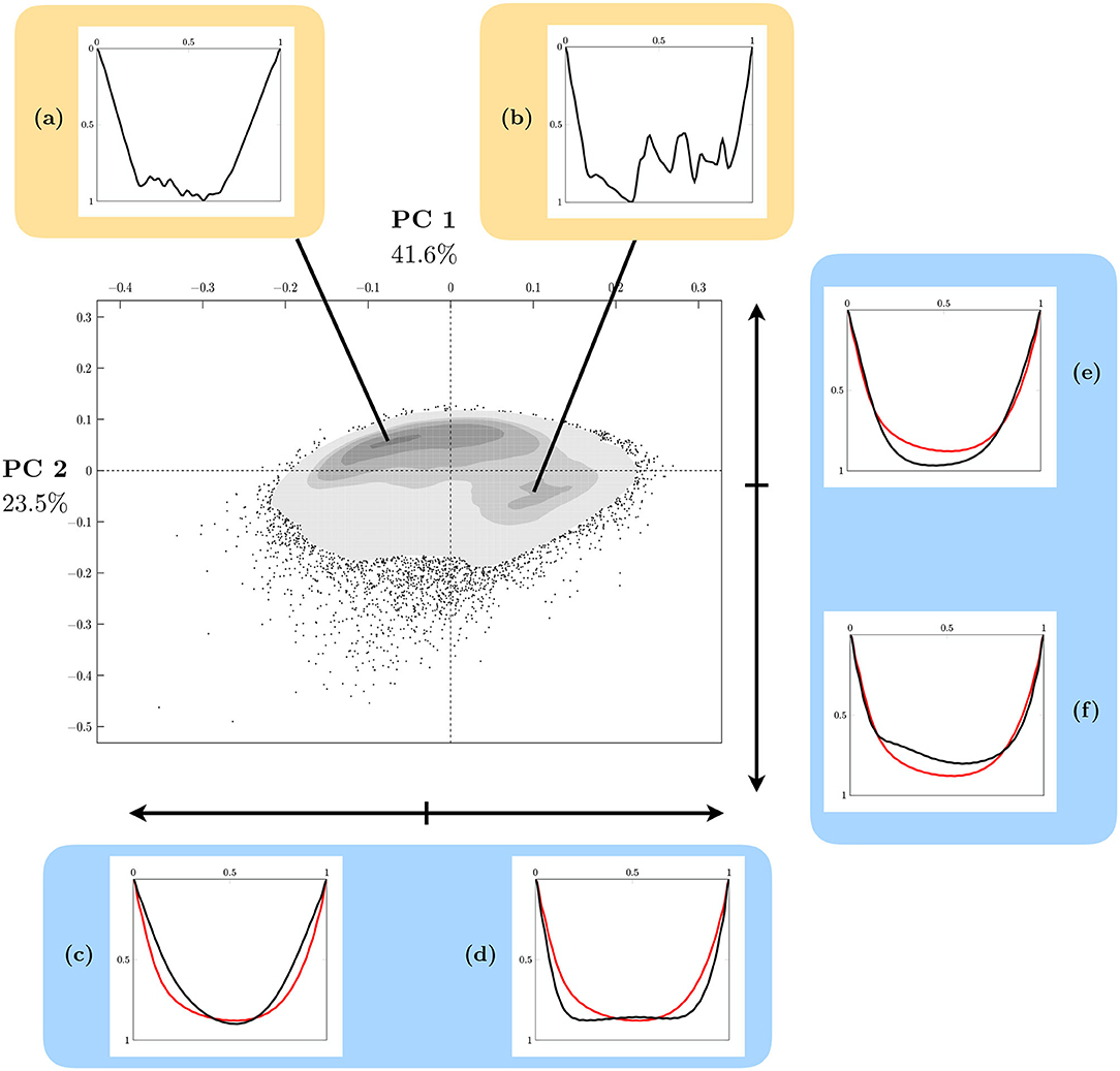
Figure 8. Kernel density display of the 2D FPCA map of dives of southern elephant seals. It accounts for 65.1% of the entire shape variability. The successive gray surfaces increasingly darker correspond to those containing, respectively 2.5, 25, 50, 75, and 97.5% of the data centered around local density maximums. Black points are those that escape the 97.5% area. At the top, normalized sample dives corresponding to the closest curves to the local maximums of density (a,b). At the bottom, representation of the influence of the first factorial axis (41.6% of explained variance) on the shape of the normalized curves (c,d). On the right, the influence of the second one (23.5% variance explained) (e,f). Red curves correspond to the mean curve. Black curves represent the deformation generated by the corresponding factor.

Pattern Identification and Relationship With Prey Capture Events (PCE)

Taking advantage of the FPCA dimension reduction, the MBC algorithm is realized in the space of the Q = 5 first principal components accounting for 87.3% of the entire variability. Clustering in the space of principal components will make the composition of the clusters more robust if changes occur in sample composition. We identified a number of 8 clusters whose mean and quantile curves are represented in Figure 9 (outliers are excluded).

FIGURE 9

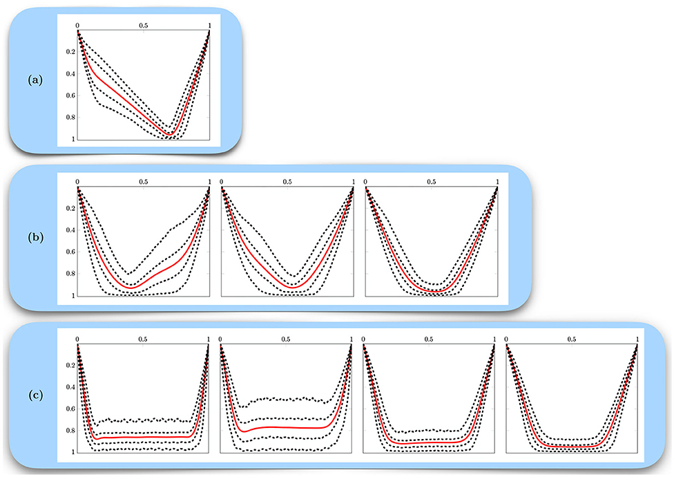
Figure 9. The different clusters of dives. The 2.5, 25, 75, and 97.5% quantile curves are in black dotted lines. Cluster mean curves are in solid red lines. The three categories are (a) drift, (b) exploratory, and (c) active according to the literature. Clusters in category (c) are sorted according to decreasing mean time spent at the bottom.

According to Dragon et al. (2012), dive shapes can be categorized as drift, exploratory and active dives [respectively (A), (B), and (C)]. Note that drift dives are non-symmetric dives with low variability in opposition to the other clusters. Additionally, exploratory and active dives are distinguished by their shape: V-shape for the first and square-shape for the second. However, differences occur within the same category. These differences are represented by a slight modification of the global shape due to time spent at the bottom, or variability expressed by discrepancies of the quantile curves. Active dives are sorted according to the duration of the bottom time. The behavioral meanings of the dive clusters and their differences will be discussed in detail in the Discussion section. The dive clusters will, now, be labeled according to their position in Figure 9 (i.e., drift, exploratory 1, active 3).

Identified patterns of dive shapes can be connected to foraging behaviors through the number of prey capture events (PCE) during dives. As a reminder, PCE are estimated according to the analysis of TDR-accelerometer data (Viviant et al., 2010).

The distribution of prey capture events (PCE) varies clearly according to the 8 dive shapes categories, as illustrated in Figure 10. As expected, drift dives are characterized by the fewest number of PCE (median close to 0). In contrast, foraging dives have the highest PCE values with a clear ranking in the median number of PCE according to the four foraging-dives categories evidenced by the functional analysis approach. Differences in foraging efficiency during active dives match with the proportion of bottom time and sinuosity during the bottom phase. Exploratory dives categories exhibit intermediate PCE values.

FIGURE 10

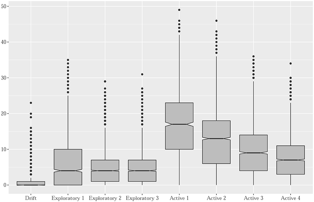
Figure 10. Boxplots of the number of estimated prey capture events per cluster. Labels identify the three major categories of diving behaviors.

Robustness of the Approach

We compare in this section, the efficiency of both classical PCA with numerical descriptors as variables and FPCA on dive curves through simulations of increasing downsampled datasets. Krzanowski distance is calculated between the reference FPCA (resp. PCA) and other FPCAs (resp. PCAs) on downsampled data (Figure 11).

FIGURE 11

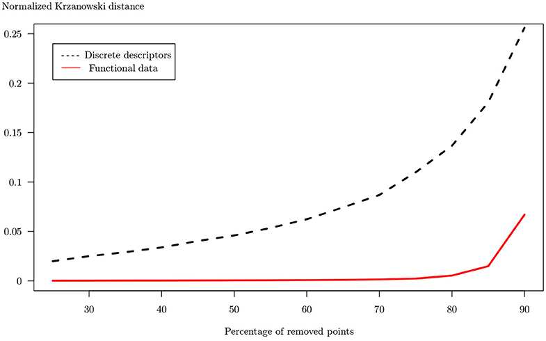
Figure 11. Krzanowski distance calculated between reference PCA of raw dives and PCAs of downsampled dives in functional case (red line) and using classic descriptors (black dotted line). Each raw dive has been downsampled by removing a percentage of points ranging from 20 to 90% by 5%. Both distances have been normalized for the ease of comparison.

In the functional case, the distance remains close to 0 up to 80% degradation. In the case where classical descriptors are used, the distance increases from the beginning to obtain a maximum at 90% degradation, which is much higher than in the functional case (0.26 compared with 0.07).

Discussion

In this study, we propose some statistical methods to cluster dives into categories which are ecologically appropriate and consistent with previous dives classification methods by distinguishing resting, exploring, and foraging dives. The characterization of dive shape combined with PCE allows the identification of particular foraging behaviors conditional to prey density. It therefore provides information on the spatial and temporal distribution of resources. The originality of this work is to consider the functional nature of the data: dives are curves, and the statistical methods include this property. It is then possible to study a sample of dive curves using the shape of the dives. Classification with MBC allows the identification of more diving behavior subcategories within each main diving categories proposed in the literature. These dive categories are ecologically relevant in terms of variation in the number of prey catch events. Even if many factors (e.g., environmental or physiological variables) can drive foraging behaviors, each dive category matches to a different level of prey catch levels. Furthermore, the proposed methods are more robust to downsampled data than previous classification methods based on numerical descriptors.

In this study, the physical dimensions of dives (time and depth) are deliberately excluded by a normalization step when focusing on the shape analysis of dives. Putting dives back to their real dimensions is a mandatory task to make the connection between dive shape and real physical variables (related to depth and time mostly). In other words, the study of dive shape does not prevent the computation of classical numerical descriptors. However, dive shape analysis provides some additional information.

Dives are characterized by three major factors (section 2.3Shape Characterization and Comparison). The first one is associated with variations in the proportion of bottom time (U or V shape), irrespective of the absolute bottom time, a usual descriptor specific to each dive. The second one is associated with variations in vertical movements during the bottom time, as defined as sinuosity, a numerical descriptor as in Bailleul et al. (2008). The third one is attached to variations in asymmetry in shape, the equivalent of which is not available as a numerical descriptor. This asymmetry is found in many diving species: pinnipeds, sea-birds, and seals (Schreer et al., 2001). The role and the origin of this asymmetry are manifold. In some cases, asymmetry is an indicator of body conditions (i.e., buoyancy). Vertical ascent speed tends to be more constrained than descent speed, likely in response to ecophysiological constraints to reduce the risk of decompression accident (see Richard et al., 2014). The proposed methods are, therefore, able to identify the importance of this asymmetry factor in an automated way.

Looking now at the clustering, eight dive clusters have been labeled as drift, exploratory, and active (Figure 9). These groups own characteristic shapes, which are a mixture of the three previous factors identified with FPCA accounting for about 80% of the variability between curves. Among then, the first category of dives corresponds to drift dives or resting/food processing dives (Crocker et al., 1997; Mitani et al., 2010). Exploratory dives are traveling and/or observation dives. Active dives are associated with foraging because individuals optimize the duration of bottom time to increase overall foraging success (Hindell et al., 1991; Fedak et al., 2001). However, the analysis of dive shapes suggests that it is more a question of optimizing the proportion of bottom time (according to the duration of the dive) more than the absolute bottom time. It could provide support for a non-linear relationship between search time and prey acquisition (Thums et al., 2012). The vertical depth variability (i.e., sinuosity) during the bottom phase of active dive clusters expresses movements related to prey captures. These two criteria have a real and well-known behavioral meaning. A proportion of 72–76% of the feeding events takes place during the bottom phase of the dive (Guinet et al., 2014; Jouma'a et al., 2016). Le Bras et al. (2016) also shows that the higher the sinuosity of the bottom phase of the dive over a narrower depth range (i.e., a limited depth range), the higher the number of PCE. The different classes of foraging dives are mainly driven by the vertical accessibility of the prey (close to the surface to deep) and their distribution within the water column (aggregated or dispersed over narrow or large layers). Most of the dive range bottom duration time of southern elephant seals tends to increase with prey encounter (Jouma'a et al., 2016). Therefore, the variation in southern elephant seal behavior at the bottom of their foraging dive constitutes, as we should expect, a response to the variation of the prey distribution with an increase in PCE during foraging dives. It is reflected by the variation of the number of PCE for each dive cluster. Foraging dives, that have the longest bottom time, have the highest number of PCE (boxplots in Figure 10). The differences in the variability, series of changes in depth, underline the link between foraging behavior and spatial distribution of prey patches. Active 1 class has less variability but more PCE. It can be assumed that more dense, less dispersed patches allow individuals a higher number of captures.

Characteristic shapes in clusters can be compared to numerical descriptors computed from raw data (Table 1). The relative proportion of each group varies, with active dives being the most represented and drift dives the least. Active 1 and 2 are the shallowest. Active 3 and 4 are deepest. There are, therefore, two groups of active dive clusters: shallow active (1 and 2) with more PCE, and deep active (3 and 4). The longer the duration of the bottom time, the shallower the dives, and the higher the number of PCE. Active dives maximize foraging time by minimizing descent and ascent time.

TABLE 1

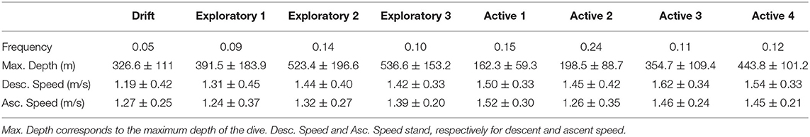
Table 1. Characteristics of dive clusters. All differences between median of these groups are statistically significant (p < 0.001, Kruskal Wallis test).

Except exploratory 1 cluster, exploratory dives are the deepest, and they have the lowest duration of bottom time. Exploratory 1 dives have a skewed left shape, and the other exploratory dives have a V-shape. These are observation and/or traveling dives. Drift dives have a reasonable maximum depth with low descent and ascent speed. Individuals make little effort during these dives. In addition, the number of PCE is close to 0 (Figure 10). It is in line with the hypothesis that these dives are food processing and/or resting dives. Even if they are scarce, these drift dives are very well and identified in an automated way using the FDA approach.

During a foraging migration of an animal, it happens that the retrieved data are damaged due to sensor problems. Furthermore, when tags are not recovered, only a few depth points per dives are transmitted by satellite (Boehme et al., 2009). Classically, the transmitted depth points are selected through a broken-stick approach (Heerah et al., 2014). The FDA approach can be useful to optimize the transmitted amount of data. For instance, it is possible to transmit fewer basis coefficients to reconstruct the entire profile easily. It is also possible to optimize the position of spline knots to get an accurate fitted profile with few coefficients. The FDA approach is also suitable for processing and comparing dive data with different sampling frequencies. This particular point has been illustrated through the analysis of simulated data sets. Our results show that the functional data analysis is more resilient to corrupted data compare to classification methods relying on discrete dive descriptors. Furthermore, the FDA computation time is significantly shorter than the computation time with the broken-stick algorithm. The computation time for the FDA approximation of N = 87, 691 entire curves was 357s against 4, 404s for the broken-stick algorithm on a 2.7GHz processor. The broken-stick algorithm gives only 6 pairs of time-depth points, whereas the FDA approximation is pretty good, taking a basis expansion with six coefficients as previously shown in Figure 3. This information is relevant when aiming at reducing computation time and, therefore, energy consumption for onboard processing and real-time transmission of dive profiles.

Conclusions and Perspectives

This study demonstrates the potentiality of the FDA method for the characterization and the classification of time-depth dive profiles. Using the shape of dive profiles enables us to obtain, in a very visual way, results that are ecologically consistent and coherent with previous dive classification methods implemented on elephant seal diving data. Moreover, diving behaviors of Mirounga leonina are straightforwardly related to a small number of independent factors connected to shape variations in dives and to account for most of the entire variability in curve shape. The processed data set is large (N = 87, 691 dives), and FDA makes it possible to process large amounts of data automatically and quickly. Such an approach will be relevant to conduct analyses, such as inter-annual or longer-term variations in the diving behavior of the elephant seal. Besides, the proposed methods allow the efficient discrimination of drift dives used to monitor the change of buoyancy, and therefore, body condition of the seal during their migration. Studying the ratio between buoyancy (obtained thanks to the asymmetry of dives with principal component scores) and the number of active dives would highlight the foraging efficiency of individuals in geographical areas of interest. The use of FDA allows the correct processing of downsampled data. It is possible to process low frequency transmitted data from unrecovered tags and to compare them with high-frequency data. It is a real advantage if one considers the possibility to compare high-frequency current data to less accurate historical recorded data. Finally, the new results of this study raise further questions on the origin of the diving behaviors and on the forces that shape them. The next promising step is to integrate environmental covariates (temperature, salinity, and chlorophyll) that can also be considered as profiles better to understand links between dive curve shapes and behaviors.

Data Availability Statement

The dataset analyzed for this study can be found in the MEOP-CTD database (Treasure et al., 2017), http://www.meop.net/.

Ethics Statement

The animal study was reviewed and approved by the TAAF Ethics Committee (Comite Environnement et Préfet des Terres Australes et Antarctiques Francaises).

Author Contributions

MG conceived the idea and wrote the manuscript. MG, CM, and DN analyzed the data and prepared the figures. CM, DN, CG, and BP corrected the manuscript and helped for important results interpretations. MG, CG, and BP carried out the fieldwork. CG and BP provided additional data. All authors contributed to the article and approved the submitted version.

Funding

The Ph.D. scholarship of MG was funded by the French Ministry for Education and Research.

Conflict of Interest

The authors declare that the research was conducted in the absence of any commercial or financial relationships that could be construed as a potential conflict of interest.

Acknowledgments

The authors acknowledge two reviewers for their very constructive comments on earlier versions of the manuscript. We thank all people involved in the fieldwork, Hazel Pittwood and Benjamin Girardot for correction of the English.

Supplementary Material

The Supplementary Material for this article can be found online at: https://www.frontiersin.org/articles/10.3389/fmars.2020.00595/full#supplementary-material

References

Bailleul, F., Pinaud, D., Hindell, M., Charrassin, J. B., and Guinet, C. (2008). Assessment of scale-dependent foraging behaviour in southern elephant seals incorporating the vertical dimension: a development of the first passage time method. J. Anim. Ecol. 77, 948–957. doi: 10.1111/j.1365-2656.2008.01407.x

PubMed Abstract | CrossRef Full Text | Google Scholar

Biernacki, C., Celeux, G., and Govaert, G. (2000). Assessing a mixture model for clustering with the integrated completed likelihood. IEEE Trans. Pattern Anal. Mach. Intell. 22, 719–725. doi: 10.1109/34.865189

CrossRef Full Text | Google Scholar

Block, B. A., Jonsen, I. D., Jorgensen, S. J., Winship, A. J., Shaffer, S. A., Bograd, S. J., et al. (2011). Tracking apex marine predator movements in a dynamic ocean. Nature 475, 86–90. doi: 10.1038/nature10082

PubMed Abstract | CrossRef Full Text | Google Scholar

Boehme, L., Lovell, P., Biuw, M., Roquet, F., Nicholson, J., Thorpe, S. E., et al. (2009). Technical note: animal-borne ctd-satellite relay data loggers for real-time oceanographic data collection. Ocean Sci. 5, 685–695. doi: 10.5194/os-5-685-2009

CrossRef Full Text | Google Scholar

Campagna, C., Boeuf, B. L., Blackwell, S., Crocker, D., and Quintana, F. (1995). Diving behaviour and foraging location of female southern elephant seals from patagonia. J. Zool. 236, 55–71. doi: 10.1111/j.1469-7998.1995.tb01784.x

CrossRef Full Text | Google Scholar

Crocker, D. E., LeBoeuf, B. J., and Costa, D. P. (1997). Drift diving in female northern elephant seals: implications for food processing. Can J Zool. 75, 27–39. doi: 10.1139/z97-004

CrossRef Full Text | Google Scholar

Dragon, A., Bar-Hen, A., Monestiez, P., and Guinet, C. (2012). Horizontal and vertical movements as predictors of foraging success in a marine predator. Mar. Ecol. Prog. Ser. 447, 243–257. doi: 10.3354/meps09498

CrossRef Full Text | Google Scholar

Dryden, I. L., and Mardia, K. V. (2016). Statistical Shape Analysis: With Applications in R, Vol. 995. Chichester: John Wiley & Sons.

Google Scholar

Evans, K., Lea, M.-A., and Patterson, T. (2013). Recent advances in bio-logging science: technologies and methods for understanding animal behaviour and physiology and their environments. Deep Sea Res. II Top. Stud. Oceanogr. 88–89, 1–6. doi: 10.1016/j.dsr2.2012.10.005

CrossRef Full Text | Google Scholar

Fedak, M. a, Lovell, P., and Grant, S. M. (2001). Two approaches to compressing and interpreting time-depth information as collected by time-depth recorders and satellite-linked data recorders. Mar. Mammal Sci. 17, 94–110. doi: 10.1111/j.1748-7692.2001.tb00982.x

CrossRef Full Text | Google Scholar

Fedak, M., Lovell, P., McConnell, B., and Hunter, C. (2002). Overcoming the constraints of long range radio telemetry from animals: getting more useful data from smaller packages. Integr. Compar. Biol. 42, 3–10. doi: 10.1093/icb/42.1.3

PubMed Abstract | CrossRef Full Text | Google Scholar

Fraley, C., and Raftery, A. (2002). Model-based clustering, discriminant analysis, and density estimation. J. Am. Stat. Assoc. 97, 611–631. doi: 10.1198/016214502760047131

CrossRef Full Text | Google Scholar

Guinet, C., Vacquié-Garcia, J., Picard, B., Bessigneul, G., Lebras, Y., Dragon, A. C., et al. (2014). Southern elephant seal foraging success in relation to temperature and light conditions: insight into prey distribution. Mar. Ecol. Prog. Ser. 499, 285–301. doi: 10.3354/meps10660

CrossRef Full Text | Google Scholar

Harcourt, R., Martins Sequeira, A. M., Zhang, X., Rouquet, F., Komatsu, K., Heupel, M., et al. (2019). Animal-borne telemetry: an integral component of the ocean observing toolkit. Front. Mar. Sci. 6:326. doi: 10.3389/fmars.2019.00326

CrossRef Full Text | Google Scholar

Heerah, K., Hindell, M., Guinet, C., and Charrassin, J.-B. (2014). A new method to quantify within dive foraging behaviour in marine predators. PLoS ONE 9:e0099329. doi: 10.1371/journal.pone.0099329

PubMed Abstract | CrossRef Full Text | Google Scholar

Hindell, M. A., McMahon, C. R., Bester, M. N., Boehme, L., Costa, D., Fedak, M. A., et al. (2016). Circumpolar habitat use in the southern elephant seal: implications for foraging success and population trajectories. Ecosphere 7:e01213. doi: 10.1002/ecs2.1213

CrossRef Full Text | Google Scholar

Hindell, M. A., Slip, D. J., and Burton, H. R. (1991). The diving behaviour of adult male and female southern elephant seals, Mirounga leonina (Pinnipedia: Phocidae). Aust. J. Zool. 39, 499–508. doi: 10.1071/ZO9910595

CrossRef Full Text | Google Scholar

Jonsen, I. D., Myers, R. A., and James, M. C. (2007). Identifying leatherback turtle foraging behaviour from satellite telemetry using a switching state-space model. Mar. Ecol. Prog. Ser. 337, 255–264. doi: 10.3354/meps337255

CrossRef Full Text | Google Scholar

Jouma'a, J., Le Bras, Y., Richard, G., Vacquié-Garcia, J., Picard, B., El Ksabi, N., et al. (2016). Adjustment of diving behaviour with prey encounters and body condition in a deep diving predator: the southern elephant seal. Funct. Ecol. 30, 636–648. doi: 10.1111/1365-2435.12514

CrossRef Full Text | Google Scholar

Kooyman, G. L. (2012). Diverse Divers: Physiology and Behavior, Vol. 23. Berlin: Springer Science & Business Media.

Google Scholar

Krzanowski, W. (2000). Principles of Multivariate Analysis, Vol. 23. Oxford: OUP Oxford.

Google Scholar

Le Boeuf, B., Crocker, D., Blackwell, S., Morris, P., and Thorson, P. (1993). Sex differences in diving and foraging behaviour of northern elephant seals. Symp. Zool. Soc. Lond. 66, 149–178.

Google Scholar

Le Bras, Y., Jouma,'A, J, Picard, B., and Guinet, C. (2016). How elephant seals (mirounga leonina) adjust their fine scale horizontal movement and diving behaviour in relation to prey encounter rate. PLoS ONE 11:e0167226. doi: 10.1371/journal.pone.0167226

PubMed Abstract | CrossRef Full Text | Google Scholar

McMahon, C. R., Burton, H., Slip, D., McLean, S., and Bester, M. (2000). Field immobilisation of southern elephant seals with intravenous tiletamine and zolazepam. Vet. Rec. 146, 251–254. doi: 10.1136/vr.146.9.251

PubMed Abstract | CrossRef Full Text | Google Scholar

Melnykov, V., and Maitra, R. (2010). Finite mixture models and model-based clustering. Stat. Surv. 4, 80–116. doi: 10.1214/09-SS053

CrossRef Full Text | Google Scholar

Mitani, Y., Andrews, R. D., Sato, K., Kato, A., Naito, Y., and Costa, D. P. (2010). Three-dimensional resting behaviour of northern elephant seals: drifting like a falling leaf. Biol. Lett. 6, 163–166. doi: 10.1098/rsbl.2009.0719

PubMed Abstract | CrossRef Full Text | Google Scholar

Ngô, M. C., Heide-Jørgensen, M. P., and Ditlevsen, S. (2019). Understanding narwhal diving behaviour using hidden markov models with dependent state distributions and long range dependence. PLoS Comput. Biol. 15, 1–21. doi: 10.1371/journal.pcbi.1006425

PubMed Abstract | CrossRef Full Text | Google Scholar

Nowacek, D. P., Christiansen, F., Bejder, L., Goldbogen, J. A., and Friedlaender, A. S. (2016). Studying cetacean behaviour: new technological approaches and conservation applications. Anim. Behav. 120, 235–244. doi: 10.1016/j.anbehav.2016.07.019

CrossRef Full Text | Google Scholar

Ramsay, J., and Silverman, B. (2005). Functional Data Analysis, 2nd Edn. New York, NY: Springer.

Google Scholar

Richard, G., Vacquié-Garcia, J., Joumaá, J., Picard, B., Génin, A., Arnould, J. P. Y., et al. (2014). Variation in body condition during the post-moult foraging trip of southern elephant seals and its consequences on diving behaviour. J. Exp. Biol. 217, 2609–2619. doi: 10.1242/jeb.088542

PubMed Abstract | CrossRef Full Text | Google Scholar

Roquet, F., Williams, G., Hindell, M. A., Harcourt, R., McMahon, C., Guinet, C., et al. (2014). A southern indian ocean database of hydrographic profiles obtained with instrumented elephant seals. Sci. Data 1:140028. doi: 10.1038/sdata.2014.28

PubMed Abstract | CrossRef Full Text | Google Scholar

Runge, C. A., Martin, T. G., Possingham, H. P., Willis, S. G., and Fuller, R. A. (2014). Conserving mobile species. Front. Ecol. Environ. 12, 395–402. doi: 10.1890/130237

CrossRef Full Text | Google Scholar

Scheffer, A., Bost, C.-A., and Trathan, P. N. (2012). Frontal zones, temperature gradient and depth characterize the foraging habitat of king penguins at south georgia. Mar. Ecol. Prog. Ser. 465, 281–297. doi: 10.3354/meps09884

CrossRef Full Text | Google Scholar

Schreer, J. F., Kovacs, K. M., and O'Hara Hines, R. J. (2001). Comparative diving patterns of pinnipeds and seabirds. Ecol. Monogr. 71, 137–162. doi: 10.1890/0012-9615(2001)071[0137:CDPOPA]2.0.CO;2

CrossRef Full Text | Google Scholar

Stephens, D. W., and Krebs, J. R. (1986). Foraging Theory. Chichester: Princeton University Press.

Google Scholar

Thums, M., Bradshaw, C. J., and Hindell, M. A. (2008). A validated approach for supervised dive classification in diving vertebrates. J. Exp. Mar. Biol. Ecol. 363, 75–83. doi: 10.1016/j.jembe.2008.06.024

CrossRef Full Text | Google Scholar

Thums, M., Bradshaw, C. J., Sumner, M. D., Horsburgh, J. M., and Hindell, M. A. (2012). Depletion of deep marine food patches forces divers to give up early. J. Anim. Ecol. 82, 72–83. doi: 10.1111/j.1365-2656.2012.02021.x

PubMed Abstract | CrossRef Full Text | Google Scholar

Treasure, A., Roquet, F., Ansorge, I., Bester, M., Boehme, L., Bornemann, H., et al. (2017). Marine mammals exploring the oceans pole to pole: a review of the MEOP consortium. Oceanography 30, 132–138. doi: 10.5670/oceanog.2017.234

CrossRef Full Text | Google Scholar

Tremblay, Y., and Cherel, Y. (2000). Benthic and pelagic dives: a new foraging behaviour in rockhopper penguins. Mar. Ecol. Prog. Ser. 204, 257–267. doi: 10.3354/meps204257

CrossRef Full Text | Google Scholar

Viviant, M., Trites, A. W., Rosen, D. A., Monestiez, P., and Guinet, C. (2010). Prey capture attempts can be detected in steller sea lions and other marine predators using accelerometers. Polar Biol. 33, 713–719. doi: 10.1007/s00300-009-0750-y

CrossRef Full Text | Google Scholar

Watwood, S. L., Miller, P. J. O., Johnson, M., Madsen, P. T., and Tyack, P. L. (2006). Deep-diving foraging behaviour of sperm whales (Physeter macrocephalus). J. Anim. Ecol. 75, 814–825. doi: 10.1111/j.1365-2656.2006.01101.x

PubMed Abstract | CrossRef Full Text | Google Scholar