Multi-Layered High Permeability Conduits Connecting Onshore and Offshore Coastal Aquifers

Introduction

Coastal groundwater systems represent the zone where terrestrial groundwater meets intruded higher-density seawater, which in turn drives groundwater flow processes beneath the coastline (Jiao and Post, 2019). They are important pathways for material transport across the coastal transition zone where active cycling of macronutrients and trace metals occurs (Moore, 2010). Groundwater seepage to coastal waters via subterranean estuaries can trigger toxic algae blooms and can have adverse impacts on the ecosystems and the economy of many coastal communities (Moore, 1999). Generally, seawater can intrude inland in response to excessive water withdrawals, or upconing (Barlow, 2003), whereas groundwater from terrestrial coastal aquifers may discharge through the seafloor as submarine groundwater discharge (SGD). SGD is defined as any flow of water out across the seafloor regardless of composition, origin, or the mechanisms driving the flow (Burnett et al., 2006). In all coastal zones, SGD occurs wherever an onshore aquifer with a positive head relative to sea level is hydraulically connected to the ocean (Johannes, 1980; Moore, 1996). SGD is intermittent, occurs in various geologic settings (e.g., carbonate and siliciclastic), and sometimes involves multiple aquifers (Burnett et al., 2006; Bratton, 2010).

A less commonly studied characteristic of coastal aquifers is the occurrence of, and possible connection to, vast meteoric groundwater reserves (Post et al., 2013), or termed herein as offshore freshened groundwater (OFG) systems. These systems are becoming the focus of rigorous study because of their potential to mitigate water stress in coastal areas including, for example; Cape Town, Sao Paolo, Malta, Chennai, Singapore, Beijing, and Jakarta (Ferguson and Gleeson, 2012; Michael et al., 2017; Moosdorf and Oehler, 2017; Post et al., 2018; Berndt and Micallef, 2019). The connection between onshore and offshore coastal aquifers has important implications for the potential exploitation and management of offshore groundwater reserves, but remains poorly understood partly because of (1) barriers across disciplines that inhibit interdisciplinary research (Talley et al., 2003), (2) difficulty with integrating geophysical and geochemical methods to characterize groundwater systems across the coastal transition zone (Post, 2005), and (3) the lack of appropriate technologies to map and quantify zones of freshwater flow offshore (Post, 2005; Evans, 2007), particularly in the nearshore environment, or so-called ‘White Ribbon’ (Leon et al., 2013). Presently there is no simple way to gauge fluxes of meteoric groundwater to the sea. However, new strides are being made by employing geophysical methods, notably marine electromagnetics (Gustafson et al., 2019; Micallef et al., 2020), as a means to guide geochemical sampling, and ultimately to inform hydrogeological modeling efforts to quantify the evolution of coastal groundwater systems in response to changing sea level and possible extraction.

Over geologic timescales, terrestrial aquifers can migrate landwards or seawards in response to rising and falling sea levels, respectively. During the Last Glacial Maximum, modern continental shelf areas were subaerially exposed and subjected to infiltration of atmospheric precipitation (meteoric water) and in high latitudes where ice sheets form drained by glacial meltwater (Person et al., 2007; Cohen et al., 2010). During low sea levels, shore-normal flow, which results from an increase in the hydraulic head onshore and steep onshore gradients, played a key role in driving freshwater offshore and extending OFG systems further out into the continental shelf (Johnston, 1983). It has been shown that OFG systems adjust slowly to rising sea levels over long time scales (Person et al., 2003) and, as a result, remnants of meteoric groundwater occur offshore in many places worldwide. The global inventory of OFG systems as described by Post et al. (2013) has been estimated primarily through a combination of observations from boreholes, both onshore and offshore, or by modeling studies to total around 5 × 10⁵ km³. The majority of these systems have either a direct or inferred terrestrial connection; however, a lack of observational data, especially across the coastal transition zone, precludes a comprehensive understanding of offshore connectivity to aquifers onshore (Figure 1). Pore-water profiles in low-permeability layers investigated on continental shelves around the world (e.g., North Sea, Peru, and New Zealand) show a consistent vertical salinity decrease (Post et al., 2013) indicating past meteoric circulation. An important distinction yet to be clarified is whether these connections are active or inactive. Recent marine electromagnetic imaging surveys provide strong evidence for onshore connections to the US Atlantic Continental Shelf (Gustafson et al., 2019) and offshore New Zealand (Micallef et al., 2020). However, it should be noted that electromagnetic techniques provide only static snapshots of subsurface resistivity structure and hence cannot constrain flow dynamics.

FIGURE 1

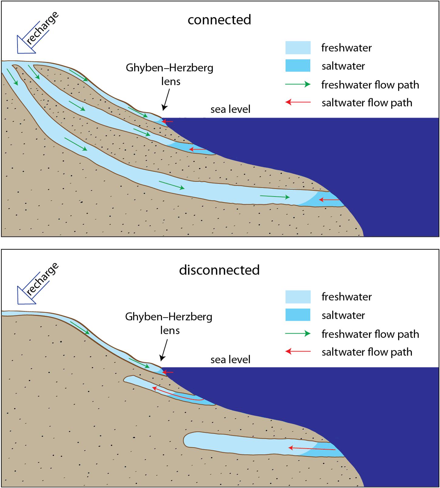
Figure 1. Cartoon depicting the differences between offshore freshened groundwater (connected) and paleo-groundwater (disconnected) systems. Modern day “active” aquifers are recharged by precipitation (green arrows). Fossil aquifers are no longer fed by meteoric water, however, both systems are subject to saltwater intrusion becoming saline over time (red arrows).

Electromagnetic (EM) methods are suitable for delineating occurrences of groundwater in coastal environments. EM methods measure the bulk electrical conductivity (σ), or resistivity (ρ) (note: σ = 1/ρ) structure of the subsurface, which is mainly governed by the salinity of pore fluids, the porosity of sediments, and the connectivity of the pore space (Evans and Lizarralde, 2011). Archie’s Law (Archie, 1942) provides a means to estimate pore fluid salinity, assuming porosity variations are known, or can be estimated. Freshwater (∼ 10–500 mS/m) is orders of magnitude less conductive than seawater (∼ 1,000–5,000 mS/m) (Palacky, 1988); therefore, mapping σ contrasts can help to characterize the presence of freshwater within the sediment pore space. EM measurements are routinely used to map terrestrial aquifers and guide hydrological sampling (e.g., Burnett et al., 2006; Swarzenski and Izbicki, 2009) and have been employed in a variety of coastal settings (e.g., Delefortrie et al., 2014; Weymer et al., 2016). These and other papers demonstrate their utility for detecting the variable hydrogeology beneath modern coastlines.

One example of a well-studied terrestrial aquifer system is the Canterbury Plains, South Island, New Zealand. A considerable amount of monitoring well and borehole information is available, making the area an ideal calibration site to conduct geophysical surveys. This study presents findings from geophysical surveys, using three complementary near-surface EM methods, to investigate potential groundwater pathways within braided alluvial deposits beneath a mixed sand-gravel (MSG) beach along the Ashburton coast, South Island, New Zealand. We integrate acquired ground penetrating radar (GPR), electromagnetic induction (EMI), and transient electromagnetic (TEM) data to test a hypothesis that high permeability gravel zones beneath the modern coastline act as conduits for groundwater flow offshore. Our study complements a large-scale geophysical survey conducted offshore along the Canterbury Bight to map OFG systems, for which a meteoric origin and present-day connection to onshore aquifers is inferred. Our results provide evidence that this newly discovered OFG system (Micallef et al., 2020) has been recharged in the past via these conduits and that the connection implies recharge by modern terrestrial aquifers underlying the Canterbury Plains.

Study Area

Our study site is situated within the greater Canterbury Plains and located along the eastern coastline of the South Island of New Zealand (Figure 2), approximately 8 km ENE from the Ashburton River mouth. Covering ∼ 8,000 km², the Canterbury Plains host an exceptional and well-utilized groundwater system (see Leckie, 2003). The plain consists of ∼ 600-m-thick broad fluvial megafan and glaciofluvial sheets that were emplaced by braided rivers draining from the Southern Alps during the Pleistocene and Holocene (Schumm and Phillips, 1986; Leckie, 2003). At the outcrop scale, sediments are mainly heterogeneous glaciofluvial gravels (95%) consisting of isolated sand bodies (on the order of meters thick and tens of meters wide) with minimal clay content (<0.3%) (Ashworth et al., 1999; Moreton et al., 2002).

FIGURE 2

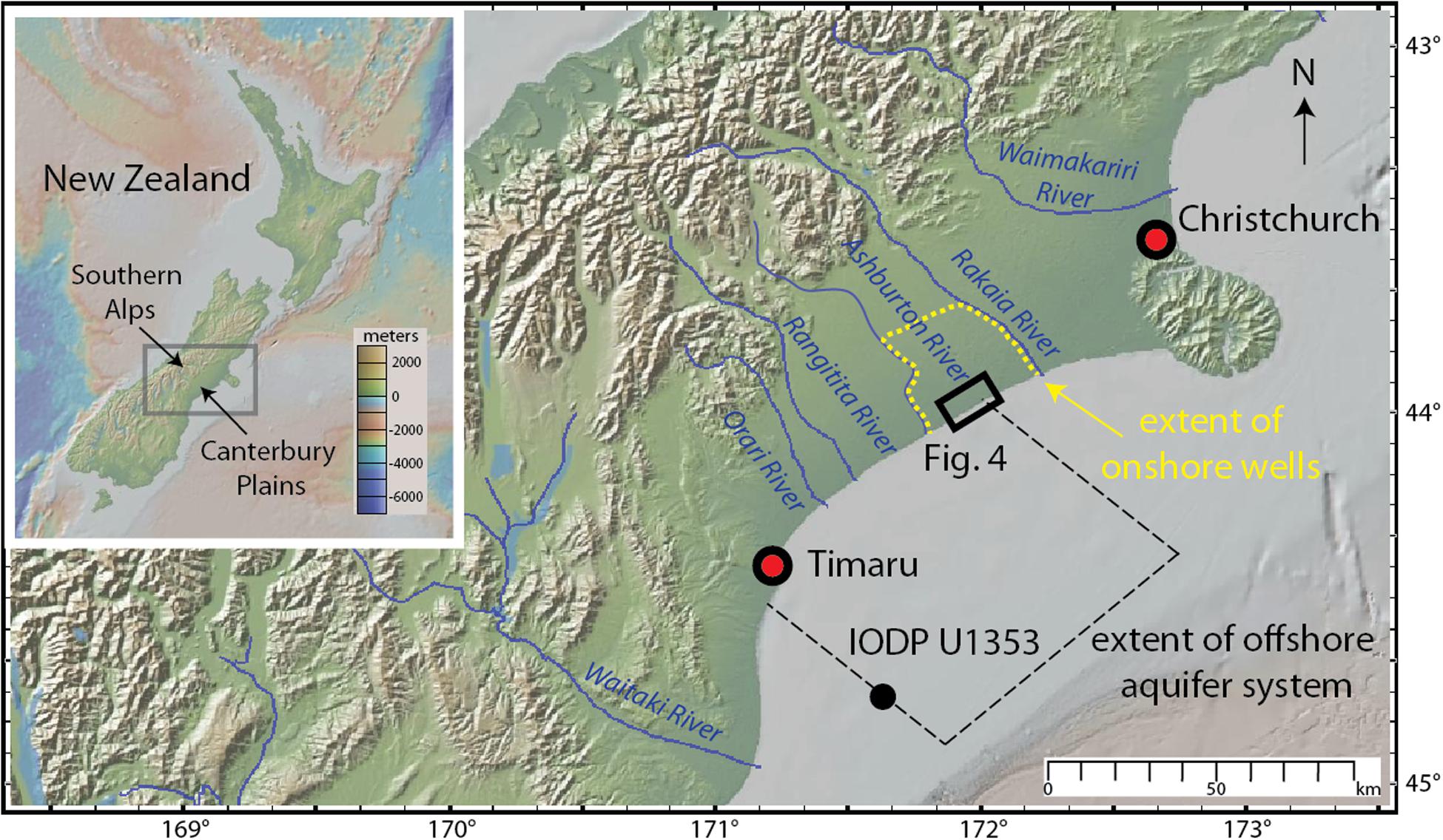
Figure 2. Map of New Zealand, and location of the study area in the Canterbury Plains region of the South Island, New Zealand. The approximate extent of the OFG system is outlined by the black dotted lines and the location of IODP borehole U1353 is shown as a reference. The region of the onshore monitoring wells from Davey (2004) is highlighted by the yellow dotted line. The location of the zoomed in area for the digital elevation model (DEM) in Figure 4 is outlined by the black box. Maps created using GeoMapApp (Ryan et al., 2009).

Terrestrial aquifers in the region between the Ashburton and Rakaia Rivers are fed by large catchments extending to the Southern Alps and have been characterized though an extensive network of monitoring wells (Bal, 1996; Davey, 2004). Three main aquifers identified on the basis of screen distribution are hosted in the gravels down to at least 150 m depth, with unconnected sand and silt/clay layers forming aquitards (Davey, 2006). The aquifers were found to be generally from ∼ 0–50 m, 50–90 m, and >90 m depths, whereas two aquitards were identified at roughly 50 m and between 80 and 90 m depth in an area NE of the Ashburton River (Davey, 2004). The regional flow of groundwater in the Canterbury aquifers is from the foothills of the Southern Alps toward the coastline (Mandel, 1974).

The alluvial braidplain that hosts the gravel aquifers was studied in detail by Bal (1996) where five to six high permeability corridors (roughly 5–10 km wide), inferred to be infilled or buried valleys have been suggested to act as preferred groundwater flow paths that trend roughly perpendicular to the coastline. In a subsequent scale modeling study by Moreton et al. (2002) it was shown that at even smaller spatial scales (meters to tens of meters) secondary channel fill deposits preserved within the braided alluvial architecture have the coarsest grain size and highest permeability compared to all other facies (e.g., primary channel fills, splays, and fine-grained channels). This inference can be made both from the model experiments and field observations. The gravel lenses were shown to form as a result of coarse-grained sediments preferentially settling adjacent to or within a larger primary channel during peak flood discharge. Flows within the secondary channels were not large enough to allow channels to migrate between successive flood peaks. With this flow constriction, stalling of a sediment lobe formed a coarse-grained channel plug that preserved the cross-sectional geometry of the channel in the subsurface forming a high permeability conduit that may potentially discharge groundwater offshore. These channel deposits are visible along the coastal bluffs at the study site and are dissected by numerous composite channels or box canyons (Figure 3) hypothesized to have formed by groundwater sapping (Schumm and Phillips, 1986). The local geology at the study area consists of 15–20-m-high poorly sorted and uncemented matrix supported outwash gravels, which are capped by up to 1 m of post-glacial loess and modern soil (Berger et al., 1996). The cliff face is punctuated by isolated ∼ 0.5 m-thick sand lenses interbedded within clean gravels.

FIGURE 3

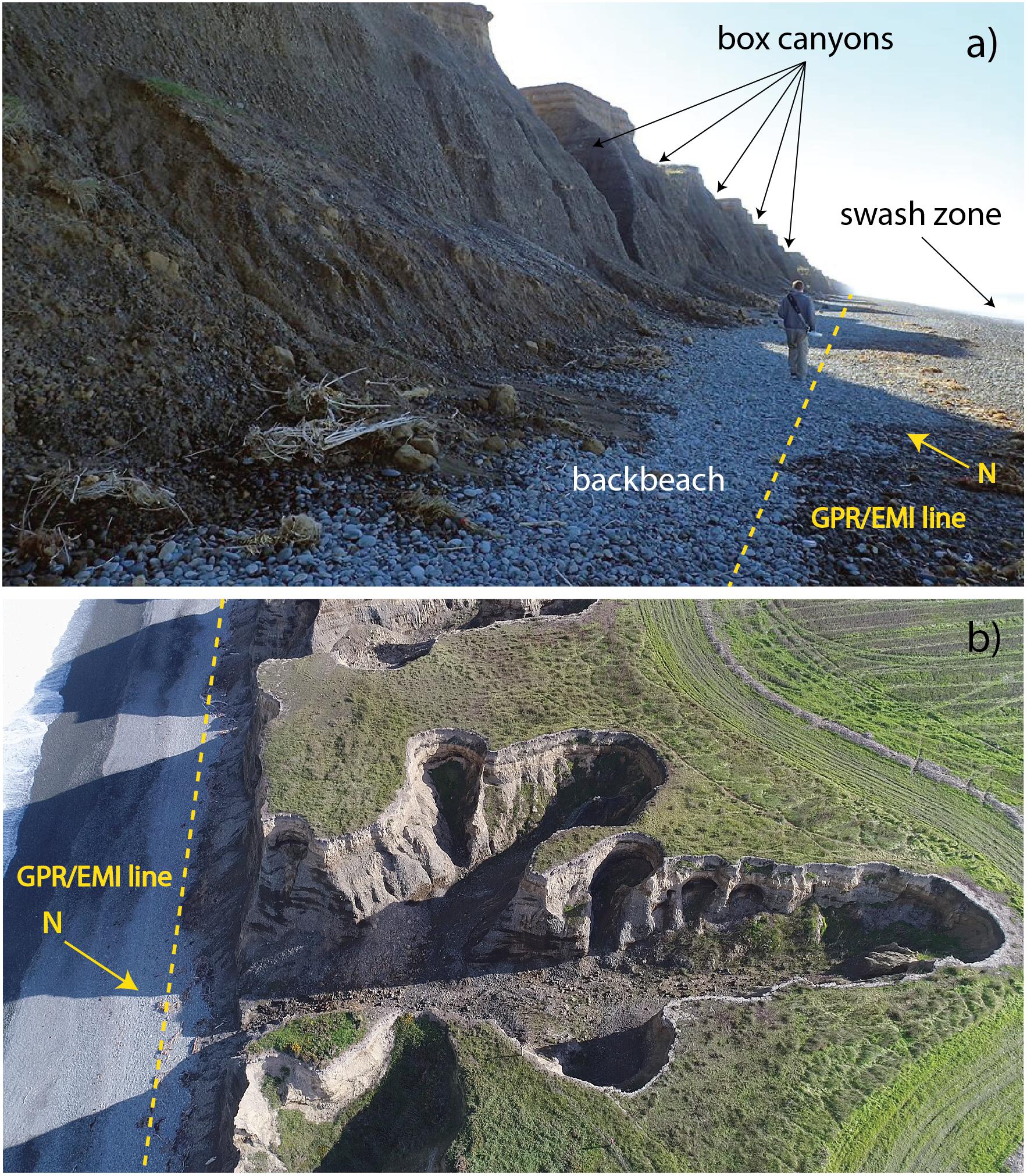
Figure 3. Image showing the location of the coincident alongshore GPR/EMI surveys and adjacent cliff and box canyon morphology (a). Aerial view (b) of a representative box canyon (view to the SE). Images taken between May 5–8, 2017.

The plain is transected by large, high-energy, gravel-bed rivers of mean annual flows 20–200 m³/s, with discharge up to 5,600 m³/s during flood events (Browne and Naish, 2003). The major rivers – Rangitata, Ashburton, Rakaia, and Waimakariri – incise the plains and flow toward a shoreline that is subject to the high-energy waves of the East Coast Swell (Davies, 1964), the Southland Current (Heath, 1981), and extreme storms. The latter contribute to sea cliff erosion rates ∼ 1 m/year (Schumm and Phillips, 1986). As a result, erosion of the coastline over the last ∼ 6.5 ka has produced a 70-km retrogradational coastline southwest of the Banks Peninsula providing a nearly continuous outcrop of the late Quaternary braided gravels (Moreton et al., 2002). According to Jennings and Shulmeister (2002), the Ashburton coastline exhibits morphodynamic characteristics of a mixed sand-gravel beach (MSG) classification. The beach morphology is reflective (Wright and Short, 1984) and the average beach width along the survey site is ∼ 30 m or less. The hydrodynamic regime is dominated by swash processes and plunging and/or collapsing waves that restrict alongshore sediment transport to mainly within the swash zone (Kirk, 1980). The tides are semi-diurnal with a mesotidal range, the spring range reaching 2.5 m (McLean, 1970).

Recent offshore electromagnetic geophysical surveying across the Canterbury Bight (Figure 2) identified a previously unknown OFG system (Micallef et al., 2020). This OFG system consists of one main, and two smaller, low salinity aquifers. The main aquifer extends up to a distance of 60 km perpendicularly from the coast, has a maximum thickness of at least 250 m, and its top reaches a maximum depth of 50 m bsf. It extends from offshore of Ashburton in the NE to offshore of Timaru in the SW, across an along-shelf distance of 72 km in water depths of up to 110 m. The smaller OFG bodies occur at shallower depths above the main OFG body. They are up to 15 km long, 50 m thick and have complex lenticular cross-sections. The minimum and maximum OFG volumes are estimated at 56 km³ and 213 km³, respectively, based on Archie’s Law calculations assuming constant porosities ranging from 20 to 40% representative of gravels to fine sands (see Micallef et al., 2020, p. 12).

Materials and Methods

This study utilizes near-surface geophysical methods to map high permeability groundwater conduits along the Canterbury coast. We chose three complementary non-invasive, near-surface electromagnetic (EM) techniques that are sensitive to spatial variations in bulk electrical conductivity σ and dielectric permittivity ε, both of which should be diagnostic of subsurface variations in hydrogeology. The instruments include: (1) GSSI Profiler EMP-400 EMI sensor; (2) Sensors & Software pulseEKKO GPR system; and (3) Geonics G-TEM time-domain electromagnetic (TDEM) system. Each instrument probes a different depth of investigation collectively ranging from ∼ 0 to 80 m for this particular coastal environment. The EMI system provides the shallowest depth of investigation ∼ 7 m, the GPR system is intermediate ∼ 9 m, while the G-TEM system probes deepest up to ∼ 80 m. A brief overview of each EM method is outlined below.

(1) Portable EMI rigid-boom sensors, or terrain conductivity meters, are a type of geophysical instrument that operates by monitoring the magnetic flux linkage between the ground and a transmitter (TX) coil through which a time-harmonic electric current of frequency ω is made to flow. The current in the TX coil generates a primary magnetic field B^p(r)e^iωt at the receiver (RX) coil, where r is the fixed TX-RX offset. Some of the primary field lines also flux through conductive bodies that are present in the subsurface, thereby generating an electromotive force. The latter causes eddy currents (somewhat analogous to hydrodynamic smoke rings) to flow in the subsurface. These produce a secondary magnetic field B^s(r)e^iωt, also monitored at the RX coil, which is diagnostic of the subsurface electrical conductivity structure (Everett, 2013). The physics of the EMI process is discussed in Everett (2013) and Everett and Chave (2019). Since the primary signal is known to be dependent only on the TX-RX geometry, it can be removed leaving the unknown subsurface response. Generally, the instrument reports a spatial average of subsurface conductivity σ, termed apparent conductivity σ_a, that is defined as the conductivity of a homogeneous half-space that would produce an identical response as the one measured in the field (Huang and Won, 2000). Apparent conductivity can be calculated from either the in-phase sinωt -varying (I) or quadrature cosωt -varying (Q) responses (Won et al., 1996), although in practice the latter is chosen due to its higher accuracy and stability. In coastal settings, σ_a and Q are sensitive to contrasts between conductive seawater and resistive freshened groundwater. As described in Weymer et al. (2015, 2016), the EMI response (σ_a or Q) is well-suited for characterizing hydrogeologic variations beneath modern coastlines.

(2) GPR detects discontinuities of the electromagnetic wave impedance $\sqrt{\mathrm{\omega }\mathrm{\epsilon }}$ in the shallow subsurface (maximum depths ≲ 50 m). This is achieved by transmitting a short-duration pulse with energy in the 10–1000 MHz frequency range (Neal, 2004) and detecting signals returning to the surface that have reflected from subsurface impedance discontinuities. A standard surveying configuration for GPR is common-offset profiling (used in this study) in which the TX and RX electric-dipole antennas are moved in tandem along a profile while maintaining a fixed separation distance between them (Everett, 2013). GPR can be used to infer stratigraphic trends using methods similar to those developed for seismic interpretation in the exploration industry. As a wave-based technique, GPR provides high-resolution structural information that cannot be obtained by other EM methods. Most reflectors in a given radar section can be interpreted as being caused by waves reflecting from discontinuities in the primary depositional fabric or interfaces within and between sedimentary structures including cross-stratified beds and erosional surfaces (Bailey and Bristow, 2000), in addition to hydrologic interfaces such as the water table and freshwater/saltwater interfaces beneath the shoreline.

(3) The operating principles of the inductive time-domain electromagnetic (TEM) technique are described in Nabighian and Macnae (1991) and Fitterman (2015). The main distinction between TEM and rigid-boom EMI, which operates in the frequency-domain, is that the former involves subsurface energization by a transient step current rather than a time-harmonic current. The secondary field is several orders of magnitude smaller than the primary field, so that TEM methods utilizing step-off excitation are attractive since the secondary field can be measured in the absence of the primary field. In the Geonics G-TEM system, RX voltage measurements are made during the TX off-time when the primary field is absent. The penetration depth of a TEM instrument (Spies, 1989) depends on the dipole moment of the transmitter loop source and the noise level of the recorded data. The dipole moment is the product of the number of loop turns, the loop area and the loop current, such that increasing any one of these three parameters can, in principle, increase the depth of investigation. The depth of investigation, for fixed values of these parameters, depends also on the Earth conductivity. Increasing the measurement time window can increase the penetration depth in a conductive environment, as long as the late-time signals remain above the noise floor. In this study, we used four turns, 10 m × 10 m area, and 1 A current, which affords a penetration depth into the gravel beach on the order of 100 m. The recorded signal is a time-decaying voltage curve. The shape of the curve can be interpreted using commercial software in terms of a 1D layered Earth structure beneath a sounding location or, if sounding curves are available at multiple locations, using purpose-built finite-element software (e.g., Badea et al., 2001; Stalnaker et al., 2006) to determine a 2D or 3D Earth structure.

All surveys presented herein were conducted along the same georeferenced shore-parallel beach transect located landwards of the swash zone, near the base of the bluffs, to reduce the influence of conductive seawater on the EM measurements (Figure 4). For example, the effect of tides on the groundwater table has been shown to influence σ_a readings over the course of a tidal cycle (see Weymer et al., 2016). This effect may be more pronounced in the EMI Profiler measurements than the deeper-probing GPR and G-TEM instruments because the depth of investigation of the former at the frequencies used in this study is between 3.5 and 7 m (Table 1). The upper bound of the EMI depth of investigation roughly corresponds to the depth of the water table interpreted from the GPR radar sections.

FIGURE 4

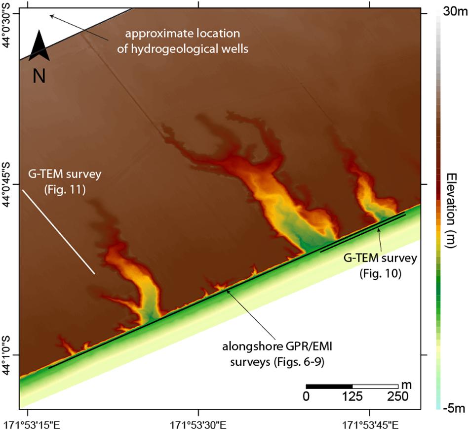
Figure 4. DEM of the study area showing the georeferenced locations of the GPR, EMI, and G-TEM surveys. Approximate locations of the closest hydrogeological wells (∼1 km inland from the coastline) are indicated in the upper left hand corner. The source for the LiDAR data used to produce the DEM is: https://www.linz.govt.nz/.

TABLE 1

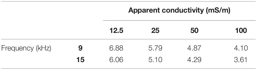
Table 1. Estimated maximum depths of investigation calculated for the range of apparent conductivities measured along the beach at each frequency (units in meters).

EM Surveys

On 5 May 2017 from 11:10 to 11:40 (local time) during high tide (see Table 2), we conducted an alongshore EMI survey using a portable multi-frequency GSSI Profiler EMP-400 to obtain information on the conductivity structure at various depths of investigation (Figure 4). The selected frequencies chosen for this study are 9 and 15 kHz, which correspond to maximum depths of investigation up to 7 m and 6 m, respectively (see Table 1). Although the instrument is capable of recording three frequencies simultaneously, the data of the third channel we collected (3 kHz) was noisy and of poor quality. Herein, we present results from the two higher-frequency channels. The survey locations were chosen to avoid topographic variations alongshore that may adversely affect EMI responses (Santos et al., 2009; Shragge et al., 2017). Measurements were made at 0.5-s intervals using continuous data acquisition mode and the instrument was carried at a constant height of 0.75 m above the ground. All transects were located in the backbeach environment ∼ 25 m inland from the mean tide level. In Section “Results,” we provide a qualitative interpretation of the 9, 15 kHz quadrature responses measured along the shoreline profile. We attempted a laterally constrained, layered inversion of the EMI Profiler data but found that it does not provide useful additional information. A detailed description of the two-layer EMI forward solution and 1D inversion results (see Ward and Hohmann, 1988; Monteiro Santos, 2004; Mester et al., 2011) is given in the Appendix (S1).

TABLE 2

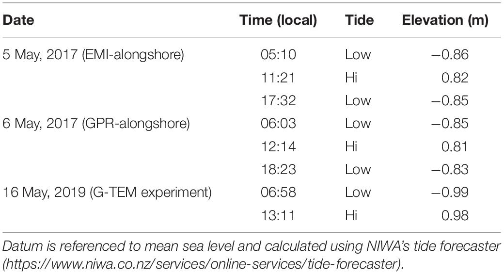
Table 2. Predicted tides at the study site (44° 00′ 58.59″ S, 171° 53′ 21.53″ E) during the duration of the EMI, GPR, and G-TEM experiments.

On May 16, 2019 from 9:12 to 12:10 (local time) during a rising tide, we conducted a 185-m-long G-TEM survey along a shorter segment of the same survey EMI/GPR line previously collected in May, 2017 (Figure 4). The TEM measurements were carried out using the Geonics (Canada) G-TEM system. The G-TEM was operated in an offset-sounding configuration, termed “Slingram” mode in the electromagnetic geophysics literature, in which the RX coil was placed 30 m from the center of the TX loop and the TX-RX pair moved along the transect at 5 m station spacings for 38 stations, maintaining the 30-m offset. Note that the TX and RX are inline for the Slingram configuration, i.e., the line joining the center of the TX loop and the RX coil is aligned with the profile direction. All soundings data were collected in the 20-gate mode with acquisition interval of 6 × 10^–6 s to 8 × 10^–4 s (after ramp-off), corresponding to investigation depths of ∼ 80–100 m. At each station, a consistent 1D smooth inversion model of electrical resistivity vs. depth based on the iterative Occam regularization method (Constable et al., 1987) was performed using the IXG-TEM software from Interpex Limited.

The Slingram configuration was used for the beach profile since no central-loop soundings using the 10 m × 10 m square loop measured on the beach could be fit by a 1D model. An example of a typical 10 m × 10 m central-loop sounding and the best 1D model response showing ∼ 200% root mean square (RMS) misfit is shown in Figure 5A. The four different symbols in Figure 5 represent the four repetitions of a sounding. We repeated each measurement four times in order to estimate the scatter in the response. In low-noise environments, all four sets of data should sit on top of each other, but if there is noise (e.g., random, ambient EM noise from the atmosphere, water waves and currents, or from anthropogenic activity) there will be some scatter. The scatter is especially prominent at the later time gates where the signal from the deep eddy currents in the ground has become small. The poor fit of the central-loop soundings in Figure 5A is likely due to the strong heterogeneity generated by highly contrasting electrical conductivity zones at shallow depths beneath the beach. These contrasts could be related to freshwater discharging into seawater-saturated sediments. The deeper-probing Slingram soundings, on the other hand, could be fit quite well by a 1D model. A representative example with RMS ∼ 22% is shown in (Figure 5B). While we acquired many 10 m × 10 m central loop soundings on the plains above the coastal bluffs, also none of them could be fit by a 1D model, again indicating strong electrical heterogeneity at shallow depths. Interestingly, all soundings made along a plains transect comprised of 40 m × 40 m central loop soundings (described further below) could be fit by a 1D model, a representative example with RMS ∼ 18% is shown in (Figure 5C). To summarize, none of the 10 m × 10 m central-loop soundings made either at the beach or on the adjacent plains could be fit by a 1D model. In contrast, all of the Slingram soundings on the beach and all of the 40 m × 40 m central-loop soundings on the plains could be fit by a 1D model. The implication is that the Slingram configuration is not as sensitive to the strong, shallow variations in electrical conductivity that are picked up by the central loop soundings. While Slingram is deeper probing, it appears that the near-surface is less well resolved with Slingram than it is with the central-loop configuration.

FIGURE 5

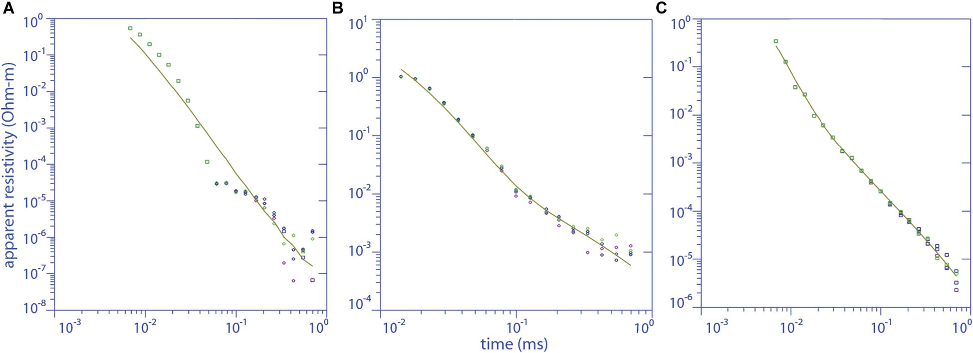
Figure 5. Representative data fits to the G-TEM sounding curves for (A) 10 m × 10 m central-loop sounding on the beach, (B) 10 m × 10 m, and (C) 40 m × 40 m central-loop soundings inland from the bluffs. The dots are the data and the lines are the model fits. Square symbols represent positive responses, whereas negative responses are displayed as diamond symbols. A change in sign in response is due to a change in sign of the vertical magnetic flux passing through the RX coil; such a sign-change is indicative of 2D or 3D structure since the magnetic flux of a transmitted eddy current diffusing into a 1D Earth must maintain the same sign at the center of the RX coil throughout the entire measurement time-window. The symbols are the measured data and the lines represent the best smooth-model response. Different symbols represent different repetitions of the sounding.

GPR Surveys

On 6 May 2017 we conducted an alongshore GPR survey along the identical EMI profile collected the previous day (see Figures 3, 4). The survey line was divided into four shorter transects (Profiles A-D), mainly because of the 12 V battery limitations for both the TX-RX antennae. A 300-m-long line, for example, took 2 h to acquire. The surveys commenced at 10:30 (local time) and ended at 16:50 corresponding to a rising tide and low tide, respectively (Table 2). We used a Sensors & Software pulseEKKO Pro system and acquired data using reflection mode for each transect. Data were collected with a 100 MHz antenna and 1000 V transmitter with an antenna separation of 1 m and a step-size of 0.5 m (see Jol and Bristow, 2003; Neal, 2004). The instrument settings and configuration resulted in a depth of investigation of up to 9 m, which is comparable, but slightly greater than the depth of investigation of the EMI Profiler at 9 kHz (see Table 1). A survey grade GPS with a positional accuracy of 10 cm was used to collocate measurements between the EMI/GPR surveys.

The data were processed using Sensors & Software EKKO_Project processing software. Minimal processing was applied to the data and follows standard GPR processing steps including; Dewow filter, Background Subtraction, and Automatic Gain Control with a maximum gain value of 250, followed by migration (see Neal, 2004; Jol, 2008). The migration velocity was determined through hyperbolic velocity analysis, rather than common midpoint analysis. Hyperbolic matching can be performed on radar sections that contain diffraction or reflection hyperbola and is accomplished by matching the ideal form of a velocity-specified hyperbolic function to the form of the observed data (Jol, 2008). In most cases, the fitted diffraction hyperbola for each GPR line corresponds to a velocity of 0.3 m/ns, which is surprising as this value is the airwave velocity. This value is much higher than values of ∼ 0.1 m/ns normally found in gravel deposits (e.g., McCuaig and Ricketts, 2004; Neal, 2004). The high-porosity gravel at the study site is likely to be highly aerated due to air pressure changes within the vadose zone caused by tide-induced airflow (Jiao and Li, 2004; Jiao and Post, 2019). When the water table rises in response to rising tide the air pressure increases in the vadose zone and air is forced out of the ground. This ventilation, or “breathing” phenomenon is then reversed during a falling tide and air is drawn into the vadose zone. It is reasonable to expect that this process is pronounced in unconsolidated and undersaturated high-porosity gravels in a meso-tidal tide regime. With the exception of the first GPR Line A, all subsequent surveys were conducted during a falling tide (Table 2), thus the increased air within the gravel pore space could drive the GPR electromagnetic wave velocity (see Neal, 2004) close to the 0.3 m/ns value.

Results

A primary research question in this study is to determine whether gravel lenses within the braided alluvial deposits beneath the Canterbury plain are groundwater conduits, potentially discharging offshore. To address this question, we compare results from collocated EMI, GPR, and G-TEM surveys conducted on the beachfront, along with a DEM of the study area (Land Information New Zealand [LINZ], 2019). Complicating our exploration efforts, especially at shallow depths (e.g., <10 m), is the effect of changing tides on the EM signals that we attempted to mitigate by conducting the surveys as far away as possible from the swash zone and by performing a series of calibration tests following the same procedure, as described in Weymer et al. (2016), to gain better insight on interpreting the geophysical results.

Profile A is located at the southernmost section of the survey line and is the shortest GPR profile (117-m long) collected during the field experiment (Figure 6). The GPR data show nearly horizontal reflectors from the surface to a depth of 3 m that we interpret as the signature of the sorted gravels that outcrop on the beach. The basis for our interpretation follows the radar facies classification for comparable paraglacial deposits in southwest British Columbia, Canada by Ékes and Hickin (2001, p. 205). The GPR signal fades between depths of ∼ 3–9 m, and is strongly attenuated below 9 m. As previously mentioned, the survey was conducted along the backbeach, close to the cliffs. The difference in elevation from the backbeach to the swash zone is roughly 2–3 m; thus, the fading GPR signal may correspond to the landward encroachment of seawater. The freshwater/saltwater interface is delineated by the deep, strong reflector that varies with depth. The reflector rises, or is absent, in zones that appear to have a close spatial association with the locations of the box canyons. With respect to the EMI measurements, the signals at 9 and 15 kHz are relatively stable and gradually decrease along the profile. The solid lines in the figure on the EMI-response plots are two-layer model responses showing that a two-layer model fits the data quite well (refer to S1 for more details). There is a pronounced local maximum in both the EMI responses about midway along the profile that is coincident with a major disruption in the strong GPR reflector. More subdued local maxima, especially evident in the 15 kHz signal, appear to correspond albeit less precisely to other disruptions in the strong GPR reflector near the start and end of the profile.

FIGURE 6

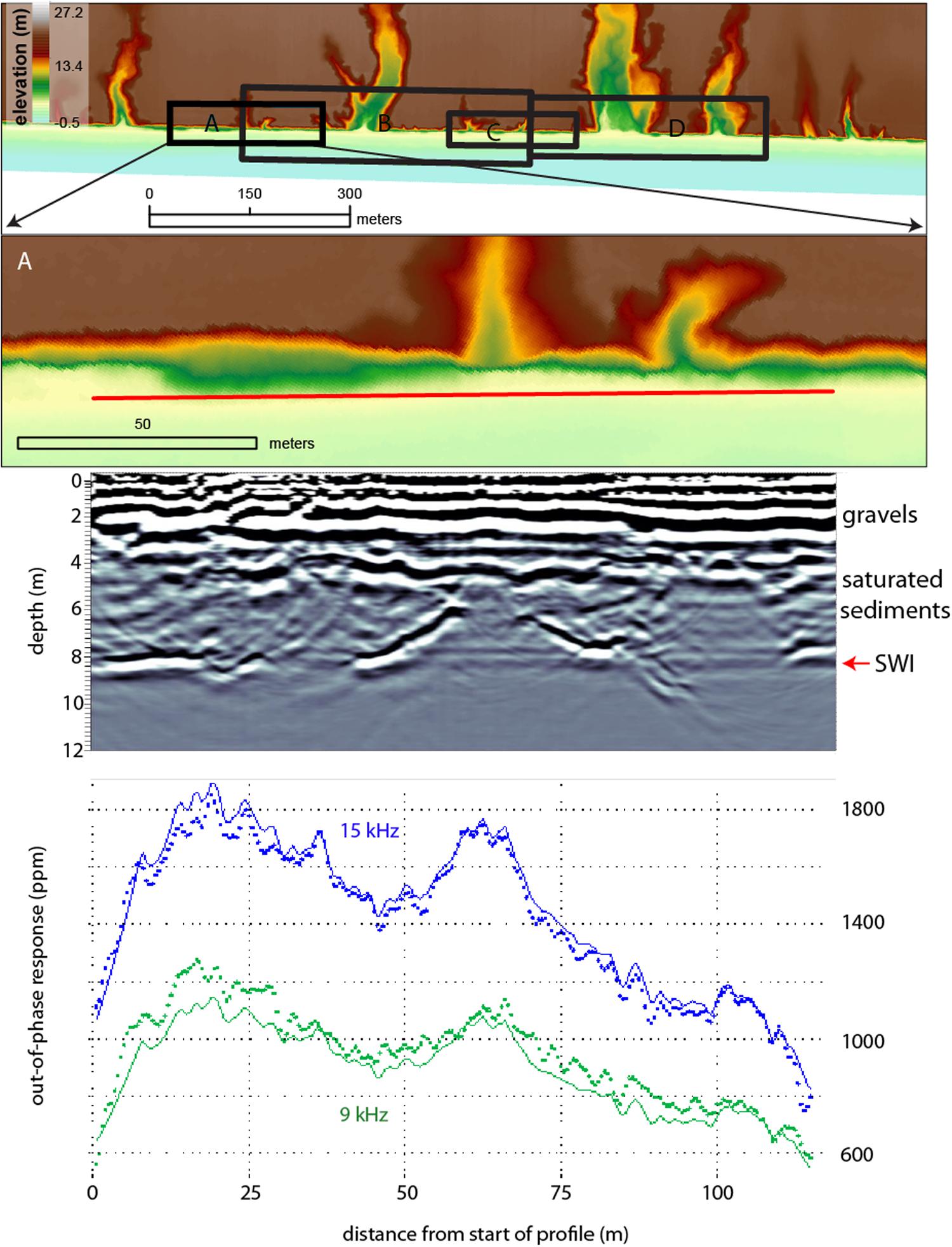
Figure 6. Collocated alongshore GPR and EMI surveys indicated by the red line on each DEM shown in Figures 6–9. Each depth-converted radar section is shown in the middle panel. Measured EMI data (bottom panel) are indicated by the blue and green dots while the solid lines are the fitted data from the 1D inversion. In each figure the freshwater–seawater reflector is denoted by the red arrow marked SWI (saltwater interface) and the approximate depths of the interpreted gravels and saturated sediments are labeled on the right hand side of the GPR section.

The results from Profile B are shown in Figure 7. This transect crosses several box canyons of varying size, including one large canyon that appears to have become stabilized due to its mature vegetation cover. The GPR reflectors within the upper 3 m are more variable than those of Profile A. Similarly to Profile A, the radar signal fades below 3 m and is mostly attenuated below 9 m depth. The strong basal reflector exhibits similar characteristics to the strong reflector observed in Profile A, i.e., it is indicative of a strong lateral contrast in the geological structure that has a spatial association with the canyons. The disruption of the strong GPR reflector is most pronounced within the largest of the box canyons between 230 and 250 m alongshore. The EMI signals at 9 and 15 kHz are also variable alongshore. Local maxima in the signals are evident in several places, such as 130–160 m and 390–410 m, which appear to correlate with disruptions in the GPR reflector. In other places, the spatial correlation between the GPR reflector and the EMI signal is not as prominent.

FIGURE 7

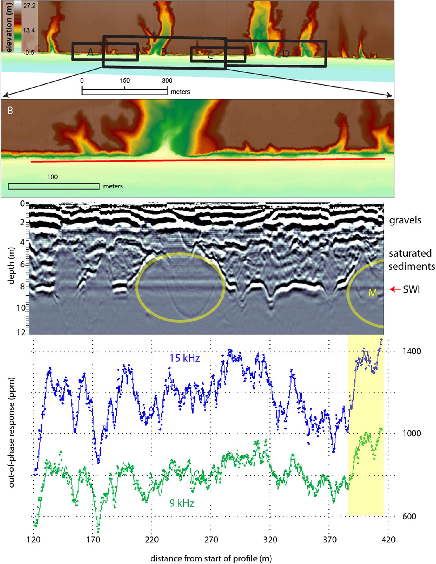
Figure 7. Collocated GPR and EMI survey lines along profile B. Interpreted conduits are marked by yellow circles. Areas where the EMI maxima (highlighted in yellow) match well with the disruption in the radar reflector are marked with an ‘M’ on the GPR section.

The GPR and EMI responses along Profile C are shown in Figure 8. There is one small box canyon on this profile, between distances of ∼ 480–495 m. This is marked by the disruption in the strong GPR reflector, although it should be noted that the signal is not completely disrupted, as it is for some of the box canyons in previous profiles. The highest maximum in the EMI out-of-phase responses occurs at ∼ 470 m, so there is a shift of ∼ 10–15 m in lateral location between the GPR signal disruption and the EMI signal maximum. There is another indication of a break in the GPR reflector near the start of the line that is not clearly associated with a relative maximum in the EMI signals.

FIGURE 8

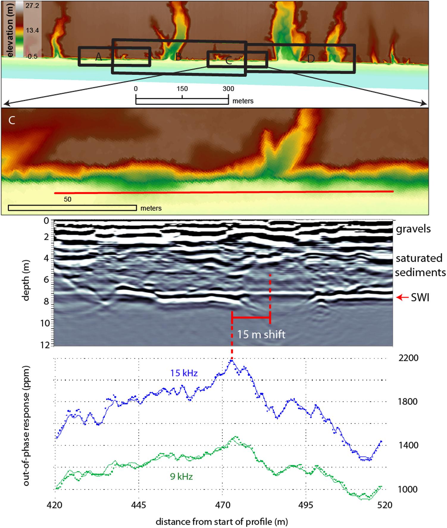
Figure 8. Collocated GPR and EMI survey lines along profile C.

Two large stabilized box canyons with mature vegetation are present on Profile D (Figure 9). Here, the strong GPR reflector is disrupted within both canyons. The EMI signals along this section of the transect are highly variable. There is a pronounced local maximum at locations ∼ 780–800 m that is spatially coincident with a GPR disruption. The largest GPR disruption occurs between stations ∼ 600–670 m. The EMI signals at this location are variable with multiple rises and falls, but a single local maximum is not evident.

FIGURE 9

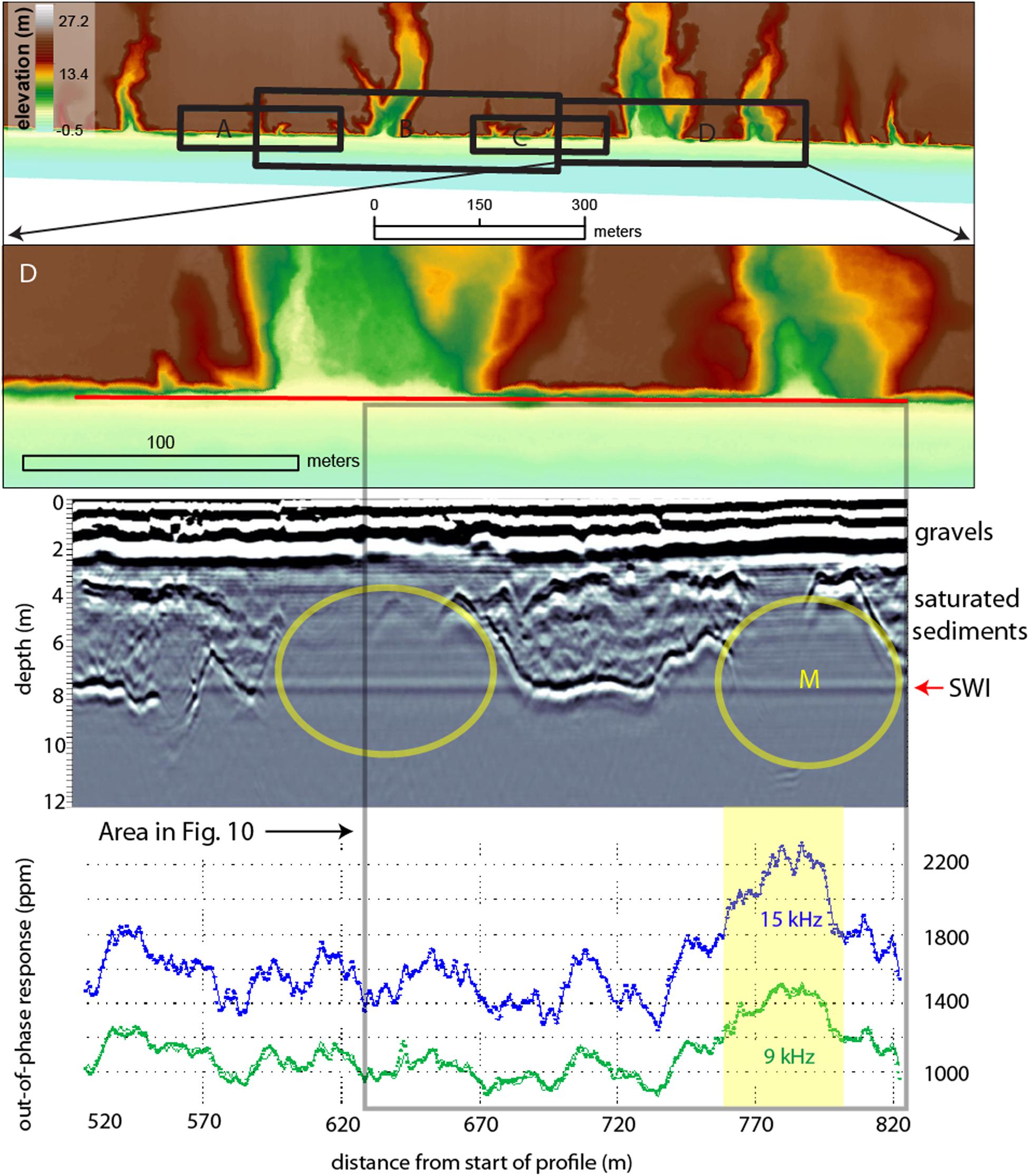
Figure 9. Collocated GPR and EMI survey lines along profile D. Interpreted conduits are marked by yellow circles. Areas where the EMI maxima (highlighted in yellow) match well with the disruption in the radar reflector are marked with an ‘M’ on the GPR section.

A comparison of GPR profile D with a G-TEM transect along the final ∼ 185 m of the same path is shown in Figure 10. The resulting geoelectrical models are shown stitched together in a quasi-2D format in the figure. The G-TEM probes to depths ∼ 80 m, at which low resistivities indicative of clays and/or seawater-saturated sediments ρ ∼ 1–10 Ωm (green-orange-red colors), or high values of conductivity 10–100 mS/m, are found. Above these depths, the ground is more resistive, attaining values up to ρ = 100 Ωm (blue-purple colors), or as low as 1 mS/m conductivity. In the middle part of the section, at depths ∼ 20–30 m, there are a couple of zones that are somewhat less resistive (light blue color), or more conductive, than the surroundings. These zones are indicative of deep alongshore heterogeneity and are discussed below. Note the depth-ranges examined by the GPR (0–9 m) and G-TEM (∼ 10–80 m) in Figure 10 are largely non-overlapping and the near-surface (<10 m depth) structure is not well-resolved by the G-TEM.

FIGURE 10

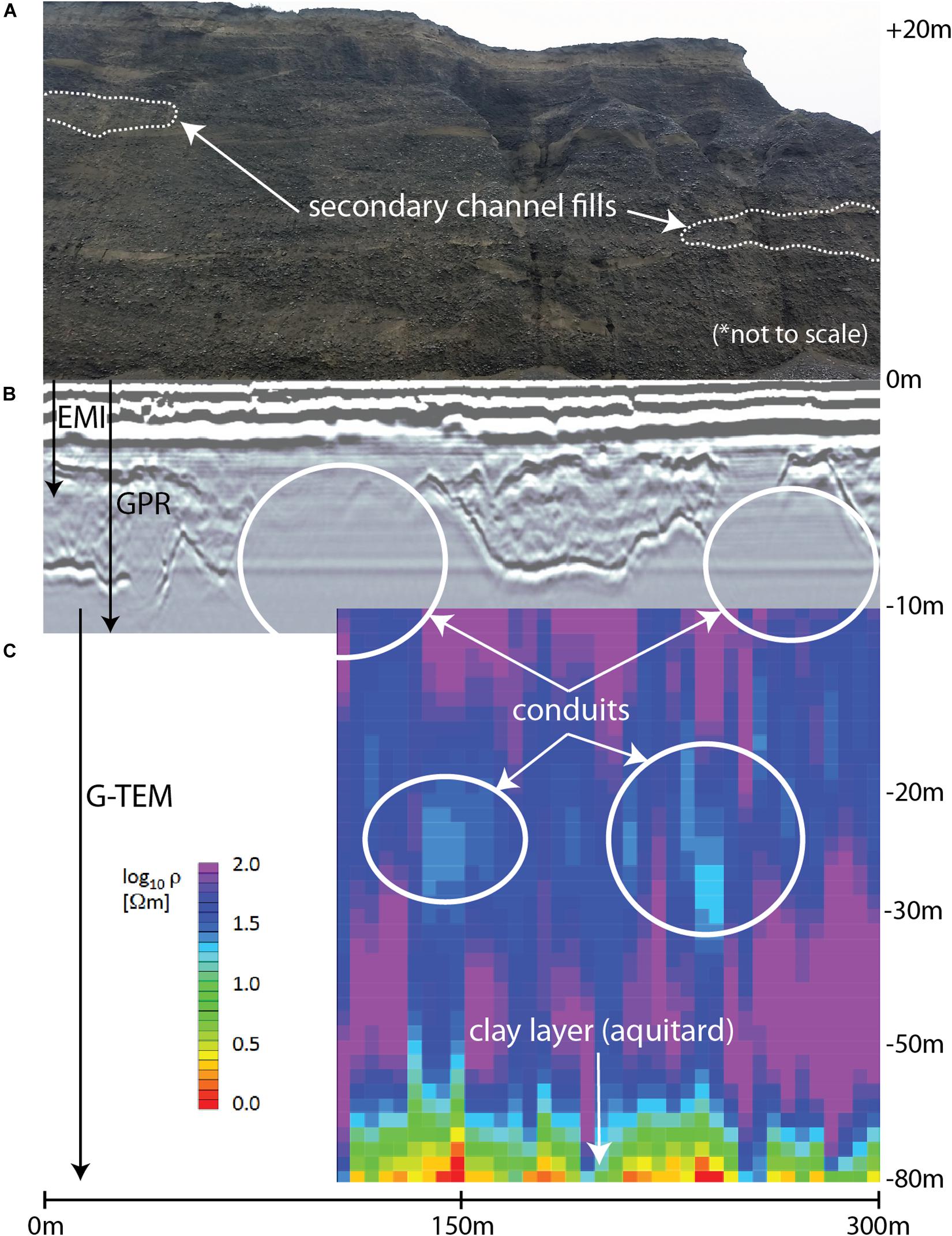
Figure 10. Composite depth slice from the top of the coastal bluff to the maximum depth of investigation probed by the G-TEM system. Secondary channel fills outlined in (A), extending into the subsurface, correspond to conductive zones that are outlined in the GPR section (B) and the inverted G-TEM section (C). Conductive zones illuminate the probable location of groundwater conduits and show evidence for a multilayered system.

To further illustrate that the conductive zones onshore are most likely water-filled gravel conduits, we show an additional coast-normal G-TEM survey (Figure 11). The 40 × 40 m G-TEM 1D stitched section acquired on top of the cliffs (refer to Figure 4) reveals a consistent conductive zone at roughly 7–10 m depths. To test whether the conductive layer is a robust feature of the G-TEM 40 x 40 soundings, we performed a suite of 3-layer forward model calculations. These are summarized in Figure 12. Plotted is the misfit to the G-TEM sounding curve, recorded at the 120 m station location shown in Figure 11, as a function of the resistivity in the depth range of the conductive zone, i.e., 3–15 m. The resistivities of the upper and lower layers were set to 700 Ωm (log₁₀ρ[Ωm] = 2.85) and 415 Ωm (log₁₀ρ[Ωm] = 2.62), respectively, consistent with those shown in Figure 11. It is evident that a middle-zone resistivity of approximately 150 Ωm (log₁₀ρ[Ωm] = 2.15) achieves the lowest misfit, again consistent with Figure 11. A middle-zone resistivity either higher or lower than this value achieves a worse fit, as shown. This modeling exercise demonstrates that the low resistivity of the middle zone is a robust feature of the G-TEM 40 × 40 m soundings and is required by the data.

FIGURE 11

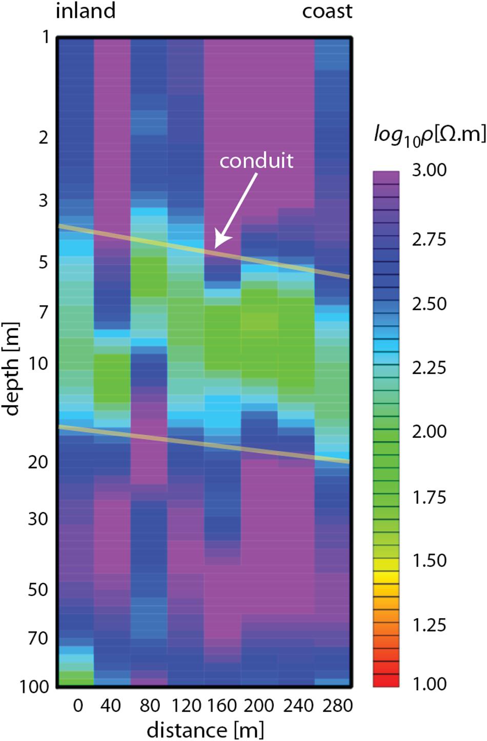
Figure 11. Plot of the 40 × 40 m G-TEM 1D stitched inversion section from the head of the box canyon (0 m) moving inland (280 m). Refer to Figure 4 for the survey location. The interpreted conduit is highlighted in light green colors between the yellow lines.

FIGURE 12

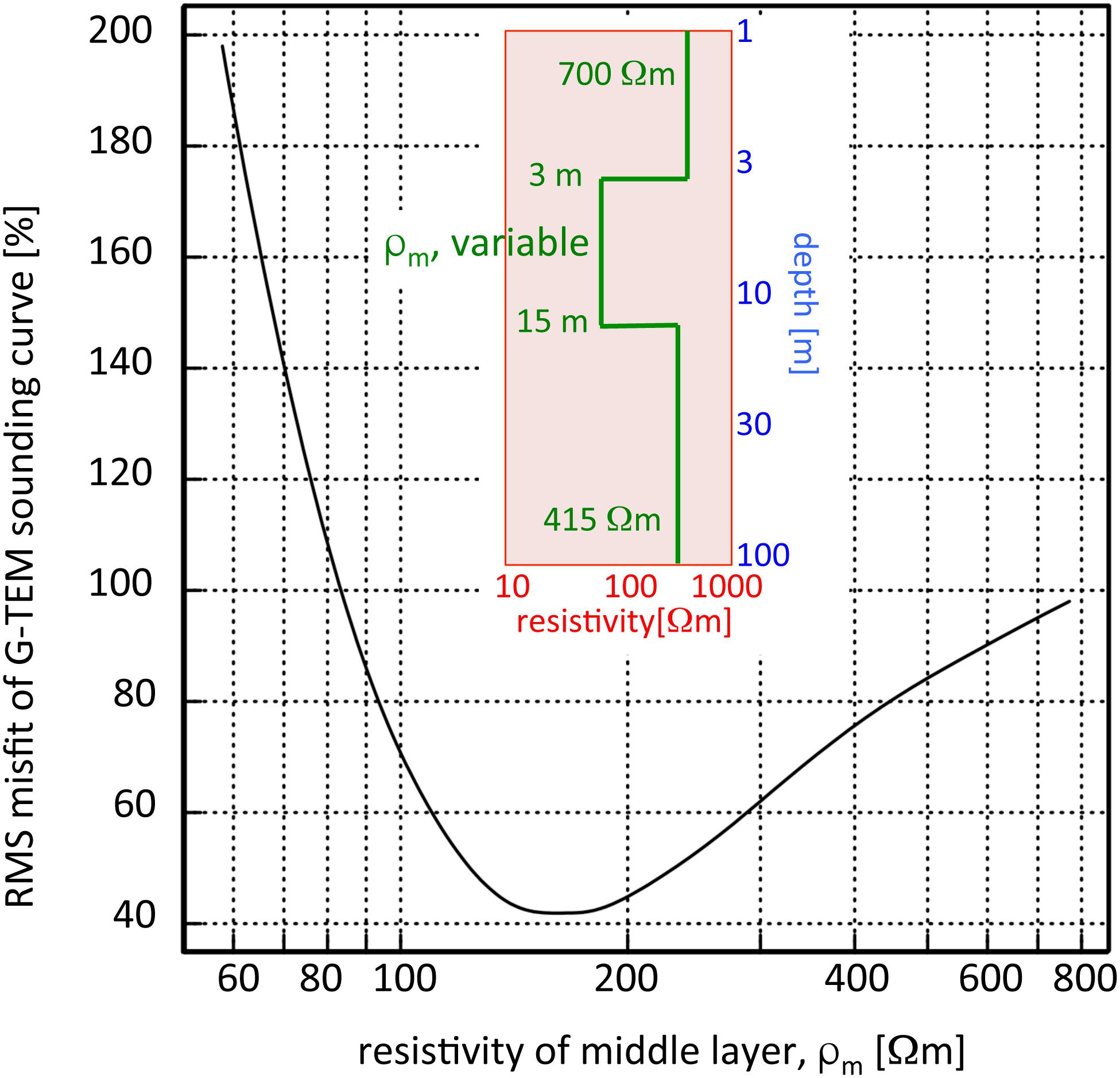
Figure 12. Sensitivity analysis testing the robustness of the conduits observed at the middle sounding station for the G-TEM data shown in Figure 11. The 3-layer model has fixed resistivities of 700 Ωm and 415 Ωm for the upper and lower layers, respectively, whereas the middle layer resistivity is allowed to vary between 60 and 800 Ωm. The resulting curve shows the calculated misfits for the variable resistivities, demonstrating the low resistivity zone (interpreted conduit) having the lowest RMS misfit at ∼ 150 Ωm is a robust feature required by the data.

The resistivity of the conductive layer is about 150 Ωm (green region), or ∼ 7 mS/m conductivity. This value of resistivity is slightly higher than the well water value (see section “High Permeability Sandy Gravels as Groundwater Conduits”), which is to be expected in a coarse sand or gravel matrix since by Archie’s law the effect of the coarse-grained material is to enhance the bulk resistivity relative to that of the well water. Because the conductive layer occurs at each station, at roughly the same depth, this suggests the conduit is continuous and supports the notion of a stream of freshwater discharge toward the coast like a subterranean river. The fact that the 40 × 40 m soundings could be fit by a 1D model, unlike the 10 × 10 central-loop soundings (see section “EM Surveys” and Figure 5), suggests that the deep conductive layer – unlike any shallower conduits – is quite broad, with a width that could be on the order of the instrument footprint. Thus, it is likely there is a considerable volume of deep flowing discharge toward the coast and offshore.

Discussion

In the following, we explore possible scenarios for a discharge model that fits our observations, namely that there is evidence of a multilayered system focusing groundwater flow through stacked high permeability gravel layers analogous to a subterranean river network. First, we discuss the relationships between the sedimentary architecture of the braidplain alluvium and groundwater pathways (Bal, 1996; Moreton et al., 2002). The subsequent sections compare our results with the terrestrial aquifers identified by Davey (2004) and the connection to the OFG system along the Ashburton coast (Micallef et al., 2020).

High Permeability Sandy Gravels as Groundwater Conduits

Quaternary sediments that form the Canterbury Plains consist of sandy gravel aquifers that are characterized by highly variable changes in transmissivities and hydraulic conductivities (Bal, 1996). Wilson (1973) suggests that gravel sorting and increased permeability in the post-glacial alluvium focuses preferred flow paths within “ancient buried river channels” that are recharged by influent seepage from nearby rivers (e.g., Ashburton River). The role of rivers as an important recharge for the Canterbury artesian aquifers has been confirmed in subsequent studies by geochemical (isotopic) and geophysical work (see Bal, 1996). The inherent heterogeneity caused by these preferred flow paths has been described in the literature to vary over a range of spatial scales. As previously mentioned, Bal (1996) identified five to six high permeability corridors (5–10 km wide) east of the Rakaia River that are orders of magnitude larger than the paleochannel conduits suggested by Wilson (1973) where the incised valleys are analogs to “pipelines” or “arteries” containing the discontinuous buried river channels. In contrast, Moreton et al. (2002) suggest high permeability conduits can occur at much smaller spatial scales (tens of meters).

The electromagnetic methods used in this study can diagnose porosity from bulk conductivity σ via Archie’s Law, however, it is important to note that EM methods cannot directly measure permeability, although the two parameters are closely related. The high permeability conduits imaged by the GPR and G-TEM compared to the background geologic matrix (i.e., dry gravels) are generally more conductive. Water conductivity measured in nearby hydrological wells (Environment Canterbury, personal communication), although variable, averages around 30 mS/m, or ∼ 33 Ωm, which in this particular geologic environment is indicative of freshwater-filled gravel conduits. These values are similar to what was measured by the G-TEM (Figure 10) on the beach compared to the background conductivity (∼ 10 mS/m). The results from our EM surveys agree with the findings by Moreton et al. (2002), suggesting that the high permeability conduits occur at smaller spatial scales (Figure 13). However, it is worth noting that our surveys were conducted over a relatively small distance (∼ 800 m) and it is possible that the conduits may increase in size as described by Bal (1996) when investigated at larger spatial scales.

FIGURE 13

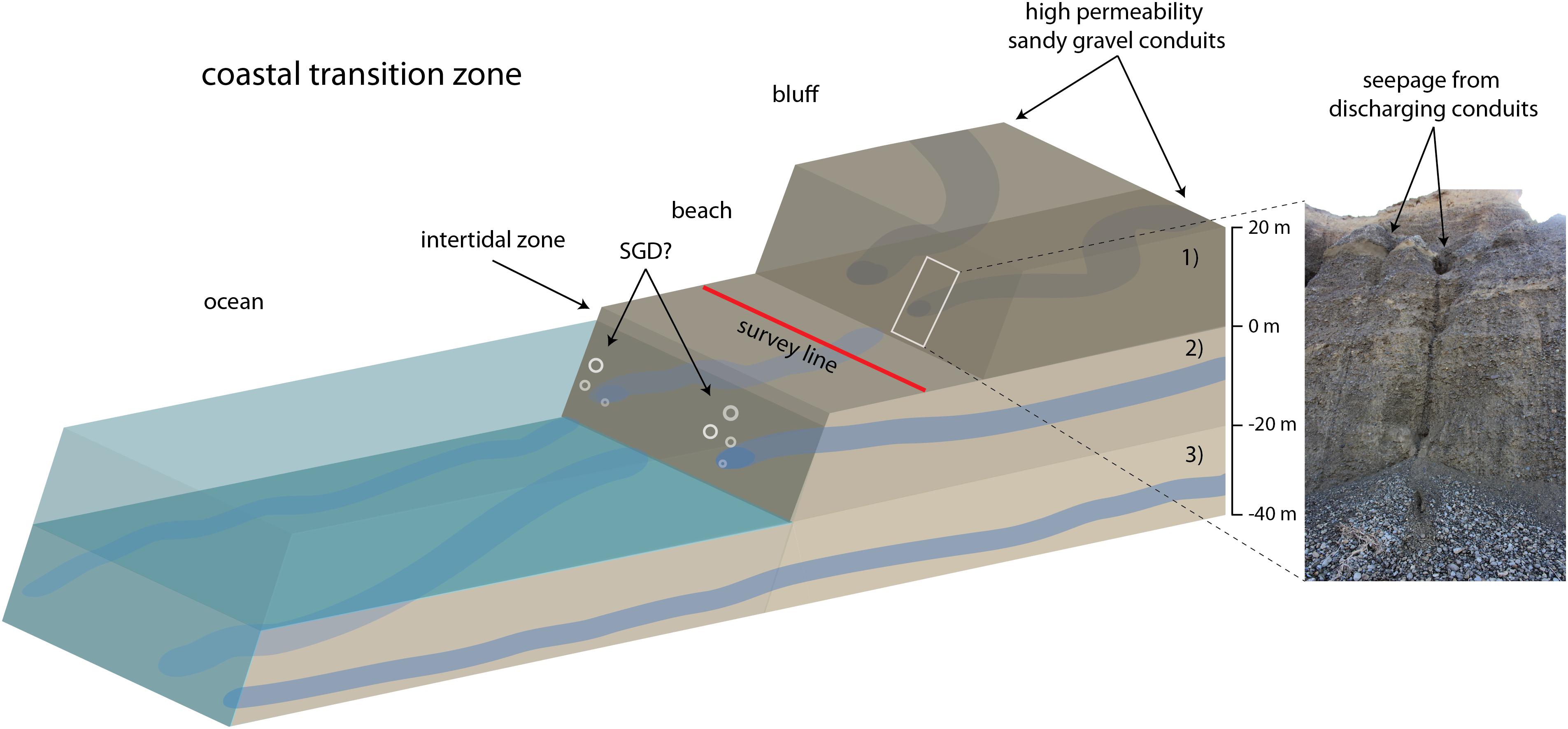
Figure 13. Conceptual discharge model illustrating the configuration of (from top to bottom): (1) high permeability sandy gravel conduits within the coastal bluffs and photograph from the field showing evidence for seepage on the bluff face, (2) shallow conduits in the unconfined aquifer potentially discharging in the nearshore at SGD sites, and (3) deeper conduits connecting the onshore/offshore coastal groundwater system. Approximate depth scale on the right of the right side of the cartoon roughly corresponds to the depths of the conduits in the observed data shown in Figure 10.

Shallow Conduits in the Unconfined Aquifer

In this study, the primary instrument for illuminating potential conduits in the shallow subsurface (≤10 m) is GPR, because the general trend in the EMI signal is essentially consistent across the entire profile and not sensitive to the deeper conductivity structure captured by the GPR and G-TEM. Although local maxima in the EMI signals are evident in several places, which appear to correlate with disruptions in the GPR reflector, other areas are less prominent. The shallow conduits imaged by the GPR at greater depths roughly correspond to the location of the unconfined aquifer identified by Davey (2004). In the following, we explore the possible causes for the reflectors within the GPR signal and their relation to the groundwater conduits.

It is possible that the undulating reflector in GPR profiles along the beach (Figures 6–9) is simply the product of the transmitted signal reflecting off the bluff face. If this were the case, we would expect to see the reflector at ∼ 2–3 m deep, corresponding to the physical distance between the GPR transect and the bluff face (Figure 3). In addition, the reflector should appear deeper when the GPR transect crosses a box canyon because the transmitted signal would take longer to reach the bluff face within a canyon compared to the relatively straight bluff edge. Since the reflector appears deeper (∼ 8 m) than the distance between the survey transect and bluff edge, and the reflector becomes shallower wherever the transect crosses a box canyon, it is unlikely that this strong reflector represents the bluff face. The mismatch between reflector depth, distance to the bluff, and canyon locations suggests that the strong reflector at approximately 8 m depth is not the result of the bluff face reflecting the GPR transmission, but rather a strong contrast in dielectric permittivity ε caused by variations in the subsurface hydrogeology.

Ground penetrating radar has been used to identify lithologic changes in framework geology, which have been suggested to influence the morphodynamics of the beach-dune system (e.g., Riggs et al., 1995). It is possible that the reflector at 8 m depth represents a paleo-channel because its depth varies alongshore. Alongshore variations in subsurface geology, such as infilled paleo-channels and storm washover deposits, have been mapped using GPR along sandy coasts (Weymer et al., 2016; Wernette, 2017). However, unlike previous work, the pronounced reflector along the Ashburton coast becomes shallower as the transect crosses near a box canyon, which suggests a rise in a paleo-topographic surface and contrasts observations using GPR to image paleo-channels in previous research. In addition, the reflector rises more steeply and frequently than dipping reflectors described in the literature. Since the depth of the reflector is opposite of a paleo-channel in direction and there is no evidence of any lithologic discontinuity outcropping at the shoreface or on the larger landscape, it is unlikely that the strong undulating reflector in the GPR profiles represents a paleo-topographic surface or paleo-channel.

Another possible explanation for the undulating reflector in the GPR profiles is that it represents the location of the saltwater-freshwater interface. Contrasting previous investigations in the coastal environment where brackish or saline groundwater has been shown to attenuate the signal (see Jol et al., 1996; Heteren et al., 1998), the GPR data collected along the Ashburton coast has a strong, relatively continuous, and undulating reflector. It is questionable that the saltwater-freshwater interface would appear as a very strong reflector that varies in depth by 5 m within a few meters alongshore multiple times, unless it was accompanied by a prominent lithologic discontinuity, which there was no evidence for on the landscape, or in the nearshore. Given that alongshore variation in the depth of the subsurface reflector is unlikely caused by the bluff reflecting the signal or the saltwater-freshwater interface and probably does not represent a paleo-channel in the subsurface geology, it is feasible that this reflector represents the boundary of concentrated groundwater flows. The contrast between dry, less conductive gravels that appear as concave/convex reflectors and saturated sediments at depth along Profiles B and D (Figures 7, 9) appear as a strong reflector that varies with groundwater saturation. This suggests that the reflectors in the GPR sections and the areas where the GPR signal is attenuated correspond to shallow conduits consisting of lenses of well-sorted gravels and interbedded sands within the braided river deposit architecture (<9 m) that likely discharge at the seafloor close to the coast (Figure 13).

Deeper Conduits Connecting the Onshore/Offshore Coastal Groundwater System

The G-TEM results from the Slingram survey along the coast (Figure 10) reveal two zones at ∼ 20–30 m depth of similar conductivities that were observed in nearby hydrogeological wells (see Figure 4) averaging around 30 mS/m (∼ 33 Ωm). These values are comparable to resistivities measured offshore (Micallef et al., 2020) that were interpreted to indicate the location of the OFG system. The conduits onshore appear as conductive because they are situated in a resistive gravely matrix, whereas the offshore extensions of the conduits manifest as resistors in the offshore imaging because there they are situated in conductive seawater sediments.

Assuming the aquifer is horizontal from the closest boreholes (∼ 1.5 km inland) to the coast and that the elevation at the top of the coastal bluffs is ∼ 20 m, we expect a 20 m offset in observed aquifer depth at the location of our G-TEM survey (at sea level). By comparison, this would assign the depth of the first confining layer (50 m) in Davey (2004) to 30 m in our data. Our data do not appear to show the first confining layer (at least in this particular area) because the conductivities are much lower than what would be expected for a clay layer/aquitard (Figure 10). Thus, we interpret these zones as groundwater conduits within the onshore aquifer system that are focusing flow offshore and are likely connected to the OFG system (Figure 13). The depth of the OFG system interpreted in Micallef et al. (2020) is slightly deeper, occurring at depths of 50 m or more. Marine seismic data (Micallef et al., 2020) show that the gravels extend further offshore in the region directly offshore the Ashburton coast, i.e., the location of the surveys presented in this study. It is probable these gravel channels imaged in the offshore seismic data are connected to the coast, providing evidence for an onshore connection to the conduits/aquifers in the region. The high conductivity zone at 60–70 m is probably the second aquitard described by Davey (2004), but our interpretation is limited in resolution because the maximum depth of investigation of the G-TEM system is 80 m from the TX-RX configuration used in this study.

Our geophysical interpretations support the scale modeling study and field observations from Moreton et al. (2002) in that the conductive zones are most likely caused by freshwater saturated secondary channel fill deposits, which focus groundwater flow offshore. Overall, five key observations can be made: (1) There is a strong GPR reflector that varies with depth and appears to be spatially correlated with large box canyons incised on the coastal bluffs, (2) The GPR signals show consistently high signal attenuation within the larger box canyons and below a depth of ∼ 9 m, (3) EMI σ_a measurements at both frequencies 9 and 15 kHz are surprisingly resistive for a coastal beach environment and do not exceed 60 mS/m over the total length of the survey, (4) The out-of-phase EMI responses are spatially correlated with the strong GPR reflector, and (5) the conductive (∼30 mS/m) zones compared to background (∼10 mS/m) in the inverted G-TEM profiles correspond to the location of large box canyons. Thus, we conclude that the results presented in this study all point to a geologic control within the Canterbury alluvial braidplain that preferentially focuses groundwater flow offshore through high permeability gravels at depths roughly between 20 and 30 m beneath the modern coastline.

Conclusion

This study demonstrates the utility of combining near-surface electromagnetic methods to image groundwater pathways within braided alluvial gravels along the Canterbury coast, South Island, New Zealand. Our results show that collocated EMI, GPR, and G-TEM measurements adequately characterize hydrogeologic variations beneath a mixed sand gravel beach. The combined measurements – providing information at three different depths of investigation and resolution – show several zones of relatively high electrical conductivity compared to the resistive geologic background that are correlated with spatial variations in subsurface hydrogeology. We interpret the conductive zones as high permeability conduits corresponding to lenses of clean, well-sorted gravels interbedded with sands within the braided river deposit architecture. The geophysical surveys provide the basis for a discharge model that fits our observations, namely that there is evidence of a multilayered system focusing groundwater flow through stacked high permeability gravel layers analogous to a subterranean river network.

Our study complements a large-scale geophysical survey conducted offshore along the Canterbury Bight to map OFG systems, for which a meteoric origin and present-day connection to onshore aquifers is inferred. Our results provide evidence that this newly discovered OFG system (Micallef et al., 2020) has been recharged in the past via these conduits and is likely connected to terrestrial aquifers underlying the Canterbury Plains. Our findings have important implications for the potential use of offshore groundwater to alleviate water stress from agriculture/irrigation to one of the driest regions in New Zealand. The geology of the New Zealand coast is quite heterogeneous and geoelectrically 3D, yet the EM instruments used in this study are capable of detecting variations in the subsurface hydrogeology. It is reasonable to expect that the combined EM methods presented in this study could also be applied in other coastal geologic settings, e.g., carbonate platforms, barrier islands, volcanic islands.

Although our work is suggestive of groundwater conduits discharging offshore, we emphasize that this is a working hypothesis until more testing is done in the future. Given the large spatial disconnect between the terrestrial surveys of this paper and offshore controlled-source electromagnetic surveys (Micallef et al., 2020), it is yet unclear how these groundwater conduits may relate to broader variations in coastal groundwater dynamics. Moving forward, we propose that EM geophysics offers exciting new opportunities in bridging the gap across the coastal transition zone using, for example; airborne electromagnetics, autonomous underwater vehicles (AUVs), surface wave gliders, unoccupied aerial vehicles (UAVs) and potentially other platforms. Future work should seek to (1) map the conduits across the ‘White Ribbon’ and offshore in high resolution, (2) understand how onshore groundwater conduits evolve on a variety of spatiotemporal scales, and (3) quantify the volume and flux of terrestrial groundwater to the sub-ocean reservoir caused in part by variations in local and regional geology.

Data Availability Statement

All datasets generated for this study are included in the article/Supplementary Material, and can be made available by contacting the corresponding author: brad.weymer@gmail.com.

Author Contributions

BW and PW set up and designed the study for the 2017 field surveys. BW prepared the manuscript with contributions from all co-authors. BW processed the GPR data and PW helped merge the DEMs and EMI profiles for Figures 6–9. ME, PP, and AM collected the G-TEM data during the 2019 field campaign. ME performed the inversion. ME, PP, and MJ contributed to the discussion on the inversion results. All authors contributed to the article and approved the submitted version.

Funding

This project has received funding from the European Research Council (ERC) under the European Union’s Horizon 2020 Research and Innovation Programme (Grant Agreement No. 677898; MARCAN). This research was also funded in part by the SMART Project through the Helmholtz European Partnering Initiative (Project ID Number PIE-0004).

Conflict of Interest

The authors declare that the research was conducted in the absence of any commercial or financial relationships that could be construed as a potential conflict of interest.

Acknowledgments

We are grateful to Robbie Bennet for kindly allowing us to conduct our field surveys on his farm. We thank Daniele Spatola and Daniel Cuñarro Otero for their assistance in the field in May 2017. All data in this study are available by contacting the corresponding author: brad.weymer@gmail.com.

Supplementary Material

The Supplementary Material for this article can be found online at: https://www.frontiersin.org/articles/10.3389/fmars.2020.531293/full#supplementary-material

References

Archie, G. E. (1942). The electrical resistivity log as an aid in determining some reservoir characteristics. Trans. AIME 146, 54–62. doi: 10.2118/942054-g

PubMed Abstract | CrossRef Full Text | Google Scholar

Ashworth, P. J., Best, J. L., Peakall, J., Lorsong, J. A., Smith, N. D., and Rogers, J. (1999). The influence of aggradation rate on braided alluvial architecture: field study and physical scale-modelling of the Ashburton River gravels, Canterbury Plains, New Zealand. Fluvial Sedimentol. 6, 331–346. doi: 10.1002/9781444304213.ch24

CrossRef Full Text | Google Scholar

Badea, E. A., Everett, M. E., Newman, G. A., and Biro, O. (2001). Finite-element analysis of controlled-source electromagnetic induction using Coulomb-gauged potentials. Geophysics 66, 786–799. doi: 10.1190/1.1444968

CrossRef Full Text | Google Scholar

Bailey, S., and Bristow, C. S. (2000). “Structure of coastal dunes: observations from ground penetrating radar (GPR) surveys,” in Proceedings of the Eighth International Conference on Ground Penetrating Radar. International Society for Optics and Photonics, Gold Coast, 660–665.

Google Scholar

Bal, A. A. (1996). Valley fills and coastal cliffs buried beneath an alluvial plain: evidence from variation of permeabilities in gravel aquifers, Canterbury Plains, New Zealand. J. Hydrol. 35, 1–27.

Google Scholar

Barlow, P. M. (2003). Ground Water in Freshwater-Saltwater Environments of the Atlantic Coasti > (Vol. 1262). Reston: Geological Survey (USGS).

Google Scholar

Berger, G. W., Tonkin, P. J., and Pillans, B. (1996). Thermo-luminescence ages of post-glacial loess, Rakaia River, South Island, New Zealand. Q. Int. 35, 177–182. doi: 10.1016/1040-6182(95)00082-8

CrossRef Full Text | Google Scholar

Berndt, C., and Micallef, A. (2019). Could offshore groundwater rescue coastal cities? Nature 574:36. doi: 10.1038/d41586-019-02924-7

PubMed Abstract | CrossRef Full Text | Google Scholar

Bratton, J. F. (2010). The three scales of submarine groundwater flow and discharge across passive continental margins. J. Geol. 118, 565–575. doi: 10.1086/655114

CrossRef Full Text | Google Scholar

Browne, G. H., and Naish, T. R. (2003). Facies development and sequence architecture of a late Quaternary fluvial-marine transition, Canterbury Plains and shelf, New Zealand: implications for forced regressive deposits. Sediment. Geol. 158, 57–86. doi: 10.1016/s0037-0738(02)00258-0

CrossRef Full Text | Google Scholar

Burnett, W., Aggarwal, P., Aureli, A., Bokuniewicz, H., Cable, J., Charette, M., et al. (2006). Quantifying submarine groundwater discharge in the coastal zone via multiple methods. Sci. Total Environ. 367, 498–543.

Google Scholar

Cohen, D., Person, M., Wang, P., Gable, C. W., Hutchinson, D., Marksamer, A., et al. (2010). Origin and extent of fresh paleowaters on the Atlantic continental shelf, USA. Groundwater 48, 143–158. doi: 10.1111/j.1745-6584.2009.00627.x

PubMed Abstract | CrossRef Full Text | Google Scholar

Constable, S. C., Parker, R. L., and Constable, C. G. (1987). Occam’s inversion: a practical algorithm for generating smooth models from electromagnetic sounding data. Geophysics 52, 289–300. doi: 10.1190/1.1442303

CrossRef Full Text | Google Scholar

Davey, G. (2004). Aquidef, a MS Access Programme to Define Canterbury Plains Aquifers and Aquitards. Environmental Canterbury Technical Report, No. U04/42.

Google Scholar

Davey, G. (2006). Definition of the Canterbury Plains aquifers. Environmental Canterbury Technical Report, No. U06/10.

Google Scholar

Davies, J. L. (1964). A morphogenetic approach to world shore-lines. Z. Geomorphol. 8, 127–142.

Google Scholar

Delefortrie, S., Saey, T., Van De Vijver, E., De Smedt, P., Missiaen, T., Demerre, I., et al. (2014). Frequency domain electromagnetic induction survey in the intertidal zone: limitations of low-induction-number and depth of exploration. J. Appl. Geophys. 100, 14–22. doi: 10.1016/j.jappgeo.2013.10.005

CrossRef Full Text | Google Scholar

Ékes, C., and Hickin, E. J. (2001). Ground penetrating radar facies of the paraglacial Cheekye Fan, southwestern British Columbia, Canada. Sediment. Geol. 143, 199–217. doi: 10.1016/s0037-0738(01)00059-8

CrossRef Full Text | Google Scholar

Evans, R. L. (2007). Using CSEM techniques to map the shallow section of seafloor: from the coastline to the edges of the continental slope. Geophysics 72, WA105–WA116.

Google Scholar

Evans, R. L., and Lizarralde, D. (2011). The competing impacts of geology and groundwater on electrical resistivity around Wrightsville Beach, NC. Continent. Shelf Res. 31, 841–848. doi: 10.1016/j.csr.2011.02.008

CrossRef Full Text | Google Scholar

Everett, M. E. (2013). Near-Surface Applied Geophysics. Cambridge, MA: Cambridge Univ. Press.

Google Scholar

Everett, M. E., and Chave, A. D. (2019). On the physical principles underlying electromagnetic induction. Geophysics 84, W21–W32.

Google Scholar

Ferguson, G., and Gleeson, T. (2012). Vulnerability of coastal aquifers to groundwater use and climate change. Nat. Clim. Change 2, 342–345. doi: 10.1038/nclimate1413

CrossRef Full Text | Google Scholar

Fitterman, D. V. (2015). Tools and techniques: active-source electromagnetic methods, in < /i > l. slater (ed.), resources in the near-surface earth. < /i >. Treatise Geophys. 11, 295–333. doi: 10.1016/b978-0-444-53802-4.00193-7

CrossRef Full Text | Google Scholar

Gustafson, C., Key, K., and Evans, R. L. (2019). Aquifer systems extending far offshore on the US Atlantic margin. Sci. Rep. 9, 1–10. doi: 10.1130/dnag-gna-i2.1

CrossRef Full Text | Google Scholar

Heath, R. A. (1981). Oceanic fronts around southern New Zealand. Deep Sea Res. A Oceanogr. Res. Pap. 28, 547–560. doi: 10.1016/0198-0149(81)90116-3

CrossRef Full Text | Google Scholar

Heteren, S. V., Fitzgerald, D. M., Mckinlay, P. A., and Buynevich, I. V. (1998). Radar facies of paraglacial barrier systems: coastal New England, USA. Sedimentology 45, 181–200. doi: 10.1046/j.1365-3091.1998.00150.x

CrossRef Full Text | Google Scholar

Huang, H., and Won, I. J. (2000). Conductivity and susceptibility mapping using broadband electromagnetic sensors. J. Environ. Eng. Geophys. 5, 31–41. doi: 10.4133/jeeg5.4.31

CrossRef Full Text | Google Scholar

Jennings, R., and Shulmeister, J. (2002). A field based classification scheme for gravel beaches. Mar. Geol. 186, 211–228. doi: 10.1016/s0025-3227(02)00314-6

CrossRef Full Text | Google Scholar

Jiao, J., and Post, V. (2019). Coastal Hydrogeology. Cambridge, MA: Cambridge University Press.

Google Scholar

Jiao, J. J., and Li, H. (2004). Breathing of coastal vadose zone induced by sea level fluctuations. Geophys. Res. Lett. 31:L11502.

Google Scholar

Johannes, R. E. (1980). Ecological significance of the submarine discharge of groundwater. Mar. Ecol. Prog. Ser. 3, 365–373. doi: 10.3354/meps003365

CrossRef Full Text | Google Scholar

Johnston, R. H. (1983). The saltwater-freshwater interface in the Tertiary limestone aquifer, southeast Atlantic outer-continental shelf of the USA. J. Hydrol. 61, 239–249. doi: 10.1016/0022-1694(83)90251-2

CrossRef Full Text | Google Scholar

Jol, H. M. (2008). Ground Penetrating Radar Theory and Applications. Amsterdam: Elsevier.

Google Scholar

Jol, H. M., and Bristow, C. S. (2003). GPR in sediments: advice on data collection, basic processing and interpretation, a good practice guide. Geol. Soc. Lond. Spec. Publ. 211, 9–27. doi: 10.1144/gsl.sp.2001.211.01.02

CrossRef Full Text | Google Scholar

Jol, H. M., Smith, D. G., and Meyers, R. A. (1996). Digital ground penetrating radar (GPR): a new geophysical tool for coastal barrier research (examples from the Atlantic, Gulf and Pacific Coasts, USA). J. Coast. Res. 12, 960–968.

Google Scholar

Kirk, R. M. (1980). Mixed sand and gravel beaches: morphology, processes and sediments. Prog. Phys. Geogr. 4, 189–210. doi: 10.1177/030913338000400203

CrossRef Full Text | Google Scholar

Land Information New Zealand [LINZ] (2019). Available online at: https://www.linz.govt.nz/ (accessed November 26, 2019).

Google Scholar

Leckie, D. A. (2003). Modern environments of the Canterbury Plains and adjacent offshore areas, New Zealand—an analog for ancient conglomeratic depositional systems in nonmarine and coastal zone settings. Bull. Can. Petrol. Geol. 51, 389–425. doi: 10.2113/51.4.389

CrossRef Full Text | Google Scholar

Leon, J. X., Phinn, S. R., Hamylton, S., and Saunders, M. I. (2013). Filling the ‘white ribbon’–a multisource seamless digital elevation model for Lizard Island, northern Great Barrier Reef. Int. J. Remote Sens. 34, 6337–6354. doi: 10.1080/01431161.2013.800659

CrossRef Full Text | Google Scholar

Mandel, S. (1974). The Groundwater Resources of the Canterbury Plains. Canterbury: Lincoln University.

Google Scholar

McCuaig, S. J., and Ricketts, M. J. (2004). Ground-probing radar as a tool for heterogeneity estimation in gravel deposits: advances in data-processing and facies analysis. Curr. Res. Newf. Dept. Mines Energy Geol. Surv. Rep. 4, 107–115.

Google Scholar

McLean, R. F. (1970). Variations in grain-size and sorting on two kaikoura beaches. New Zealand J. Mar. Freshw. Res. 4, 141–164. doi: 10.1080/00288330.1970.9515334

CrossRef Full Text | Google Scholar

Mester, A., van der Kruk, J., Zimmermann, E., and Vereecken, H. (2011). Quantitative two-layer conductivity inversion of multi-configuration electromagnetic induction measurements. Vadose Zone J. 10, 1319–1330. doi: 10.2136/vzj2011.0035

CrossRef Full Text | Google Scholar

Micallef, A., Person, M., Haroon, A., Weymer, B. A., Jegen, M., Schwalenberg, K., et al. (2020). 3D characterisation and quantification of an offshore freshened groundwater system in the Canterbury Bight, New Zealand. Nat. Commun. 11:1372.

Google Scholar

Michael, H. A., Post, V. E., Wilson, A. M., and Werner, A. D. (2017). Science, society, and the coastal groundwater squeeze. Water Resour. Res. 53, 2610–2617. doi: 10.1002/2017wr020851

CrossRef Full Text | Google Scholar

Monteiro Santos, F. A. (2004). 1-D laterally constrained inversion of EM34 profiling data. J. Appl. Geophys. 56, 123–134. doi: 10.1016/j.jappgeo.2004.04.005

CrossRef Full Text | Google Scholar

Moore, W. S. (1996). Large groundwater inputs to coastal waters revealed by 226Ra enrichments. Nature 380, 612–614. doi: 10.1038/380612a0

CrossRef Full Text | Google Scholar

Moore, W. S. (1999). The subterranean estuary: a reaction zone of ground water and sea water. Mar. Chem. 65, 111–125. doi: 10.1016/s0304-4203(99)00014-6

CrossRef Full Text | Google Scholar

Moore, W. S. (2010). The effect of submarine groundwater discharge on the ocean. Annu. Rev. Mar. Sci. 2, 59–88.

Google Scholar

Moosdorf, N., and Oehler, T. (2017). Societal use of fresh submarine groundwater discharge: an overlooked water resource. Earth Sci. Rev. 171, 338–348. doi: 10.1016/j.earscirev.2017.06.006

CrossRef Full Text | Google Scholar

Moreton, D. J., Ashworth, P. J., and Best, J. L. (2002). The physical scale modelling of braided alluvial architecture and estimation of subsurface permeability. Basin Res. 14, 265–285. doi: 10.1046/j.1365-2117.2002.00189.x

CrossRef Full Text | Google Scholar

Nabighian, M. N., and Macnae, J. C. (1991). Time domain electromagnetic prospecting methods. Electromagn. Methods Appl. Geophys. 2(part A), 427–509. doi: 10.1190/1.9781560802686.ch6

CrossRef Full Text | Google Scholar

Neal, A. (2004). Ground-penetrating radar and its use in sedimentology: principles, problems and progress. Earth Sci. Rev. 66, 261–330. doi: 10.1016/j.earscirev.2004.01.004

CrossRef Full Text | Google Scholar

Palacky, G. J. (1988). Resistivity characteristics of geologic targets. Electromagn. Methods Appl. Geophys. 1, 53–129.

Google Scholar

Person, M., Dugan, B., Swenson, J. B., Urbano, L., Stott, C., Taylor, J., et al. (2003). Pleistocene hydrogeology of the Atlantic continental shelf, New England. Geol. Soc. Am. Bull. 115, 1324–1343. doi: 10.1130/b25285.1

CrossRef Full Text | Google Scholar

Person, M., McIntosh, J., Bense, V., and Remenda, V. H. (2007). Pleistocene hydrology of North America: the role of ice sheets in reorganizing groundwater flow systems. Rev. Geophys. 45:RG3007.

Google Scholar

Post, V. (2005). Fresh and saline groundwater interaction in coastal aquifers: is our technology ready for the problems ahead? Hydrogeol. J. 13, 120–123. doi: 10.1007/s10040-004-0417-2

CrossRef Full Text | Google Scholar

Post, V. E., Groen, J., Kooi, H., Person, M., Ge, S., and Edmunds, W. M. (2013). Offshore fresh groundwater reserves as a global phenomenon. Nature 504:71. doi: 10.1038/nature12858

PubMed Abstract | CrossRef Full Text | Google Scholar

Post, V. E. A., Eichholz, M., and Brentführer, R. (2018). Groundwater Management in Coastal Zones. Hannover: Bundesanstalt für Geowissenschaften und Rohstoffe (BGR).

Google Scholar

Riggs, S. R., Cleary, W. J., and Snyder, S. W. (1995). Influence of inherited geologic framework on barrier shoreface morphology and dynamics. Mar. Geol. 126, 213–234. doi: 10.1016/0025-3227(95)00079-e

CrossRef Full Text | Google Scholar

Ryan, W. B., Carbotte, S. M., Coplan, J. O., O’Hara, S., Melkonian, A., Arko, R., et al. (2009). Global multi-resolution topography synthesis. Geochem. Geophys. Geosyst. 10:Q03014.

Google Scholar

Santos, V. R., Porsani, J. L., Mendonça, C. A., Rodrigues, S. I., and DeBlasis, P. D. (2009). Reduction of topography effect in inductive electromagnetic profiles: application on coastal sambaqui (shell mound) archaeological site in Santa Catarina state, Brazil. J. Archaeol. Sci. 36, 2089–2095. doi: 10.1016/j.jas.2009.05.014

CrossRef Full Text | Google Scholar

Schumm, S., and Phillips, L. (1986). Composite channels of the Canterbury Plain, New Zealand: a martian analog? Geology 14, 326–329. doi: 10.1130/0091-7613(1986)14<326:ccotcp>2.0.co;2

CrossRef Full Text | Google Scholar

Shragge, J., Lumley, D., Issa, N., Hoskin, T., Paterson, A., and Green, J. (2017). Surveying Batavia’s Graveyard: geophysical controlled experiments and subsurface imaging of archaeological sites on an Indian Ocean coral island. Geophysics 82, B147–B163.

Google Scholar

Spies, B. R. (1989). Depth of investigation in electromagnetic sounding methods. Geophysics 54, 872–888. doi: 10.1190/1.1442716

CrossRef Full Text | Google Scholar

Stalnaker, J. L., Everett, M. E., Benavides, A., and Pierce, C. J. (2006). Mutual induction and the effect of host conductivity on the EM induction response of buried plate targets using 3-D finite-element analysis. IEEE Trans. Geosci. Remote Sens. 44, 251–259. doi: 10.1109/tgrs.2005.860487

CrossRef Full Text | Google Scholar

Swarzenski, P. W., and Izbicki, J. A. (2009). Coastal groundwater dynamics off Santa Barbara, California: combining geochemical tracers, electromagnetic seepmeters, and electrical resistivity. Estuar. Coast. Shelf Sci. 83, 77–89. doi: 10.1016/j.ecss.2009.03.027

CrossRef Full Text | Google Scholar

Talley, D. M., North, E. W., Juhl, A. R., Timothy, D. A., Conde, D., Jody, F. C., et al. (2003). Research challenges at the land–sea interface. Estuar. Coast. Shelf Sci. 58, 699–702.

Google Scholar

Ward, S. H., and Hohmann, G. W. (1988). “Electromagnetic theory for geophysical applications,” in Electromagnetic Methods in Applied Geophysics, ed. M. Nabighian (Tulsa: SEG Press), 131–311.

Google Scholar

Wernette, P. A. (2017). Assessing the Role of Framework Geology on Barrier Island Geomorphology. Doctoral dissertation, Texas A&M University, College Station, TX.

Google Scholar

Weymer, B. A., Everett, M. E., de Smet, T. S., and Houser, C. (2015). Review of electromagnetic induction for mapping barrier island framework geology. Sediment. Geol. 321, 11–24. doi: 10.1016/j.sedgeo.2015.03.005

CrossRef Full Text | Google Scholar

Weymer, B. A., Everett, M. E., Houser, C., Wernette, P., and Barrineau, P. (2016). Differentiating tidal and groundwater dynamics from barrier island framework geology: testing the utility of portable multifrequency electromagnetic induction profilers. Geophysics 81, E347–E361.

Google Scholar

Wilson, D. D. (1973). The significance of geology in some current water resource problems, Canterbury Plains, New Zealand. J. Hydrol. 12, 103–118.

Google Scholar

Won, I. J., Keiswetter, D. A., Fields, G. R., and Sutton, L. C. (1996). GEM-2: a new multifrequency electromagnetic sensor. J. Environ. Eng. Geophys. 1, 129–137. doi: 10.4133/jeeg1.2.129

CrossRef Full Text | Google Scholar

Wright, L. D., and Short, A. D. (1984). Morphodynamic variability of surf zones and beaches: a synthesis. Mar. Geol. 56, 93–118. doi: 10.1016/0025-3227(84)90008-2

CrossRef Full Text | Google Scholar