Simulated Estuary-Wide Response of Seagrass (Zostera marina) to Future Scenarios of Temperature and Sea Level

Introduction

Seagrass meadows are prevalent in estuarine ecosystems along continental coastlines around the globe and play a substantial role in ecosystem structure and functioning (Short et al., 2007; Schmidt et al., 2011; Nordlund et al., 2016). Seagrass meadows mitigate coastal erosion and help shape estuaries by trapping sediment, altering currents, and attenuating waves (Fonseca and Fisher, 1986; Bos et al., 2007; Nordlund et al., 2016). As the prominent primary producer in many shallow coastal estuaries, seagrass moderates nitrogen and carbon cycling, while sequestering carbon over annual and longer timescales (Short et al., 2007; Schmidt et al., 2011; Fourqurean et al., 2012). Furthermore, seagrass meadows provide essential habitat and food sources to other species, including many listed as threatened or endangered (Hughes et al., 2009). Because of the importance of seagrass in biological, physical, and chemical coastal processes, the health of a seagrass meadow can be used as a biological indicator of overall estuary health (Hughes et al., 2009). However, seagrass communities are declining in many regions, including the Atlantic coast of North America, largely due to anthropogenic influences of human development and eutrophication (Orth et al., 2006; Waycott et al., 2009). Further stress from anthropogenic climate change threatens seagrass populations, with cascading effects throughout shallow coastal ecosystems (McGlathery et al., 2013; Ondiviela et al., 2014).

Because seagrass species are both essential components of shallow coastal ecosystems and particularly sensitive to environmental change, understanding the impacts of climate change on seagrass habitat is crucial for developing targeted conservation strategies (Kenworthy et al., 2007; Unsworth et al., 2019). Ongoing temperature increases and sea level rise (SLR) due to climate change will alter both the thermal and light environment in estuarine ecosystems, both of which are important factors for seagrass viability. Multiple properties (e.g., algal cells, colored dissolved organic matter, sediments) attenuate light as it travels through the water column to the canopy of a seagrass meadow, limiting the photosynthetically active radiation available for primary productivity (Ganju et al., 2014). Seagrass species require greater light availability than most other submerged primary producers, making them especially sensitive to changes in water depth and quality (Duarte, 1991). Temperature conditions also limit seagrass growth, with species-specific critical temperatures for germination, an optimal temperature for growth, increased respiration with higher temperatures, and a sensitivity to extreme heat stress (Evans et al., 1986; Moore and Jarvis, 2008; Moore et al., 2012; Repolho et al., 2017). Temperature and depth have been shown to interact to control seagrass survival, with higher light requirements at higher temperatures to balance photosynthetic productivity with increased respiration (Tanaka and Nakaoka, 2007), and optimal resilience to marine heat waves at moderate depths (Aoki et al., 2020).

The strong dependence of seagrass growth on environmental conditions enables the development of seagrass biomass models, providing a theoretical setting to explore seagrass responses to environmental change (Winsberg, 2003). Numerical biomass models for seagrass deterministically calculate seagrass properties, such as shoot density or length, with equations that represent the empirically determined physiological relationships between environmental conditions and seagrass (Duarte, 1991; Madden and Kemp, 1996; Zharova et al., 2001). Strict light requirements for growth allow seagrass habitat availability to be roughly predicted by an inversely proportional relationship with water depth (Dennison, 1987; Duarte, 1991; Duarte et al., 2007). Water temperature is often included in equations modeling seagrass rates of respiration, primary production, and mortality (Madden and Kemp, 1996; Cerco and Moore, 2001). More complex seagrass biomass modeling approaches have included the impacts of other contributors to light attenuation, such as epiphytic algae and phytoplankton (Madden and Kemp, 1996; Plus et al., 2003). While more complicated ecological models create more realistic scenarios, perhaps closer to replicating reality, additional parameters can lead to greater sources of error in model prediction (Ganju et al., 2016). Numerical biomass models are often one-dimensional (Madden and Kemp, 1996; Kenov et al., 2013; Jarvis et al., 2014), but the development of spatially explicit models has expanded their use by incorporating spatially variable environmental conditions and dynamics to describe seagrass habitat and growth across ecosystems (Cerco and Moore, 2001; Baird et al., 2016; DeAngelis and Yurek, 2017). Spatial distributions of seagrass are also modeled using species distribution models (SDMs), a statistical method which relies on the cooccurrence of seagrass habitat with environmental conditions for prediction rather than physiological biomass production equations (Saunders et al., 2014; Valle et al., 2014; Wilson and Lotze, 2019).

Both one-dimensional and spatially explicit seagrass models have been used to study the effects of environmental changes on seagrass habitat and growth (Carr et al., 2012; Jarvis et al., 2014; Davis et al., 2016). Used in this way, models provide a conceptual setting to test various environmental scenarios in ways that a tradition experimental setting would not allow. Modifying the light climate has been the focus of many spatially explicit modeling studies, exploring the effects of suspended sediments (Saunders et al., 2017), eutrophication (Cerco and Moore, 2001; del Barrio et al., 2014), and SLR (Carr et al., 2012; Saunders et al., 2013; Davis et al., 2016). Regardless of the mechanism causing changes to light climate, studies agree that improvements to light climate can expand habitat availability, whereas increased light limitation shrinks available habitat. Depending on the characteristics of a given ecosystem, however, SLR could also lead to habitat expansion if newly inundated areas become available for colonization (Saunders et al., 2013; Valle et al., 2014).

The impacts of increasing temperatures on seagrass growth have primarily been explored using either one-dimensional biomass models or regionally scaled SDMs with varying effects based on geographical location and the thermal preference of the studied seagrass species. Research using one-dimensional numerical models have demonstrated that exposure to temperatures above the optimal temperature for growth can produce a net decrease in biomass, simulating the physiological tradeoff of reducing photosynthesis rates and increasing respiration rates as temperature rises (Marsh et al., 1986; Jarvis et al., 2014). Studies employing SDMs have projected that increases in temperature will have significant impacts to the geographic range of seagrass habitat, with possible extinctions at latitudinal locations where seagrass are already near their temperature maximum and expansion into locations which were previously below their thermal range (Wilson and Lotze, 2019). While both methods inform our understanding of the effects of rising temperature on seagrass, one-dimensional biomass models do not capture ecosystem-scale dynamics, whereas SDMs cannot describe physiological growth dynamics. Estuary-wide impacts of rising temperatures on seagrass growth and habitat availability have not been studied, and furthermore, the impacts of SLR compounded with increased temperature across an estuarine ecosystem has not been explored.

In this study, we aim to describe the sensitivity of seagrass production and habitat suitability to temperature increases and SLR across an estuarine ecosystem using a simple, spatially explicit biomass model. Our modeling approach quantifies habitat suitability by applying spatially variable physical parameters from a three-dimensional hydrodynamic model to a seagrass productivity point model, coupled off-line with no-feedback (Madden and Kemp, 1996; Defne and Ganju, 2015, 2018; Straub et al., 2015). We implemented scenarios of variable temperature and sea level to test their separate and combined impacts on seagrass habitat suitability and productivity, and performed sensitivity analyses to explore model behavior. Our model was calibrated to simulate Zostera marina meadows in Barnegat Bay-Little Egg Harbor (BB-LEH) estuary in New Jersey. Z. marina is the primary seagrass species in North American Atlantic estuaries, which are particularly vulnerable to SLR as the North American Atlantic coast experiences SLR at a faster rate than the global average (Sallenger et al., 2012). Our simulations use climate change projections specific to the North American Atlantic region (Collins et al., 2013; IPCC, 2013), allowing our modeling to reflect the impacts of SLR and temperature increases that other mid-Atlantic estuaries are expected to experience in the future. The resulting simple spatial model for seagrass habitat and production provided an efficient method for assessing seagrass sensitivity to future change across the ecosystem.

Based on the physiological controls of temperature and light on seagrass growth, we hypothesized that SLR would act as a control to seagrass habitat extent by limiting light availability, until rising temperatures reached a threshold at which heat stress would cause early seagrass die-off. In our analysis, if SLR was the leading control to seagrass habitat extent, we expected to see seagrass habitat strictly follow depth gradients with increases in sea level. If temperature was the leading control, we expected to see an overall decrease in biomass due to increasing respiration losses and lower primary productivity at extreme temperatures.

Materials and Methods

Site Description

Barnegat Bay-Little Egg Harbor (BB-LEH) is a shallow, temperate back-barrier estuary that stretches 68 km along the New Jersey coastline (Figure 1; Kennish et al., 2013). Two barrier islands—Island Beach and Long Beach Island—separate the bay from the Atlantic Ocean. Three inlets connect BB-LEH to the open ocean: Point Pleasant Canal (via Manasquan Inlet), Barnegat Inlet, and Little Egg Inlet (north to south respectively). Average depth of the bay is 1.5 m, ranging down to 7 m in the channel of Little Egg Harbor (Kennish, 2001). The tidal range attenuates significantly with increased distance from the inlets, from 1 m at Barnegat Inlet and Little Egg Inlet down to 0.2 m across a 5 m distance (Defne and Ganju, 2015). There are two seagrass species found within the bay—Zostera marina (eelgrass) and Ruppia maritima (widgeon grass). Z. marina is the historically dominant species, found in the central and southern portions of the bay (Kennish et al., 2013). R. maritima is present in the northern portion of the bay, north of Toms River (Kennish et al., 2013). The two seagrass species have differing ranges in appropriate habitat, as R. maritima is the more tolerant species to variation in environmental conditions and can survive in mesohaline as well as polyhaline conditions (Wetzel and Penhale, 1983; Evans et al., 1986; Short et al., 2007). Z. marina habitat along the North American Atlantic coast ranges geographically from Greenland to North Carolina, with a maximum depth of 12 m observed in clear water near the northern range limit (Short et al., 2007; Wilson and Lotze, 2019). In BB-LEH, seagrass meadows are found predominantly at depths less than 1 m along the sandy shoals (Kennish, 2001), although Z. marina has been observed down to 4.6 m (see section “Calibration Results”; Lathrop and Haag, 2011; Defne and Ganju, 2015). Depth is a significant control on seagrass habitat viability in BB-LEH due to high light attenuation, with meadows below 1 m becoming increasingly sparse (Kennish et al., 2008; Ganju et al., 2014). In addition to depth, seagrass habitat is negatively associated with substrates with high organic matter, which are primarily found in deeper portions of the bay (Ocean County Soil Conservation District [OCSCD] and the United States Department of Agriculture Natural Resources Conservation Service [USDA NRCS], 2005).

FIGURE 1

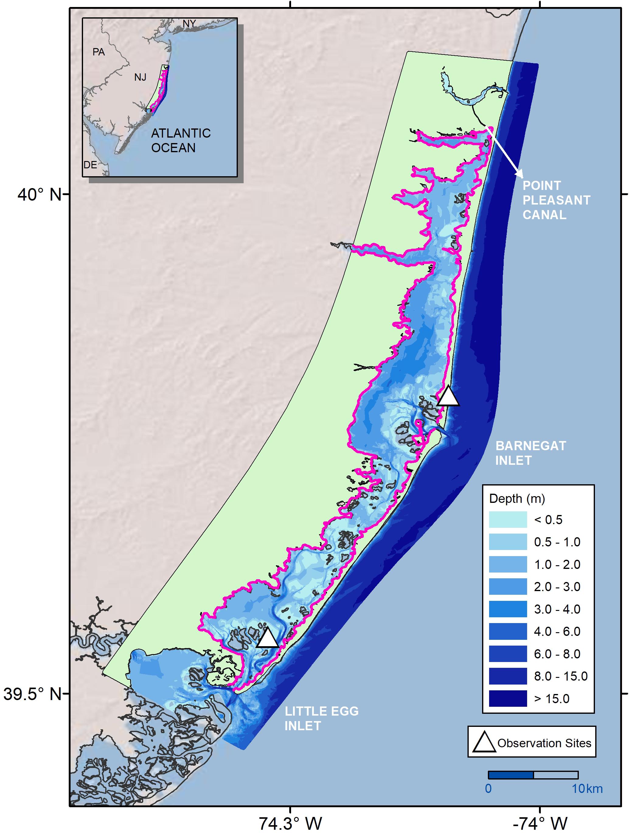
Figure 1. Bathymetry of Barnegat Bay-Little Egg Harbor (BB-LEH) estuary and observation sites used to develop the biomass production model in Straub et al. (2015), with Black outline showing the original computational domain of hydrodynamic model, and Pink outline marking the domain of the coupled production-hydrodynamic model.

Over the past 30 years, there has been a documented decrease in seagrass habitat extent and density in BB-LEH (Lathrop and Haag, 2011; Kennish et al., 2013). Prior work has attributed the decrease in seagrass coverage to increased nutrient loading and eutrophication from the rapid development within the Barnegat Bay watershed (Lathrop and Conway, 2001). The estuary is considered highly eutrophic (Bricker et al., 2007), with nutrient loadings highest in the northern, more developed part of the estuary (Pang et al., 2017). Frequent dredging and extensive shoreline hardening are also stressors on the ecosystem (Kennish, 2001). By 1999, 45% of the total shoreline length had been bulkheaded, and 70% of the upland shores were developed (Lathrop and Bognar, 2001). In recent years, R. maritima has begun to colonize seagrass beds in the central bay, mixing in with Z. marina as the density of Z. marina decreases (Barnegat Bay Partnership, 2016).

Analysis Overview

Our spatially explicit modeling approach began with a simplified version of a biomass production model developed for Z. marina growth in BB-LEH by Straub et al. (2015). The biomass production model calculated daily aboveground and belowground biomass at specific locations when provided with water depth, ambient water temperature, photosynthetically active radiation, and nitrogen availability. To establish the spatial patterns of seagrass production in BB-LEH, we executed the biomass production model at each computational grid cell of a hydrodynamic model that was previously configured for the BB-LEH system by Defne and Ganju (2015, 2018) using the Coupled-Ocean-Atmosphere-Wave-Sediment Transport (COAWST) modeling system. The coupled production-hydrodynamic model was run for 1 year (May 1, 2012 to April 30, 2013) using environmental forcing functions from the hydrodynamic model run, the atmospheric model used to force the hydrodynamic model (North American Regional Reanalysis [NCEP NARR] model), and observational data (Straub et al., 2015). We defined a metric to identify suitable habitat, and calibrated the coupled model by adjusting parameters to optimize habitat agreement with recently published areal maps of seagrass extent (Lathrop and Haag, 2011), and to reflect in situ observational data for seagrass biomass (Kennish et al., 2013) while maintaining biomass growth patterns similar to observed trends (Kennish et al., 2008; Straub et al., 2015). We then modified air temperature and water depth by discrete increments to reflect projected changes due to climate change for the region (Collins et al., 2013; IPCC, 2013), and quantified the separate and combined effects on habitat suitability and estuary-wide productivity. Because the land surrounding BB-LEH is highly developed, we maintained the model domain boundaries as sea level increased with the assumption that the managed landforms and slow-eroding salt marshes (<1 m/yr; Leonardi et al., 2016) surrounding the bay will not significantly change total areal habitat availability. Coupled production-hydrodynamic model runs and data analysis were performed using MATLAB version R2018b.

Biomass Production Model

The fundamental equations for the biomass production model were originally formulated by Madden and Kemp (1996) to predict seagrass biomass using a series of theoretically and empirically derived mechanistic equations relating seagrass growth state variables (e.g., above and belowground biomass) to environmental conditions. The Madden and Kemp (1996) seagrass model included species interactions with epiphytes, phytoplankton, and grazers. Buzzelli et al. (1999) and Cerco and Moore (2001) further adjusted and validated the Madden and Kemp (1996) model, and all three models informed the modifications made by Jarvis et al. (2014), who included sexual reproduction in their calculations of Z. marina growth in Chesapeake Bay. The Straub et al. (2015) biomass production model specified to BB-LEH used in the present study was adapted from the Jarvis et al. (2014) model. In our spatially explicit adaptation of the Straub et al. (2015) model, we simplified the model by removing sexual reproduction, as excluding sexual reproduction does not significantly affect model performance for single-year model runs (Jarvis et al., 2014). We also removed species interactions to isolate the effects of SLR and temperature increases on seagrass alone (Table 1).

TABLE 1

Table 1. Equations defining processes within the biomass production model, where t is the model day, dt is the daily timestep, Tw is water temperature (°C).

The biomass production model solved for two state variables, plant aboveground biomass (i.e., shoots, leaves, stems, and flowers) and plant belowground biomass (i.e., roots and rhizomes) with two ordinary differential equations. Aboveground biomass (AGB; Eq. 1) and belowground biomass (BGB; Eq. 2) were computed at a 24-h time step by determining the biomass gained through primary production, and the biomass lost through respiration, two-way translocation of biomass between AGB and BGB, and losses to mortality:

$\begin{array}{c}AGB\left(t\right)=AGB\left(t-\mathit{dt}\right)\hfill \\ +\left(\mathit{PP}+\mathit{BGAG}-\mathit{AGBG}-{\mathit{AR}}_{\mathit{AG}}-\mathit{AGM}\right)\left(\mathit{dt}\right)\hfill \end{array}(1)$

$\begin{array}{c}BGB\left(t\right)=BGB\left(t-\mathit{dt}\right)\hfill \\ +\left(\mathit{AGBG}-\mathit{BGAG}-{\mathit{AR}}_{\mathit{BG}}-\mathit{BGM}\right)\left(\mathit{dt}\right)\hfill \end{array}(2)$

where t is the model day, dt is the daily timestep, PP is primary production, BGAG is upward translocation, AGBG is downward translocation, AR_AG and AR_BG are above and belowground respiration respectively, and AGM and BGM are above and belowground mortality respectively. The biomass production model was environmentally forced by daily time series of photosynthetically active radiation at the water surface (PARs), ambient water temperature (T_w), and dissolved inorganic nitrogen (DIN) in the water-column (N_wc) and sediment (N_sed). The biomass production model was initiated with a set amount of biomass on May 1 (AGB₀ and BGB₀) and run for 1 year.

PP (Eq. 3) was calculated as the product of a temperature-dependent maximum productivity rate (Pmax; Eq. 4), the amount of AGB present at a given time [AGB (t – dt)], photo period (PhotoPD; Table 1, Eq. 5) and a limiting factor of either light (LLIM) or nitrogen availability (NLIM). Pmax was empirically determined under light-saturated conditions by Evans et al. (1986), and adapted for the biomass production model by Jarvis et al. (2014).

$PP=AGB\left(t-\mathit{dt}\right)\times PhotoPD\times Pmax\times MIN[\mathit{LLIM},\mathit{NLIM}](3)$

$Pmax=0.0948+0.0309\times e^{\left(-0.5\times {\left(\frac{T_w-T_{\mathit{opt}}}{3.2964}\right)}^2\right)}(4)$

LLIM was computed from a photosynthesis-irradiance curve (Table 1, Eq. 6) using PAR at depth (PARd; Table 1, Eq. 7), which was calculated from the exponential decay of the PAR at surface (PARs) with increasing depth, scaled by a light-attenuation constant (kd) and accounting for the water surface reflectance (sr). The value of kd was set to 1.9 m^–1, based on empirically determined values observed in seagrass beds in BB-LEH (Ganju et al., 2014) and the average kd calculated for the two sites observed by Straub et al. (2015; Figure 1). Turbidity, dissolved organic matter, and chlorophyll α concentrations were included in the calculation of kd (Ganju et al., 2014). The nitrogen-limitation factor (NLIM; Table 1, Eq. 8) was influenced by the amount of total DIN in the water column (N_wc) and sediment (N_sed) by a ratio of half-saturation constants (K; Table 1, Eq. 9).

AGBG contributed a constant proportion of PP from the AGB pool to the BGB pool (Table 1, Eq. 10). In the Straub et al. (2015) model, upward translocation was a component of the sexual reproduction model, representing seedling growth. Because we did not explicitly include sexual reproduction, we calculated BGAG as a constant fraction of BGB, which was initiated only when Tw exceeded a minimum temperature required for growth (T_crit) and AGB was less than 0.44 g C m^–2 (Table 1, Eq. 11).

AR_AG (Table 1, Eq. 12) and AR_BG (Table 1, Eq. 13) were both temperature-dependent functions, where AR_AG was calculated as a proportion of PP, and AR_BG was calculated as a proportion of the amount of BGB present at a given time [BGB (t – dt)].

Aboveground mortality (AGM; Table 1, Eq. 14) and belowground morality (BGM; Table 1, Eq. 15) were calculated as constant proportions of AGB and BGB, respectively. The aboveground mortality constant (kmAG) and belowground mortality constant (kmBG) had low values for the January 1 to June 14 time period, and higher values from June 15 to December 31. The increase in mortality as a step function was implemented in Straub et al. (2015) to structure the biomass growth curve and simulate the increased mortality in the summer due to heat stress and senescence in the fall. The January-June mortality constants (kmAG₁ and kmBG₁) were determined by model calibration, whereas the June-December mortality constants (kmAG₂ and kmBG₂) were taken from Straub et al. (2015) to maintain the structure of the growth curve.

All parameter values for the biomass production model are listed in Table 2.

TABLE 2

Table 2. Biomass production model parameters and values for the biomass production model.

Coupled Production-Hydrodynamic Model

Defne and Ganju (2015, 2018) configured and assessed a three-dimensional hydrodynamic model for BB-LEH using the COAWST modeling system to analyze residence time and flushing. The hydrodynamic model consisted of 160 east-west and 800 north-south computational grid cells ranging between 40 and 200 m horizontally, seven equidistant vertical layers, and recent bathymetry (Defne and Ganju, 2015, 2018). Defne and Ganju (2015) ran the hydrodynamic model from March 1 through October 10, 2012, forced at the ocean-atmosphere boundary by state variables from the NCEP NARR model using a bulk flux parameterization. Output from this 6-month model run was used in the present study, and the hydrodynamic model was not re-run under climate change scenarios.

The biomass production model evaluated above and belowground biomass at each horizontal grid cell of the hydrodynamic model domain using depth defined by the model bathymetry, excluding areas of the computational domain outside of BB-LEH boundaries (Figure 1). The horizontal domain, depth, and water temperature were the only components of the hydrodynamic model that were integrated with the biomass production model, resulting in a one-way coupled production-hydrodynamic model with no feedback (Defne and Ganju, 2015; Ganju et al., 2016). We confined model computations to grid cells with a depth greater than 0.1 m, because 0.1 m depth is too shallow for seagrass to be fully submerged across the bay given the tidal range (Defne and Ganju, 2015). Areas with depth less than 0.1 m were inundated under the SLR scenarios, but areas outside the current BB-LEH boundaries were not (see section “Air Temperature and SLR Scenarios”).

The coupled production-hydrodynamic model was run from May 1, 2012, to April 30, 2013 to produce spatial patterns of aboveground and belowground biomass for an annual growth cycle. All grid cells were initiated with the same amount of biomass, AGB₀ and BGB₀, to allow seagrass the opportunity to grow in all locations. We then defined suitable seagrass habitat as present or absent in each model grid cell, where suitable habitat was present if both AGB and BGB exceeded the model-initiated biomass (i.e., AGB₀ and BGB₀) at any point over the modeled year.

Spatial Environmental Forcings

The coupled production-hydrodynamic model required forcing by daily water temperature that adequately represented incremental changes in air temperature due to climate change, with minimal computational expense. Thus, to define water temperature as a function of air temperature spatially, linear models were fit between water temperature from the bottom vertical layer of the Defne and Ganju (2015, 2018) hydrodynamic model run with air temperature from the NCEP NARR atmospheric forcing at each horizontal grid cell (further explained in section “Air Temperature Proxy for Water Temperature”).

Air temperature and short-wave radiation (later converted to photosynthetically active radiation) for the coupled production-hydrodynamic model domain were derived from the NCEP NARR model, which had a spatial resolution of four east-west and six north-south model cells over the entire BB-LEH domain.

For the DIN in the water column and sediment forcings, we used the average monthly concentrations across both sites which were monitored to create the nitrogen forcing for the Straub et al. (2015) model (Figure 1). We interpolated a daily time series from the monthly averages and applied the daily DIN forcings uniformly in space to the coupled production-hydrodynamic model.

Air Temperature Proxy for Water Temperature

While the biomass production model was forced by ambient water temperature, future climate scenarios are typically invoked as changes in air temperature. Therefore, we required a forcing function for ambient water temperature that used air temperature as a proxy. BB-LEH is an extremely shallow estuary with energetic tidal and wind mixing, resulting in a well-mixed vertical profile in all but the deepest central portion of the bay [Wedderburn number (We) less than 1; Supplementary Figure 1]. The well-mixed vertical profile indicated that air temperature was likely to be highly correlated to water temperature throughout the water column and therefore to ambient water temperature experienced by seagrass.

We investigated the use of simple linear regressions to predict water temperature from air temperature in BB-LEH using approximately 15 years of water and air temperature measurements from the Jacques Cousteau National Estuarine Research Reserve. The Jacques Cousteau National Estuarine Research Reserve is adjacent to BB-LEH in Great Bay, New Jersey. Four water quality sampling buoys and one meteorological station recorded temperature observations at 15–30 min intervals from 2002 to 2017 (National Oceanic and Atmospheric Administration [NOAA] and National Estuarine Research Reserve System [NERRS], 2017). We performed four simple linear regressions to correlate water temperature data from each of the sampling buoys to the air temperature measurements. High correlations between air and water temperatures in the observational data supported the assumption that air temperature changes could represent water temperature changes under climate change scenarios (Supplementary Figure 2).

Using this assumption, we created a spatially variable ambient water temperature forcing for the coupled production-hydrodynamic model by performing linear regressions at each grid cell between air temperature from the NCEP NARR atmospheric forcing and water temperature from the bottom vertical layer of the hydrodynamic model (Defne and Ganju, 2015, 2018). Modeled regressions between air and water temperature demonstrated high correlations, with coefficients of determination (R²) averaging 0.92 (Supplementary Figure 3C). The average linear regression slope was 0.9, ranging from 0.77 to 1.03 (Supplementary Figure 3A), with an average temperature offset of 3.2°C (Supplementary Figure 3B). The lowest regression slopes and highest temperature offsets (6.0–10.6°C) occurred at the mouth of Oyster Creek where there is a heated outflow from the Oyster Creek Nuclear Generating Station (Kennish, 2001); this area represented 0.2% of the computational domain. Average root mean square error (RMSE) was 1.8°C, ranging from 1.1 to 2.6°C (Supplementary Figure 3D). The highest correlations and lowest RMSE between air and water temperature occurred in shallow regions of the bay, where seagrass is most likely to be found.

Model Calibration

To select a representative model for both seagrass habitat and production, we calibrated the coupled production-hydrodynamic model by modifying AGB₀, BGB₀, and the January-June mortality rate constants (kmAG₁ and kmBG₁) to balance three model skills: (1) accurate prediction of seagrass habitat distribution, (2) prediction of mean biomass values that aligns with observations, and (3) demonstration of an annual growth cycle comparable to the original Straub et al. (2015) model. We chose to modify these parameters (AGB₀, BGB₀, kmAG₁, and kmBG₁) because they were used for calibration in both Madden and Kemp (1996) and Jarvis et al. (2014). The mortality rate constants were modified within a range published in similar models (0.001–0.015 d^–1 by increments of 0.001 d^–1; Madden and Kemp, 1996; Cerco and Moore, 2001; Jarvis et al., 2014; Straub et al., 2015). AGB₀ and BGB₀ were modified within a biomass range of observed and modeled values for May (4–18 g C m^–2 by increments of 2 g C m^–2; Kennish et al., 2013; Straub et al., 2015).

For the first criterion, modeled habitat distribution was compared to the most recently published seagrass vegetation extent mapping which we converted to a presence/absence habitat map (2009; Lathrop and Haag, 2011). Model skill was assessed by overall accuracy in predicting habitat placement, sensitivity (i.e., the true positive rate), specificity (i.e., the true negative rate), and the true skill statistic (TSS; Allouche et al., 2006). We rejected models that had below 70% overall accuracy and less than 0.70 sensitivity and specificity, and selected models which maximized TSS while also satisfying the other two model selection criteria. The biomass production model parameters were specified to Z. marina, but were used to describe seagrass habitat extent throughout the system because seagrass presence and absence was not differentiated by species in the vegetation mapping.

To align the biomass values within observed ranges for the second criterion, we found ranges in AGB and BGB for the corresponding year (2009) in annual survey data from six transects along a north-south gradient in BB-LEH (Kennish et al., 2013). We converted maximum observed biomass from June-July in dry weight m^–2 (15.1–46.3 g dry wt m^–2 for AGB, and 43.0–103.3 g dry wt m^–2 for BGB) to a range of peak values in g C m^–2 (5–20 g C m^–2 for AGB, and 14–40 g C m^–2 for BGB), accounting for the variability in the percent C in dry weight of Z. marina (30–40%; Duarte, 1990; Fourqurean et al., 2012). Models were selected with peak mean AGB and BGB values in habitat areas within or nearly within the observed ranges.

The original Straub et al. (2015) model was validated at three locations, which all demonstrated significant AGB and BGB growth between May 1 and June 15, a pattern that is confirmed in in situ observations showing repeated peak biomass between June and July (Kennish et al., 2013). To replicate this pattern and satisfy the third calibration criterion, parameter combinations that produced models with mean AGB or BGB that dipped significantly below the model initiated value between May 1 and June 15 were rejected.

Air Temperature and SLR Scenarios

We applied 13 scenarios of increasing air temperature and 13 scenarios of increasing sea level in all possible combinations, creating 169 total cases. Air temperature rise scenarios ranged from +0 to +6.0°C and SLR scenarios ranged from +0 to +1.2 m, invoked as discrete increases to temperature and water depth. We determined the upper limits of air temperature and SLR scenarios from the Eastern North America regional projections in 2100 under the highest greenhouse gas emissions scenario (RCP8.5; Collins et al., 2013, Chapter 12, Figure 13.23; IPCC, 2013, Figures AI.20 and AI.21).

We assessed the impact of the climate scenarios on habitat suitability by calculating percent change in habitat area from the base case scenario of no temperature or SLR. We observed the effects of the climate scenarios on estuary-wide seagrass productivity by looking at integrated total biomass across habitat areas, as well as the mean biomass density in habitat areas over the annual growth cycle. We focused our analyses on temperature scenarios +1.5, +4.0, and +6.0°C, as +1.5°C is the temperature increase identified as a goal for mitigating the effects of climate change, and +4.0 and +6.0°C are close to the temperature increases predicted for Eastern North America under intermediate (RCP4.5) and high (RCP8.5) emissions scenarios (IPCC, 2013). For SLR, we focused on scenarios +0.3, +0.6, and +0.8 m, because +0.6 and +0.8 m are the predicted increases under intermediate (RCP4.5) and high (RCP8.5) emissions scenarios, and +0.3 m is a conservative low-rise scenario (Collins et al., 2013).

Sensitivity Analysis

We tested model sensitivity to changes in biomass production model parameters to achieve two goals. The first goal of the sensitivity analysis was to identify the parameters which had the greatest influence on model predictions to understand where additional parameterization would improve model performance. The second goal was to investigate model behavior to help with our interpretation of the climate change scenario outcomes. For this analysis, we performed model runs with no temperature or SLR modifying 17 biomass production model parameters by ±5 and ±10% from the calibrated model values, and the date of the mortality shift (JDm) by ±5 and ±10 days, while holding all other parameters constant (Table 2). We then calculated the percent change in suitable habitat area and peak mean biomass from the base case for each parameter. For parameters that influence particular state variables, such as PP, LLIM, or NLIM, we also calculated the average percent change in the peak value of that state variable from the base case.

Results

Calibration Results

Our calibrated model set kmAG₁ to 0.003 d^–1 and kmBG₁ to 0.01 d^–1, and AGB₀ and BGB₀ to 12 and 18 g C m^–2, respectively. The model had an overall habitat prediction accuracy of 71.9%, sensitivity of 0.765, specificity of 0.709, and 0.473 TSS (Figure 2). Of the 12 calibration parameter combinations that satisfied our calibration criteria and were within 0.005 of the maximum TSS, the selected parameters were closest to the values used in the Straub et al. (2015) model. Modeled seagrass had a maximum depth of 1.22 m, and a median depth of 0.8 m. Seventy-eight percentage of mapped seagrass occurred in depths less than 1.22 m with a median depth of 0.9 m, and a maximum observed depth of 4.6 m. The greatest deviation between modeled and observed seagrass was the overestimation of habitat presence, or false presence, near Barnegat Inlet and Little Egg Inlet, as well as along the southwestern edge of the bay (Figure 2C). False absence of habitat, where the model omitted habitat in locations with mapped habitat present, occurred primarily at the edges of seagrass meadows that were otherwise accurately represented by the model (Figure 2C). The calibrated model placed habitat in nearly 38% of the model domain, whereas observed seagrass was mapped to cover approximately 19% of the model domain (Figure 2).

FIGURE 2

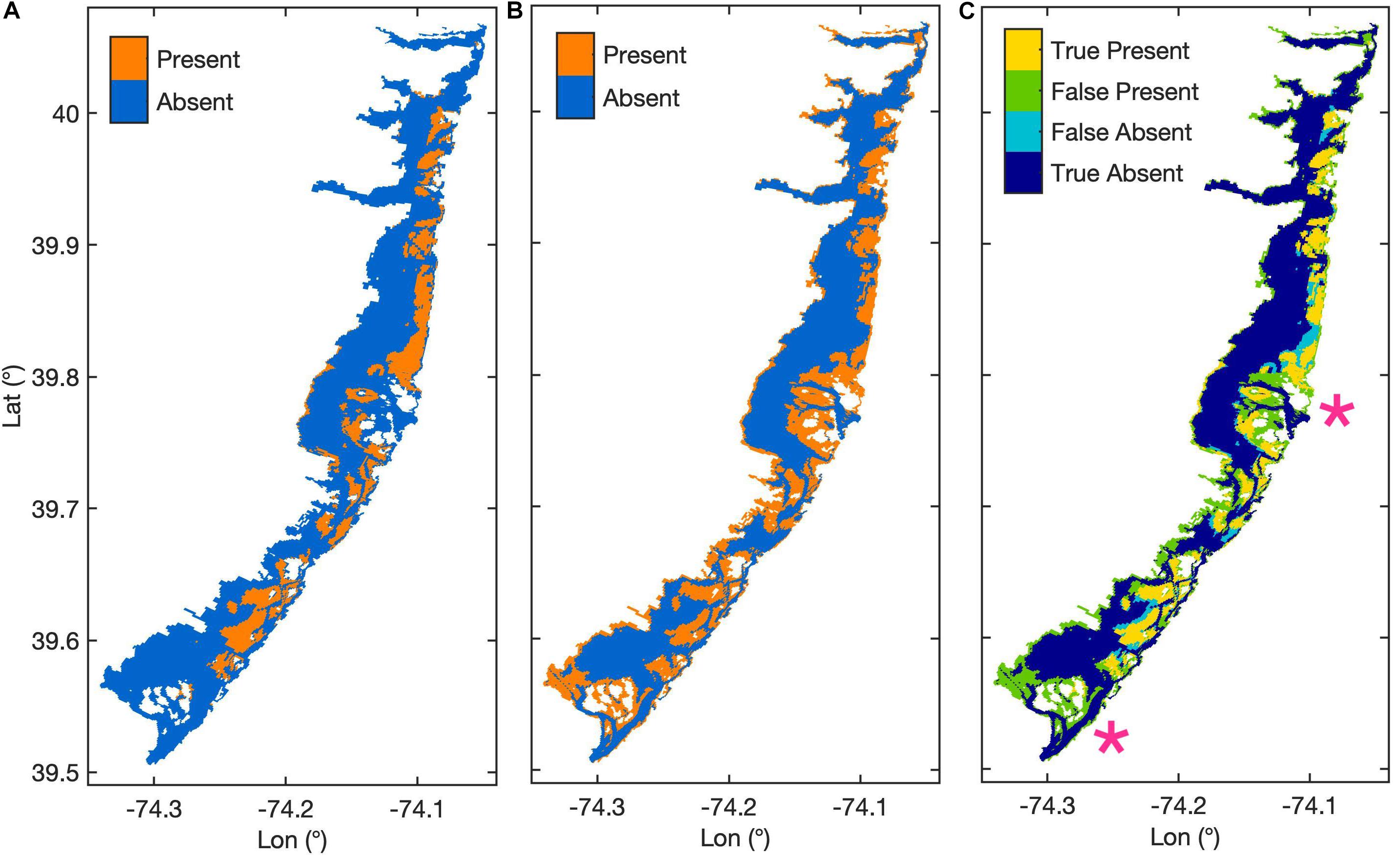
Figure 2. Maps of modeled area where (A) shows mapped seagrass habitat extent in 2009 from Rutgers CRSSA (Lathrop and Haag, 2011), (B) shows the base case modeled seagrass habitat extent, and (C) shows the agreement between the modeled habitat in the base case and mapped habitat extent, with pink stars marking the central and lower inlets.

Within habitat areas, mean AGB peaked at 27.4 g C m^–2, which exceeded the observed maximum AGB in the 2009 in situ survey data (20 g C m^–2), and mean BGB peaked at 22.9 g C m^–2, falling within the observed range of BGB in 2009 (14–40 g C m^–2; Kennish et al., 2013; Figure 3). Biomass growth curves followed those demonstrated in Straub et al. (2015), with AGB growth exceeding BGB growth, and both biomass pools reaching a maximum value on June 15th when higher mortality rates were triggered (Figure 3). Lowering peak AGB to align with observed biomass values depressed model growth of BGB, as BGB growth relied on downward translocation, calculated as a proportion of primary production (see Table 1, Eq. 2). When we could not achieve sufficient BGB growth to simulate realistic growth curves, we decided to increase the allowable AGB growth to exceed observed values up to 30 g C m^–2. While mean BGB growth was modest, the grid cell with maximum BGB growth of the calibrated model demonstrated successful simulation of the biomass growth curve demonstrated in Straub et al. (2015; Figure 3).

FIGURE 3

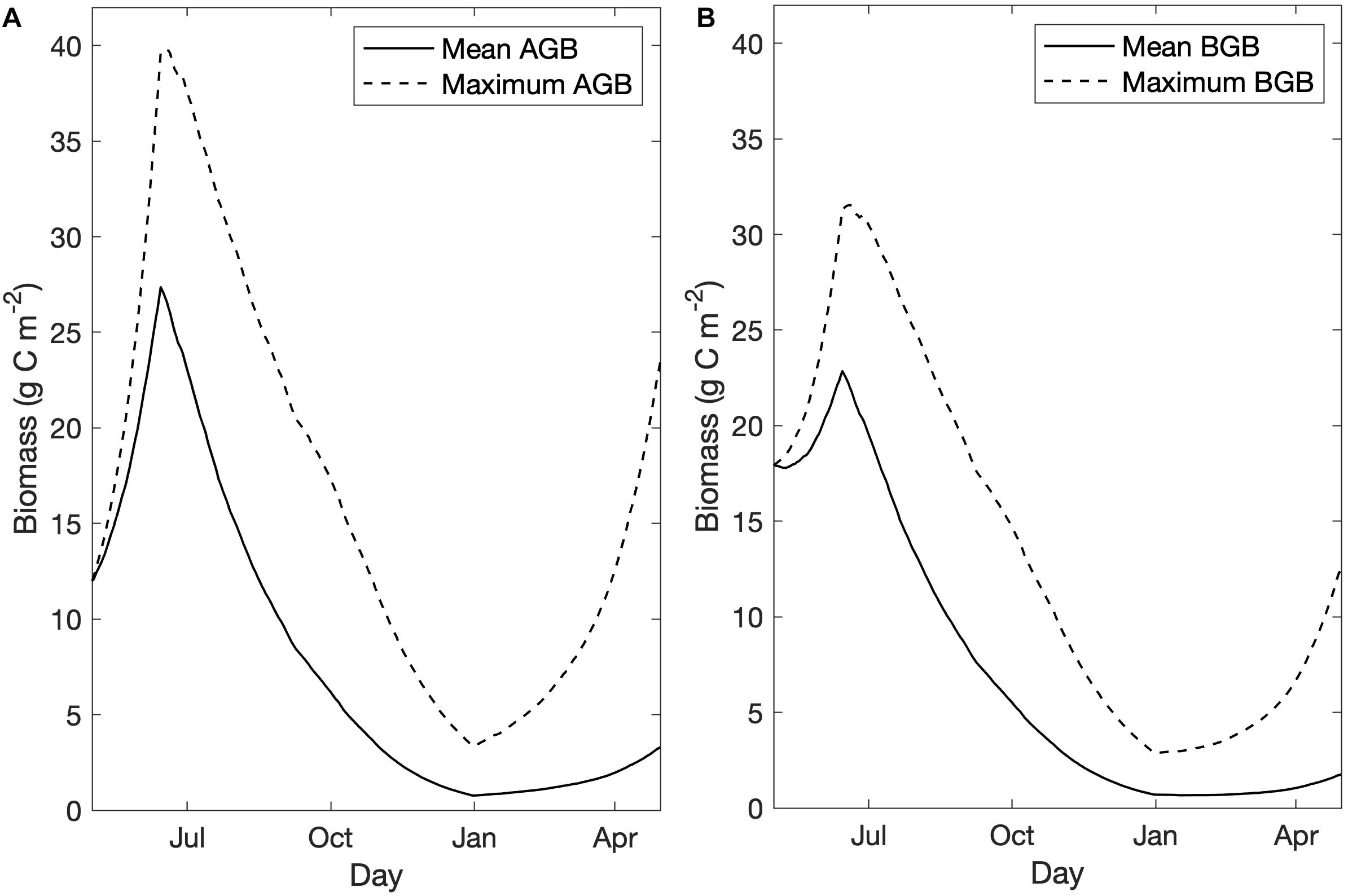
Figure 3. Mean and maximum biomass (g C m^–2) in habitat areas over time for the base case scenario for (A) aboveground biomass, and (B) belowground biomass.

Climate Change Scenario Results

Habitat Suitability

SLR scenarios resulted in a sharp decline in habitat area, with the maximum sea level scenario causing 100% habitat loss for all increasing temperature scenarios (Figure 4). The inverse relationship between SLR and habitat area indicated that depth was a highly deterministic variable in establishing suitable habitat in the model. The effect of SLR on habitat area was not significantly modified by changes in temperature (Figure 4). Temperature rise scenarios +1.5 and +4.0 C had little effect on habitat area, with the former resulting in a 1.4% expansion of habitat area, and the latter causing a 2.5% decrease in habitat area (Figure 4). The highest temperature rise scenario (+6.0 C) produced the greatest decrease in habitat area from temperature alone, with a decline of 8.7% (Figure 4). Decreases in habitat area at higher temperatures were likely caused by both decreased primary production and increased respiration resulting in a higher light compensation point and a shallower depth limit.

FIGURE 4

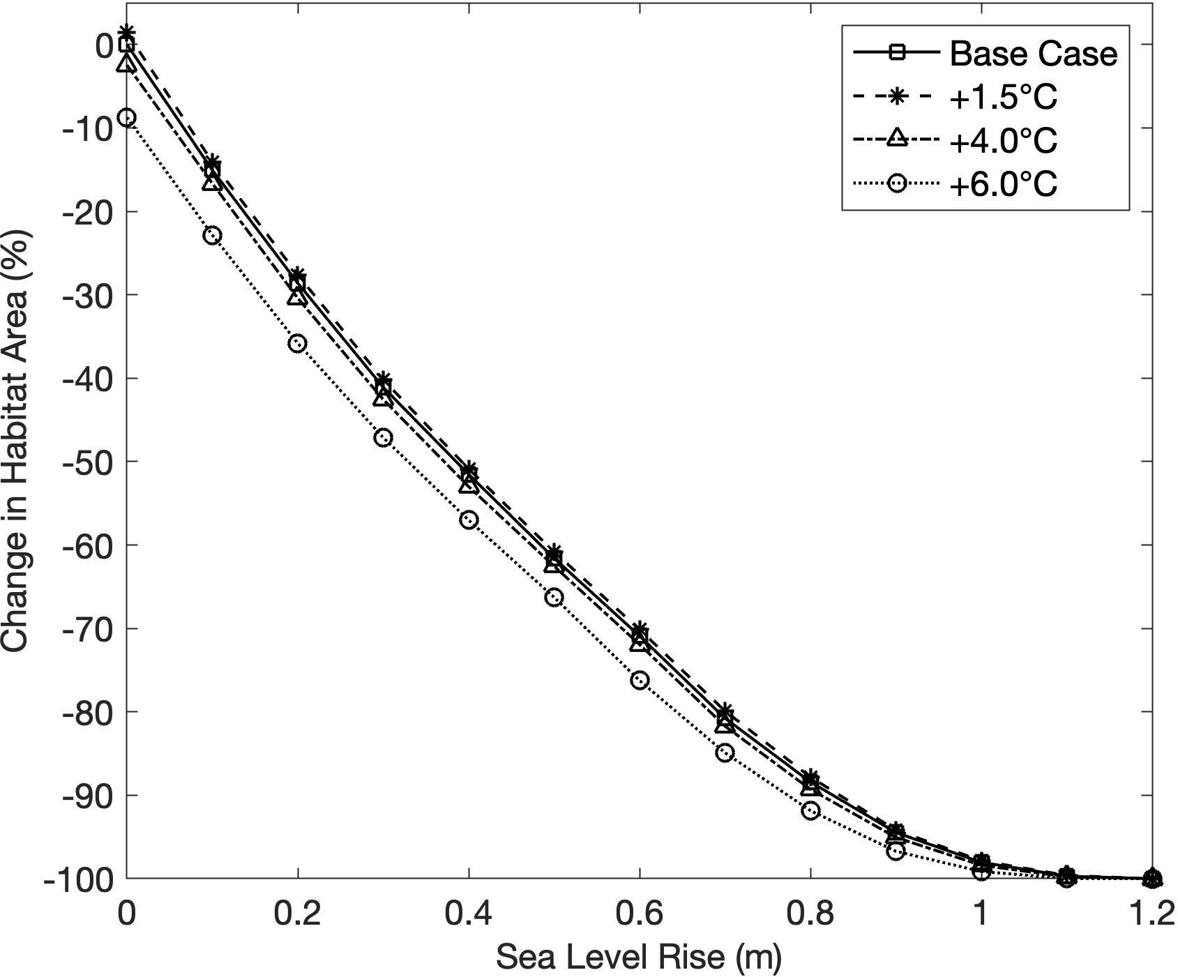
Figure 4. Change in habitat area from the base case scenario for all sea level rise (SLR) scenarios, under four temperature rise scenarios.

Areal maps of habitat area under increasing SLR scenarios show habitat area receding away from the deepening channels, and being squeezed against the barrier islands and coastline (Figure 5). At +0.6 m SLR, over two thirds of the original habitat area was lost, most substantially in the southern third of BB-LEH (Figure 5C). At +0.8 m SLR, there was a near complete loss of seagrass in the north and south ends of the bay, with small beds remaining near Barnegat Inlet (Figure 5D). By the maximum SLR scenario, all suitable habitat disappeared (Figure 5E).

FIGURE 5

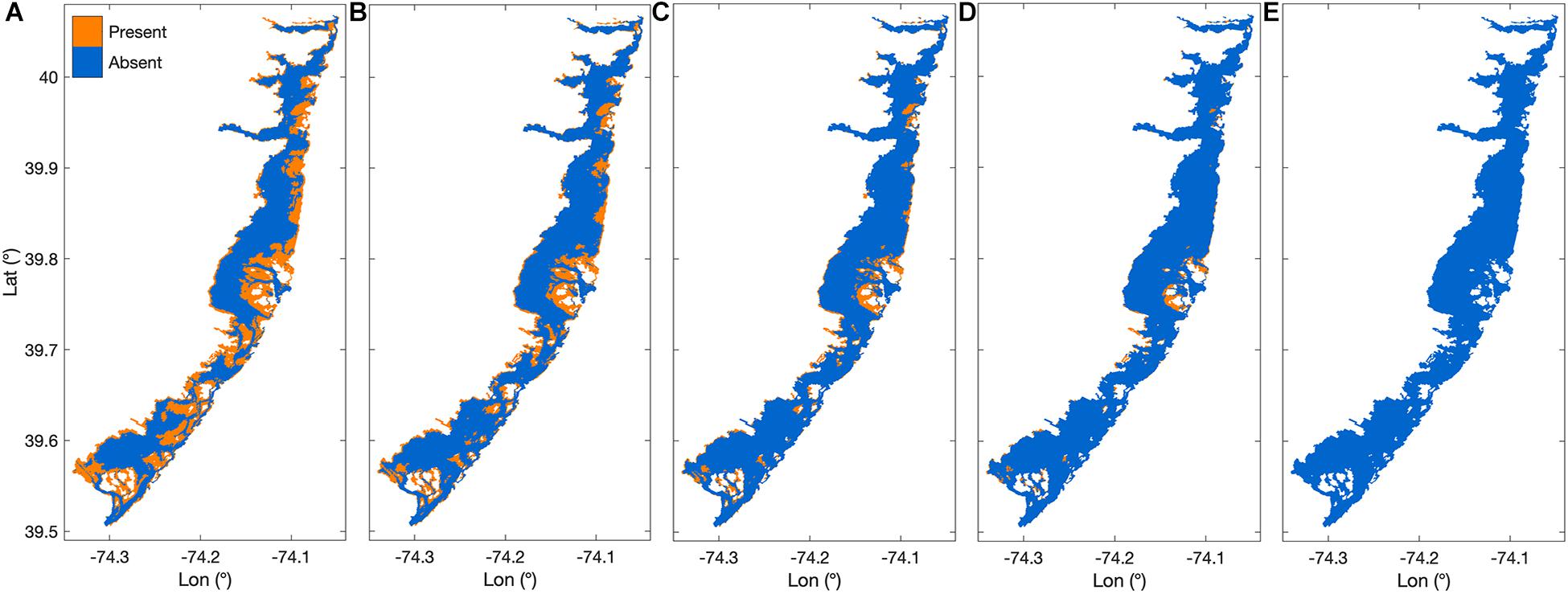
Figure 5. Areal habitat maps showing increasing sea level rise scenarios (SLR) where (A) shows the base case scenario, (B) habitat after +0.3 m SLR, (C) habitat after +0.6 m SLR, (D) habitat after +0.8 m SLR, and (E) habitat after +1.2 m SLR.

Seagrass Productivity

While SLR had a drastic effect on seagrass habitat area, the effect of SLR on seagrass growth in areas that remained suitable habitat was less severe (Figure 6A). Peak mean biomass in habitat areas decreased with increasing SLR scenarios, declining approximately 20% from the base case with +0.8 m SLR (Figure 6A). Seagrass growth was highest at shallow depths, and as depth increased with SLR, originally shallow areas that were still suitable habitat had increased light limitation and slower growth, thus lowering the mean biomass across habitat area. Temperature rise did not strongly affect seagrass productivity in areas with suitable habitat, shown by the minimal effect of temperature rise on seagrass growth rates or peak mean biomass (Figure 6B). Temperature rise did increase the rate of seagrass die-off, likely due to higher losses due to respiration at higher temperatures (Figure 6B).

FIGURE 6

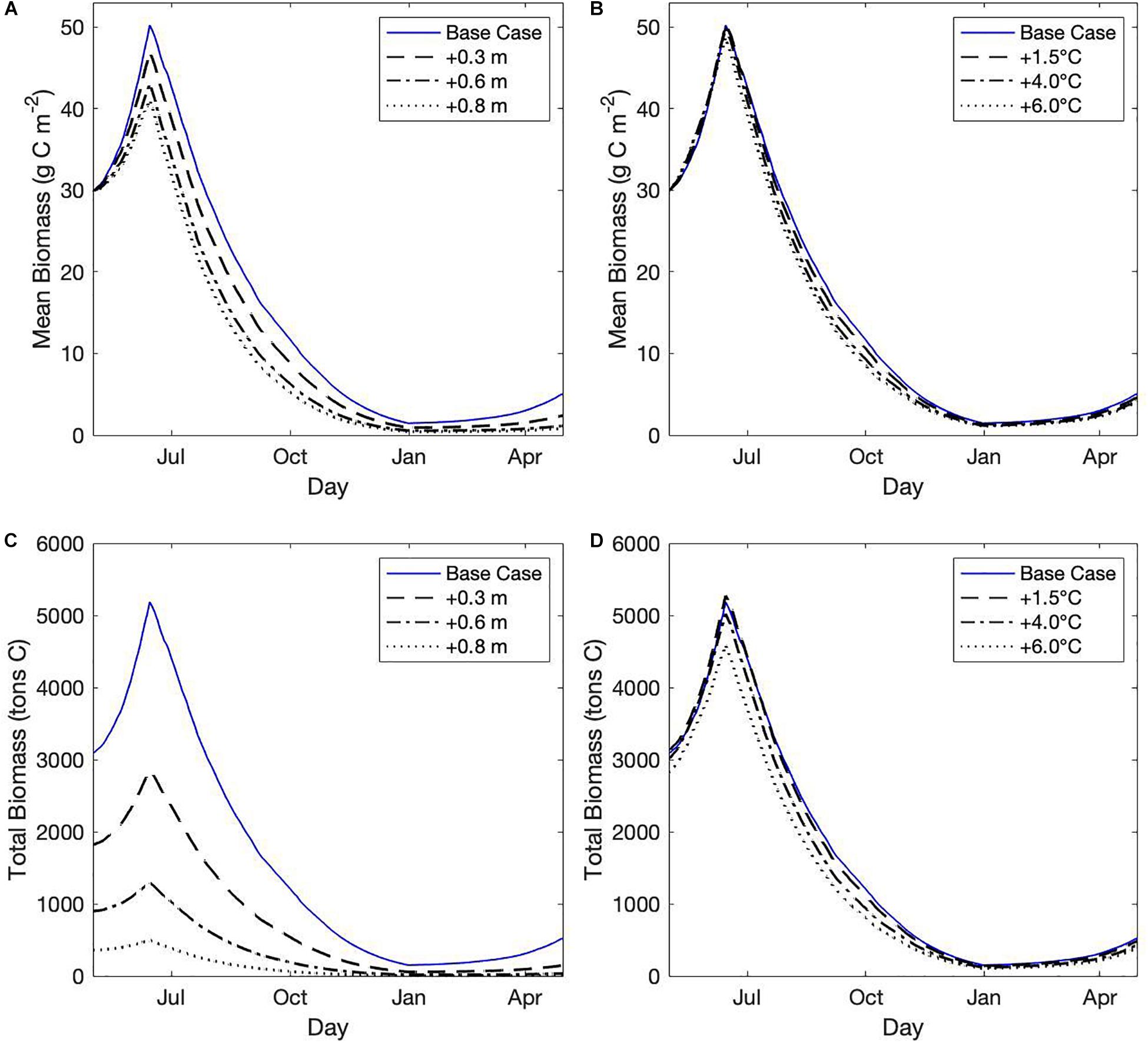
Figure 6. (A,B) Mean cumulative biomass (g C m^–2) in habitat areas over time across (A) select sea level rise (SLR) scenarios, and (B) select temperature rise scenarios. (C,D) Total integrated biomass (tons C) across habitat areas for (C) select SLR scenarios, and (D) select temperature rise scenarios.

Integrated total biomass (tons C) across habitat area, which was a function of both suitable habitat area and seagrass growth, showed that SLR could severely decrease the total carbon storage of the estuary (Figure 6C). Integrated total biomass was only slightly affected by temperature rise due to the effect that temperature increases had to habitat suitability (Figure 6D).

Sensitivity Analysis

Habitat area was most sensitive to changes in kd, kmBG₁, AGB₀, BGB₀, and the date of mortality increase (JDm; Figure 7A). Changes to the half-saturation of light constant (K_i) and the downward translocation constant (Tr_D) also influenced habitat area. Peak mean biomass in habitat areas was similarly most sensitive to changes in JDm, followed by AGB₀, BGB₀, and Tr_D (Figure 7B). Increasing either AGB₀ or BGB₀ resulted in a greater peak mean biomass, but increasing BGB₀ counter intuitively resulted in a decline in habitat area (Figure 7). This dynamic was observed because when BGB₀ was increased while AGB₀ remained constant, the proportion of BGB lost to mortality and respiration exceeded the amount gained by downward translocation, resulting in fewer grid cells where BGB at some point exceeded BGB₀. Habitat area and peak mean biomass were both sensitive to changes in the January–June mortality rates (kmAG₁ and kmBG₁) but were unaffected by changes to the July–December mortality rates (kmAG₂ and kmBG₂). Modifying the higher June-December mortality rates did not have an effect, because habitat area and peak mean biomass were both determined by the first 45 days of growth (May 1 through June 15).

FIGURE 7

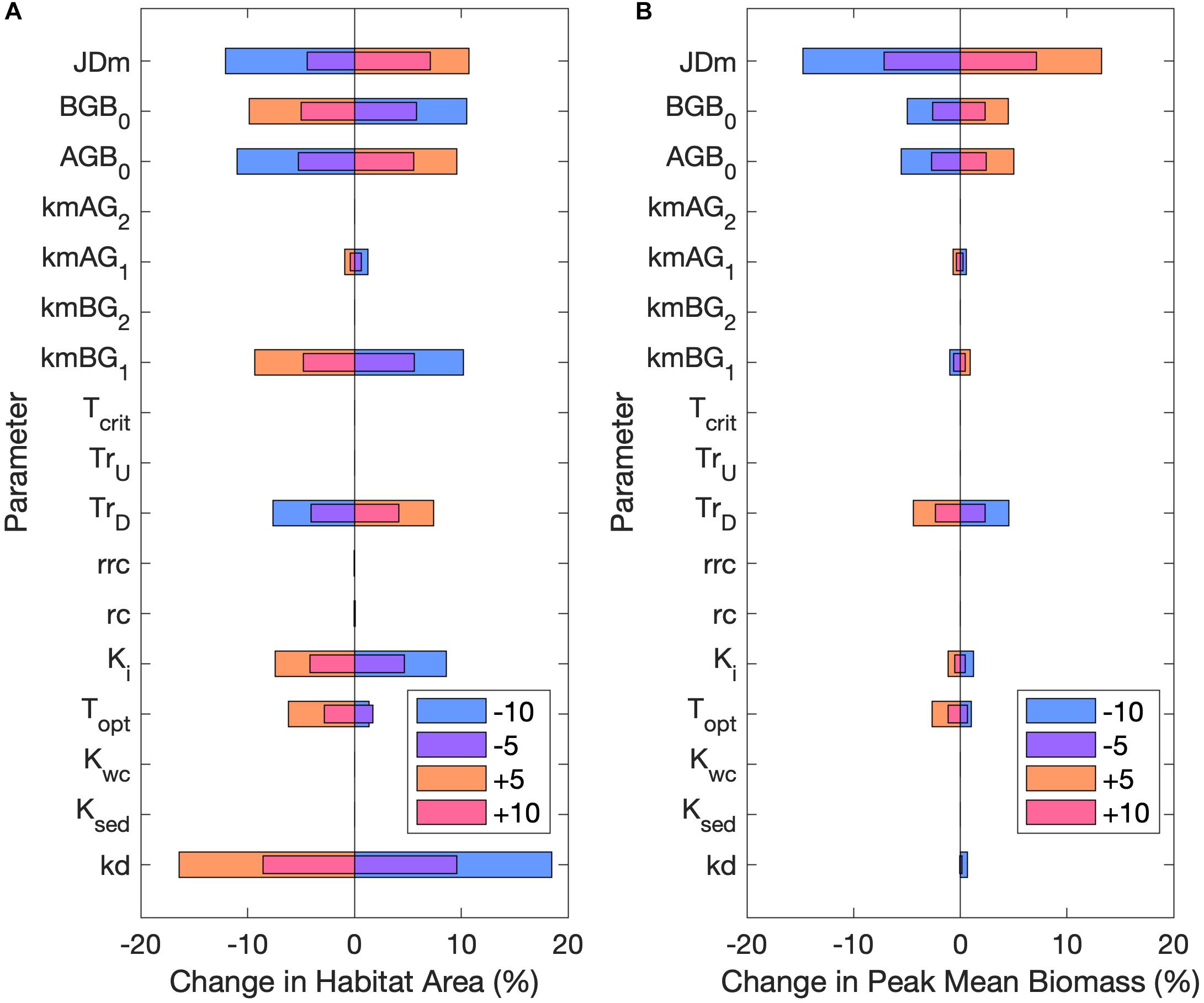
Figure 7. Percent change in (A) habitat area and (B) peak mean biomass from the base case for ±5 and ±10 of all parameters in sensitivity analysis. Legend unit is percent for all parameters expect JDm, which is in days. Refer to Table 2 for parameter definitions.

The optimal temperature for growth (Topt) influenced both habitat area and peak mean biomass, where decreasing Topt resulted in a slight increase in both variables, with the opposite effect occurring for increased Topt. The expansion of habitat with decreased Topt indicated that ambient water temperatures during the important growing season (May–June) of the base case were below the optimal temperature for growth, which helps to explain the habitat expansion under low temperature rise scenarios. Conversely, increasing Topt increased the difference between water temperatures and Topt which led to decreased habitat extent. The high temperature rise scenarios also increased the difference between water temperatures and Topt, thereby similarly resulting in decreased habitat area.

Modifying the upward translocation coefficient (T_U), the critical temperature for germination (T_crit), the DIN half saturation constants in the water column (K_wc) or sediment (K_sed), the root respiration rate at Topt (rc), or the root respiration coefficient (rrc) had little or no effect on habitat area or peak mean biomass.

Primary productivity was strongly influenced by changes in kd, moderately influenced by K_i and Topt, and not influenced by K_wc or K_sed (Supplementary Figure 4A). The light limitation factor (LLIM) was sensitive to change in both kd and K_i (Supplementary Figure 4B), while the peak nutrient limitation factor (NLIM) was minimally affected by changes in K_wc or K_sed (Supplementary Figure 4C).

Discussion

We established a simple, spatially explicit seagrass model that provided a theoretical setting to explore the effects of sea level and temperature rise on estuary-wide seagrass viability. Based on the findings of other modeling studies, we hypothesized that SLR would cause shifts in seagrass habitat distribution following the changes in light attenuation resulting from increased water depth (Saunders et al., 2013; del Barrio et al., 2014; Davis et al., 2016). Previous studies suggested that temperature increases would decrease seagrass growth by decreasing primary productivity and increasing respiration rates (Carr et al., 2012; Jarvis et al., 2014), but the effects of temperature rise on both estuary-wide productivity and habitat area had not previously been explored in the literature. Our climate change simulations indicated that SLR could lead to drastic decreases to suitable habitat extent in BB-LEH, squeezing seagrass beds landward toward the barrier islands. Under the highest emissions scenario, projected SLR resulted in a complete loss of Z. marina in BB-LEH, exceeding the effects of SLR demonstrated for other systems (Saunders et al., 2013; Davis et al., 2016). Contrary to our predictions, temperature rise only slightly increased the rate of summer die-off and had a limited effect on habitat area, with substantial habitat loss observed only under the highest temperature rise scenarios. Our results highlight the importance of creating site specific predictions, as the species composition and regional projections for climate change elevate the vulnerability of the seagrass meadows in BB-LEH to losses due to SLR.

Model Performance

The calibrated model achieved high spatial accuracy in the base case, comparable to other similar modeling studies (55.1–91.5%, Davis et al., 2016; 73.4%, del Barrio et al., 2014), and realized the observed biomass growth curves modeled in the source biomass production model (Straub et al., 2015). In model calibration, along with modifying mortality rate constants and initial biomass values, we increased the light-attenuation constant to 1.9 m^–1, which was slightly above the median value observed (1.7 m^–1, Ganju et al., 2014) to appropriately capture spatial placement along depth gradients. While the model did not predict seagrass to the full observed depth range, the model predicted suitable habitat to 1.22 m which accounts for over 78% of mapped seagrass (Lathrop and Haag, 2011). Previous studies show that the accuracy of seagrass biomass models which rely on the inverse relationship to depth for habitat placement perform highest when separate models are fit to areas with clear or turbid waters (Duarte et al., 2007). Within BB-LEH, high light attenuation results from sediment-induced turbidity (Ganju et al., 2014), and increasing the value of kd helped to reflect the potential impacts of variable turbidity across the bay.

Much of the deviation between the modeled and observed habitat extent occurred from the model overestimating habitat presence in locations where it was not actually observed, most distinctly surrounding the two inlets, Barnegat Inlet and Little Egg Harbor Inlet. While these areas are shallow enough to support seagrass communities, the rapid geomorphic change and high tidal velocities near the inlets could prevent seagrass from colonizing the shoals in these regions (Stevens and Lacy, 2012). Accounting for geomorphic change or current velocity in the model could help improve habitat prediction accuracy (Valle et al., 2014). Including these dynamics in future work would require additional parameterization of the biomass production model to establish the physiological response of seagrass growth to changes in these hydrodynamic variables (Peralta et al., 2006). Alternatively, the areas surrounding the inlets could experience higher light attenuation due to resuspension-induced turbidity which was not explicitly modeled in this analysis. Implementing spatially variable light-attenuation constants that account for turbidity could improve our model predictions (Duarte et al., 2007), particularly because habitat suitability was highly sensitive to changes in kd.

Seagrass Response to Climate Change Scenarios

Increasing sea level resulted in a consistent decline in habitat area, demonstrating the sensitivity of Z. marina distribution to changes in depth. Our model projected that as sea level increased, currently available habitat shifted closer to the barrier islands, following the shifting light attenuation gradient. Under the assumption that SLR will not change the boundaries of available habitat, seagrass habitat was pushed to the estuary boundaries and prevented from establishing new habitat. Saunders et al. (2013) termed this process as “coastal squeeze,” a pattern that has been well-documented in other modeling studies which do not allow for habitat expansion under SLR (Davis et al., 2016; Mills et al., 2016). Other studies that have modeled the effects of increasing light limitation on seagrass habitat have similarly shown that available habitat is primarily determined by light climate. Saunders et al. (2017) simulated that increasing suspended sediment load decreased seagrass habitat availability by increasing light attenuation. Likewise, Cerco and Moore (2001) explored the effects of eutrophication on seagrass distribution and growth, and found that seagrass density spatially followed the same contours as light attenuation, with decreasing density as light attenuation increased.

The modeled habitat loss due to coastal squeeze under SLR was partially due to constraining the model domain to the current boundaries based on the highly developed coastline (Lathrop and Bognar, 2001) and slow erosion rates of surrounding salt marshes (Leonardi et al., 2016). Other studies have demonstrated that if coastal areas are allowed to naturally convert to open water under SLR, marine habitats have the potential to expand in the future (Valle et al., 2014; Mills et al., 2016; Schuerch et al., 2018). Furthermore, in a coastal system without human modification, SLR would cause the barrier islands to shift landward, pushing shallow shoals into previously deep water and allowing seagrass communities to maintain suitable habitat area (Saunders et al., 2013). However, analysis of barrier island rollover in BB-LEH following Hurricane Sandy demonstrated that the highly managed, highly developed barrier islands will likely not be able to shift to sustain available habitat under SLR (Miselis et al., 2016). Even if the surrounding salt marshes were eroded in the future, there is no guarantee that seagrass would be able to colonize the new territory, as eroded marsh sediments do not serve as adequate substrate for Z. marina seeds (Wicks et al., 2009). Alternatively, if we were to assume that SLR would breach the barrier islands without converting to natural habitat, increased connectivity with the Atlantic Ocean would introduce a suite of hydrodynamic changes that have been shown to significantly impact seagrass habitat, such as increased wave exposure, tidal range, and current velocity (Tanaka and Nakaoka, 2004; del Barrio et al., 2014; Saunders et al., 2014; Valle et al., 2014; Defne and Ganju, 2015). Decreased wave sheltering from coral reefs due to SLR resulted in decreased seagrass habitat availability in a tropical coastal system (Saunders et al., 2014), which is a protection currently supplied by the barrier islands in BB-LEH (Defne and Ganju, 2015). Increased tidal range would subject a greater area of seagrass habitat to emergence stress, which also negatively impacts seagrass growth (Tanaka and Nakaoka, 2004; Kim et al., 2013). While these scenarios are possible, the current state of coastline hardening and frequent dredging to maintain current navigable waterways in BB-LEH indicate that it would be highly optimistic to model a future scenario that assumes urban and marsh land will convert to open water unimpeded by anthropogenic intervention (Kennish, 2001; Miselis et al., 2016).

While the landward migration of suitable habitat with SLR was in line with the findings of similar modeling work, the magnitude of habitat loss due to SLR exceeded what other studies have suggested for estuaries in other regions. Our model simulated that 100% of suitable habitat disappeared under the maximum SLR scenario. In contrast, Davis et al. (2016) found a maximum seagrass habitat loss of 44%, and Saunders et al. (2013) reported a 17% loss in seagrass habitat, under their respective maximum SLR scenarios. One reason for this disparity comes from the value used for maximum SLR. Our maximum SLR scenario (+1.2 m) exceeded the scenario used in Davis et al. (+0.75 m; 2016), because we used the projected rise for the Eastern North American coast, whereas Davis et al. (2016) used the global average projection. Saunders et al. (2013) used a comparable magnitude of SLR (+1.1 m), but their study system supported six seagrass species, two of which had greater depth limits than Z. marina (Duarte, 1991). The disparity between our results underscores the need for site specific predictions, as the low species diversity and heightened risk of sea level rise along the Atlantic coast elevate the vulnerability of the seagrass meadows in BB-LEH to losses due to climate change.

The effects of sea level rise far outweighed the effects of temperature rise on seagrass growth and habitat extent for modeled meadows in BB-LEH. Habitat area slightly expanded for low temperature rise scenarios and decreased substantially only at the highest temperature rise scenarios. Increasing temperature had little effect on peak mean biomass and only slightly increased the rate of seagrass loss during summer and fall months. Temperature has been shown to influence seagrass depth limits through the trade-off between respiration rates and primary productivity in low light environments (Lee et al., 2007; Tanaka and Nakaoka, 2007). The sensitivity of habitat area to changes in Topt indicated that the leading contributor to habitat loss at high temperatures in our model was likely decreased primary productivity rather than increased respiration.

Other studies have demonstrated non-linear interactions between temperature and sea level. For example, in Chesapeake Bay, seagrass habitat in shallow regions where light was not limiting was found to be more vulnerable to extreme temperatures (Lefcheck et al., 2017). While seagrass meadows in shallow areas did experience higher temperature increases in our model, reflecting this dynamic, we did not simulate an increased influence of temperature when seagrass habitat was limited to shallow regions under increasing sea level scenarios. The effects of temperature rise on habitat area remained constant with SLR, indicating that high temperature increases could further exacerbate the negative impacts of SLR on habitat area.

While light climate is often found to be the most influential factor affecting seagrass growth (Lee et al., 2007), both experimental and modeling studies support the hypothesis that temperature rise will lower seagrass growth and increase mortality (Marsh et al., 1986; Carr et al., 2012; Repolho et al., 2017). Jarvis et al. (2014) assessed the response of simulated seagrass growth to multiple years of temperature stress, and found that with only a 1°C increase in temperature for 1 year, seagrass were unable to recover. Other studies have shown a similar reduction of productivity due to temperature rise, with dramatic losses of biomass occurring when summer temperatures exceed 30°C (Davis et al., 2016). Using an SDM for Z. marina populations along the Atlantic Coast of North America, Wilson and Lotze (2019) projected a complete extinction of seagrass in BB-LEH with a temperature increase projected under the IPCC’s maximum emissions scenario. However, their model assumed that water temperatures were already limiting in BB-LEH. Straub et al. (2015) have shown that daily mean water temperatures in BB-LEH seagrass meadows ranged between 0 and 28°C with the highest temperatures not lasting more than 5 consecutive days, shorter than the time periods observed to result in Z. marina thermal die-off events (Moore and Jarvis, 2008). Therefore, while temperature rise is a demonstrated threat to Z. marina, our model results suggest that rising sea level presents a more severe threat to BB-LEH. Under our conservative SLR scenario, which increased sea level by less than half of the projected increases under a maximum emissions scenario, habitat area dropped by over 40%, and integrated total biomass fell by nearly half. The Wilson and Lotze (2019) study did not investigate SLR and the associated changes to light availability.

The muted response of habitat area and biomass production to increasing temperature in our model compared to the impacts demonstrated in other studies could be due to insufficient representation of mortality temperature dependence in the biomass production model, and the lack of extreme temperature events in our climate scenarios. Although extreme temperatures have been repeatedly linked to spikes in mortality (Moore and Jarvis, 2008; Smale and Wernberg, 2013), the mathematical relationship between mortality and temperature is not well-established for seagrass in BB-LEH and was therefore not explicitly included in the Straub et al. (2015) model. This was partly compensated in the model by employing two constant mortality rates, with higher mortality from mid-June through the end of the year to simulate increased mortality in summer and leaf sloughing in fall and winter. Using constant mortality rates could have oversimplified the impacts of temperature, leading to the low biomass responses to changes in temperature. Furthermore, the most severe impacts of increased temperatures on seagrass have been demonstrated to occur during marine heat waves (Moore and Jarvis, 2008; Moore et al., 2012; Smale and Wernberg, 2013), which are expected to increase in frequency and duration with increased global temperatures (Oliver et al., 2018). Our temperature scenarios represented increases in mean air temperature expected with climate change, and did not simulate increased variability in temperature extremes.

Based on the sensitivity analysis, mortality parameters, such as the date on which high summer-fall mortality was triggered in the model and the January–June mortality rates, were highly influential on model results, highlighting the importance of accurately parameterizing mortality. Habitat area and peak mean biomass were only sensitive to parameters that impact the first 45 days of growth, i.e., the time period before high mortality was triggered. Previous studies have demonstrated that seagrass population viability relies on successful spring-time growth (Moore et al., 1997), which aligns with our model’s reliance on late spring growth to define successful habitat. While the date of mortality increase was determined to match present-day conditions, increases to year-round temperatures could shift summer mortality to earlier in the year, which was not reflected in our temperature rise scenarios (Clausen et al., 2014).

Model Limitations and Caveats

An important goal of this study was to provide a simple system approach to efficiently test the sensitivity of seagrass to changes in sea level and temperature, and thus we did not aim to capture every biogeochemical and hydrodynamic process that impacts seagrass meadows. However, the exclusion of other processes limits the extent to which our model can fully capture responses to future changes in physical conditions. One such limitation was the exclusion of epiphytes and phytoplankton, which can be important controls on light climate, and respond to changes in temperature and nutrient availability (Cerco and Moore, 2001; Thomsen et al., 2012; del Barrio et al., 2014). Because we isolated the impacts of water depth and temperature on seagrass, and did not modify nutrients, we did not simulate changes in nutrient-sensitive epiphytes and phytoplankton. Their effects were, however, included in the model implicitly, as epiphytes and phytoplankton factor into present day habitat distribution and growth for which the model was calibrated. Furthermore, the empirical evaluation of kd in BB-LEH by Ganju et al. (2014) included the effects of phytoplankton on light attenuation. If epiphytes and phytoplankton were to be modeled explicitly, more sophisticated nutrient dynamics would need to be employed in the model to capture spatial patterns in eutrophication (del Barrio et al., 2014; Ganju et al., 2014).

Because the hydrodynamic model was not re-run under the climate change scenarios, we did not simulate any bathymetric changes that could occur due to increased erosion and accretion under SLR. While shoal accretion could contribute to seagrass habitat redistribution or expansion (Barillé et al., 2010), changes to bathymetry in BB-LEH under SLR may be limited by the current shoreline hardening and dredging practices (Kennish, 2001; Miselis et al., 2016). Hydrodynamic feedbacks that occur with the loss of seagrass meadows were also not represented in the model, such as increased wave action and sediment resuspension, which could have amplified the negative impacts of future change on seagrass habitat by contributing to elevated light attenuation (Saunders et al., 2014; Carr et al., 2016; Saunders et al., 2017). By excluding these negative feedbacks, our model results present a best case scenario for seagrass under future climate change scenarios.

In our climate change scenarios, we implemented discrete increases in temperature and sea level on a single year of growth, which allowed us to assess their separate and combined impacts on seagrass in BB-LEH. More realistic climate change scenarios, however, would have a continuous increase in temperature and sea level over time, with an accumulation of stress over multiple years and potential adaptation of the seagrasses to this stress. The most dramatic effects of temperature rise on seagrass have been shown with multiple years of temperature stress, which we did not include in our simulations (Jarvis et al., 2014; Davis et al., 2016). We were confined to 1-year model runs because we only accounted for the biomass gains through productivity, and not sexual reproduction. While ignoring sexual reproduction is a validated method for modeling seagrass, Jarvis et al. (2014) concluded that model runs longer than 1 year are significantly less accurate when sexual reproduction is ignored. If the model were to be run for longer than 1 year, sexual reproduction would likely need to be incorporated, including the potential for horizontal movement of seagrass through colonization. Future iterations of the model which may include dispersal of sexual reproductive propagules could allow for recolonization of grid cells that have lost all biomass. For significantly longer model runs, the model would be improved by incorporating the potential for local adaptation of seagrass to environmental change, as Z. marina demonstrates appreciable plasticity through regional adaptations to different light and temperature climates (Short et al., 2007; Wilson and Lotze, 2019).

The model was further limited by not explicitly including the other seagrass species found in BB-LEH, Ruppia maritima. R. maritima is a more environmentally tolerant species than Z. marina, which could allow for R. maritima to colonize habitat that is no longer suitable for Z. marina (Wetzel and Penhale, 1983; Evans et al., 1986; Short et al., 2007; Moore et al., 2014).

Finally, our study focused solely on the projected increases in sea level and temperature due to climate change, and did not account for other factors which may alter the future environment of BB-LEH. Future increases in atmospheric CO₂ depositing into the ocean will increase available dissolved inorganic carbon for seagrasses. CO₂ enrichment has been shown to accelerate growth and increase reproductive output in seagrasses (Palacios and Zimmerman, 2007), although developing research in this area suggests that the negative effects of temperature will be more significant than any benefit to growth from increased CO₂ (Repolho et al., 2017). Alternatively, conservation strategies could influence a future decrease in nutrient loading, which would have the effect of decreasing phytoplankton abundance, thereby improving the light climate and expanding seagrass habitat (del Barrio et al., 2014).

Conclusion

The simplified seagrass biomass production model, coupled with a spatially explicit hydrodynamic model, provided a theoretical framework to assess the influences of climate change on seagrass viability in Barnegat Bay-Little Egg Harbor (BB-LEH). Under future climate conditions, seagrass habitat and productivity are threatened greatly by projected increases in sea level. Assuming that the extensive shoreline hardening currently in place will not be removed, increasing sea level squeezed seagrass habitat toward the shoreline without room for habitat expansion, leading to a complete loss of seagrass under the maximum sea level rise scenario. While Z. marina habitat and productivity will be impacted by changes in temperature, the negative impacts of sea level rise (SLR) and the resulting reduction in light availability far outweigh the impacts of temperature. Loss of seagrass due to accelerating SLR will likely pose a significant risk to the overall health of the BB-LEH estuary and should be a prominent concern when developing conservation strategies to protect the ecosystem in the future. The risks posed by climate change to BB-LEH due to the low species diversity and higher-than-average SLR may be shared by other similar estuaries along the North American Atlantic Coast (Short et al., 2007; Sallenger et al., 2012). As such, seagrass meadows in other estuaries in the region may be equally as vulnerable to increases in sea level as BB-LEH.

Data Availability Statement

The datasets and model code generated for this study that are not cited in the references can be found in the corresponding author’s GitHub repository, BBLEH-Seagrass-Model. Persistent link: http://doi.org/10.5281/zenodo.3691971.

Author Contributions

JV, JJ, NG, and CS conceived and designed the study. CS, NG, and JJ acquired the data. JJ, JT, NG, and CS formulated the model. CS and NG calibrated the model, analyzed the model output, and conducted sensitivity analyses. CS, NG, JJ, JT, and JV wrote and edited the manuscript. All authors contributed to the article and approved the submitted version.

Funding

This research was supported by the National Science Foundation Research Experience for Undergraduates Program (OCE-1659463), the Woods Hole Oceanographic Institution Summer Student Fellowship Program, the Barnegat Bay Partnership (through a US EPA Clean Water Act grant to Ocean County College; CE98212313), and the USGS Coastal and Marine Hazards/Resources Program. Although this project has been funded in part by the United States Environmental Protection Agency pursuant to a grant agreement with Ocean County College, it has not gone through the Agency’s publications review process and may not necessarily reflect the views of the Agency; therefore, no official endorsement should be assumed. Any use of trade, firm, or product names is for descriptive purposes only and does not imply endorsement by the U.S. Government.

Conflict of Interest

The authors declare that the research was conducted in the absence of any commercial or financial relationships that could be construed as a potential conflict of interest.

Acknowledgments

We would like to thank Zafer Defne for his advice and assistance in the integration of the hydrodynamic model, and for feedback on the manuscript. Further thanks to Alfredo Aretxabaleta for assistance in the mixing model, and Diane Thomson for early guidance on the manuscript. This is UMCES publication number 5911, reference number [UMCES] CBL 2021-014.

Supplementary Material

The Supplementary Material for this article can be found online at: https://www.frontiersin.org/articles/10.3389/fmars.2020.539946/full#supplementary-material

References

Allouche, O., Tsoar, A., and Kadmon, R. (2006). Assessing the accuracy of species distribution models: prevalence, kappa and the true skill statistic (TSS). J. Appl. Ecol. 43, 1223–1232. doi: 10.1111/j.1365-2664.2006.01214.x

CrossRef Full Text | Google Scholar

Aoki, L. R., McGlathery, K. J., Wiberg, P. L., and Al-Haj, A. (2020). Depth affects seagrass restoration success and resilience to marine heat wave disturbance. Estuaries Coast. 43, 316–328. doi: 10.1007/s12237-019-00685-0

CrossRef Full Text | Google Scholar

Baird, M. E., Adams, M. P., Babcock, R. C., Oubelkheir, K., Mongin, M., Wild-Allen, K. A., et al. (2016). A biophysical representation of seagrass growth for application in a complex shallow-water biogeochemical model. Ecol. Modell. 325, 13–27. doi: 10.1016/j.ecolmodel.2015.12.011

CrossRef Full Text | Google Scholar

Barillé, L., Robin, M., Harin, N., Bargain, A., and Launeau, P. (2010). Increase in seagrass distribution at Bourgneuf Bay (France) detected by spatial remote sensing. Aquat. Bot. 92, 185–194. doi: 10.1016/j.aquabot.2009.11.006

CrossRef Full Text | Google Scholar

Barnegat Bay Partnership (2016). 2016 State of the Bay Report. Available online at: https://www.barnegatbaypartnership.org/wp-content/uploads/2017/08/BBP_State-of-the-Bay-book-2016_forWeb-1.pdf (accessed September, 2019).

Google Scholar

Bos, A. R., Bouma, T. J., de Kort, G. L., and van Katwijk, M. M. (2007). Ecosystem engineering by annual intertidal seagrass beds: sediment accretion and modification. Estuar. Coast. Shelf Sci. 74, 344–348. doi: 10.1016/j.ecss.2007.04.006

CrossRef Full Text | Google Scholar

Bricker, S. B., Longstaff, B., Dennison, W., Jones, A., Boicourt, K., Wicks, C., et al. (2007). Effects of Nutrient Enrichment in the Nation’s Estuaries: A Decade of Change NOAA Coastal Ocean Program Decision Analysis Series No 26. Silver Spring, MD: National Centers for Coastal Ocean Science, 322. doi: 10.1016/j.hal.2008.08.028

CrossRef Full Text | Google Scholar

Buzzelli, C. P., Wetzel, R. L., and Meyers, M. B. (1999). A linked physical and biological framework to assess biogeochemical dynamics in a shallow estuarine ecosystem. Estuar. Coast. Shelf Sci. 49, 829–851. doi: 10.1006/ecss.1999.0556

CrossRef Full Text | Google Scholar

Carr, J. A., D’Odorico, P., McGlathery, K. J., and Wiberg, P. L. (2012). Modeling the effects of climate change on eelgrass stability and resilience: future scenarios and leading indicators of collapse. Mar. Ecol. Prog. Ser. 448, 289–301. doi: 10.3354/meps09556

CrossRef Full Text | Google Scholar

Carr, J. A., D’Odorico, P., McGlathery, K. J., and Wiberg, P. L. (2016). Spatially explicit feedbacks between seagrass meadow structure, sediment and light: habitat suitability for seagrass growth. Adv. Water Resour. 93, 315–325. doi: 10.1016/j.advwatres.2015.09.001

CrossRef Full Text | Google Scholar

Cerco, C. F., and Moore, K. (2001). System-wide submerged aquatic vegetation model for Chesapeake Bay. Estuaries Coast. 24, 522–534. doi: 10.2307/1353254

CrossRef Full Text | Google Scholar

Clausen, K. K., Krause-Jensen, D., Olesen, B., and Marbà, N. (2014). Seasonality of eelgrass biomass across gradients in temperature and latitude. Mar. Ecol. Prog. Ser. 506, 71–85. doi: 10.3354/meps10800

CrossRef Full Text | Google Scholar

Collins, M., Knutti, R., Arblaster, J., Dufresne, J.-L., Fichefet, T., Friedlingstein, P., et al. (2013). “Long-term climate change: projections, commitments and irreversibility,” in Climate Change 2013: The Physical Science Basis. Contribution of Working Group I to the Fifth Assessment Report of the Intergovernmental Panel on Climate Change, eds T. F. Stocker, D. Qin, G.-K. Plattner, M. Tignor, S. K. Allen, J. Boschung, et al. (Cambridge: Cambridge University Press).

Google Scholar

Davis, T. R., Harasti, D., Smith, S. D., and Kelaher, B. P. (2016). Using modelling to predict impacts of sea level rise and increased turbidity on seagrass distributions in estuarine embayments. Estuar. Coast. Shelf Sci. 181, 294–301. doi: 10.1016/j.ecss.2016.09.005

CrossRef Full Text | Google Scholar

DeAngelis, D. L., and Yurek, S. (2017). Spatially explicit modeling in ecology: a review. Ecosystems 20, 284–300. doi: 10.1007/s10021-016-0066-z

CrossRef Full Text | Google Scholar

Defne, Z., and Ganju, N. K. (2015). Quantifying the residence time and flushing characteristics of a shallow, back-barrier estuary: application of hydrodynamic and particle tracking. Estuaries Coast. 38, 1719–1734. doi: 10.1007/s12237-014-9885-3

CrossRef Full Text | Google Scholar

Defne, Z., and Ganju, N. K. (2018). USGS Barnegat Bay Hydrodynamic Model for March to September 2012. Reston, VA: U.S. Geological Survey. doi: 10.5066/F7SB44QS

PubMed Abstract | CrossRef Full Text | Google Scholar

del Barrio, P., Ganju, N. K., Aretxabaleta, A. L., Hayn, M., García, A., and Howarth, R. W. (2014). Modeling future scenarios of light attenuation and potential seagrass success in a eutrophic estuary. Estuar. Coast. Shelf Sci. 149, 13–23. doi: 10.1016/j.ecss.2014.07.005

CrossRef Full Text | Google Scholar

Dennison, W. C. (1987). Effects of light on seagrass photosynthesis, growth and depth distribution. Aquat. Bot. 27, 15–26. doi: 10.1016/0304-3770(87)90083-0

CrossRef Full Text | Google Scholar

Duarte, C. M. (1990). Seagrass nutrient content. Mar. Ecol. Prog. Ser. 67, 201–207. doi: 10.3354/meps067201

CrossRef Full Text | Google Scholar

Duarte, C. M. (1991). Seagrass depth limits. Aquat. Bot. 40, 363–377. doi: 10.1016/0304-3770(91)90081-F

CrossRef Full Text | Google Scholar

Duarte, C. M., Marbà, N., Krause-Jensen, D., and Sánchez-Camacho, M. (2007). Testing the predictive power of seagrass depth limit models. Estuaries Coast. 30:652. doi: 10.1007/BF02841962

CrossRef Full Text | Google Scholar

Evans, A. S., Webb, K. L., and Penhale, P. A. (1986). Photosynthetic temperature acclimation in two coexisting seagrasses, Zostera marina L. and Ruppia maritima L. Aquat. Bot. 24, 185–197. doi: 10.1016/0304-3770(86)90095-1

CrossRef Full Text | Google Scholar

Fonseca, M. S., and Fisher, J. S. (1986). A comparison of canopy friction and sediment movement between four species of seagrass with reference to their ecology and restoration. Mar. Ecol. Prog. Ser. 29, 15–22. doi: 10.3354/meps029015

CrossRef Full Text | Google Scholar

Fourqurean, J. W., Duarte, C. M., Kennedy, H., Marbà, N., Holmer, M., Mateo, M. A., et al. (2012). Seagrass ecosystems as a globally significant carbon stock. Nat. Geosci. 5, 505–509. doi: 10.1038/ngeo1477

CrossRef Full Text | Google Scholar

Ganju, N. K., Brush, M. J., Rashleigh, B., Aretxabaleta, A. L., del Barrio, P., Grear, J. S., et al. (2016). Progress and challenges in coupled hydrodynamic-ecological estuarine modeling. Estuaries Coast. 39, 311–332. doi: 10.1007/s12237-015-0011-y

PubMed Abstract | CrossRef Full Text | Google Scholar

Ganju, N. K., Miselis, J. L., and Aretxabaleta, A. L. (2014). Physical and biogeochemical controls on light attenuation in a eutrophic, back-barrier estuary. Biogeosciences 11, 7193–7205. doi: 10.5194/bg-11-7193-2014

CrossRef Full Text | Google Scholar

Hughes, A. R., Williams, S. L., Duarte, C. M., Heck, K. L., and Waycott, M. (2009). Associations of concern: declining seagrasses and threatened dependent species. Front. Ecol. Environ. 7, 242–246. doi: 10.1890/080041

CrossRef Full Text | Google Scholar

IPCC (2013). “Annex I: Atlas of Global and Regional Climate Projections,” in The Physical Science Basis. Contribution of Working Group I to the Fifth Assessment Report of the Intergovernmental Panel on Climate Change [Stocker, T.F., D. Qin, G.-K. Plattner, M. Tignor, S.K. Allen, J. Boschung, A. Nauels, Y. Xia, V. Bex and P.M. Midgley (eds.)], eds G. J. van Oldenborgh, M. Collins, J. Arblaster, J. H. Christensen, J. Marotzke, S. B. Power, et al. (Cambridge: Cambridge University Press).

Google Scholar

Jarvis, J. C., Brush, M. J., and Moore, K. A. (2014). Modeling loss and recovery of Zostera marina beds in the Chesapeake Bay: The role of seedlings and seed-bank viability. Aquat. Bot. 113, 32–45. doi: 10.1016/j.aquabot.2013.10.010

CrossRef Full Text | Google Scholar

Kennish, M. J. (2001). Physical description of the Barnegat Bay—Little Egg Harbor estuarine system. J. Coast. Res. SI (32), 13–27.

Google Scholar

Kennish, M. J., Haag, S. M., and Sakowicz, G. P. (2008). Seagrass demographic and spatial habitat characterization in Little Egg Harbor, New Jersey, using fixed transects. J. Coast. Res. 2008, 148–170. doi: 10.2112/SI55-0013.1

CrossRef Full Text | Google Scholar

Kennish, M. J., Fertig, B. M., and Sakowicz, G. P. (2013). In situ Surveys of Seagrass Habitat in the Northern Segment of the Barnegat Bay-Little Egg Harbor Estuary: Eutrophication Assessment. Technical Report prepared for the Barnegat Bay Partnership. Available online at: https://www.barnegatbaypartnership.org/wp-content/uploads/wpallimport/files/2011%20Northern%20seagrass%20survey.pdf (accessed July, 2017).

Google Scholar

Kenov, I. A., Deus, R., Alves, C. N., and Neves, R. (2013). Modelling seagrass biomass and relative nutrient content. J. Coast. Res. 29, 1470–1476. doi: 10.2112/jcoastres-d-13-00047.1

CrossRef Full Text | Google Scholar

Kenworthy, W. J., Wyllie-Echeverria, S., Coles, R. G., Pergent, G., and Pergent-Martini, C. (2007). “Seagrass conservation biology: an interdisciplinary science for protection of the seagrass biome,” in Seagrasses: Biology, Ecology and Conservation, eds A. W. D. Larkum, R. J. Orth, C. M. Duarte (Dordrecht: Springer), 595–623. doi: 10.1007/978-1-4020-2983-7_25

CrossRef Full Text | Google Scholar

Kim, J. B., Lee, W. C., Lee, K. S., and Park, J. I. (2013). Growth dynamics of eelgrass, Zostera marina, in the intertidal zone of Seomjin Estuary, Korea. Ocean Sci. J. 48, 239–250. doi: 10.1007/s12601-013-0021-2

CrossRef Full Text | Google Scholar

Lathrop, R. G., and Bognar, J. A. (2001). Habitat Loss and Alteration in the Barnegat Bay Region, Journal of Coastal Research. SPECIAL ISSUE NO. 32. BARNEGAT BAY—LITTLE EGG HARBOR, NEW JERSEY: ESTUARY AND WATERSHED ASSESSMENT (FALL 2001). Available online at: https://www.jstor.org/stable/25736235 (accessed April, 2020).

Google Scholar

Lathrop, R. G., and Conway, T. M. (2001). A Buildout Analysis of the Barnegat Bay Watershed. Technical Report, Center of Remote Sensing and Spatial Analysis. New Brunswick, NJ: Rutgers University.

Google Scholar

Lathrop, R. G., and Haag, S. M. (2011). Dataset: Submerged aquatic vegetation (SAV) CRSSA image classification of the Barnegat Bay - Little Egg Harbor estuary, New Jersey: 2009. Grant F. Walton Center for Remote Sensing and Spatial Analysis, Rutgers University. Available online at: https://crssa.rutgers.edu/projects/sav/downloads.html (accessed July, 2017).

Google Scholar

Lee, K. S., Park, S. R., and Kim, Y. K. (2007). Effects of irradiance, temperature, and nutrients on growth dynamics of seagrasses: a review. J. Exp. Mar. Biol. Ecol. 350, 144–175. doi: 10.1016/j.jembe.2007.06.016

CrossRef Full Text | Google Scholar

Lefcheck, J. S., Wilcox, D. J., Murphy, R. R., Marion, S. R., and Orth, R. J. (2017). Multiple stressors threaten the imperiled coastal foundation species eelgrass (Zostera marina) in Chesapeake Bay, USA. Glob. Change Biol. 23, 3474–3483. doi: 10.1111/gcb.13623

PubMed Abstract | CrossRef Full Text | Google Scholar

Leonardi, N., Defne, Z., Ganju, N. K., and Fagherazzi, S. (2016). Salt marsh erosion rates and boundary features in a shallow Bay. J. Geophys. Res. Earth Surf. 121, 1861–1875. doi: 10.1002/2016JF003975

CrossRef Full Text | Google Scholar

Madden, C. J., and Kemp, W. M. (1996). Ecosystem model of an estuarine submersed plant community: calibration and simulation of eutrophication responses. Estuaries Coast. 19, 457–474. doi: 10.2307/1352463

CrossRef Full Text | Google Scholar

Marsh, J. A. Jr., Dennison, W. C., and Alberte, R. S. (1986). Effects of temperature on photosynthesis and respiration in eelgrass (Zostera marina L.). J. Exp. Mar. Biol. Ecol. 101, 257–267. doi: 10.1016/0022-0981(86)90267-4

CrossRef Full Text | Google Scholar

McGlathery, K. J., Reidenbach, M. A., D’Odorico, P. A. O. L. O., Fagherazzi, S., Pace, M. L., and Porter, J. H. (2013). Nonlinear dynamics and alternative stable states in shallow coastal systems. Oceanography 26, 220–231. doi: 10.5670/oceanog.2013.66

CrossRef Full Text | Google Scholar

Mills, M., Leon, J. X., Saunders, M. I., Bell, J., Liu, Y., O’Mara, J., et al. (2016). Reconciling development and conservation under coastal squeeze from rising sea level. Conserv. Lett. 9, 361–368. doi: 10.1111/conl.12213

CrossRef Full Text | Google Scholar

Miselis, J. L., Andrews, B. D., Nicholson, R. S., Defne, Z., Ganju, N. K., and Navoy, A. (2016). Evolution of mid-Atlantic coastal and back-barrier estuary environments in response to a hurricane: implications for barrier-estuary connectivity. Estuaries Coast. 39, 916–934. doi: 10.1007/s12237-015-0057-x

CrossRef Full Text | Google Scholar

Moore, K. A., and Jarvis, J. C. (2008). Environmental factors affecting recent summertime eelgrass diebacks in the lower Chesapeake Bay: implications for long-term persistence. J. Coast. Res. 55, 135–147. doi: 10.2112/SI55-014

CrossRef Full Text | Google Scholar

Moore, K. A., Shields, E. C., and Parrish, D. B. (2014). Impacts of varying estuarine temperature and light conditions on Zostera marina (eelgrass) and its interactions with Ruppia maritima (widgeongrass). Estuaries Coast. 37, 20–30. doi: 10.1007/s12237-013-9667-3

CrossRef Full Text | Google Scholar

Moore, K. A., Shields, E. C., Parrish, D. B., and Orth, R. J. (2012). Eelgrass survival in two contrasting systems: role of turbidity and summer water temperatures. Mar. Ecol. Prog. Ser. 448, 247–258. doi: 10.3354/meps09578

CrossRef Full Text | Google Scholar

Moore, K. A., Wetzel, R. L., and Orth, R. J. (1997). Seasonal pulses of turbidity and their relations to eelgrass (Zostera marina L.) survival in an estuary. J. Exp. Mar. Biol. Ecol. 215, 115–134. doi: 10.1016/S0022-0981(96)02774-8

CrossRef Full Text | Google Scholar

National Oceanic and Atmospheric Administration [NOAA] and National Estuarine Research Reserve System [NERRS] (2017). System-Wide Monitoring Program. Available online at: http://www.nerrsdata.org (accessed June, 2017).

Google Scholar

Nordlund, L. M., Koch, E. W., Barbier, E. B., and Creed, J. C. (2016). Seagrass ecosystem services and their variability across genera and geographical regions. PLoS One 11:e0163091. doi: 10.1371/journal.pone.0163091

PubMed Abstract | CrossRef Full Text | Google Scholar

Ocean County Soil Conservation District [OCSCD] and The United States Department of Agriculture Natural Resources Conservation Service [USDA NRCS] (2005). Sub-aqueous Vegetation Sediment Classification System and Mapping Study for the Barnegat Bay. Available online at: https://www.savebarnegatbay.org/wp-content/uploads/2018/05/sub.pdf (accessed April, 2020).

Google Scholar

Oliver, E. C., Donat, M. G., Burrows, M. T., Moore, P. J., Smale, D. A., Alexander, L. V., et al. (2018). Longer and more frequent marine heatwaves over the past century. Nat. Commun. 9:1324. doi: 10.1038/s41467-018-03732-9

PubMed Abstract | CrossRef Full Text | Google Scholar

Ondiviela, B., Losada, I. J., Lara, J. L., Maza, M., Galván, C., Bouma, T. J., et al. (2014). The role of seagrasses in coastal protection in a changing climate. Coast. Eng. 87, 158–168. doi: 10.1016/j.coastaleng.2013.11.005

CrossRef Full Text | Google Scholar

Orth, R. J., Carruthers, T. J., Dennison, W. C., Duarte, C. M., Fourqurean, J. W., Heck, K. L., et al. (2006). A global crisis for seagrass ecosystems. Bioscience 56, 987–996. doi: 10.1641/0006-3568(2006)56[987:AGCFSE]2.0.CO;2

CrossRef Full Text | Google Scholar

Palacios, S. L., and Zimmerman, R. C. (2007). Response of eelgrass Zostera marina to CO2 enrichment: possible impacts of climate change and potential for remediation of coastal habitats. Mar. Ecol. Prog. Ser. 344, 1–13. doi: 10.3354/meps07084

CrossRef Full Text | Google Scholar

Pang, H., Ingelido, P., Hirst, B., Pflaumer, J., Witt, A., Zaman, A., et al. (2017). Water quality condition and assessment within the Barnegat Bay Watershed between 2011 and 2015. J. Coast. Res. 78, 7–21. doi: 10.2112/SI78-002.1

CrossRef Full Text | Google Scholar

Peralta, G., Brun, F. G., Pérez-Lloréns, J. L., and Bouma, T. J. (2006). Direct effects of current velocity on the growth, morphometry and architecture of seagrasses: a case study on Zostera noltii. Mar. Ecol. Prog. Ser. 327, 135–142. doi: 10.3354/meps327135

CrossRef Full Text | Google Scholar

Plus, M., Chapelle, A., Ménesguen, A., Deslous-Paoli, J.-M., and Auby, I. (2003). Modelling seasonal dynamics of biomasses and nitrogen contents in a seagrass meadow (Zostera noltii Hornem.): application to the Thau lagoon (French Mediterranean coast). Ecol. Modell. 161, 213–238. doi: 10.1016/S0304-3800(02)00350-2

CrossRef Full Text | Google Scholar

Repolho, T., Duarte, B., Dionísio, G., Paula, J. R., Lopes, A. R., Rosa, I. C., et al. (2017). Seagrass ecophysiological performance under ocean warming and acidification. Sci. Rep. 7:41443. doi: 10.1038/srep41443

PubMed Abstract | CrossRef Full Text | Google Scholar

Sallenger, A. H. Jr., Doran, K. S., and Howd, P. A. (2012). Hotspot of accelerated sea-level rise on the Atlantic coast of North America. Nat. Clim. Change 2, 884–888. doi: 10.1038/nclimate1597

CrossRef Full Text | Google Scholar

Saunders, M. I., Atkinson, S., Klein, C. J., Weber, T., and Possingham, H. P. (2017). Increased sediment loads cause non-linear decreases in seagrass suitable habitat extent. PloS One 12:e0187284. doi: 10.1371/journal.pone.0187284

PubMed Abstract | CrossRef Full Text | Google Scholar

Saunders, M. I., Leon, J., Phinn, S. R., Callaghan, D. P., O’Brien, K. R., Roelfsema, C. M., et al. (2013). Coastal retreat and improved water quality mitigate losses of seagrass from sea level rise. Glob. Change Biol. 19, 2569–2583. doi: 10.1111/gcb.12218

PubMed Abstract | CrossRef Full Text | Google Scholar

Saunders, M. I., Leon, J. X., Callaghan, D. P., Roelfsema, C. M., Hamylton, S., Brown, C. J., et al. (2014). Interdependency of tropical marine ecosystems in response to climate change. Nat. Clim. Change 4, 724–729. doi: 10.1038/nclimate2274

CrossRef Full Text | Google Scholar

Schmidt, A. L., Coll, M., Romanuk, T. N., and Lotze, H. K. (2011). Ecosystem structure and services in eelgrass Zostera marina and rockweed Ascophyllum nodosum habitats. Mar. Ecol. Prog. Ser. 437, 51–68. doi: 10.3354/meps09276

CrossRef Full Text | Google Scholar

Schuerch, M., Spencer, T., Temmerman, S., Kirwan, M. L., Wolff, C., Lincke, D., et al. (2018). Future response of global coastal wetlands to sea-level rise. Nature 561, 231–234. doi: 10.1038/s41586-018-0476-5

PubMed Abstract | CrossRef Full Text | Google Scholar

Short, F., Carruthers, T., Dennison, W., and Waycott, M. (2007). Global seagrass distribution and diversity: a bioregional model. J. Exp. Mar. Biol. Ecol. 350, 3–20. doi: 10.1016/j.jembe.2007.06.012

CrossRef Full Text | Google Scholar

Smale, D. A., and Wernberg, T. (2013). Extreme climatic event drives range contraction of a habitat-forming species. Proc. Biol. Sci. 280:20122829. doi: 10.1098/rspb.2012.2829

PubMed Abstract | CrossRef Full Text | Google Scholar

Stevens, A. W., and Lacy, J. R. (2012). The influence of wave energy and sediment transport on seagrass distribution. Estuaries Coast. 35, 92–108. doi: 10.1007/s12237-011-9435-1

CrossRef Full Text | Google Scholar

Straub, P., Jarvis, J. C., and Evert, S. (2015). Modelling Zostera Marina Restoration Potential in Barnegat Bay New Jersey: Final Report for the Barnegat Bay Partnership. Technical Report prepared for the Barnegat Bay Partnership. Available online at: https://www.barnegatbaypartnership.org/wp-content/uploads/wpallimport/files/Modeling%20Zostera%20marina%20restoration%20potential%20in%20Barnegat%20Bay%20New%20Jersey_final%20report.pdf (accessed July, 2017).

Google Scholar

Tanaka, Y., and Nakaoka, M. (2004). Emergence stress and morphological constraints affect the species distribution and growth of subtropical intertidal seagrasses. Mar. Ecol. Prog. Ser. 284, 117–131. doi: 10.3354/meps284117

CrossRef Full Text | Google Scholar

Tanaka, Y., and Nakaoka, M. (2007). Interspecific variation in photosynthesis and respiration balance of three seagrasses in relation to light availability. Mar. Ecol. Prog. Ser. 350, 63–70. doi: 10.3354/meps07103

CrossRef Full Text | Google Scholar

Thomsen, M. S., Wernberg, T., Engelen, A. H., Tuya, F., Vanderklift, M. A., Holmer, M., et al. (2012). A meta-analysis of seaweed impacts on seagrasses: generalities and knowledge gaps. PLoS One 7:e28595. doi: 10.1371/journal.pone.0028595

PubMed Abstract | CrossRef Full Text | Google Scholar

Unsworth, R. K., McKenzie, L. J., Collier, C. J., Cullen-Unsworth, L. C., Duarte, C. M., Eklöf, J. S., et al. (2019). Global challenges for seagrass conservation. AMBIO 48, 801–815. doi: 10.1007/s13280-018-1115-y

PubMed Abstract | CrossRef Full Text | Google Scholar

Valle, M., Chust, G., del Campo, A., Wisz, M. S., Olsen, S. M., Garmendia, J. M., et al. (2014). Projecting future distribution of the seagrass Zostera noltii under global warming and sea level rise. Biol. Conserv. 170, 74–85. doi: 10.1016/j.biocon.2013.12.017

CrossRef Full Text | Google Scholar

Waycott, M., Duarte, C. M., Carruthers, T. J., Orth, R. J., Dennison, W. C., Olyarnik, S., et al. (2009). Accelerating loss of seagrasses across the globe threatens coastal ecosystems. Proc. Natl. Acad. Sci. U.S.A. 106, 12377–12381. doi: 10.1073/pnas.0905620106

PubMed Abstract | CrossRef Full Text | Google Scholar

Wetzel, R. L., and Penhale, P. A. (1983). Production ecology of seagrass communities in the lower Chesapeake Bay. Mar. Technol. Soc. J. 14, 22–31.

Google Scholar

Wicks, E. C., Koch, E. W., O’Neil, J. M., and Elliston, K. (2009). Effects of sediment organic content and hydrodynamic conditions on the growth and distribution of Zostera marina. Mar. Ecol. Prog. Ser. 378, 71–80. doi: 10.3354/meps07885

CrossRef Full Text | Google Scholar

Wilson, K. L., and Lotze, H. K. (2019). Climate change projections reveal range shifts of eelgrass Zostera marina in the Northwest Atlantic. Mar. Ecol. Prog. Ser. 620, 47–62. doi: 10.3354/meps12973

CrossRef Full Text | Google Scholar

Winsberg, E. (2003). Simulated experiments: methodology for a virtual world. Philos. Sci. 70, 105–125. doi: 10.1086/367872

CrossRef Full Text | Google Scholar

Zharova, N., Sfriso, A., Voinov, A., and Pavoni, B. (2001). A simulation model for the annual fluctuation of Zostera marina biomass in the Venice lagoon. Aquat. Bot. 70, 135–150. doi: 10.1016/S0304-3770(01)00151-6

CrossRef Full Text | Google Scholar