Linking Chlorophyll Concentration and Wind Patterns Using Satellite Data in the Central and Northern California Current System

Introduction

Eastern Boundary Upwelling Systems like the California Current System (CCS) are highly productive regions due to the abundant nutrients largely supplied to the euphotic zone through coastal upwelling. In the CCS, this upwelling is driven by equatorward, alongshore winds that induce Ekman transport offshore, pulling nutrient-rich water from depth, while downwelling is driven by poleward alongshore winds that drive Ekman transport onshore. Throughout much of the CCS, the upwelling regime persists throughout the entire year, with downwelling occurring only during wind relaxation events and predominantly in the Northern CCS. Upwelling typically occurs during the summer into the fall and downwelling occurs in winter in the Northern CCS; still, event-scale (several days) upwelling and downwelling can occur within each season (Hickey, 1989). Despite the weak upwelling-favorable winds characteristic of the Northern CCS, it is an especially productive region. This unusually high productivity has been speculatively attributed to a combination of wind patterns, geography, and freshwater inputs, all of which ultimately lead to abundant nutrients in the region (Hickey and Banas, 2008). Geographically, there are numerous shelf-break canyons in the region that enhance upwelling, allowing more nutrients to reach the euphotic zone (Allen and Hickey, 2010; Connolly and Hickey, 2014). In addition, the wide continental shelves of Washington and Oregon allow phytoplankton ample time to bloom as they are transported offshore (Strub et al., 1991). Remote wind forcing (defined here as alongshore winds at and south of 42°N), through coastal-trapped waves, plays a large role in upwelling in the Northern CCS (Battisti and Hickey, 1984; Chapman, 1987; Hickey et al., 2006, 2016; Connolly et al., 2014; Stone et al., 2018). Lastly, freshwater supply, particularly outflow from the Salish Sea and, on a smaller scale, the Columbia River, brings additional nutrients to the region (Davis et al., 2014). These additional, non-upwelling-derived nutrient sources are essential for higher production with weaker wind speeds observed in this region but may complicate the relationship between phytoplankton biomass and wind.

Due to the nutrient supply the shelf and euphotic zone receives via upwelling-favorable winds, one might expect that stronger winds facilitate larger phytoplankton blooms. However, previous studies suggest that productivity is limited when there are extremely high winds (e.g., Cury and Roy, 1989; Ware, 1992). Using an idealized mixed-layer conveyor (MLC) model, Botsford et al. (2003) found that if upwelling winds are too strong, phytoplankton are swept off the shelf before they can utilize all of the upwelled nutrients, though why productivity is not sustained past the shelf break is unclear, as discussed in the “Discussion” Section. Thus, the relationship between wind speed and productivity is described as “dome-shaped” (Botsford et al., 2003), peaking at some optimal wind speed and then falling off at higher wind speeds. This optimal wind speed reflects the amount of time that the parcel takes to cross the shelf and thus is related to shelf width. More specifically, the Botsford et al. (2003) relationship represents the response of shelf chlorophyll concentration to the two independent influences of wind stress on shelf chlorophyll. First, upwelling-favorable wind stress supplies shelf with nutrients; therefore, stronger upwelling-favorable wind results in more nutrients supplied to the shelf and higher shelf chlorophyll concentrations (red dashed arrow; Figure 1). Second, upwelling-favorable wind stress also induces Ekman transport offshore, and this cross-shelf export includes transport of phytoplankton from the shelf to the offshore region. Therefore, stronger upwelling-favorable winds result in more cross-shelf export and lower shelf chlorophyll concentrations (blue dashed arrow; Figure 1). The Botsford et al. (2003) relationship represents the balance of these two mechanisms, with the resulting dome-shaped relationship between wind stress and shelf chlorophyll concentration depicted by the black curve in Figure 1.

FIGURE 1

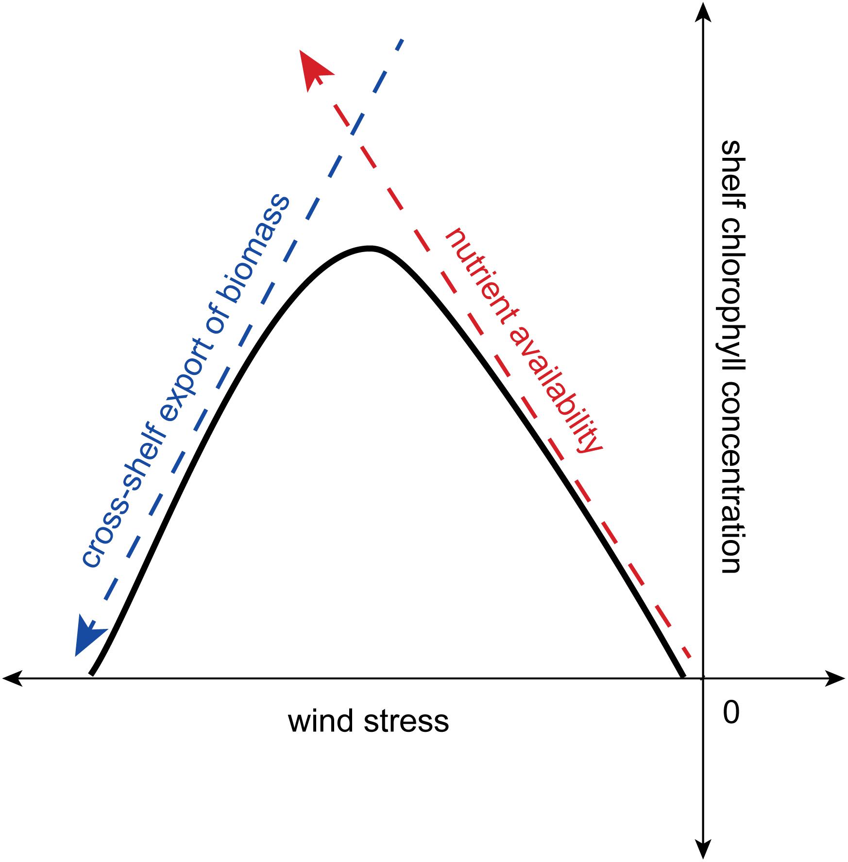
Figure 1. A conceptual diagram representing the Botsford et al. (2003) relationship. The relationship between shelf chlorophyll concentration and upwelling-favorable wind stress (black curve) results from the balance between the chlorophyll response to nutrient availability (red dashed arrow) and the chlorophyll response to cross-shelf export of biomass (blue dashed arrow).

In a later MLC model study, Botsford et al. (2006) found that variable winds (i.e., relaxation events) prolong time of phytoplankton on the shelf, allowing for more production and an increase in the optimal wind speed. Using a similar MLC model based on conditions observed in the CCS, Yokomizo et al. (2010) found that the optimal wind pattern for maximum productivity is wind that varies over a period equal to the shelf width divided by the cross-shelf velocity that results from the peak wind speed in the Botsford et al. (2003) relationship, and with the same mean cross-shelf velocity over the period. This finding implies that the optimal wind speed for maximum productivity varies with latitude and shelf width. More recently, in a more complex simulation built upon a traditional ECOPATH food web model that incorporates upwelling dynamics, Ruzicka et al. (2016) found that the dome-shaped relationship with upwelling strength exists across trophic levels. Specifically, their study found that phytoplankton, zooplankton, and secondary consumer fish all exhibited this pattern.

Furthermore, observational studies of the CCS have tended to corroborate the general suggestion in these model studies that increased upwelling does not lead to increased productivity in a simple, linear way. In an important paper, Ware and Thomson (2005) used satellite data spanning the whole CCS to characterize the mean distribution of productivity in CCS. They found that while Ekman transport offshore due to upwelling decreased with increasing latitude, productivity increased, with the most productivity found off of WA and BC where upwelling winds were the weakest. In a 2015 paper, Evans et al. (2015) attribute the failed bloom in July 2008 in Oregon on intense upwelling-favorable winds that pushed phytoplankton offshore before they could respond to upwelled nutrients. Based on observations within the CCS as part of the “Wind Events and Shelf Transport” program (WEST), Largier et al. (2006) found that increased upwelling-favorable wind strength leads to increased nutrient supply but excessive upwelling-favorable winds have a negative effect on productivity and lead to increased turbidity, increased offshore phytoplankton transport, deep mixing, and increased ammonium, which decreases nitrate uptake. However, when the duration of upwelling or relaxation events are on the order of phytoplankton blooms (several days), diatom blooms dominate the shelf region; when these events are longer, the shelves accumulate detritus and the phytoplankton move offshore. These findings suggest that the ideal conditions for productivity would be strong upwelling-favorable winds to bring nutrients to the euphotic zone, followed by a period of wind relaxation, with timescales on the order of phytoplankton blooms. This wind relaxation helps retain phytoplankton on the shelf, thus allowing the phytoplankton ample time to utilize the nutrients. Along the same lines, Hickey and Banas (2008) hypothesized that the intermittency of the winds in the Northern CCS was itself one of the drivers behind that region’s very high phytoplankton standing stock, with the intermittent winds interacting with freshwater plumes to boost retention and accumulation.

In a recent paper, Jacox et al. (2016) investigated bottom–up controls on productivity in the CCS using chlorophyll concentration observations from satellite combined with a realistic model. Like the previously described studies, their study used wind stress over the “nearshore” region (within 75 km of shore); however, they also included subsurface nitrate concentrations and the offshore region (75–300 km from shore) in their analysis. Their results suggest that in the nearshore region, maximum phytoplankton biomass results from moderate wind stress and high subsurface nitrate concentration, while in the offshore region, phytoplankton biomass is highly correlated with subsurface nitrate concentration. Offshore biomass is likely the result of advection of phytoplankton and nutrients from the nearshore region, although it is not significantly correlated with wind stress. Because of the non-linear interactions between wind strength and nutrient concentration, the relationship between productivity and one of these variables is dependent on the other and Jacox et al. (2016) found that one could not explain phytoplankton biomass by either one alone, nor with a combined metric such as vertical nitrate flux. The amount of nitrate available to upwell limits the maximum biomass attainable at a given wind stress, though this relationship varies across the ranges of wind stress and subsurface nitrate concentrations. These findings suggest a view in which in the nearshore region, phytoplankton biomass is dependent on both upwelling strength and characteristics of the upwelled water, while offshore phytoplankton biomass is only dependent on the characteristics of the upwelled water.

In past studies, productivity, including primary and higher trophic levels like fish, was often found to be correlated with indices representing upwelling variability, particularly the Upwelling Index (UI) (Bakun, 1973; Schwing et al., 1996) and Cumulative Upwelling Index (CUI) (Pierce et al., 2006) (e.g., Botsford and Wickham, 1975; Ware and Thomson, 2005). Overall, these indices are able to capture wind patterns in order to characterize the strength and variability of upwelling, but do not incorporate any measure of how characteristics of upwelling sourcewater, particularly its nutrient concentration, may have changed. However, as suggested by Jacox et al. (2016), both wind stress and subsurface nitrate concentrations are needed to characterize bottom–up controls on productivity. Recently, Jacox et al. (2018) created indices that include both the physical and nutrient dynamics: CUTI and BEUTI. CUTI (Coastal Upwelling Transport Index) represents the rate of vertical volume flux, while BEUTI (Biologically Effective Upwelling Transport Index) represents the vertical flux of nitrate into the mixed layer.

While there have been numerous investigations into the relationship between phytoplankton productivity and biomass and wind on the shelf, few have extended their analysis into the Northern part of the CCS. Fewer still have studied the influence of retention on this relationship. Using chlorophyll concentration and wind stress derived from satellite observations, we analyze the relationship between chlorophyll concentration and wind patterns in the Central and Northern CCS to see if the dome-shaped Botsford et al. (2003) relationship applies to the CCS as a whole and whether the Northern CCS is comparable or exhibits different behavior. In addition, we investigate how retention affects the relationship between chlorophyll concentration and wind stress in the Northern CCS using results from particle tracking experiments conducted in a model of the Northern CCS.

Materials and Methods

Satellite Chlorophyll Concentration and Wind Stress

For this study, we used chlorophyll concentration from a merged satellite product from the European Node for Global Ocean Color (GlobColour Project), which combines chlorophyll concentration observations from SeaWiFS (NASA), MODIS (NASA), MERIS (ESA), OLCI-A (ESA), and VIIRS (NOAA/NASA). The chlorophyll concentration data were 8-day composites spanning 1998 – Present at a 4-km spatial resolution. While only near-surface chlorophyll concentration is estimated by satellite, Frolov et al. (2012) found that depth-integrated chlorophyll is highly correlated with near-surface chlorophyll off of California (r² = 0.9), and so we will be using chlorophyll concentration as a proxy for phytoplankton biomass in this paper. This analysis focuses on the shelf region (from the coast to the 150 m isobath, shown in red in Figure 2). To address spatial variability, the shelf region was split into 1° latitudinal bands, over which we took the exponential of the mean of ln(chlorophyll concentration) to obtain a mean that is not as affected by large outliers, resulting in one time series for each degree over our entire domain, 35–50°N. This technique is useful, and commonly used, for datasets that are lognormally distributed like chlorophyll concentration (Campbell, 1995). Then 8-day chlorophyll concentration values were compared to 8-day mean wind stress (Figure 3). This timescale is appropriate for this analysis as it corresponds to timescales of both an upwelling event (3–10 days) (Hickey, 1979; Beardsley et al., 1987) and phytoplankton response time to upwelled nutrients (3–7 days) (Wilkerson et al., 2006). The 8-day mean wind stress values were derived from QuikSCAT and ASCAT satellite wind velocities from 1° longitude offshore following Smith (1988) (NOAA CoastWatch Program and Remote Sensing Systems, Inc.). Data span August 1999–November 2009 (QuikSCAT) and October 2009–Present (ASCAT) at a resolution of 0.25°. These data were then rotated parallel to the coastline throughout the study domain. To correspond with the chlorophyll concentration data, the mean of the wind stress data was taken over the same 1° latitudinal bands, with four data points within each band. For this study, we focused on the 2000–2019 time period, transitioning from QuikSCAT to ASCAT at November 1, 2009, over much of the Central and Northern CCS (35–50°N). These data were not calibrated to account for the different methods through which QuikSCAT and ASCAT make these measurements. Data from each sensors are differentiated in Figure 3 where mean 8-day composite chlorophyll concentrations are plotted against the corresponding mean 8-day wind stresses for each latitude. Bentamy et al. (2012) estimate the difference between wind speed measurements from QuikSCAT and ASCAT to be around 1 m/s, which corresponds to a wind stress of about 0.002 Pa. Given the resolution at which wind stresses are binned in further analysis (0.015 Pa bins; discussed below), we do not expect the difference between measurements from QuikSCAT and ASCAT to significantly affect our results and thus, measurements from QuikSCAT and ASCAT are no longer differentiated in later figures depicting wind stress.

FIGURE 2

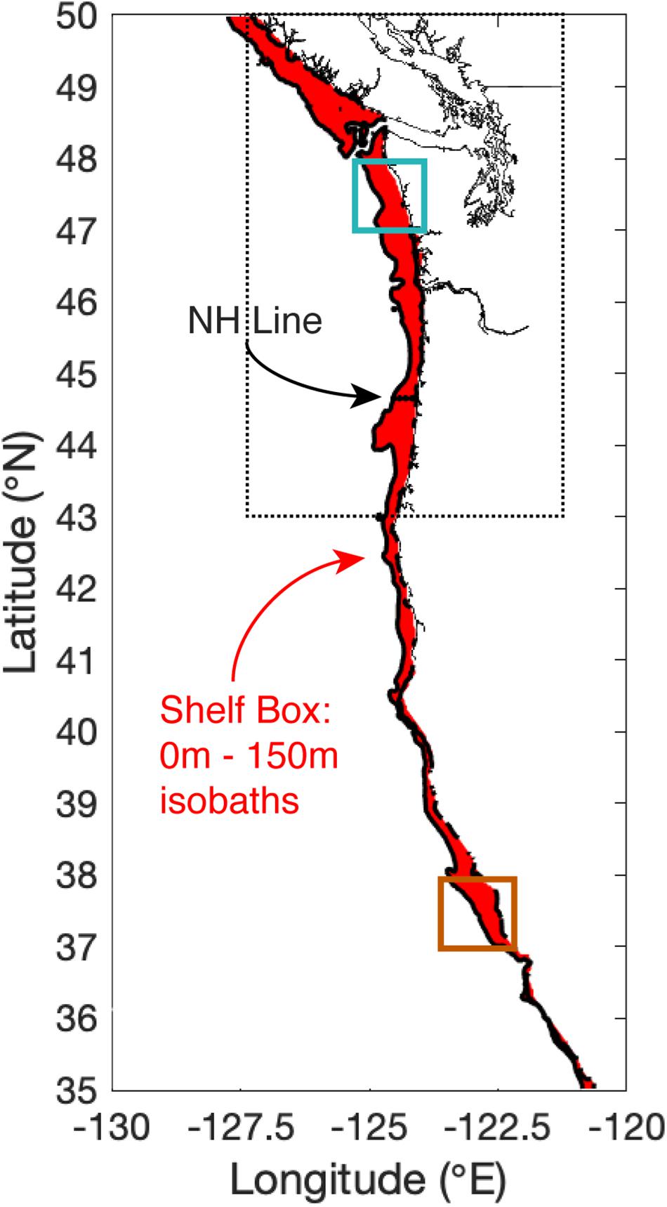
Figure 2. Study domain for the chlorophyll concentration and wind stress satellite data. The shelf (0–150 m isobaths) is shown in red. The Cascadia model domain used during the particle tracking experiments is outlined by the dashed line. Examples of latitude shelf boxes are shown in orange and cyan for 37.5°N (37–38°N) and 47.5°N (47–48°N), respectively. Black dots mark locations along the Newport Hydrographic Line used for satellite chlorophyll validation in Figure 4.

FIGURE 3

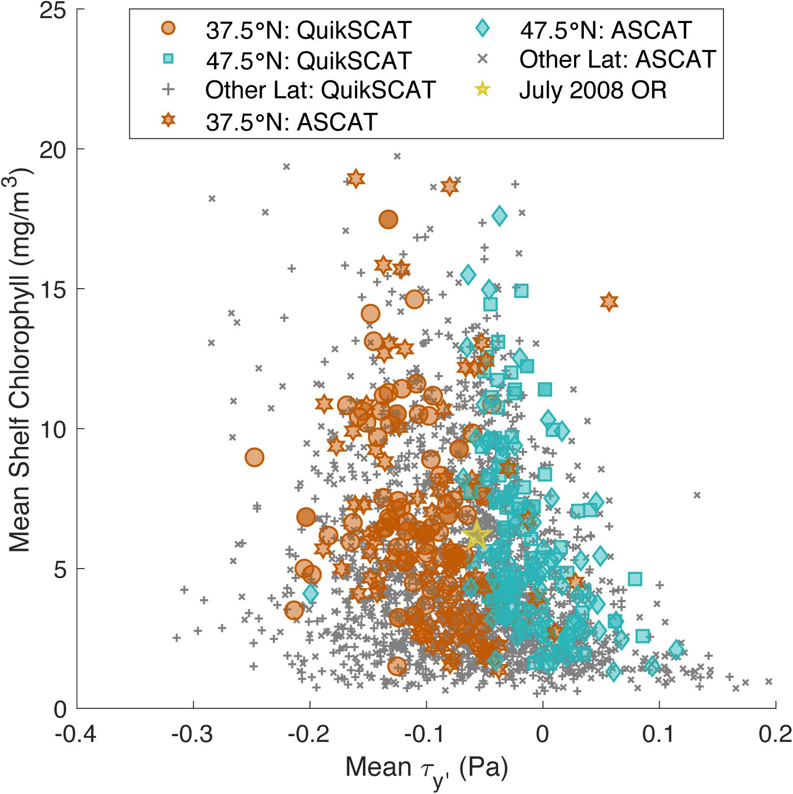
Figure 3. Mean 8-day composite shelf chlorophyll concentration plotted against its corresponding wind stress for each latitude from 35.5 to 49.5°N, with a distinction made between wind stresses derived from QuikSCAT measurements (January 2000–October 2009) and ASCAT measurements (November 2009–December 2019). Data from 37.5°N (between 37 and 38°N) is shown in orange circles (QuikSCAT) and orange hexagons (ASCAT), and data from 47.5°N (between 47 and 48°N) is shown in blue squares (QuikSCAT) and blue diamonds (ASCAT). The failed bloom in OR (44.5°N) in July 2008 (Evans et al., 2015) is depicted by the yellow star. All other latitudes are shown in gray crosses (QuikSCAT) and in gray Xs (ASCAT wind).

The GlobColour satellite product matches well with in situ observations within the study area. Surface bucket samples from the NOAA Newport Hydrographic (NH) Line (∼44.6° N) for the dates of January 2013 to February 2018 were compared to satellite color fields. NH Stations 1, 3, 5, 10, 15, and 20 (black dots in Figure 2) were used, which cover the width of the shelf and were sampled bi-weekly most of the year with monthly sampling in winter. Total samples for this time period varied by station from 54 to 92, with those stations closest to shore being sampled most often. Satellite chlorophyll concentrations were limited to a 1° latitude band centered on 44.6° N. Satellite and NH concentrations show a similar distribution, with a high proportion of low chlorophyll concentration values and a steep decline with increasing chlorophyll concentration (Figure 4A). A comparison of the mean of NH station values for each sampling date with the mean of satellite values over the Newport region for the corresponding 8-day period shows good agreement (r² = 0.34, p < 0.01; Figure 4B). For satellite wind validation, a recent study by Ribal and Young (2020) found that 10-m wind speed and direction measurements from both QuikSCAT and ASCAT match well with in situ 10-m wind speed and direction measurements from buoys located at least 50 km offshore from the National Data Buoy Center (ρ = 0.9593 and 0.9404, respectively), though QuikSCAT had a tendency to overestimate high wind speeds (>15 m/s). This study also compared wind speed measurements from four other satellite scatterometers and found generally good agreement among instruments, so we would expect similar results with these other satellite wind products.

FIGURE 4

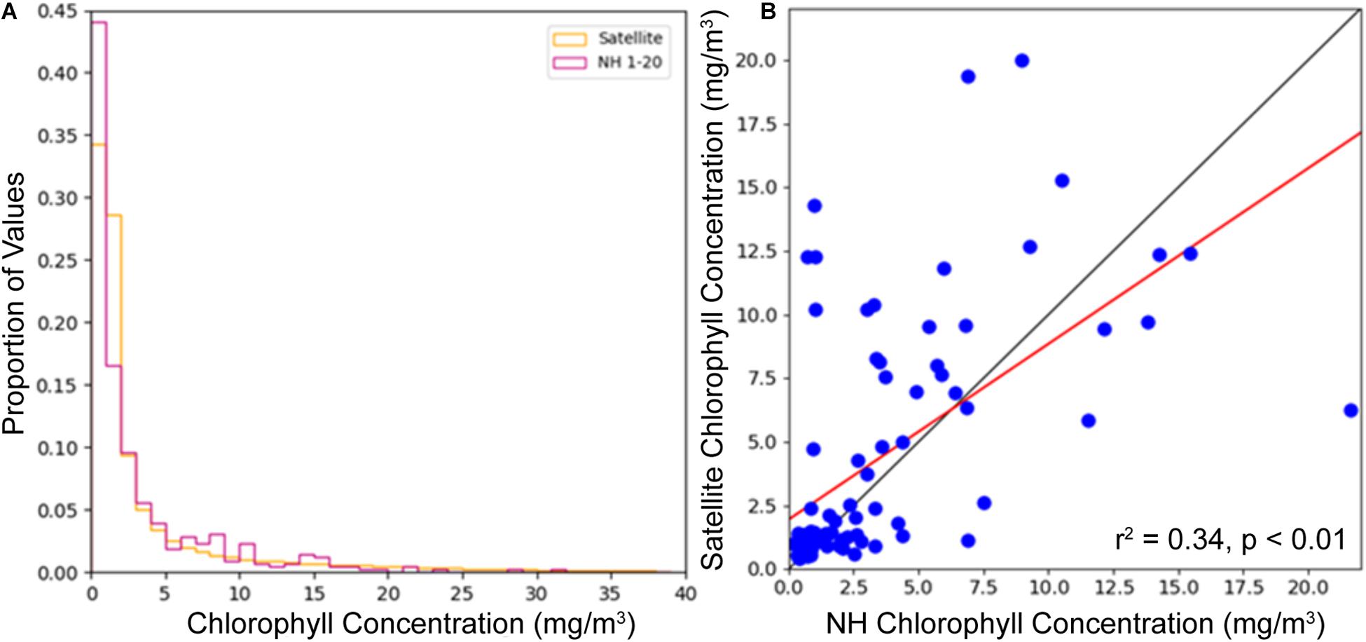
Figure 4. Comparison of GlobColour merged satellite product with in situ measurements taken along the Newport Hydrographic Line (NH) January 2013 through February 2018. Proportion of values histogram, where satellite values are 8-day composites over a 1° latitude band centered on 44.6°N while NH values are individual measurements for each station on each sample date (A). Scatter plot comparing the mean of NH stations sampled on each date with the mean of the satellite field for the Newport region for the corresponding 8-day composite (B), where the red line represents the trendline for the data, with an r² = 0.34, p < 0.01, while the diagonal gray line is 1:1.

Chlorophyll concentrations in each latitude band were binned by wind stress during the upwelling season (March–October). We took the natural log of chlorophyll concentration to calculate the 95% confidence intervals for each 0.015 Pa wind stress bin using the Student’s t-test (Emery and Thomson, 1997). Then, we plotted mean chlorophyll concentration vs. wind stress, as shown in the example plot in Figure 5, with the mean shelf chlorophyll concentration shown with the solid green line and the high and low 95% confidence intervals shown with the dashed green lines. Wind stress bins whose difference between the high and low 95% confidence intervals was greater than the global mean chlorophyll concentration (4.34 mg/m³; dashed black line in Figure 5) are colored in red, with the solid red line representing the mean and dashed red lines representing the high and low 95% confidence intervals. These red bins were ignored in the remainder of the analysis. By eliminating bins using these criteria, about 13% of observations are ignored as being too noisy and undersampled to analyze. Each latitude band was processed in this manner. This analysis was also conducted with NCEP Reanalysis winds (Kalnay et al., 1996) in place of QuikSCAT/ASCAT (see Supplementary Material), as well as with various upwelling season lengths with similar results (not shown). In particular, the analysis with NCEP Reanalysis winds showed a similar pattern when plotted against chlorophyll concentrations (Supplementary Figure S1), though NCEP wind stresses were often lower magnitude than QuikSCAT and ASCAT wind stresses, especially at high wind stresses, a pattern that was also reported in Fewings et al. (2016).

FIGURE 5

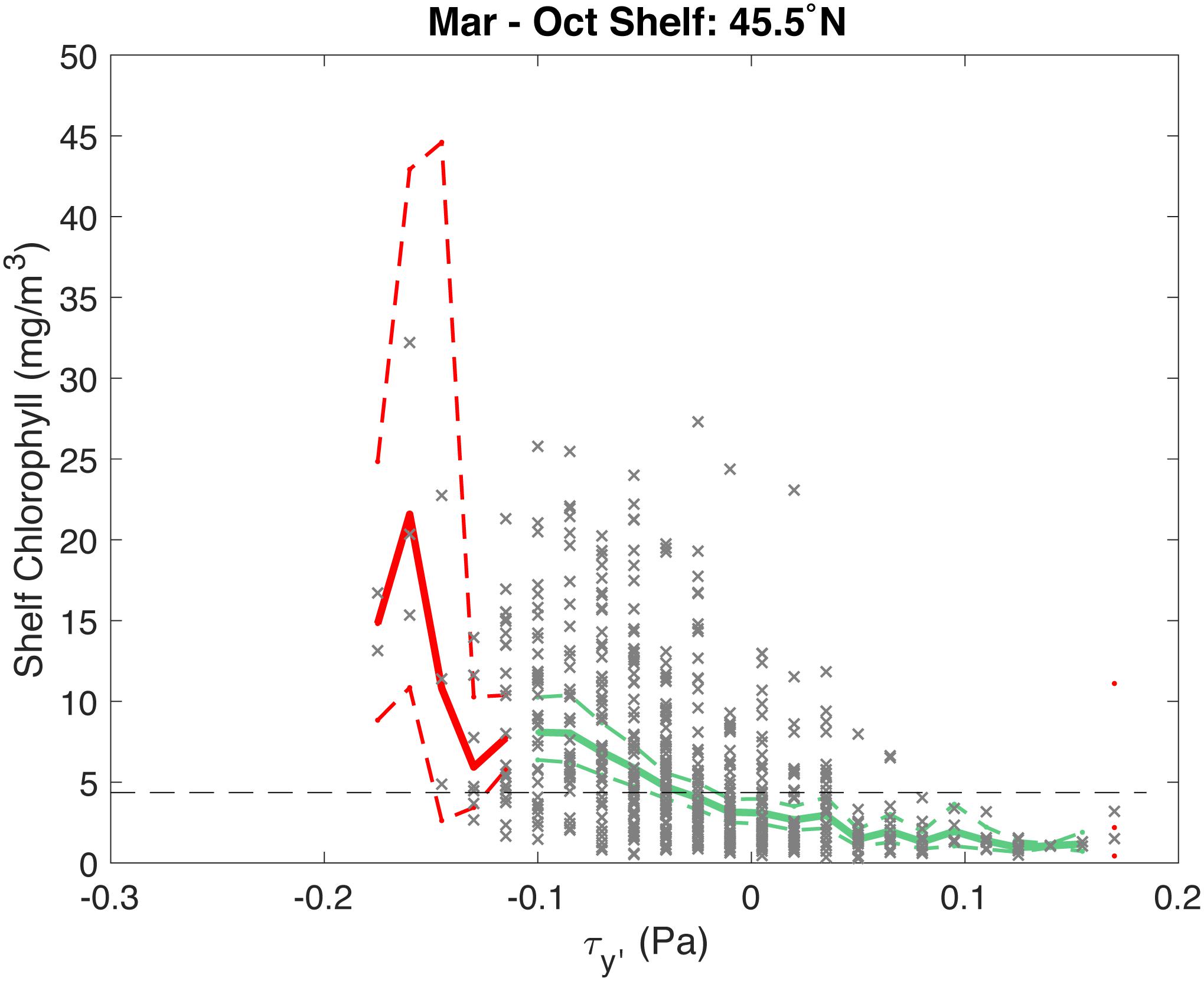
Figure 5. Example of chlorophyll vs. wind stress bins for the shelf at 45.5°N. The mean shelf chlorophyll concentration for each bin is plotted in the solid green line. The dashed green lines represent the 95% confidence intervals for each bin that is used in further analysis. The 8-day chlorophyll concentration data corresponding to each wind stress bin for this latitude band are plotted in gray. The dashed black line is the global mean shelf chlorophyll concentration (4.34 mg/m³). If the difference between the high confidence interval and low confidence interval for each bin was greater than the global mean (4.34 mg/m³), then that bin was ignored in further analysis; these bins are represented by the solid and dashed red lines, representing the mean and 95% confidence intervals for those bins.

Retention: Particle Tracking Experiments

To address the role of retention on the shelf, we conducted a particle release experiment in the Cascadia model developed by the Washington Coastal Modeling Group (Sutherland et al., 2011; Giddings et al., 2014) using the Regional Oceanic Modeling System (ROMS; Shchepetkin and McWilliams, 2005). The model domain includes the Salish Sea and coastal ocean of Washington, northern Oregon, and southern British Columbia (Figure 6). The horizontal resolution of the model over the slope and shelf is 1.5 km and expands out to a maximum of 4.5 km offshore. The model has 40 S-coordinate vertical layers, with stretching parameters set to better resolve the near-bottom and the upper water column. Ocean initial state and forcing on the southern and western boundaries are from the global Navy Coastal Ocean Model (NCOM; Barron et al., 2006, 2007). Rivers were forced by daily discharge data from the Columbia River, Fraser River, and 14 Puget Sound rivers using data from the USGS and Environment Canada (Giddings et al., 2014). Tides were provided by the quarter-degree TPXO7.2 inverse global tidal model (Egbert and Erofeeva, 2002). All atmospheric forcing was derived from the fifth-generation Mesoscale Model (MM5) from Pennsylvania State University–National Center for Atmospheric Research regional atmospheric forecast model [transitioning to the Weather Research and Forecasting model (WRF) in April, 2008] (Mass et al., 2003). A hindcast of physical parameters, including temperature, salinity, and velocity, spanning 2002–2009 was produced using this model setup, with each individual year 2002–2009 run in ROMS initialized from NCOM. Then each year 2003–2009 was re-run initialized from the previous year’s ROMS run, thus the year 2002 was discarded as spin-up. Overall, the model’s temperature, salinity, and sea surface elevation had high Willmott Skill Scores (WS ≥ 0.92; Willmott, 1982), based on comparison with data from 2264 CTD casts in 2005 (Giddings et al., 2014). More information about the Cascadia model can be found in Davis et al. (2014), Giddings et al. (2014), and Siedlecki et al. (2015), and more information about the particle tracking experiments can be found in Banas et al. (2009b) and Stone et al. (2018). Particles were released in on the shelf (i.e., in water shallower than 150 m, the depth of the shelf break) every 0.05° on the model domain (43–50°N) with release points plotted in black in Figure 6. They were released every 10 days over 2003–2009, resulting in 58,536 particles per year. Once released the surface-trapped particles were tracked with hourly time steps and daily output for up to 350 days, or until they moved outside the model boundaries or “beached” on land, defined as being close enough to land that a bilinear interpolation of the ROMS land mask (1 for ocean, 0 for land) at its location was less than 0.5 (Banas et al., 2015; Stone et al., 2018). Tidally-averaged model output was used for this particle release experiment. Retention times (T) were calculated for each particle based on how long it stayed on the shelf (shallower than 150 m). Examples of short retention times are plotted in blue and long retention times are plotted in red in Figure 6. Finally, median retention times were calculated for each latitude band from 44 to 49°N. For a given month and latitude, the monthly mean wind stress and monthly mean chlorophyll concentration, calculated from the same satellite-derived 8-day means used previously, were compared with the median retention time of particles that left the shelf during that month. This analysis was also conducted with particles in a depth-averaged surface layer ranging from 5 to 100 m to the surface, with similar results (not shown).

FIGURE 6

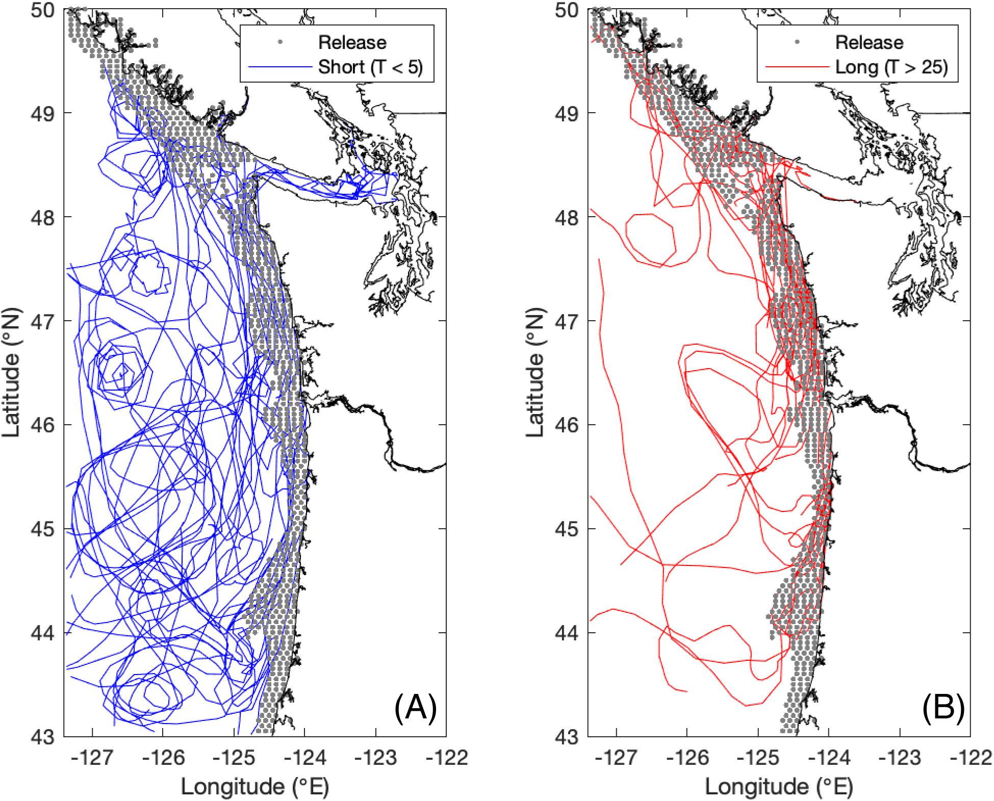
Figure 6. Model study domain for the particle tracking experiments. Particle release points are shown in gray. A subsample of particle tracks is also plotted, with short shelf retention times (T < 5 days) plotted in blue (A), and long shelf retention times (T > 25 days) plotted in red (B).

Results

Satellite Chlorophyll Concentration and Wind Stress

As expected in an Eastern Boundary Upwelling System, shelf chlorophyll concentrations were generally highest during negative (upwelling-favorable) meridional wind stress (Figure 3). In Figure 3, data from the Central CCS, including from 37.5°N (plotted in orange), makes up the left side of the figure, while data from the Northern CCS, including from 47.5°N (plotted in blue), makes up the right side of the figure. This pattern shows the strong upwelling-favorable winds that are typical in the Central CCS, as well as the weaker upwelling-favorable winds that are typical in the Northern CCS. However, the same chlorophyll concentration can result from different wind stresses in the Central and Northern CCS, suggesting a varied relationship between chlorophyll concentration and wind stress throughout the CCS. For example, there are numerous observations of chlorophyll concentrations between 15 and 20 mg/m³ at wind stresses ranging from −0.3 to 0 Pa (Figure 3). While these observations are some of the highest chlorophyll concentrations observed over the record, they were measured during a wide range of wind stresses, including some of the strongest and weakest upwelling-favorable winds from the record.

Calculating the mean chlorophyll concentration that occurs under a particular wind stress by latitude further suggests that while wind stress is important to chlorophyll concentration throughout the domain, other mechanisms alter how this relationship manifests, particularly in the Northern CCS. For example, in the south, this relationship is roughly flat, particularly at 35.5 and 39.5°N (dark red and orange, respectively; Figure 7). However, as latitude increases, this relationship progresses toward a monotonic relationship, with highest chlorophyll concentrations at the most upwelling-favorable winds, for example 46.5 and 47.5°N (teal and blue, respectively; Figure 7). For each latitude, chlorophyll concentration increases with increasing upwelling-favorable wind, while for a given wind stress, chlorophyll concentration increases with latitude, as evidenced at about −0.05 Pa (Figure 7).

FIGURE 7

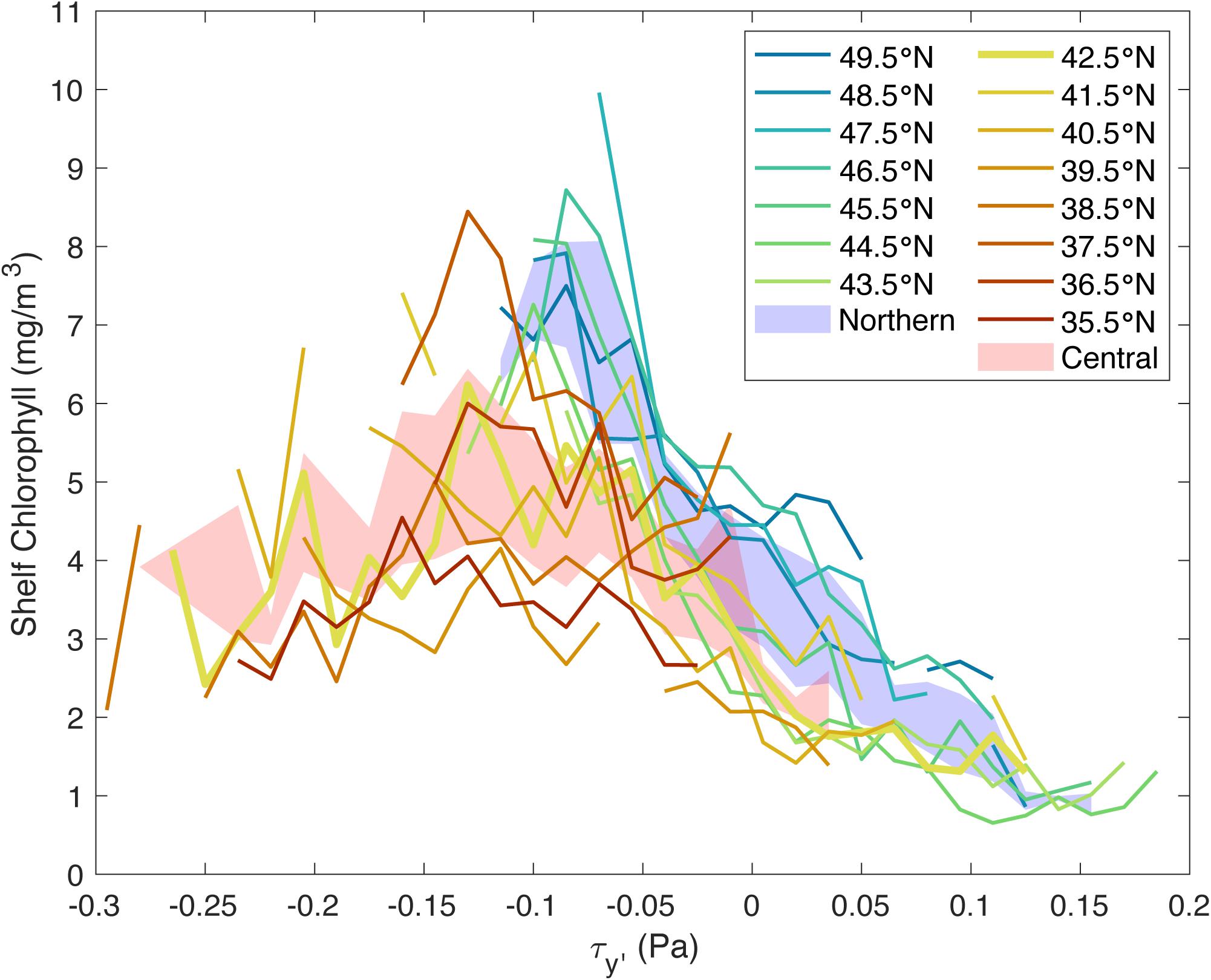
Figure 7. Shelf chlorophyll concentration vs. wind stress bins for the entire domain (35.5–49.5°N) from 2000 to 2019, colored by latitude. Only bins whose difference between high and low 95% confidence intervals is less than the global shelf chlorophyll mean are included. Northern latitudes (43.5–49.5°N) are shown in cool colors, while Central latitudes (35.5–41.5°N) are shown in warm colors, with the dividing latitude (42.5°N) is shown in the thick yellow line. Mean chlorophyll concentration vs. wind stresses curves are plotted for the Central region (35.5–42.5°N; shaded red) and Northern region (43.5–49.5°N; shaded blue). These mean curves were calculated via the bootstrapping method in MATLAB and are plotted to depict the 95% confidence intervals for each region.

Individually, results at any single latitude do not support the Botsford et al. (2003) relationship, except perhaps at 42.5°N (bold yellow line; Figure 7) where there is a hint of a dome-shaped relationship between wind stress and chlorophyll concentration. However, over the whole CCS, the relationship between chlorophyll concentration and wind stress has a dome-shaped envelope, consistent with the Botsford et al. (2003) relationship, with individual latitudes contributing different parts of the dome. In the Central CCS (warm colors), the chlorophyll concentrations appear to peak at a wind stress of about −0.125 Pa (Figure 7), while in the Northern CCS (cool colors), the chlorophyll concentrations appear to peak at a wind stress of about −0.05 Pa (Figure 7). Furthermore, the Central and Northern regions have significantly different relationships between mean chlorophyll concentration and wind stresses. This difference is evident in the separation between the mean curves for the Central and Northern regions, which were calculated via the bootstrapping method in MATLAB and are plotted to depict the 95% confidence intervals for the Central (red shaded curve) and Northern (blue shaded curve) regions (Figure 7). While these curves do overlap at a few points near 0 Pa, the rest of points are significantly different.

The difference in chlorophyll concentration-wind stress curves for the Central and Northern regions suggests two dynamically distinct systems north and south of 42.5°N, which experiences almost the full range of wind stresses. The location of this split is consistent with previous work that found that Cape Blanco (41.9°N) divided the upwelling system into two regimes: one that is influenced by the Columbia River plume on the shelf north of Cape Blanco and one that is more influenced by strong upwelling-favorable winds south of Cape Blanco (Huyer et al., 2005). The Central CCS appears to be governed by traditional coastal upwelling dynamics characterized by the Botsford et al. (2003) relationship, while in the Northern CCS, the Botsford et al. (2003) relationship manifests differently, with high chlorophyll concentrations observed even during weak upwelling-favorable winds. Furthermore, unlike the Central CCS, the Northern CCS has high chlorophyll concentrations during positive (downwelling-favorable) wind stresses (Figures 3, 7). Often, particularly for 46.5–48.5°N, the mean chlorophyll concentration at positive wind stresses are almost as large as the greatest mean chlorophyll concentrations observed in the Central CCS. However, while phytoplankton in the Northern CCS are productive during downwelling-favorable wind events, this behavior is only observed during the upwelling season. Previous studies have found that phytoplankton will exhibit a large negative productivity anomaly in the event of an anomalously late spring transition like in 2005 (Hickey et al., 2006; Kudela et al., 2006). Still, the overall pattern in the Northern CCS goes against the traditional upwelling-driven phytoplankton productivity that is characteristic of the CCS and suggests another mechanism supporting phytoplankton productivity in the Northern CCS during the upwelling season.

As noted in the Introduction, Hickey and Banas (2008) present two hypotheses for why the Northern CCS is productive at weaker wind stresses: (1) shelf retention related to wind intermittency, freshwater plume dynamics, and shelf geometry, and (2) non-upwelling-derived nutrient sources. Increased retention on the shelf at a given mean wind stress would allow phytoplankton more time to use upwelled nutrients, potentially resulting in higher chlorophyll concentrations at lower wind stresses, particularly on the falling (highly negative wind stress) side of the dome-shaped curve. If this mechanism explained the difference between the Northern and Central CCS in our results, it would manifest itself as either higher retention times at a given moderate wind stress or a more complicated, scattered relationship between retention time and wind stress in the Northern region. Furthermore, to support this hypothesis, this effect of wind intermittency on retention would outweigh the linear relationship between downwelling-favorable winds (positive wind stress) and retention time that represents retention due to Ekman transport onshore driven by downwelling-favorable winds. By conducting particle tracking experiments in a ROMS model, we were able to test this hypothesis.

Influence of Shelf Retention

After calculating retention times from each particle track, monthly median retention times were plotted against monthly mean meridional wind stress. In general, rather than exhibiting either a peak in retention time at moderate wind stress or a scattered relationship between retention time and wind stress that would represent the relationship between high retention time and wind intermittency, in the Northern CCS, retention times increase with positive, downwelling-favorable wind stress, and there appears to be very little variance in this relationship with latitude (r² = 0.35 ± 0.11, p < 0.01; Figure 8A). The linear relationship between wind stress and retention time suggests that on this scale (1° latitude bins), the effect of wind intermittency on retention time is minimal. Overall, it seems likely that on a large scale, retention is largely driven by the simple mechanism of downwelling-favorable winds inducing Ekman transport onshore, rather than the more nuanced causes of retention such wind intermittency, geography, and mesoscale features as put forth in Hickey and Banas (2008). However, this analysis cannot reject the hypothesis that mesoscale features in the Northern CCS interact with wind intermittency (Hickey and Banas, 2008; Banas et al., 2009c) in ways that affect the region’s mean productivity (Figure 7) more strongly than they affect mean retention time (Figure 8). If this were the case, it would not be discernible in retention calculations on this 1° latitude-wide scale.

FIGURE 8

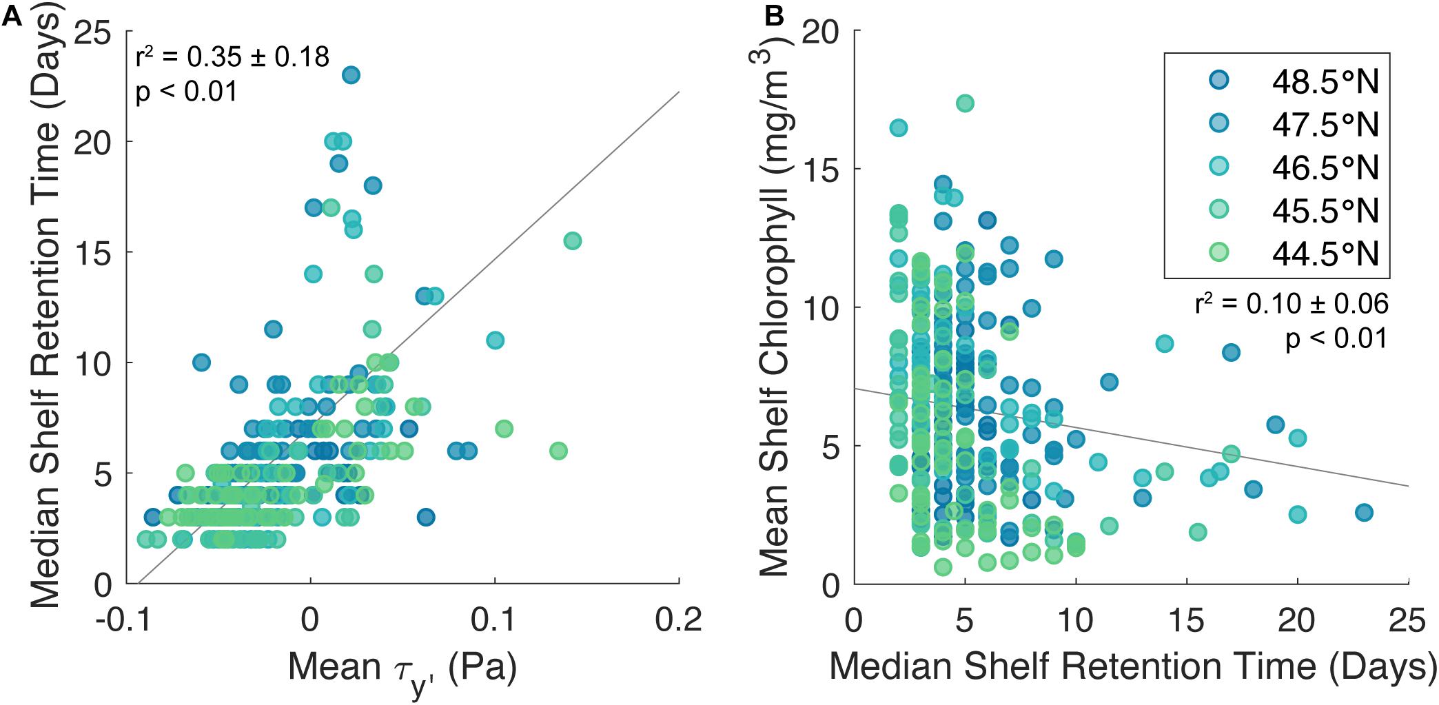
Figure 8. Monthly median shelf retention time plotted against mean wind stress (A) and monthly mean shelf chlorophyll concentration plotted against median shelf retention time (B) for 2003–2009. Results from 44.5°N through 48.5°N are colored by latitude, with more northern latitudes in blues and more southern latitudes in greens. Trendlines for each relationship are plotted in gray [r² = 0.35 ± 0.11, p < 0.01 (A); r² = 0.10 ± 0.06, p < 0.01 (B)]. There are five instances of retention times > 25 days that are left off this figure in the interest of resolution of the low retention values. In this figure, retention times (T) are calculated from model output while wind stress and chlorophyll concentrations are calculated from the same satellite data used previously.

Comparison With CUTI and BEUTI

We also compared the satellite chlorophyll concentration data with the new upwelling indices CUTI and BEUTI from Jacox et al. (2018), both of which are based on estimates from a data-assimilative ROMS reanalysis model of the CCS spanning 1988 to present from 31 to 47°N. CUTI (Coastal Upwelling Transport Index) quantifies the rate of vertical volume transport and includes both Ekman transport and cross-shelf geostrophic flow. BEUTI (Biologically Effective Upwelling Transport Index) quantifies the vertical nitrate flux into the mixed layer, based on CUTI and concentration of nitrate below the mixed layer. Thus, as defined, BEUTI does not include lateral nutrient fluxes into the mixed layer. If the higher productivity of the Northern CCS is due to higher nutrient concentrations below the mixed layer such that a weaker wind stress would still result in a high concentration of nutrients upwelled, then we would expect a plot of chlorophyll concentration against BEUTI to collapse the two peaks into one peak. More information about these indices can be found in Jacox et al. (2018) and at http://mjacox.com/upwelling-indices/.

As expected, shelf chlorophyll concentration increases with increasing CUTI, with the Central CCS experiencing the highest values for CUTI and the Northern CCS experiencing the lowest values (Figure 9A). Similar to the patterns in Figure 7, the relationship between shelf chlorophyll concentration and CUTI suggests variation with latitude, as in the Northern CCS, some of the highest chlorophyll concentrations correspond to the lowest CUTI values over the whole CCS. Overall, the use of CUTI does not help explain the difference between the Central and Northern CCS by collapsing the two peaks in chlorophyll concentration for the different regions into one peak, likely because CUTI represents wind-driven vertical transport into the mixed layer.

FIGURE 9

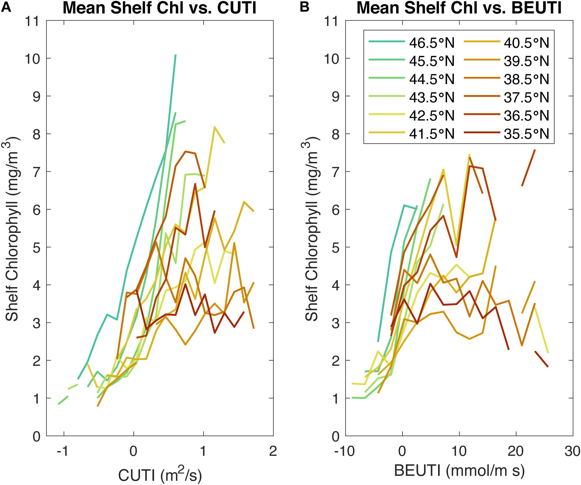
Figure 9. Mean shelf chlorophyll concentration plotted against CUTI (A) and BEUTI (B), colored by latitude. Similar to the shelf chlorophyll concentration vs. wind stress plots, in these plots, shelf chlorophyll was binned by its corresponding CUTI and BEUTI values, and the mean value and 95% confidence intervals for each bin is calculated. For CUTI, each bin represents 0.14 m²/s and for BEUTI, each bin represents 2.3 mmol/s. Bins with a difference between their high and low confidence intervals greater than the CCS-wide mean were ignored.

Similarly, the Central CCS experiences the highest BEUTI values, while the Northern CCS experiences the lowest values, once again crossing into negative BEUTI values (Figure 9B). There appears to be some separation between the Northern CCS and Central CCS in the shelf chlorophyll plotted against BEUTI. This separation suggests that it is not a higher subsurface nutrient concentration that accounts for the higher chlorophyll concentrations in the Northern CCS. These results suggest that is more likely that the BEUTI index does not capture the different nutrient dynamics in the Northern CCS, such as the lateral nutrient flux via outflow from the Salish Sea (Davis et al., 2014), in the sense that if BEUTI captured those mechanisms, the Northern and Central relationships would collapse together.

Discussion

While the overall relationship between shelf chlorophyll concentration and wind stress is dome-shaped for the entire Central and Northern CCS, as suggested by Botsford et al. (2003) and supported by Yokomizo et al. (2010), Jacox et al. (2016), and Ruzicka et al. (2016), this is not the case for individual latitudes within the CCS, likely because each individual latitude band does not experience enough wind variation, or because strong winds occur so rarely during the satellite era that we cannot resolve them statistically (Figures 5 and 7). In particular, in the Northern CCS, the relationship between shelf chlorophyll concentration and wind stress is most simply described as monotonic, with the highest chlorophyll observations occurring with the most upwelling-favorable (negative) wind stress values. However, the Northern CCS does not typically experience the most extreme upwelling-favorable wind stress observed in the CCS. If stronger upwelling-favorable winds became common and statistically resolvable in the Northern region, would chlorophyll concentrations decrease, as suggested by Botsford et al. (2003), or would they continue to increase? This uncertainty presented by lack of forcing variability extends into the Central CCS as well, where there are few observations of the most extreme winds. Of those observations, the phytoplankton response varied widely, evident in Figure 3 where wind stresses beyond −0.25 Pa elicited chlorophyll concentrations ranging from about 2 to 22 mg/m³. However, due to the statistical limits accompanying few observations, we cannot say anything meaningful about these extreme winds. The results presented in Figure 7 represent about 87% of all observations for the Central and Northern CCS and these results support the application of Botsford et al. (2003)’s dome-shaped relationship for the CCS as a whole.

While the simple dome-shaped relationship does appear to apply to the CCS as a whole, there are some limits to this interpretation of the wind-productivity relationship. Botsford et al. (2003) only considers a simple, two-dimensional upwelling system, but does not consider regional differences, such as the role of filaments in the Central CCS and the role of freshwater input and non-upwelling-derived nutrients sources in the Northern CCS. This two-dimensional upwelling system includes cross-shelf transport but does not include any downstream transport, which is particularly relevant in the presence of filaments. The semi-permanent filaments of the Central CCS form at capes and other promontories and act as a rapid conduit of phytoplankton to the open ocean, particularly at Pt. Arena (38.9°N) and Cape Mendocino (40.4°N) (Strub et al., 1991). The rapid transport of chlorophyll offshore by these filaments could explain the flatness of the 38.5 and 40.5°N lines in Figure 7 that depict their relationship between wind stress and chlorophyll concentration. Inclusion of both cross-shelf and downstream transport in the Botsford et al. (2003) model might better capture the relationship between chlorophyll concentration and wind stress in this upwelling system, and is an important direction for future work.

If chlorophyll concentration decreases on the shelf under extreme wind conditions because of cross-shelf advection, one might expect significant chlorophyll concentrations observed in the offshore region under strong upwelling. Previous studies suggest that beyond the shelf break, phytoplankton are less productive due to both limited light and nutrient availability. Huntsman and Barber (1977) found that phytoplankton become light-limited during periods of deep mixing, reducing the overall productivity of the region during a mixing event lasting just days. Additionally, subduction and advection of nutrients and phytoplankton from the coast to the open ocean via mesoscale eddy activity (Rossi et al., 2008, 2009; Gruber et al., 2011) and by the California Current jet (Barth et al., 2002) reduces productivity near the coast. However, a model study by Lathuilière et al. (2010) found that while overall productivity of the shelf region decreases due to transport of nutrients and phytoplankton offshore, mesoscale eddy activity widens the coastal productivity band from about 80 km to 200 km, suggesting that phytoplankton can still be productive in the offshore region. Additionally, Jacox et al. (2016) found that the offshore region was still productive, though less so than the shelf region because chlorophyll concentration in the offshore region is about 12–25% of that of the shelf region, but this productivity was not significantly correlated with wind stress. Our initial analysis examined chlorophyll concentration in the offshore region (between the 150 and 2500 m isobaths) using a similar procedure as we used for the shelf region. Similar to Jacox et al. (2016), based on plots from all latitudes spanning 35–50°N, the chlorophyll concentrations in the offshore region were about 25% of those of the shelf region and remain roughly constant with varying wind stress (not shown).

However, it may not be the case that phytoplankton productivity in this offshore region is a minor contribution, as these studies suggest. Other studies have found that in the offshore region, a subsurface chlorophyll maximum may develop due to subduction of phytoplankton offshore (Kadko et al., 1991; Barth et al., 2002; Bograd and Mantyla, 2005; Huyer et al., 2005), and this feature likely is not captured by satellite in the offshore region. Furthermore, there is also evidence that in the offshore region, phytoplankton shift to a smaller cell size due to iron limitation and these smaller phytoplankton are more tightly coupled with grazers (Rykaczewski and Checkley, 2008). If future work is able to incorporate more observations of phytoplankton under extreme upwelling-favorable wind conditions, it would be useful to examine the offshore region as well to see if there is a transfer to phytoplankton offshore from the shelf, or if once phytoplankton leave the shelf, they are largely lost to the depths.

Lastly, results from the particle release experiment found that on a large, 1° latitude-wide scale, the effect of wind intermittency on retention is minimal because the relationship between retention time and wind stress is linear. However, this result does not disqualify the influence of more complex controls on retention like wind intermittency on smaller spatial scales. The interactions between intermittent winds, mesoscale bathymetry (e.g., Heceta Bank), and freshwater dynamics (e.g., the Columbia River plume) could easily lead to a situation in which mesoscale, transient retention features had a greater effect on large-scale mean chlorophyll concentrations than on large-scale mean shelf retention times. Pursuing these possibilities likely requires a Lagrangian analysis of nutrient and biomass budgets, presumably in models, rather than an Eulerian, observational analysis.

The same small-scale features might well have equally non-linear effects on large-scale mean nutrient supply. The Columbia River plume entrains ocean-derived nutrients though mixing between ocean water and river water at the river plume lift-off region and then moves these nutrients seaward at the surface (Hickey and Banas, 2008; Banas et al., 2009a; MacCready et al., 2009). Similarly, nutrient-rich water that is upwelled into the Strait of Juan de Fuca is entrained into the surface outflow, spreading nutrients along the shelf locally (Hickey and Banas, 2008; MacFadyen et al., 2008; Davis et al., 2014). Additionally, irreversible turbulent mixing throughout the region transports nitrate from near-bottom water to surface water at a rate of about 25% of nutrient transport by upwelling (Hales et al., 2005). Therefore, in addition to retaining phytoplankton in surface shelf water, the mechanisms within these “retentive regions” may be providing more nutrients to the shelf via entrainment of ocean-derived nutrients into the surface layer.

Conclusion

Using chlorophyll concentration and wind stress derived from satellite observations, we studied the relationship between chlorophyll concentration and wind stress in the CCS, spanning 35 to 50°N, and 2000–2019. Additionally, to address the influence of shelf retention on this relationship, we conducted particle tracking experiments in a ROMS model of the Northern CCS (43–50°N) for 2003–2009. The main conclusions for this analysis are:

(1) The relationship between chlorophyll concentration and wind stress in the California Current System is dome-shaped.
Does the Botsford et al. (2003) relationship apply to the Central and Northern California Current System? Yes, but only as a whole. At individual latitudes, only pieces of the dome-shaped relationship between chlorophyll concentration and wind stress are visible (Figure 7). In general, at a given latitude, chlorophyll concentration increases with upwelling-favorable wind stress, with a downturn in chlorophyll concentration at high upwelling-favorable wind stresses in the Central CCS. At a given wind stress, chlorophyll concentration increases with latitude with the Northern CCS having the highest chlorophyll concentrations. Additionally, in the Northern CCS, chlorophyll concentrations were still relatively high during downwelling-favorable winds.

(2) High chlorophyll concentration is observed in the Northern CCS during weak upwelling-favorable and downwelling-favorable winds.
Despite the weaker upwelling-favorable winds, as well as downwelling-favorable winds experienced during the upwelling season, high chlorophyll concentrations are observed in the Northern CCS (Figure 7). In fact, over the entire CCS, some of the highest chlorophyll concentrations are observed in the Northern CCS, despite the weaker winds, as Ware and Thomson (2005) originally noted, using a much shorter satellite record.

(3) There are two separate curves that describe the relationship between chlorophyll concentration and wind stress in the CCS.
The Central CCS and Northern CCS have significantly different relationships between mean chlorophyll concentration and wind stresses, which is evident in the separation between the mean curves for the Central (red shaded curve) and Northern (blue shaded curve) regions (Figure 7). These results suggest that the Central CCS is governed by traditional upwelling dynamics, while the high chlorophyll concentrations during weak upwelling-favorable and downwelling-favorable winds in Northern CCS suggests another mechanism supporting phytoplankton productivity during the upwelling season. Hickey and Banas (2008) present two hypotheses for the Northern CCS’s high biomass: complex retention on the shelf and additional non-upwelling-derived nutrient sources. Their second hypothesis is further supported by Davis et al. (2014), who found in a model study that the nutrient-rich outflow from the Strait of Juan de Fuca fueled productivity in this region. While results from the particle tracking experiment compared with chlorophyll concentrations and wind stress in the Northern CCS found that the effect of wind intermittency on retention is minimal on a 1°latitude-wide scale (Figure 8), they do not disqualify the influence of more complex controls on retention like wind intermittency on smaller spatial scales.

Based on these results, we propose a revised Botsford et al. (2003) relationship for the CCS (Figure 10). The Central CCS is governed by traditional upwelling dynamics and its relationship between shelf chlorophyll concentration and wind stress (orange curve; Figure 10A) represents the balance between nutrient availability (red dashed arrow; Figure 10A) and cross-shelf export of biomass (blue dashed arrow; Figure 10A). The Northern CCS still follows the overall pattern of traditional upwelling dynamics, with its relationship between shelf chlorophyll concentration and wind stress (teal curve; Figure 10B) still representing this balance, but its nutrient availability is increased by non-upwelling-derived nutrients (teal arrow; Figure 10B). Non-upwelling-derived nutrient sources include lateral nutrient fluxes through mechanisms like outflow from the Salish Sea which Hickey and Banas (2008) estimated as 0.6 × 10⁹ kg of nitrate per upwelling season and which Davis et al. (2014) suggests account for 20% of primary productivity in the Northern CCS, with contributions varying with distance from the Strait of Juan de Fuca. Outflow from the Columbia River also contributes to non-upwelling-derived nutrients (0.04 × 10⁹ kg of nitrate per upwelling season: Hickey and Banas, 2008), though its effects are much more localized and are on a smaller scale (Davis et al., 2014). This increase in nutrient availability in the Northern CCS effectively shifts the chlorophyll-wind relationship toward downwelling-favorable wind stresses, resulting in the high productivity at weak upwelling-favorable and downwelling-favorable winds that is characteristic of the Northern CCS. While the data from the Northern CCS do show that chlorophyll concentration is higher on the falling side of the curve in downwelling-favorable wind stresses, the shape of the curve on the high chlorophyll side in upwelling-favorable wind stresses is unclear (Figure 7). Therefore, the data are consistent with this revised Botsford et al. (2003) relationship for the CCS, but they are not sufficient to fully test this new hypothesis.

FIGURE 10

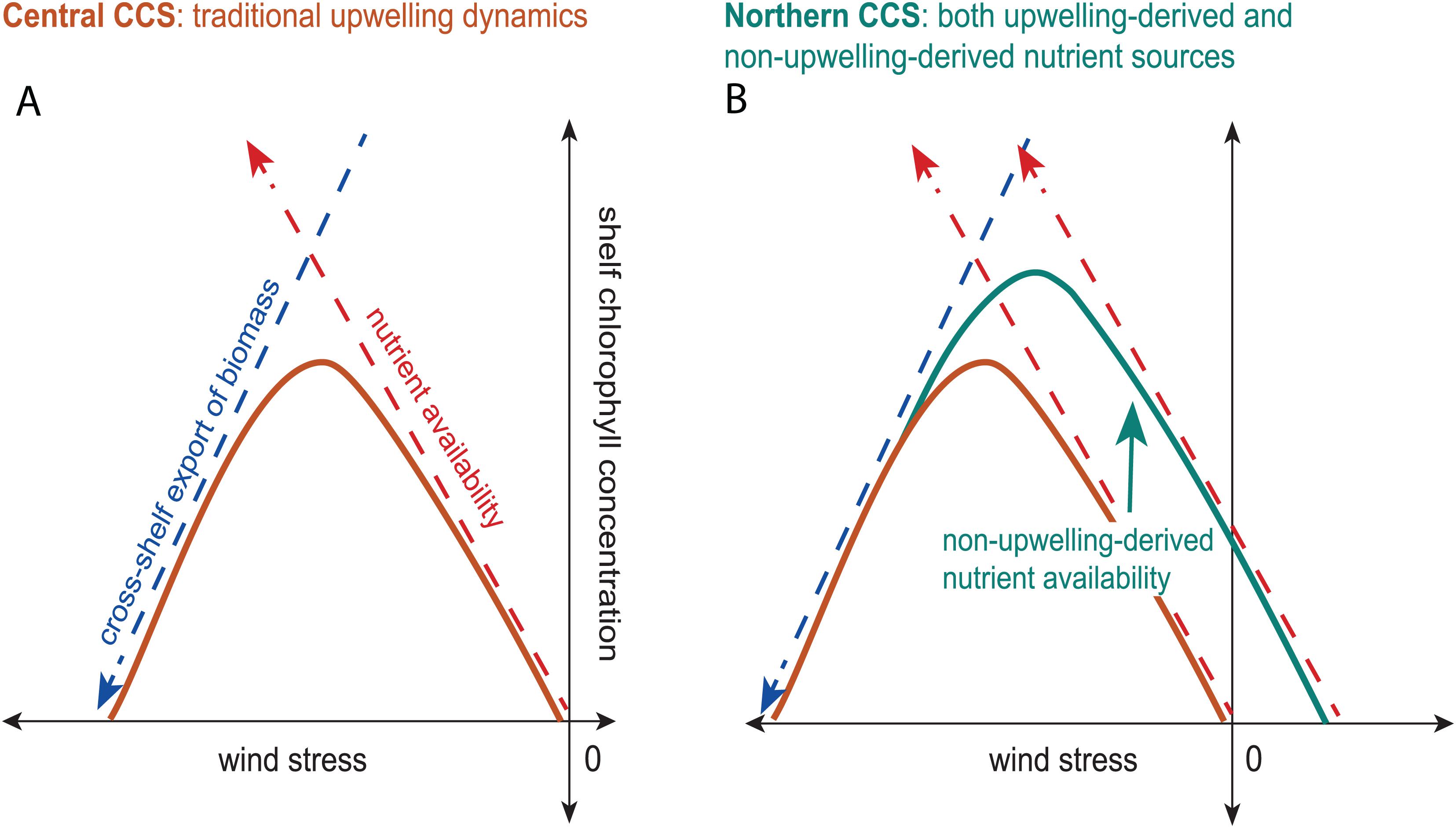
Figure 10. A revised Botsford et al. (2003) relationship for the Central and Northern CCS. The relationship between shelf chlorophyll concentration and wind stress in the Central CCS (orange curve, A) and in the Northern CCS (teal curve, B). The chlorophyll response to nutrient availability supplied by upwelling-favorable wind stress is depicted by the red dashed arrow, while the chlorophyll response to cross-shelf export of biomass is depicted by the blue dashed arrow. Non-upwelling-derived nutrient availability (teal arrow in B) in the Northern CCS accounts for the increase in overall nutrient availability and shift of the shelf chlorophyll response to wind stress (teal curve) into downwelling-favorable wind stresses (B).

Future work should focus on understanding the role of mesoscale retention driven by geographic features and wind intermittency, as well as the role of lateral nutrient fluxes in the Northern CCS, such as outflow from the Strait of Juan de Fuca and river discharge. Incorporation of these non-upwelling-derived nutrient sources into indices like CUTI and BEUTI could help collapse the observations into Botsford et al. (2003)’s hypothesized dome-shaped relationship as expected. Furthermore, a better understanding of the nutrient-chlorophyll dynamics in the Northern CCS may allow us to better predict how productive this region may be under different future conditions.

Data Availability Statement

The raw data supporting the conclusions of this article will be made available by the authors, without undue reservation.

Author Contributions

HS, NB, and PM contributed conception and design of the study. HS did most of the analysis, with assistance from BO. HS wrote the first draft of the manuscript with NB, PM, and RK providing editorial edits. All authors contributed to manuscript revision, read and approved the submitted version.

Funding

HS was supported by a National Science Foundation (NSF) Graduate Research Fellowship. PM, NB, and HS were supported by MERHAB grant number NA16NOS4780189 from the Coastal Ocean Program of the National Oceanic and Atmospheric Administration (NOAA). RK was supported by the RISE funds from NSF, grant number OCE 0238347. BO was supported by NOAA grant number NA16NOS0120019. This work was part of HS graduate research at the University of Washington. This was contribution 225 of the MERHAB program. The findings and conclusions are those of the authors and do not necessarily reflect those of NSF, NOAA, or the Department of Commerce.

Conflict of Interest

The authors declare that the research was conducted in the absence of any commercial or financial relationships that could be construed as a potential conflict of interest.

Acknowledgments

Special thanks to the PM and NB lab groups for useful conversations, to Melanie Fewings for help with satellite wind products, to Mike Jacox for use of the CUTI and BEUTI indices, to Kym Jacobson and Jennifer Fisher at NOAA Northwest Fisheries Science Center for providing the Newport Hydrographic Line data, to Evelyn Lessard for guidance, and to David Darr for computer cluster administration and support.

Supplementary Material

The Supplementary Material for this article can be found online at: https://www.frontiersin.org/articles/10.3389/fmars.2020.551562/full#supplementary-material

References

Allen, S. E., and Hickey, B. M. (2010). Dynamics of advection-driven upwelling over a shelf break submarine canyon. J. Geophys. Res. 115:C08018. doi: 10.1029/2009JC005731

CrossRef Full Text | Google Scholar

Bakun, A. (1973). Coastal Upwelling Indices, West Coast of North America. NOAA Technical Report, NMFS SSRF-671. Washington, DC: US Department of Commerce.

Google Scholar

Banas, N. S., Conway-Cranos, L., Sutherland, D. A., MacCready, P., Kiffney, P. M., and Plummer, M. (2015). Patterns of river influence and connectivity among subbasins of puget sound, with application to bacterial and nutrient loading. Estuar. Coast. 38, 735–753. doi: 10.1007/s12237-014-9853-y

CrossRef Full Text | Google Scholar

Banas, N. S., Lessard, E. J., Kudela, R. M., MacCready, P., Peterson, T. D., Hickey, B. M., et al. (2009a). Planktonic growth and grazing in the columbia river plume region: a biophysical model study. J. Geophys. Res. 114:C00B06. doi: 10.1029/2008JC004993

CrossRef Full Text | Google Scholar

Banas, N. S., McDonald, P. S., and Armstrong, D. A. (2009b). Green crab larval retention in willapa bay, washington: an intensive lagrangian modeling approach. Estuar. Coast. 32, 893–905. doi: 10.1007/s12237-009-9175-7

CrossRef Full Text | Google Scholar

Banas, N. S., MacCready, P., and Hickey, B. M. (2009c). The Columbia River plume as cross-shelf exporter and along-coast barrier. Cont. Shelf Res. 29, 292–301. doi: 10.1016/j.csr.2008.03.011

CrossRef Full Text | Google Scholar

Barron, C. N., Kara, A. B., Martin, P. J., Rhodes, R. C., and Smedstad, L. F. (2006). Formulation, implementation and examination of vertical coordinate choices in the global navy coastal ocean model (NCOM). Ocean Modelling 11, 347–375. doi: 10.1016/j.ocemod.2005.01.004

CrossRef Full Text | Google Scholar

Barron, C. N., Smedstad, L. F., Dastugue, J. M., and Smedstad, O. M. (2007). Evaluation of ocean models using observed and simulated drifter trajectories: impact of sea surface height on synthetic profiles for data assimilation. J. Geophys. Res. 112, 1–11. doi: 10.1029/2006JC003982

CrossRef Full Text | Google Scholar

Barth, J. A., Cowles, T. J., Kosro, P. M., Shearman, R. K., Huyer, A., and Smith, R. L. (2002). Injection of carbon from the shelf to offshore beneath the euphotic zone in the California Current. J. Geophys. Res. 107:3057. doi: 10.1029/2001JC000956

CrossRef Full Text | Google Scholar

Battisti, D. S., and Hickey, B. M. (1984). Application of remote wind-forced coastal trapped wave theory to the oregon and Washington Coasts. J. Phys. Oceanogr. 14, 887–903. doi: 10.1175/1520-04851984014<0887:AORWFC<2.0.CO;2

CrossRef Full Text | Google Scholar

Beardsley, R. C., Dorman, C. E., Friehe, C. A., Rosenfeld, L. K., and Winant, C. D. (1987). Local atmospheric forcing during the coastal ocean dynamics experiment: 1. A description of the marine boundary layer and atmospheric conditions over a northern California upwelling region. J. Geophys. Res. 92, 1467–1488. doi: 10.1029/JC092iC02p01467

CrossRef Full Text | Google Scholar

Bentamy, A., Grodsky, S. A., Carton, J. A., Croizé-Fillon, D., and Chapron, B. (2012). Matching ASCAT and QuikSCAT winds. J. Geophys. Res. 117, 1–15. doi: 10.1029/2011JC007479

CrossRef Full Text | Google Scholar

Bograd, S. J., and Mantyla, A. W. (2005). On the subduction of upwelled waters in the California Current. J. Mar. Res. 63, 863–885. doi: 10.1357/002224005774464229

CrossRef Full Text | Google Scholar

Botsford, L. W., Lawrence, C. A., Dever, E. P., Hastings, A., and Largier, J. (2003). Wind strength and biological productivity in upwelling systems: an idealized study. Fish. Oceanogr. 12, 245–259. doi: 10.1046/j.1365-2419.2003.00265.x

CrossRef Full Text | Google Scholar

Botsford, L. W., Lawrence, C. A., Dever, E. P., Hastings, A., and Largier, J. (2006). Effects of variable winds on biological productivity on continental shelves in coastal upwelling systems. Deep Sea Res. Part II Top. Stud. Oceanogr. 53, 3116–3140. doi: 10.1016/j.dsr2.2006.07.011

CrossRef Full Text | Google Scholar

Botsford, L. W., and Wickham, D. E. (1975). Correlation of upwelling index and Dungeness crab catch. Fish. Bull. 73, 901–907.

Google Scholar

Campbell, J. W. (1995). The lognormal distribution as a model for bio-optical variability in the sea. J. Geophys. Res. 100, 13237–13254. doi: 10.1029/95JC00458

CrossRef Full Text | Google Scholar

Chapman, D. C. (1987). Application of wind-forced, long, coastal-trapped wave theory along the California coast. J. Geophys. Res. 92, 1798–1887. doi: 10.1029/JC092iC02p01798

CrossRef Full Text | Google Scholar

Connolly, T. P., and Hickey, B. M. (2014). Regional impact of submarine canyons during seasonal upwelling. J. Geophys. Res. 119, 953–975. doi: 10.1002/2013JC009452

CrossRef Full Text | Google Scholar

Connolly, T. P., Hickey, B. M., Shulman, I., and Thomson, R. E. (2014). Coastal trapped waves. alongshore pressure gradients, and the California Undercurrent. J. Phys. Oceanogr. 44, 319–342. doi: 10.1175/JPO-D-13-095.1

CrossRef Full Text | Google Scholar

Cury, P., and Roy, C. (1989). Optimal Environmental Window and Pelagic Fish Recruitment Success in Upwelling Areas. Can. J. Fish. Aquat. Sci. 46, 670–680. doi: 10.1139/f89-086

CrossRef Full Text | Google Scholar

Davis, K. A., Banas, N. S., Giddings, S. N., Siedlecki, S. A., MacCready, P., Lessard, E. J., et al. (2014). Estuary-enhanced upwelling of marine nutrients fuels coastal productivity in the U.S. Pacific Northwest. J. Geophys. Res. 119, 8778–8799. doi: 10.1002/2014JC010248

CrossRef Full Text | Google Scholar

Egbert, G. D., and Erofeeva, S. Y. (2002). Efficient inverse modeling of barotropic ocean tides. J. Atmosph. Oceanic Technol. 19, 183–204. doi: 10.1175/1520-04262002019<0183:EIMOBO>2.0.CO;2

CrossRef Full Text | Google Scholar

Emery, W. J., and Thomson, R. E. (1997). Data Analysis Methods in Physical Oceanography, 1st Edn. New York, NY: Pergamon.

Google Scholar

Evans, W., Hales, B., Strutton, P. G., Shearman, R. K., and Barth, J. A. (2015). Failure to bloom: intense upwelling results in negligible phytoplankton response and prolonged CO 2 outgassing over the Oregon shelf. J. Geophys. Res. 120, 1446–1461. doi: 10.1002/2014JC010580

CrossRef Full Text | Google Scholar

Fewings, M. R., Washburn, L., Dorman, C. E., Gotschalk, C., and Lombardo, K. (2016). Synoptic forcing of wind relaxations at Pt. Conception, California. J. Geophys. Res. 121, 5711–5730. doi: 10.1002/2016JC011699

CrossRef Full Text | Google Scholar

Frolov, S., Ryan, J. P., and Chavez, F. P. (2012). Predicting euphotic-depth-integrated chlorophyll- a from discrete-depth and satellite-observable chlorophyll- a off central California. J. Geophys. Res. 117:C05042. doi: 10.1029/2011JC007322

CrossRef Full Text | Google Scholar

Giddings, S. N., MacCready, P., Hickey, B. M., Banas, N. S., Davis, K. A., Siedlecki, S. A., et al. (2014). Hindcasts of potential harmful algal bloom transport pathways on the Pacific Northwest coast. J. Geophys. Res. 119, 2439–2461. doi: 10.1002/2013JC009622

CrossRef Full Text | Google Scholar

Gruber, N., Lachkar, Z., Frenzel, H., Marchesiello, P., Münnich, M., McWilliams, J. C., et al. (2011). Eddy-induced reduction of biological production in eastern boundary upwelling systems. Nat. Geosci. 4, 787–792. doi: 10.1038/ngeo1273

CrossRef Full Text | Google Scholar

Hales, B., Moum, J. N., Covert, P., and Perlin, A. (2005). Irreversible nitrate fluxes due to turbulent mixing in a coastal upwelling system. J. Geophys. Res. 110:C10S11. doi: 10.1029/2004JC002685

CrossRef Full Text | Google Scholar

Hickey, B. M. (1979). The California current system-hypotheses and facts. Prog. Oceanogr. 8, 191–279. doi: 10.1016/0079-6611(79)90002-8

CrossRef Full Text | Google Scholar

Hickey, B. M. (1989). “Patterns and Processes of Circulation over the Washington continental shelf and slope,” in Coastal Oceanography of Washington and Oregon, eds M. R. Landry and B. M. Hickey (Amsterdam: Elsevier Science Publishers B.V), 41–115. doi: 10.1016/s0422-9894(08)70346-5

CrossRef Full Text | Google Scholar

Hickey, B. M., and Banas, N. S. (2008). Why is the Northern End of the California current system so productive? Oceanography 21, 90–107. doi: 10.5670/oceanog.2008.07

CrossRef Full Text | Google Scholar

Hickey, B. M., Geier, S. L., Kachel, N. B., Ramp, S., Kosro, P. M., and Connolly, T. P. (2016). Alongcoast structure and interannual variability of seasonal midshelf water properties and velocity in the Northern California Current System. J. Geophys. Res. 121, 7408–7430. doi: 10.1002/2015JC011424

CrossRef Full Text | Google Scholar

Hickey, B. M., MacFadyen, A., Cochlan, W. P., Kudela, R. M., Bruland, K., and Trick, C. G. (2006). Evolution of chemical, biological, and physical water properties in the northern California Current in 2005: remote or local wind forcing? Geophys. Res. Lett. 33:L22S02. doi: 10.1029/2006GL026782

CrossRef Full Text | Google Scholar

Huntsman, S. A., and Barber, R. T. (1977). Primary production off northwest Africa: the relationship to wind and nutrient conditions. Deep Sea Res. 24, 25–33. doi: 10.1016/0146-6291(77)90538-0

CrossRef Full Text | Google Scholar

Huyer, A., Fleischbein, J. H., Keister, J., Kosro, P. M., Perlin, N., Smith, R. L., et al. (2005). Two coastal upwelling domains in the northern California Current system. J. Mar. Res. 63, 901–929. doi: 10.1357/002224005774464238

CrossRef Full Text | Google Scholar

Jacox, M. G., Edwards, C. A., Hazen, E. L., and Bograd, S. J. (2018). Coastal upwelling revisited: ekman, bakun, and improved upwelling indices for the U.S. West Coast. J. Geophys. Res. 123, 7332–7350. doi: 10.1029/2018JC014187

CrossRef Full Text | Google Scholar

Jacox, M. G., Hazen, E. L., and Bograd, S. J. (2016). Optimal environmental conditions and anomalous ecosystem responses: constraining bottom-up controls of phytoplankton biomass in the california current system. Sci. Rep. 6:27612. doi: 10.1038/srep27612

PubMed Abstract | CrossRef Full Text | Google Scholar

Kadko, D. C., Washburn, L., and Jones, B. (1991). Evidence of subduction within cold filaments of the northern california coastal transition zone. J. Geophys. Res. 96, 14909–14926. doi: 10.1029/91jc00885

CrossRef Full Text | Google Scholar

Kalnay, E., Kanamitsu, M., Kistler, R., Collins, W., Deaven, D., Gandin, L., et al. (1996). The NCEP/NCAR 40-year reanalysis project. Bull. Am. Meteorol. Soc. 77, 437–471. doi: 10.1175/1520-04771996077<0437:TNYRP>2.0.CO;2

CrossRef Full Text | Google Scholar

Kudela, R. M., Cochlan, W. P., Peterson, T. D., and Trick, C. G. (2006). Impacts on phytoplankton biomass and productivity in the Pacific Northwest during the warm ocean conditions of 2005. Geophys. Res. Lett. 33:L22S06. doi: 10.1029/2006GL026772

CrossRef Full Text | Google Scholar

Largier, J. L., Lawrence, C. A., Roughan, M., Kaplan, D. M., Dever, E. P., Dorman, C. E., et al. (2006). WEST: a northern California study of the role of wind-driven transport in the productivity of coastal plankton communities. Deep Sea Res. Part II Top. Stud. Oceanogr. 53, 2833–2849. doi: 10.1016/j.dsr2.2006.08.018

CrossRef Full Text | Google Scholar

Lathuilière, C., Echevin, V., Lévy, M., and Madec, G. (2010). On the role of the mesoscale circulation on an idealized coastal upwelling ecosystem. J. Geophys. Res. 115:C09018. doi: 10.1029/2009JC005827

CrossRef Full Text | Google Scholar

MacCready, P., Banas, N. S., Hickey, B. M., Dever, E. P., and Liu, Y. (2009). A model study of tide- and wind-induced mixing in the Columbia River Estuary and plume. Cont. Shelf Res. 29, 278–291. doi: 10.1016/j.csr.2008.03.015

CrossRef Full Text | Google Scholar

MacFadyen, A., Hickey, B. M., and Cochlan, W. P. (2008). Influences of the Juan de Fuca Eddy on circulation, nutrients, and phytoplankton production in the northern California current system. J. Geophys. Res. 113:C08008. doi: 10.1029/2007JC004412

CrossRef Full Text | Google Scholar

Mass, C. F., Albright, M., Ovens, D., Steed, R., MacIver, M., Grimit, E., et al. (2003). Regional environmental prediction over the pacific nothwest. Bull. Am. Meteorol. Soc. 84, 1353–1366. doi: 10.1175/BAMS-84-10-1353

CrossRef Full Text | Google Scholar

Pierce, S. D., Barth, J. A., Thomas, R. E., and Fleischer, G. W. (2006). Anomalously warm July 2005 in the northern California Current: historical context and the significance of cumulative wind stress. Geophys. Res. Lett. 33:L22S04. doi: 10.1029/2006GL027149

CrossRef Full Text | Google Scholar

Ribal, A., and Young, I. R. (2020). Calibration and cross validation of global ocean wind speed based on scatterometer observations. J. Atmos. Oceanic Technol. 37, 279–297. doi: 10.1175/JTECH-D-19-0119.1

CrossRef Full Text | Google Scholar

Rossi, V., López, C., Hernández-García, E., Sudre, J., Garcon, V. C., and Morel, Y. G. (2009). Surface mixing and biological activity in the four Eastern Boundary Upwelling Systems. Nonlinear Process. Geophys. 16, 557–568. doi: 10.5194/npg-16-557-2009

CrossRef Full Text | Google Scholar

Rossi, V., López, C., Sudre, J., Hernández-García, E., and Garçon, V. (2008). Comparative study of mixing and biological activity of the Benguela and Canary upwelling systems. Geophys. Res. Lett. 35, 1–5. doi: 10.1029/2008GL033610

CrossRef Full Text | Google Scholar

Ruzicka, J. J., Brink, K. H., Gifford, D. J., and Bahr, F. (2016). A physically coupled end-to-end model platform for coastal ecosystems: simulating the effects of climate change and changing upwelling characteristics on the Northern California Current ecosystem. Ecol. Modelling 331, 86–99. doi: 10.1016/j.ecolmodel.2016.01.018

CrossRef Full Text | Google Scholar

Rykaczewski, R. R., and Checkley, D. M. (2008). Influence of ocean winds on the pelagic ecosystem in upwelling regions. Proc. Natl. Acad. Sci. U.S.A. 105, 1965–1970. doi: 10.1073/pnas.0711777105

PubMed Abstract | CrossRef Full Text | Google Scholar

Schwing, F. B., O’Farrel, M., Steger, J. M., and Baltz, K. (1996). Coastal Upwelling Indices, West Coast of North America, 1946-1995. NOAA Technical Memorandum NMFS-SWFSC-231, 67. Washington, DC: U.S. Department of Commerce, 1–45.

Google Scholar

Shchepetkin, A. F., and McWilliams, J. C. (2005). The regional oceanic modeling system (ROMS): a split-explicit, free-surface, topography-following-coordinate oceanic model. Ocean Modelling 9, 347–404. doi: 10.1016/j.ocemod.2004.08.002

CrossRef Full Text | Google Scholar

Siedlecki, S. A., Banas, N. S., Davis, K. A., Giddings, S. N., Hickey, B. M., MacCready, P., et al. (2015). Seasonal and interannual oxygen variability on the Washington and Oregon continental shelves. J. Geophys. Res. 120, 608–633. doi: 10.1002/2014JC010254

CrossRef Full Text | Google Scholar

Smith, S. D. (1988). Coefficients for sea surface wind stress, heat flux, and wind profiles as a function of wind speed and temperature. J. Geophys. Res. 93, 15467–15472. doi: 10.1029/JC093iC12p15467

CrossRef Full Text | Google Scholar

Stone, H. B., Banas, N. S., and MacCready, P. (2018). The effect of alongcoast advection on pacific northwest shelf and slope water properties in relation to upwelling variability. J. Geophys. Res. 123, 265–286. doi: 10.1002/2017JC013174

PubMed Abstract | CrossRef Full Text | Google Scholar

Strub, P. T., Kosro, P. M., and Huyer, A. (1991). The nature of the cold filaments in the California Current system. J. Geophys. Res. 96, 14743–14758. doi: 10.1029/91JC01024

CrossRef Full Text | Google Scholar

Sutherland, D. A., MacCready, P., Banas, N. S., and Smedstad, L. F. (2011). A model study of the salish sea estuarine circulation. J. Phys. Oceanogr. 41, 1125–1143. doi: 10.1175/2011JPO4540.1

CrossRef Full Text | Google Scholar

Ware, D. M. (1992). Production characteristics of upwelling systems and the trophodynamic role of hake. South Afr. J. Mar. Sci. 12, 501–513. doi: 10.2989/02577619209504721

CrossRef Full Text | Google Scholar

Ware, D. M., and Thomson, R. E. (2005). Bottom-up ecosystem trophic dynamics determine fish production in the Northeast Pacific. Science 308, 1280–1284. doi: 10.1126/science.1109049

PubMed Abstract | CrossRef Full Text | Google Scholar

Wilkerson, F. P., Lassiter, A. M., Dugdale, R. C., Marchi, A., and Hogue, V. E. (2006). The phytoplankton bloom response to wind events and upwelled nutrients during the CoOP WEST study. Deep Sea Res. Part II Top. Stud. Oceanogr. 53, 3023–3048. doi: 10.1016/j.dsr2.2006.07.007

CrossRef Full Text | Google Scholar

Willmott, C. J. (1982). Some comments on the evaluation of model performance. Bull. Am. Meteorol. Soc. 63, 1309–1313. doi: 10.1175/1520-04771982063<1309:SCOTEO>2.0.CO;2

CrossRef Full Text | Google Scholar

Yokomizo, H., Botsford, L. W., Holland, M. D., Lawrence, C. A., and Hastings, A. (2010). Optimal wind patterns for biological production in shelf ecosystems driven by coastal upwelling. Theoret. Ecol. 3, 53–63. doi: 10.1007/s12080-009-0053-5

CrossRef Full Text | Google Scholar