Using Habitat Classification to Assess Representativity of a Protected Area Network in a Large, Data-Poor Area Targeted for Deep-Sea Mining

Introduction

Human activities and climate change have been shown to significantly impact the deep sea (Glover and Smith, 2003; Ramirez-Llodra et al., 2011), and human influence has been recorded in even the deepest part of the ocean, the Mariana Trench (Chiba et al., 2018). With human activity continuing to expand into large, poorly known areas of the deep sea, the global community must manage extractive activities sustainably and minimize damage to deep-sea ecosystems, particularly in Areas Beyond National Jurisdiction (ABNJ) regulated by the United Nations Convention on the Law of the Sea (UNCLOS) (Ardron et al., 2008; Altvater et al., 2019).

Ecosystem-based management is a best-practice approach to manage sustainably human activities in marine ecosystems, and is implemented through a number of different management measures, including Marine Spatial Planning (MSP). MSP is an area-based planning approach that allocates space in the marine environment to different users based on ecological, economic and social objectives, in order to balance demands for economic development with the need for environmental protection (Ehler and Douvere, 2007).

In order to achieve ecological goals in a specific area, such as to conserve biodiversity, MSP may involve the allocation of protected areas where certain human activities are limited. Marine Protected Areas (MPAs) have been shown to have numerous conservation benefits (Lubchenco et al., 2003; Mumby and Harborne, 2010; Edgar et al., 2014), and have gained political support (O’Leary et al., 2012). Whereas MPAs were historically established on an ad hoc and individual basis (United Nations Environment Programme World Conservation Monitoring Centre, 2008; Toropova et al., 2010), best practices now focus on establishing networks of protected areas to advance protection (Dudley, 2008; Johnson et al., 2014).

Although some nations have specific MSP requirements in their national laws or policies (e.g., the EU: Official Journal of the European Union, 2014; and South Africa: Republic of South Africa, 2017; Republic of South Africa, 2019), MSP is not mentioned explicitly in any international legislation pertaining to ABNJ (Ardron et al., 2008; Maes, 2008; De Santo, 2018). This has been highlighted as an integral component to be included in negotiations on a new, international, legally binding instrument on the conservation and sustainable use of marine biological diversity in ABNJ (United Nations Environment Programme World Conservation Monitoring Centre, 2018; Wright et al., 2018; Altvater et al., 2019). In the meantime, there are several mechanisms through which area-based management tools (ABMTs) can be implemented in ABNJ, i.e., spatial closures with “regulation of one or more or all human activities, for one or more purposes” (Molenaar, 2013). These include: closures of Vulnerable Marine Ecosystems (VMEs) to bottom-fishing, implemented through Regional Fisheries Management Organizations (RFMOs) (Food and Agriculture Organization of the United Nations, 2009; Wright et al., 2015); high seas MPAs, declared in the Southern Ocean under the Convention on the Conservation of Antarctic Marine Living Resources (CCAMLR) and in the Northeast Atlantic Ocean through the OSPAR Convention and the North-east Atlantic Fisheries Commission (NEAFC) (De Santo, 2018); and Emission Control Areas/Special Areas and Particularly Sensitive Sea Areas (PSSAs), put in place through the International Maritime Organization’s (IMO) International Convention for the Prevention of Pollution from Ships (MARPOL). In addition, ecologically or biologically significant areas (EBSAs), that are important for maintaining healthy oceans (Convention on Biological Diversity, 2009), can be identified through the Convention on Biological Diversity (CBD).

Proposed deep-sea mining in the Clarion-Clipperton Fracture Zone (CCZ), eastern-central Pacific Ocean, is an important test case for MSP as it represents an example of an environmental impact that must be mitigated through spatial means, as the likely recovery times of the impacted areas are on very long, geological time-scales (Jones et al., 2017). Additionally, it is the first example of a major high-seas activity where the regulations are being put into place before the industrial activity occurs. Some MSP has been undertaken in the CCZ, with the designation of Areas of Particular Environmental Interest (APEls) by the International Seabed Authority (ISA) to conserve regional biodiversity (International Seabed Authority, 2011). The ISA was established through UNCLOS and acts on behalf of humankind as a whole to oversee all activities for mineral prospecting, exploration and exploitation in ABNJ. The CCZ is a key area of interest for mineral exploration companies and the ISA as it contains the greatest global concentration of high-grade polymetallic nodules (International Seabed Authority, 2010), which are potato-sized mineral deposits containing commercially valuable metals such as copper, nickel, cobalt, and manganese.

The CCZ APEI network was designated through the CCZ Environmental Management Plan (EMP) and was intended to protect regional biodiversity (International Seabed Authority, 2011). The network was based on recommendations by an international collaboration of experts and was designed using the principles of: compatibility with the existing legal framework for protection; minimizing socio-economic impacts; maintaining sustainable, intact and healthy populations; accounting for regional ecological gradients; habitat representativity; creating buffer zones; and using straight-line boundaries to ease compliance (Wedding et al., 2013). Experts split the CCZ area into nine representative sub-regions based on environmental surrogates of biodiversity and community structure (nodule abundance, export production, seamount distribution, bathymetry) and macrobenthic abundance, with a 400 × 400 km APEI placed within each sub region (Wedding et al., 2013). Other MSP efforts in this area have included discussions around impact and preservation reference zones (IRZs and PRZs), which are required within exploration contract areas to facilitate monitoring of mining impacts (International Seabed Authority, 2000, Regulation 31, para. 7; International Seabed Authority, 2017c). The ISA has committed to reviewing the CCZ EMP every 5–10 years, providing an opportunity to update and improve it. Part of the first review was carried out in July 2016, and found that additional APEls may be required in the CCZ to ensure adequate protection of regional biodiversity (International Seabed Authority, 2016).

Some of the most common and useful tools to support MSP and area-based management are habitat classifications, which partition an area into distinct groups or classes that contain environmental properties and/or a biological community that is unique to that class (United Nations Educational, Scientific and Cultural Organization, 2009; Howell, 2010). This identification and delineation of different types of marine habitats and the communities they contain supports planning on how and where to protect habitats (Roff et al., 2003; Ehler and Douvere, 2007). For example, classifications can be used to identify habitats that are relatively rare or fragmented (United Nations Educational, Scientific and Cultural Organization, 2009; Howell, 2010). They provide a science-based framework that can be used as a tool by decision-makers (e.g., governments or international institutions) to support planning concerning what activities should (or should not) be allowed where (United Nations Educational, Scientific and Cultural Organization, 2009).

There are many different approaches for carrying out habitat classification and, due to a paucity of data, most involve the use of surrogates to represent biological diversity (e.g., Roff and Taylor, 2000; Harris and Whiteway, 2009; Howell, 2010; Clark et al., 2011; Evans et al., 2015). Surrogates used are generally chemical, physical or environmental variables that are more readily available than biological data and, critically, are identified as important factors driving the distribution and turnover of species and communities (Howell, 2010; Evans et al., 2015). Habitat maps produced through classifications using surrogates are then used to infer the distribution of a species, community, or ecosystem.

The scale of classifications varies greatly, from relatively fine-scale classifications focused on national waters (e.g., Roff and Taylor, 2000; Connor et al., 2004; Lombard et al., 2004; Leathwick et al., 2006; Lundblad et al., 2006; Snelder et al., 2006; Verfaillie et al., 2009; Last et al., 2010; Ramos et al., 2015) through regional-scale approaches (e.g., Davies et al., 2004; Grant et al., 2006; Howell, 2010; Ramos et al., 2012; Douglass et al., 2014; Evans et al., 2015), to global biogeographic classifications (e.g., Sherman, 1986; Spalding et al., 2007; Harris and Whiteway, 2009; United Nations Educational, Scientific and Cultural Organization, 2009; Clark et al., 2011; Watling et al., 2013; Sayre et al., 2017; Sutton et al., 2017).

Most classifications have been carried out in shallow and coastal waters to support management of activities at a national level (see examples above); however, a number have been applied to deep waters (>200 m) in ABNJ to classify offshore benthic (e.g., Howell, 2010; Watling et al., 2013; Douglass et al., 2014; Evans et al., 2015) and pelagic (e.g., Longhurst, 2007; United Nations Educational, Scientific and Cultural Organization, 2009; Sayre et al., 2017; Sutton et al., 2017) habitat types, as well as specific features (e.g., seamounts, Clark et al., 2011).

In the equatorial Pacific Ocean, where the CCZ is located, several global classification efforts have identified broad biogeographic provinces (see Watling et al. (2013) for a full review of deep-sea benthic classification schemes). The Global Open Oceans and Deep Seabed (GOODS) biogeographic classification used environmental and, where available, biological data to divide the global oceans into 68 provinces, with 14 of these abyssal (United Nations Educational, Scientific and Cultural Organization, 2009). The abyssal and bathyal portions of this bioregionalization were then improved by Watling et al. (2013), resulting again in 14 abyssal provinces. Harris and Whiteway (2009) also proposed a global benthic classification, based on physical and chemical variables, and identified 11 biogeographic provinces, which they called seascapes. Finally, the most recent global biogeographic classification was carried out by Sayre et al. (2017), and put forward 37 different Ecological Marine Units, identified using a classification of physical and chemical variables stratified from surface waters to the seafloor.

The CCZ EMP area falls within one or two of the biogeographic provinces identified through these above studies. While a useful starting point, these global level classifications do not offer the resolution needed to make regional management decisions. Several areas in ABNJ have received a lot of attention, for example the Northeast Atlantic Ocean (Howell, 2010; Evans et al., 2015) and the Southern Ocean (Grant et al., 2006; Douglass et al., 2014); however, there have been no detailed regional classification efforts in the equatorial Pacific to date, and a more regional approach is thus required. There have been calls for quantitative habitat mapping in the CCZ to support the spatial management of mining activities (e.g., De Smet et al., 2017; International Seabed Authority, 2017b), and the use of surrogate data is of particular benefit in this area, as it is data-poor on a regional scale.

MSP is essential to the environmental management of mining activities (Lodge et al., 2014; Wedding et al., 2015; Vanreusel et al., 2016), and habitat classifications can play a role in supporting this. Because MSP approaches are used to both design and assess effectiveness of existing MPA networks (e.g., Douglass et al., 2014; Evans et al., 2015; Foster et al., 2017), this tool is relevant to the ISA for development of environmental management frameworks for mining activities, and for future monitoring of such activities. Although some MSP has been undertaken in the CCZ as an input to the establishment of an APEI network (Wedding et al., 2013), no fully quantitative regional habitat classification has been undertaken in this area to support the EMP process.

This study is intended to support spatial planning associated with seabed mining, by bridging the gap between policy demands (e.g., the obligation of the ISA to assess the APEI network) and available scientific data. In this study, we present a broad-scale habitat map of the CCZ EMP area using a top–down habitat classification system of environmental surrogates developed through non-hierarchical cluster analysis. We then use this map to assess the habitat representativity of the current APEI network.

Materials and Methods

Study Region

The CCZ is an area of approximately 6 million km², located between the Clarion and Clipperton fracture zones in the equatorial Pacific Ocean (Wedding et al., 2013). It is an abyssal plain area lying mostly between 4,000 and 6,000 m deep, with topographic features such as seamounts, abyssal hills, troughs and ridges, and the highest known global concentration of high-grade polymetallic nodules (International Seabed Authority, 2010).

There are strong environmental gradients across the CCZ, in both latitudinal and longitudinal directions. Particulate organic carbon flux to the seafloor (POC flux), depth and sediment characteristics vary across the region, resulting in differences in both nodule size and abundance as well as the composition of faunal communities (Smith et al., 1997; International Seabed Authority, 2010; Wedding et al., 2013).

The model domain for this study was defined by the boundaries in the CCZ EMP (International Seabed Authority, 2011) (shifted slightly east to encompass all contract areas comfortably): 0°–23°30′ N × 114° W-159° W (Figure 1). The EMP area includes APEIs, exploration contract areas, and reserved areas that are set aside for exploration by developing states or the ISA (International Seabed Authority, 2013).

FIGURE 1

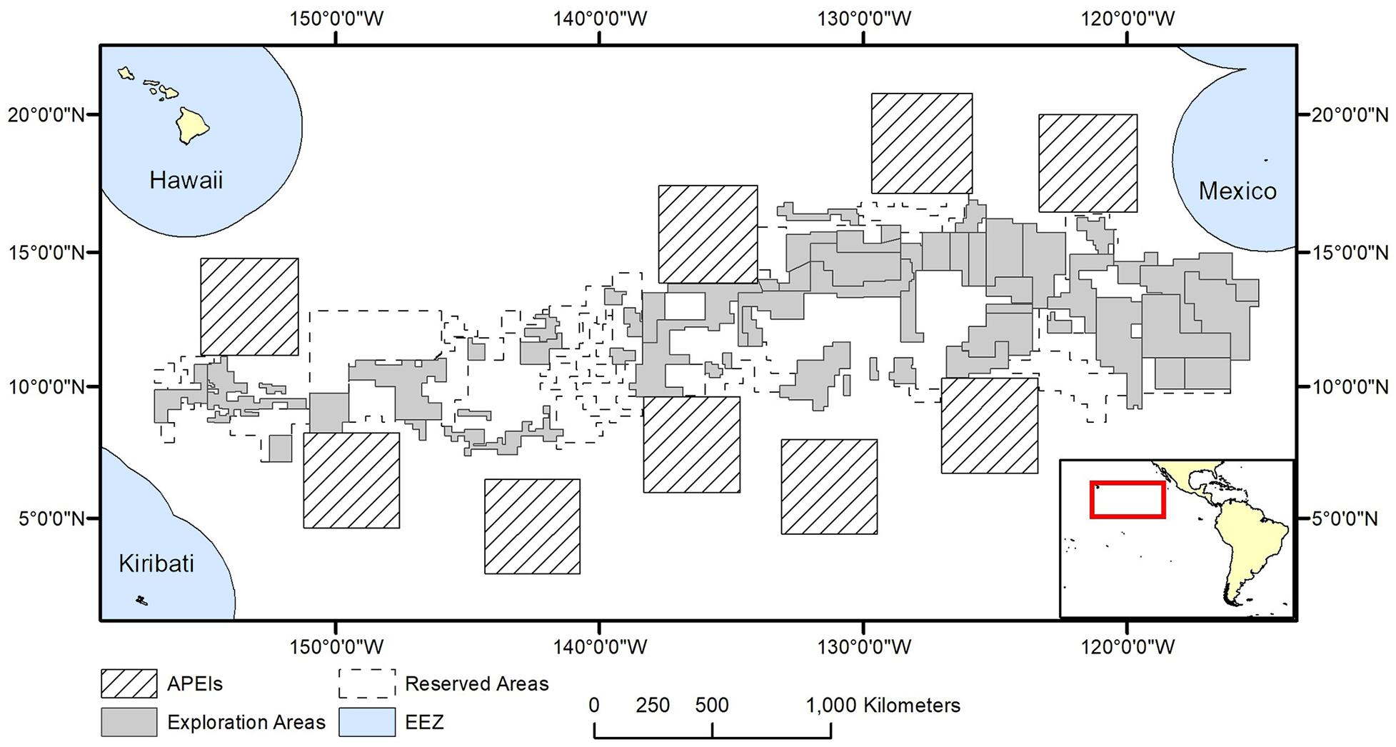
Figure 1. Polymetallic nodule exploration areas in the Clarion-Clipperton Fracture Zone, showing contractor exploration areas, reserved areas and Areas of Particular Environmental Interest (APEls).

Habitat Classification

We have used a two-step process to classify environmental surrogates in the CCZ. First, each environmental variable (or class of variables) was clustered (using a k-medoids, non-hierarchical clustering algorithm) to identify areas with different environmental conditions. Then, the outputs of the clustering for each environmental variable (or class of variables) were combined to give a final habitat classification.

Variable Selection

Environmental variables were selected for the classification based on evidence of key drivers of biophysical and ecological patterns and processes in the CCZ and the availability of those variables as continuous datasets across the region.

The variables used in this study were topography, POC flux to the seafloor and nodule abundance. While other variables may contribute to ecological patterns and processes in the CCZ, the selected variables are the most important variables (of those available) that have the strongest influences on biological communities in this area, as considered by an expert workshop on deep CCZ biodiversity (International Seabed Authority, 2020). It was expected that these drivers would be correlated with other parameters that were not included but may also influence species distributions. Although water-mass structure can be an important factor in determining the distribution of organisms in some marine environments (Tyler and Zibrowius, 1992; Howell et al., 2002; Miller et al., 2011), and has been used in global biogeographic classifications (e.g., Watling et al., 2013) to gain insight into species connectivity from transport and mixing processes, water-mass variables were not included because variations in water-mass structure (e.g., in temperature, salinity, dissolved oxygen concentration) are very small at the abyssal seafloor in the CCZ, and there is no evidence that water-mass structure drives differences in faunal communities across this area.

Topography

Depth and topography play an important role in determining species distributions in the deep sea, with species showing preference for certain depth ranges and topographic conditions (Rowe and Menzies, 1969; Hecker, 1990; Rice et al., 1990). In abyssal regions, and specifically the CCZ, where there are seamounts, troughs and ridges, topographic variation has been shown to influence biological communities (Durden et al., 2015; Stefanoudis et al., 2016; Leitner et al., 2017; Simon-Lledó et al., 2019a).

Although depth is a crucial factor in determining species distribution, and depth data is readily available, this parameter acts as an indirect surrogate for those variables actually driving distributions, such as temperature, pressure, oxygen, water mass structure and food supply (Evans et al., 2015), and was therefore excluded from this study. Rather, the underlying variables driving distributions were included (see below) and derivatives of bathymetry were used to represent topographic features of the region: slope, broad-scale bathymetric position index (BBPI) and fine-scale bathymetric position index (FBPI).

Slope is a first-order derivative of bathymetry, and acts as a surrogate for local hydrodynamics (Guinan et al., 2009), as benthic currents are steered by seafloor terrain and current velocities can be enhanced along steep slopes (Genin et al., 1986). Such currents affect sediment particle size distribution and drive the near-seabed horizontal flux of food particles to influence the abundance and community structure of benthic assemblages, particularly suspensions feeders (Gage and Tyler, 1996; Durden et al., 2015).

Bathymetric position index (BPI) is a second-order derivative of bathymetry, and gives the relative elevation of a point in relation to the overall landscape (Lundblad et al., 2006). Positive values indicate features rising above the surrounding terrain (e.g., peaks and crests), while negative values indicate depressions such as valleys and troughs. Areas with constant slope or flat areas are represented by near-zero values. BPI acts as a surrogate for various environmental factors that affect species distributions, such as exposure to current, current speed and sedimentation, without confounding the effects of other variables (e.g., temperature and salinity) as depth does (Evans et al., 2015).

Topographic variables were derived from the publically available General Bathymetric Chart of the Oceans (GEBCO) 2014 gridded bathymetry data¹. All variables were generated in ArcMap 10.4 using the Benthic Terrain Modeler extension (Wright et al., 2005) (Figure 2). Slope is determined as the largest change in elevation between a cell and its 8 nearest neighbors. BPI was derived at both broad and fine scale (called BBPI and FBPI, respectively), to capture topographic features at different scales across the region. BBPI was derived with an inner radius of 1 and an outer radius of 100, with a scale factor of 100 km. This broad-scale layer identified large geomorphological units, such as abyssal plains, steps and troughs. FBPI was derived with an inner radius of 1 and an outer radius of 10, with a scale factor of 10 km. This finer scale layer identified smaller “megahabitats,” i.e., features on the scale of kilometers to tens of kilometers, as defined in Greene et al. (1999). These features included seamounts, abyssal hills, canyons, plateaus, large banks and terraces.

FIGURE 2

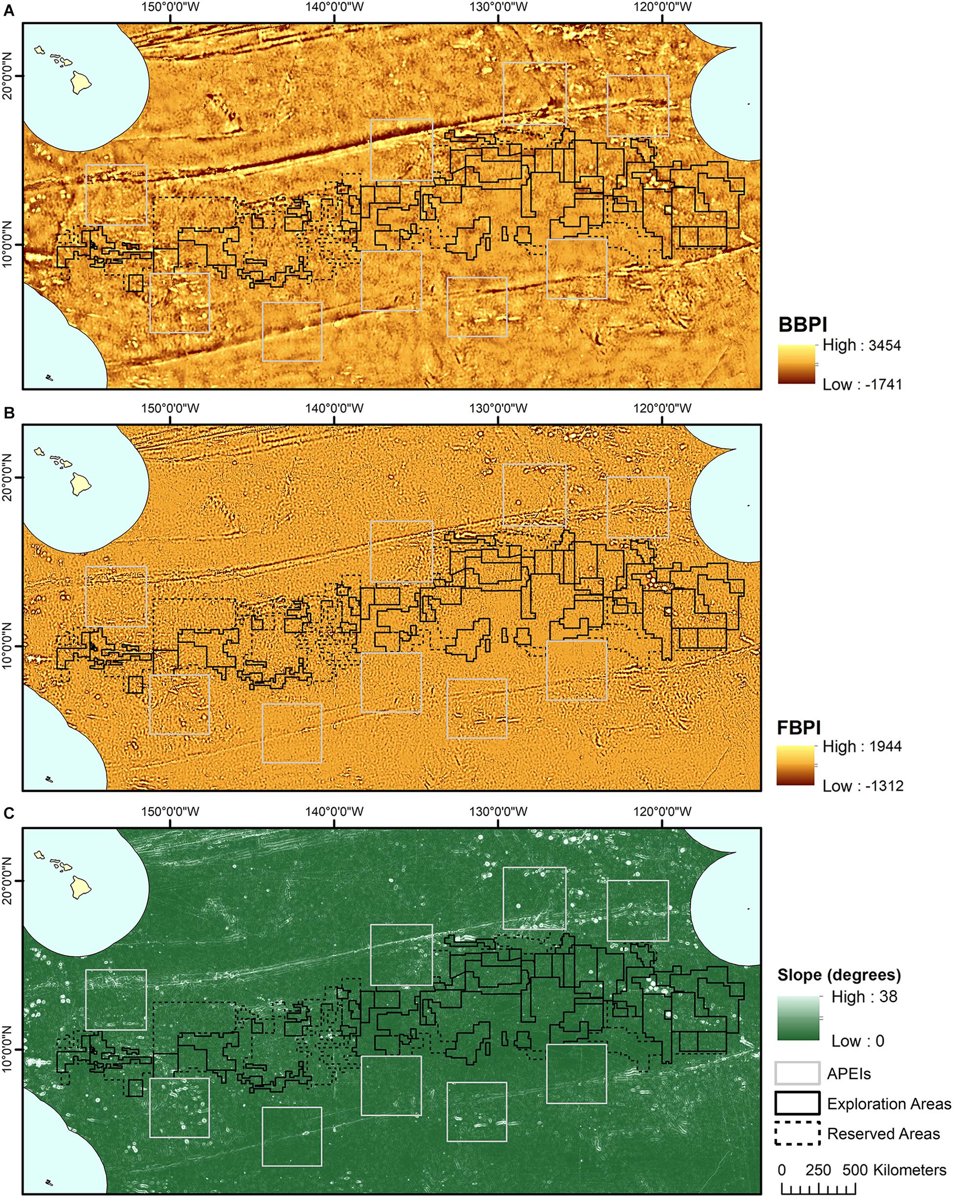
Figure 2. Topographic variable layers used in initial clustering, (A) broad-scale bathymetric position index (BBPI), (B) fine-scale bathymetric position index (FBPI), and (C) slope, derived from GEBCO 2014 bathymetry data and interpolated to 1 km² resolution. Land masses are shown in cream as labeled in Figure 1, surrounded by EEZs in pale blue.

Particulate organic carbon flux

Food availability plays arguably the most important role in determining the distribution of organisms at abyssal depths (Cartes and Sarda, 1993; Smith et al., 1997, 2008; Levin et al., 2001; Gooday, 2002; Ruhl and Smith, 2004; Wei et al., 2011; Woolley et al., 2016). In this food-poor environment, organisms are dependent on detrital matter in the form of POC sinking from surface waters to the seafloor (POC flux), except for cases of large organic food falls and chemosynthetic habitats (Turner, 1973; Gooday et al., 1990; Van Dover, 2000; Smith and Baco, 2003). As a result, community structure, function and diversity, life history patterns, body size, and feeding type, amongst others, are all strongly dependent on POC flux to the seafloor (Smith et al., 2008).

In the CCZ there is a strong gradient in POC flux, decreasing from east to west, and from south to north (Smith et al., 1997; Pennington et al., 2006; Lutz et al., 2007). This gradient has been linked to differences in faunal communities (e.g., Smith et al., 1997, 2008; Veillette et al., 2007; Vanreusel et al., 2016; Bonifácio et al., 2020).

Estimates for POC flux to the seafloor in the CCZ were obtained from a global model produced by Lutz et al. (2007), based on water depth and seasonal variability in remote-sensed net primary productivity data between 1997 and 2004. These estimates were interpolated to a 1 km² resolution across the model domain using kriging (Figure 3).

FIGURE 3

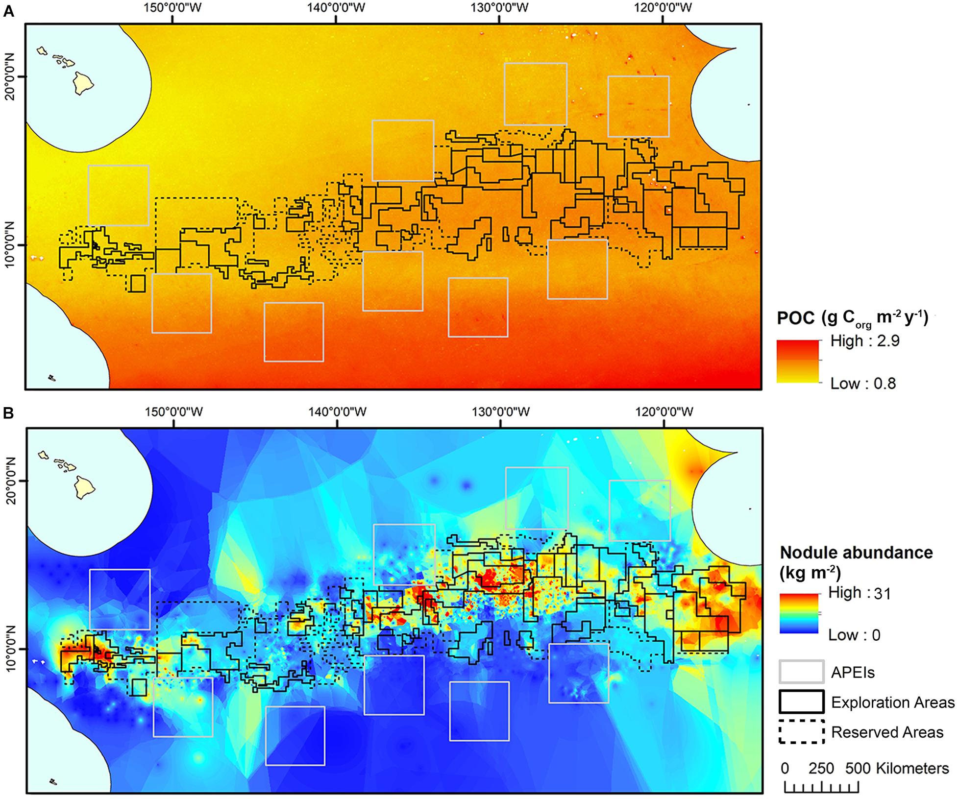
Figure 3. (A) POC flux at the seafloor modeled across the CCZ by Lutz et al. (2007), interpolated to 1 km² resolution and used in initial clustering and (B) Nodule abundance modeled across the CCZ (see International Seabed Authority, 2010), interpolated to 1 km² resolution and used in initial clustering.

Substrate

The use of substrate as a surrogate to represent biological diversity in deep-sea habitat classifications is well established (Howell, 2010). Although there is no global map of seabed substrate, polymetallic nodules provide most of the hard substrate in the CCZ and their abundance thus provides a proxy for hard substrate across the region.

Nodules provide habitat for encrusting and epifaunal species that depend on hard surfaces for attachment and feeding (e.g., Dugolinsky et al., 1977; Gooday et al., 2015; Amon et al., 2016), and support a range of fauna in nodule crevices (Thiel et al., 1993; Bussau et al., 1995). The increased habitat heterogeneity provided by nodules has been suggested to influence faunal standing stocks and enhance biodiversity compared to nodule-free abyssal environments (Amon et al., 2016; Vanreusel et al., 2016; Gooday et al., 2017), and a recent study provided the first quantified evidence that variations in nodule cover in the CCZ influence faunal standing stock, faunal composition, functional group composition, the distribution of individual species and some biodiversity attributes (Simon-Lledó et al., 2019b).

Modeled estimates of nodule abundance across the CCZ region were obtained from an existing geological model of nodule deposits in the CCZ, produced as part of an ISA technical study (see International Seabed Authority, 2010) (Figure 3). This model was developed by a group of technical experts (not the authors of the current study) and used both publicly available and proprietary data (i.e., data belonging to contractors with exploration contracts), primarily from the central CCZ. Five datasets comprising 61,583 stations provided data on nodule abundance (weight of nodules per unit of seafloor area in kg.m^–2), mainly from free-fall grab samples and some box cores. In order to protect proprietary concerns, data were grouped at one–tenth of a degree resolution, and then interpolated and extrapolated to estimate nodule abundance across the CCZ in areas not covered by available data. For more information on the nodule abundance data used in this study see International Seabed Authority (2010).

Although this data layer does not reflect the high variability in nodule abundance on small spatial scales (Peukert et al., 2018), it is the best available data, and the classification makes the assumption that broad patterns in nodule abundance are more important than smaller scale heterogeneity in driving regional patterns in species distributions.

Pre-processing and Cluster Analysis

All environmental variables were interpolated to 1 km² and projected in WGS 1984 PDC Mercator, an equal-area projection suitable for use in the Pacific Ocean. An equal-area projection was used so that estimates of the area of each habitat class identified through the classification could be calculated. Mercator is also a popular projection for navigation as it uses straight-line segments that represent true bearings, and outputs from the classification could therefore be used to support the implementation of spatial management measures.

We used an unsupervised, non-hierarchical clustering algorithm called Clustering Large Applications (CLARA) (Kaufman and Rousseeuw, 1990). CLARA is a k-medoids technique that clusters data points around the medoids (similar in concept to centroids, but always members of the data set) and is appropriate for use with large datasets.

A separate CLARA analysis was used to carry out unsupervised clustering on each class of variable: (1) topographic variables (FBPI, BBPI and slope), (2) POC flux, and (3) nodule abundance. This step allowed the combination of multiple topographic variables to produce a single layer representing the topographic variable class, and thus providing equal weighting to all classes of variables (topography, POC flux and nodule abundance) when combined in the final classification (see below). Based on the current level of knowledge of the drivers of species distributions in the CCZ, and in abyssal plains in general, it is not yet possible to confer weighting to classes of variables. An alternative approach would be to use all five environmental variables in a single clustering step. However, we felt this was inappropriate as this would give greater weighting to the role of topography in the resulting classification output simply due to the use of more topographic environmental variables. Our approach ensured topography, POC flux to depth, and nodule abundance contributed equally to the final output.

Pre-processing and clustering was carried out in ArcGIS 10.4 and R 3.3.1 (R Core Team, 2017), within the Rstudio environment (RStudio Team, 2015), using the “fpc” package and CLARA function (Hennig, 2015). As the focus of this study is on the deep sea in international waters, the EEZs of countries were excluded from the analysis. Prior to clustering, all variables were normalized to have equal variance and a common scale of 0–1. CLARA requires the user to define the number of clusters the dataset should be split into, and for each analysis clustering was therefore run a number of times, using a different number of clusters in each iteration, in order to identify the most parsimonious number of clusters (see below). Reproducible code for the cluster analysis is available in Supplementary Materials.

Evaluation of Clusters

In order to evaluate clustering and select appropriate numbers of clusters, two indices were used: average silhouette width (ASW) and the Calinski-Harabasz index (CH) (both built into the R CLARA function). The silhouette width of an object is a measure of how similar it is to its own cluster, compared to other clusters. ASW gives the average of all silhouette widths in a dataset, with the output being one value representing the overall silhouette width for the whole cluster analysis. This method compares the ASW of clustering iterations with different numbers of clusters, and the optimum number of clusters is the one with the highest ASW (Kaufman and Rousseeuw, 1990). The CH index assesses clustering by comparing the average between- and within-cluster sum of squares (Calinski and Harabasz, 1974). Here again the best clustering is the iteration with the largest CH value. Expert judgment based on literature and unpublished data was also used to further refine the final choice of number of clusters.

Finalization of Classification

Once the number of clusters was finalized for each variable class (topography, POC flux and nodule abundance), the three layers were combined in ArcGIS 10.4 using the “Combine” tool to produce the final habitat classification. This was a raster layer, with each cell assigned a habitat class representing a different set of environmental conditions, showing habitat heterogeneity across the region. As the modeled nodule layer displayed artifacts toward the periphery of the model domain, and certain combinations of environmental conditions were improbable (discussed below), a manual assessment of the confidence level of each habitat class was also carried out.

APEI Representativity

In order to test the habitat representativity of the current APEI network, the proportions of each habitat class from the classification located in the APEls, exploration and/or reserved areas, and unmanaged areas of the CCZ EMP area were calculated. Under the CBD, the current target for global representation of coastal and marine areas is 10% of target regions by 2020 (Convention on Biological Diversity, 2010), with a more ambitious target of 30% advocated at the 2003 and 2014 World Parks Congress (International Union for Conservation of Nature, 2005, 2014). In addition, Foster et al. (2013) calculated that between 30 and 40% was needed to conserve 75% of bathyal deep-sea species. Proportions of each habitat class in the current APEI network were compared to these targets. In addition, the number of APEIs within which each habitat class occurs was also calculated. Habitat classes with lower confidence were included in these calculations, and where reported are accompanied by the caveat that these should be treated with caution. All analyses were carried out in ArcGIS 10.6.

Results

Initial Clustering

In most cases, the clustering iteration with the highest ASW and CH values were chosen for the habitat classification, and this decision was supported by literature and expert review (Table 1). Topographic variables showed the best clustering with two groups. The two topographic clusters distinguished areas that were relatively flat (0 – 6 degrees slope), with small topographic features, from those that were more sloped (0 – 38 degrees), with more prominent peaks and troughs (Table 2 and Figure 4A).

TABLE 1

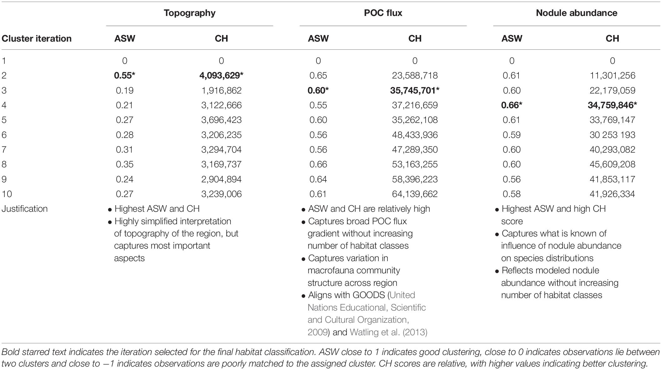
Table 1. Average silhouette width (ASW) and Calinski-Harabasz index (CH) for CLARA clustering iterations with 1–10 clusters for each class of environmental variables.

TABLE 2

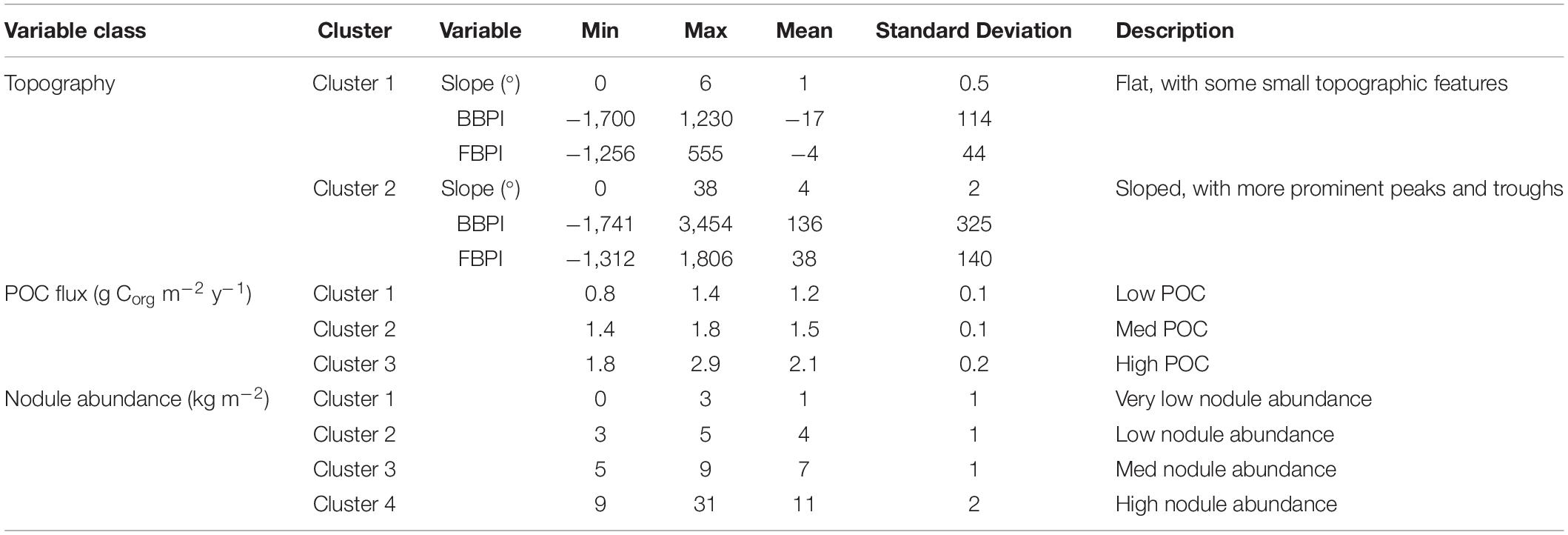
Table 2. Properties of clusters selected for the final habitat classification, produced through CLARA clustering of environmental surrogates.

FIGURE 4

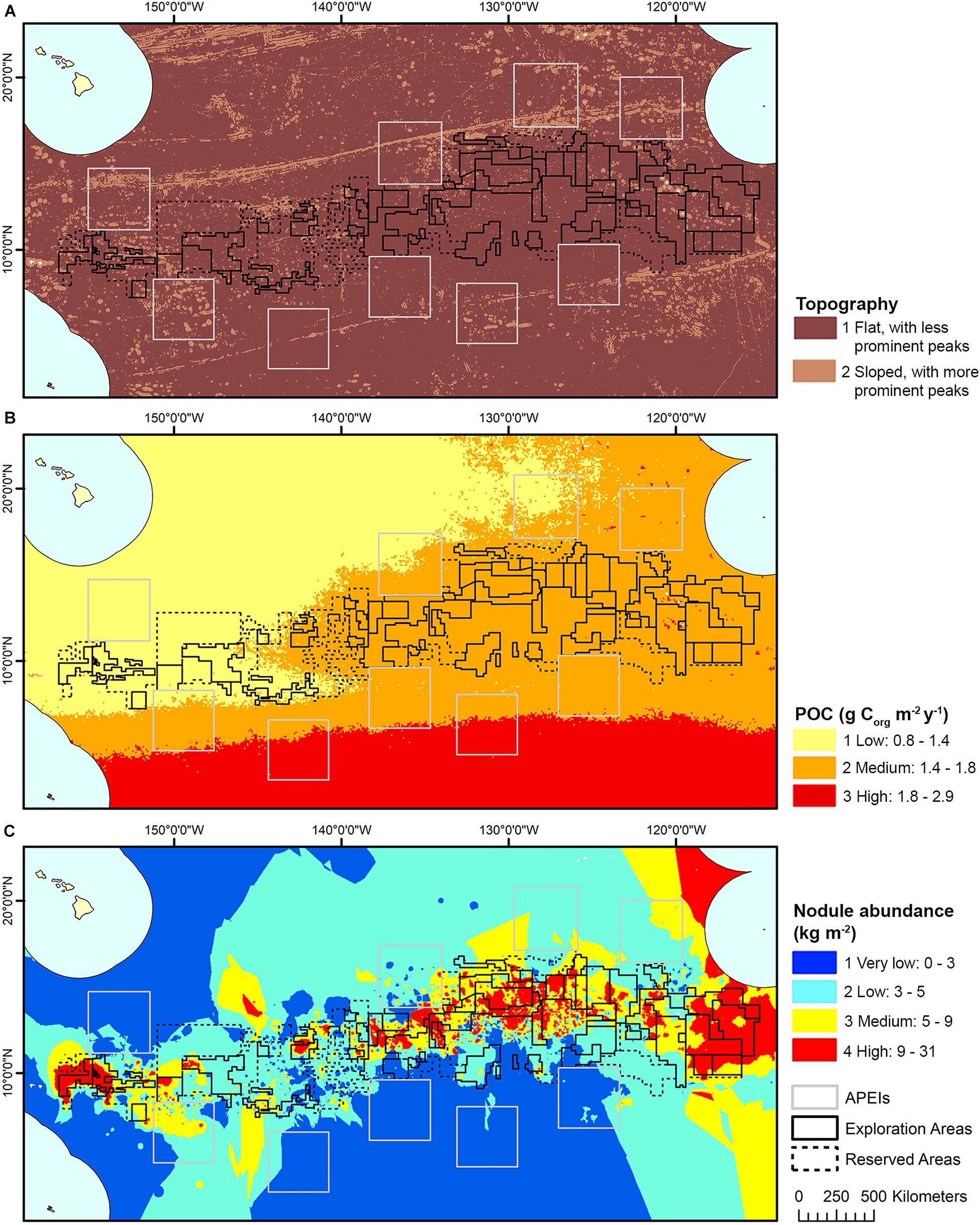
Figure 4. Outputs of initial CLARA clustering on variable classes to represent (A) topography, (B) seafloor POC flux, and (C) nodule abundance in the CCZ region, used in the final habitat classification.

Seafloor POC flux clustered best into 8 and 10 groups (based on ASW and CH indices, respectively), and this highlighted what is known in the literature of trends in POC flux across the region, with a gradient of high to low POC flux from east to west and south to north (Lutz et al., 2007). However, ASW and CH indices also performed well with just 3 clusters, and in order to simplify the classification this smaller number of clusters was chosen (Table 2 and Figure 4B). This clustering captured the broad pattern of seafloor POC flux across the region and supported variation in macrofauna community structure observed in the CCZ, from east to west and south to north (e.g., Glover et al., 2002; Smith et al., 2008; Bonifácio et al., 2020). It also aligned with the north-south split in biogeographic provinces in the CCZ identified by the GOODS (United Nations Educational, Scientific and Cultural Organization, 2009) and Watling et al. (2013) classifications in this region, which were both driven primarily by differences in POC flux.

Nodule abundance showed the best clustering with 4 and 8 groups (based on ASW and CH respectively). Given the current state of knowledge on the influence of nodule abundance on species distributions and the high CH value for 4 groups, 4 clusters were chosen for the final classification (Table 2 and Figure 4C). These four levels allow discrimination between areas of high and low nodule density at less than 50% nodule cover and for which there is ample evidence of difference in community composition and densities (Amon et al., 2016; Vanreusel et al., 2016; Simon-Lledó et al., 2019b), but also allows for the uncertainty in what happens to reported relationships at nodules densities > 50% and for which there are no published studies. Areas of medium to high nodule abundance were concentrated in the central CCZ, with some medium to high nodule abundance areas also predicted in the north- and southeast, as well as the southwest. Predictions of high nodule abundance to the northeast reflect favorable conditions for finding undiscovered nodule deposits, while projections of medium nodule abundance in the southeast and -west may be extrapolation artifacts in the input modeled nodule data, as seafloor POC fluxes in these areas are incompatible with the occurrence of nodules (International Seabed Authority, 2010).

Final Habitat Classification

The final classification produced by combining layers of clustered environmental variables proposes 24 habitat classes (Figure 5). Each habitat class represents a different set of environmental conditions (Table 3), and is assumed to support a distinct biological community. It is worth noting that the boundaries between adjacent habitat classes will include zones of transition and will not be as abrupt as is reflected by the classification.

FIGURE 5

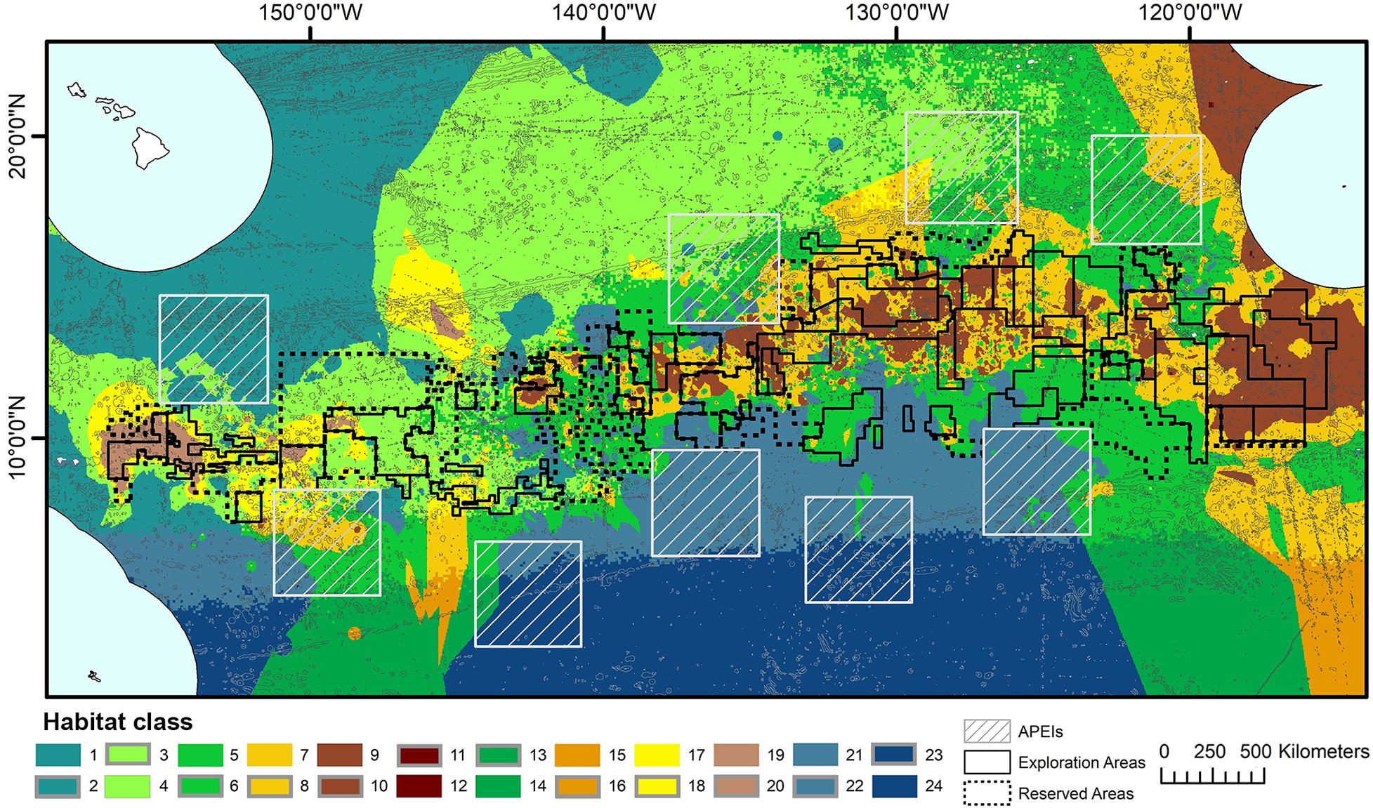
Figure 5. Final 24 habitat classes produced by combining layers of clustered environmental variables. Habitat classes with high nodule abundance are shown in shades of brown, medium nodule abundance in orange/yellow, low nodule abundance in green and very low nodule abundance in blue. Within each nodule abundance group (i.e., very low, low, medium or high), habitat classes with different POC flux to the seafloor are identified by shading (i.e., darkest brown = high nodule abundance, high POC flux; lightest brown = high nodule abundance, low POC flux). Habitat classes with sloping topography are then identified by gray outlines. For example, habitat classes 1 and 2 have the same POC flux and nodule abundance conditions, but differ in topography. Habitat class 1 has very low nodule abundance, low POC flux and is flat, while habitat class 2 has very low nodule abundance, low POC flux and is more sloped.

TABLE 3

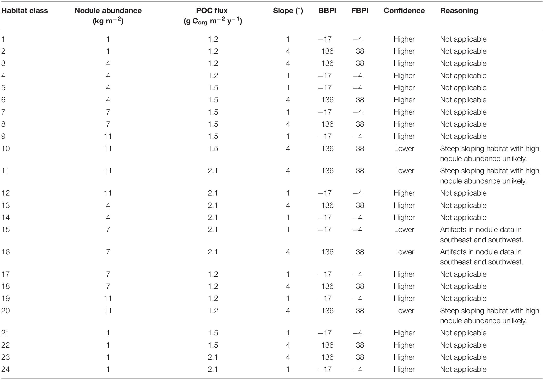
Table 3. Environmental characteristics (mean values) of each habitat class, indicating confidence with which the class should be treated.

Habitat classes in the east are characterized by medium to high seafloor POC flux, in the north- and southeast respectively. In the west, habitat classes are mainly areas of low POC flux, with medium to high POC flux in the southwest. Habitat classes with medium to high nodule abundance are concentrated in the central CCZ, bounded by the Clarion and Clipperton fracture zones and overlapping with exploration contracts and reserved areas. The periphery largely contains habitat classes with low and very low nodule abundance, although some medium and high nodule abundance habitat classes are also predicted in areas to the southwest, southeast and northeast of the central CCZ (but see caveats below).

Habitat classes with high nodule cover make up only 6.6% of the total area, which is otherwise dominated by low and very low nodule abundance (42 and 36% of the CCZ EMP area, respectively). The large habitat classes are also predominantly flat abyssal plain, with pockets of smaller classes distinguished by sloping topographic features like seamounts, peaks and troughs. In fact, 89% of the area is composed of habitat classes that are flat or of constant slope with small topographic features, while only 11% consist of varying slope characteristic of larger peaks and troughs.

Based on this classification, the CCZ EMP area appears to be dominated by several very large habitat classes, with many smaller pockets of different habitat classes spread across the area (Figures 5–7). The three most abundant habitat classes identified (numbers 4, 5, and 24, each with >1.4 million km², Table 4) are flat with some small topographic features, low to high POC flux to the seafloor, and low to very low nodule abundance. Two of these three largest habitat classes occur mainly on the periphery of the central CCZ, to the north and south, while the third occurs across parts of the central CCZ and to the northeast. In total, these habitat classes make up 44% of the EMP area. In fact, out of 24 habitat classes, the largest five form over 60% of the modeled area. These five largest habitat classes (1, 4, 5, 7, and 24) differ in terms of the level of POC input and nodule cover, but are all characterized by the same topographic conditions, i.e., flat or constant slope with some small topographic peaks and depressions.

FIGURE 6

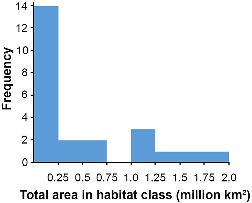
Figure 6. Number of habitat classes of different total areas.

FIGURE 7

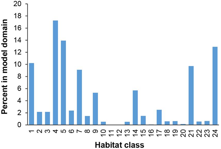
Figure 7. Percentage of model domain within each habitat class.

TABLE 4

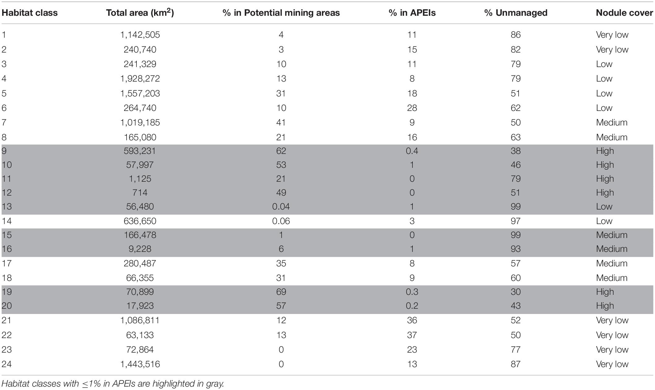
Table 4. Total extent of each habitat class, and percent located in potential mining areas (exploration and/or reserved areas), Areas of Particular Environmental Interest (APEI), and unmanaged areas as of June 2019.

The three smallest habitat classes in total area (classes 11, 12, and 16) all contain medium to high nodule abundance and are found predominantly to the east or in the southwest.

Confidence levels assigned to each habitat class reflect the confidence with which the class should be treated (Table 3). As noted above, projections of medium nodule abundance to the southeast and -west of the CCZ may be extrapolation artifacts in the input modeled nodule data (International Seabed Authority, 2010), and habitat classes in these areas (i.e., classes 15 and 16) should thus be treated with caution. In addition, certain combinations of environmental conditions are deemed to be improbable. Habitat classes with high nodule abundance and more sloped topographic features (i.e., classes 10, 11, and 20) may result from the broad-scale nodule abundance input data not reflecting small-scale heterogeneity in nodule abundance with topographic features. Nodules are not known to occur on the steep flanks of seamounts, and therefore some areas with sloped topography and high nodule abundance may not actually have high nodule abundance. However, the sloped topography cluster with more prominent peaks and troughs does not identify only seamounts, but also more gently sloping topographic features that may support nodules. Slope in this cluster ranges from 0 to 38 degrees, and nodules may be found in areas of intermediate slope, up to 15 degrees (e.g., see Sharma and Kodagali, 1993; Yamazaki and Sharma, 1998; Bu et al., 2003; Kuhn et al., 2012). We therefore advise that classes with sloped topography and high nodule abundance are treated with some caution, as parts of these habitats may be improbable. The following results should be considered with the aforementioned caveats in mind.

APEI Representativity

An assessment of the habitat representativity of the CCZ APEI network shows that 21 habitat classes of a total of 24 are included in the APEls, with 22 habitat classes occurring in exploration and/or reserved areas (Table 4). In the following we present results for the exploration and reserved areas combined. These are referred to as “potential mining areas,” since both are ultimately intended for potential mining activities. They are up-to-date with all contracts awarded as of June 2019.

In the current APEI network, 14 habitat classes (nearly 60% of the total number of habitat classes in the area) have less than 10% of their area represented within APEIs, and 10 of these are represented by less than 5% (Figure 8). These 14 habitat classes have a range of environmental conditions including all topographic and POC flux conditions, and low to high nodule abundance levels. Seven habitat classes are represented by less than 1% (classes 9, 10, 11, 12, 13, 15, 16, 19, and 20), and of these, three receive no protection in the APEI network at all (classes 11, 12, and 15). Those habitat classes with greater than 0% but less than 1% representation in the APEls are fairly large, ranging in total size from 9,000 to 593,000 km², and are generally located in large patches in the central CCZ. Those habitat classes with no protection at all have medium to high nodule abundance, high POC flux and variable topographic conditions. They include two smaller classes (numbers 11 and 12, <2,000 km² total area), and one larger class (number 15, >160,000 km²). Habitat classes 11 and 12 are found in small pockets focused around topographic features with apparent high nodule abundance, and class 15 occurs in larger areas of medium nodule abundance in the southeast and southwest. Habitat classes 15 and 11 should be treated with caution, as above (Table 3). At the more ambitious World Park’s Congress conservation target of 30% protection, which is at the lower end of what is required to conserve 75% of bathyal species (Foster et al., 2013), just two habitat classes are found to be adequately represented in the current APEI network. This means that 92% (22 classes) are not adequately protected at the 30% level.

FIGURE 8

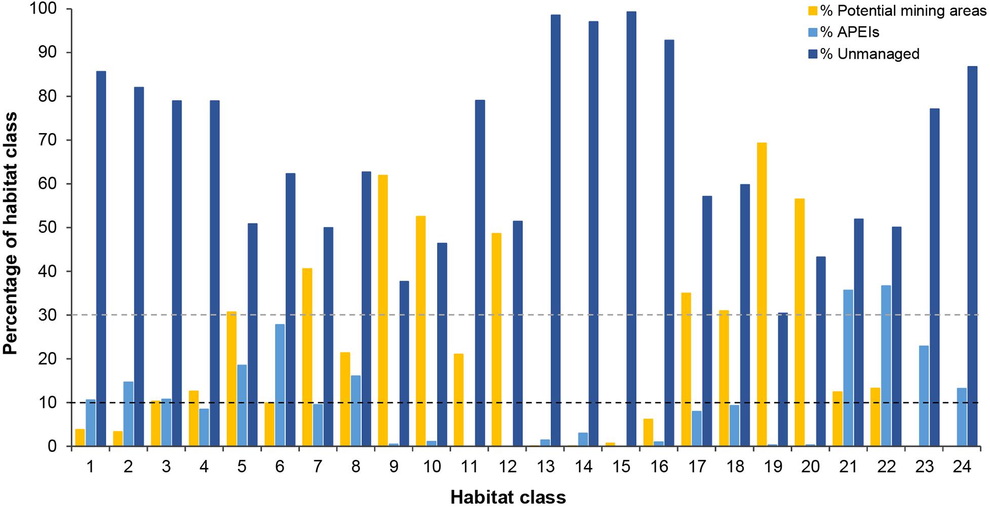
Figure 8. Percentage of the total area of each habitat class occurring in APEls, potential mining areas (exploration contracts and/or reserved areas) and unmanaged areas. Dashed lines represent conservation targets|

Of the 14 habitat classes with < 10% representation in the APEls, 10 have > 10% of their total area in potential mining areas (Table 4 and Figure 8). Habitat classes 9, 10, 19, and 20 have 0% or nearly 0% representation in APEls and a large proportion (50% to ∼ 70%) of their total extent located in exploration and/or reserved areas. These are all habitat classes with high nodule abundance located predominantly in the central CCZ (Figure 4C), and range in size from 17,000 km² to ∼ 600,000 km². These habitat classes also have a fairly high proportion of their area in currently unmanaged areas, which could be considered for spatial management. Two other habitat classes (11 and 12) are also unrepresented in APEls, with a high proportion of their area in high-nodule-abundance potential mining areas; and these classes are small in total extent, focused around topographic features with high POC (Figure 7 and Table 4). Of the habitat classes with <30% representation in the APEls, 13 have >10% of their total area located within potential mining areas, while 11 have >20%, and four have >50%.

Three habitat classes (13, 15, and 16) are represented by ≤1% in APEls and have a high proportion (>90%) of their total extent in unmanaged areas. These habitat classes are located in the southeast and southwest of the CCZ EMP area, in areas of low to medium nodule abundance, high POC flux and varying topographic conditions.

Finally, two habitat classes (classes 23 and 24) are not found in potential mining areas, but are represented in the APEI network. Both habitat classes occur to the south of the central exploration and reserved areas, and have very low nodule abundance (with other conditions varying). Four habitat classes (numbers 1, 2, 23, and 24) have > 10% (but <25%) of their total area in APEls, and less than 5% of their area in potential mining areas. These habitat classes range in total area from 72,800 km² to 1,443,000 km² and are located in the northwest, in the south in central to western areas, and in smaller pockets in the central CCZ. These habitat classes also all have very low nodule cover.

In terms of replication of habitat classes within the APEI network, several classes (9, 10, 11, 12, 15, 16, 19, and 20) were found to occur in either no APEIs, or only one or two (Figure 9).

FIGURE 9

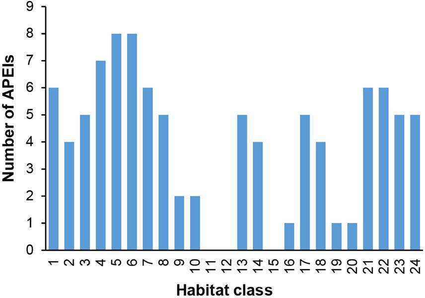
Figure 9. Number of APEIs within which each habitat class is represented.

Discussion

Comparison With Global Classifications

Our final habitat classification yields 24 benthic habitat classes that are assumed to support distinct faunal communities. Each of these habitat classes represents a different set of environmental conditions, based on the topographic features of the area, POC flux to the seafloor, and the abundance of nodules. According to this classification, the CCZ is dominated by several large, flat habitat classes with constant slope and relatively small topographic features, with many smaller pockets of different habitat classes interspersed across the region. Areas of high nodule abundance are predominantly located in the central CCZ, with a large patch of high nodule abundance in the northeast (Figure 5).

No similar, regional-scale habitat classifications have been carried out in the CCZ region, but the current classification can be compared with other global efforts that cover the region. These include the GOODS classification United Nations Educational, Scientific and Cultural Organization (2009), Watling et al. (2013), Harris and Whiteway (2009) and Sayre et al. (2017). These are all larger scale, global classifications that describe large-scale units, in some cases based on biogeography (ecosystems with shared evolutionary processes and a suite of endemic species). The scale of the classes in these classifications is not suitable for use in regional environmental management, nevertheless, they provide a broad context for this habitat classification. Both GOODS and Watling et al. (2013) proposed two biogeographic provinces overlapping the CCZ, split in a north-south direction, with the boundaries for these driven primarily by differences in POC flux across the region. This split is captured in the current classification, which identifies habitat classes falling within areas of different POC flux, mainly in a latitudinal direction. Although a similar pattern is observed in the pelagic portions of the classification by Sayre et al. (2017), at the benthic level, the CCZ falls within a single Ecological Marine Unit. The classification produced by Harris and Whiteway (2009), on the other hand, is a somewhat finer scale, and splits the equatorial Pacific longitudinally, proposing different seascapes in the east and west, reflecting two different water masses identified in the region. Although water-mass structure may be an important factor in determining species distributions in other ocean basins (Howell et al., 2002), and has been used in previous global classifications (e.g., Watling et al., 2013), this variable was not included in the current study because there is little ecologically significant variation in water-mass characteristics across the CCZ (Watling et al., 2013), and there is no evidence that species distributions are driven by water-mass structure in this region.

It is worth noting that the underlying environmental models used to build the classification contain known, but unquantified, error. For example, the nodule abundance layer was produced using data primarily located within the central CCZ, which was then extrapolated outwards to predict nodule abundance in peripheral areas. This results in some artifacts, as previously mentioned. All layers were produced to reflect broad-scale variability only, and thus the constructed habitat classification is also only able to reflect broad-scale variability. In addition, limitations to the classification approach, including missing an important explanatory variable, not weighting input variables, issues with scale and selection of the number of clusters, and generation of clusters that represent environmental conditions that are unlikely to occur, may have impacted the model outputs. Most of these issues result from insufficient knowledge of the drivers of faunal communities in environments like the CCZ, and a general lack of both biological and environmental data. Acknowledging these potential shortcomings, this approach still has an important role to play in spatial planning, and makes use of best available data.

APEI Representativity

Representativity Assessment

Habitat representativity is a well-accepted requirement for MPA design (OSPAR Commission, 2006; Convention on Biological Diversity, 2009; O’Leary et al., 2012) and is one of the principal criteria for an MPA network to be considered ecologically coherent (Ardron, 2008; OSPAR Commission, 2010). The current CCZ APEI network does not fully meet representativity requirements, based on either the CBD conservation target of protection of 10% of the area of all habitat types (Convention on Biological Diversity, 2010), or the larger World Park’s Congress target of 30% (International Union for Conservation of Nature, 2005, 2014). Recognizing the caveats previously mentioned, a large proportion of habitat classes (over half) are represented in the protected area network by less than 10% of their total extent, with the vast majority represented by less than 30% of their area. However, because the total area of current APEIs covers only 24% of the CCZ EMP area, a 30% conservation target is not realistic without additional APEIs.

Many habitat classes are represented in APEIs by <1% of their area, and some (3) are absent from the APEI network completely. Among the least protected habitat classes, many occur in large areas with high nodule abundance distributed across the central CCZ; those receiving no protection are generally found in smaller pockets on the periphery in areas of medium to high nodule abundance. Some of these are very small habitat classes, which is of concern as smaller, less common habitats may require greater protection than large, widely distributed ones (Johnson et al., 2014). Habitat classes 11 and 12, for example, occur around specific seabed features and may require additional, targeted protection at a scale that is much smaller than the size of a full APEI. Although these habitat classes are unlikely to be mined due to their topographic characteristics, they may still be vulnerable to impacts from adjacent mining such as sediment plumes. It is important to remember the caveats around habitat class 11, stated in the results (and see Table 3).

Several of the habitat classes with low representation (below 1%) in APEls are found to have a large proportion of their total expanse (21 – 69%) in potential mining areas, and these are all habitat classes with high nodule abundance (numbers 9, 10, 11, 12, 19, and 20, although numbers 10, 11, and 20 should be treated with some caution, Table 3). The habitat heterogeneity introduced by nodules has been shown to increase megafauna abundance, with a positive relationship observed between megafauna abundance and nodule cover (Amon et al., 2016; Vanreusel et al., 2016; Simon-Lledó et al., 2019b). The link between increasing nodule cover and megafauna diversity is less clear, although no studies have yet been published from areas of high nodule abundance. Nonetheless, representation of all habitat types is required to support an ecologically coherent network of protected areas, including those with high nodule cover.

In addition, some habitat classes (13, 15, and 16) have a high proportion of their total extent in unmanaged areas, up to 99%, and <1% in APEIs. Considering habitat classes outside of exploration and reserved areas as “safe” is potentially unwise because these areas are not currently protected from mining. Exploration contracts in the CCZ are still being awarded (e.g., International Seabed Authority, 2017a), and some impacts from mining may well extend beyond the boundaries of contract areas (e.g., sediment plumes may be carried further afield by eddies, Aleynik et al., 2017). Further consideration of protection of these habitat classes may be required, although habitats 15 and 16 should be treated with caution (Table 3).

Finally, those habitat classes with low replication within the APEI network are also those with low representativity. All of these habitat classes have high proportions of their total extent within potential mining areas (numbers 9, 10, 11, 12, 19, and 20) or unmanaged areas (numbers 15 and 16).

Revisiting the CCZ APEI Network

This study suggests that to reach habitat representativity conservation targets, additional protection is required in the CCZ. Protected areas are currently largely located in the periphery of the central, high-nodule-abundance habitat classes, and thus fail to adequately protect these habitats. Such a network may fall short of representing all of the unique habitats and biodiversity of the area (O’Leary et al., 2012), and we suggest that additional APEl(s) are warranted in areas of high nodule abundance to augment protection.

When the APEI network was adopted by the ISA, some of the protected areas proposed by experts within the central CCZ were shifted to the periphery to avoid any overlaps with existing exploration and/or reserved areas, resulting in the current APEI distribution (International Seabed Authority, 2011; Wedding et al., 2013). New data on dispersal distances led to calls in 2016 for two additional APEls to the northwest and southeast of the current network, but not in the central nodule area (Figure 10) (International Seabed Authority, 2016). Although not formally quantified in this study, this habitat classification provides support for the establishment of these additional APEIs. Proposed APEI 10 would improve representation and replication of two habitat classes currently receiving little protection, but with high proportions of their total extent within potential mining areas (see locations of classes 19 and 20 in Figure 10), while proposed APEI 11 would slightly increase representation and replication of habitat classes 13, 15, 16. In addition, the classification identifies areas of habitat to the east of exploration contracts, south of the Mexican EEZ, that could provide protection of another two habitat classes currently poorly represented and replicated in APEIs, and with high representation in potential mining areas (see locations of classes 9 and 10 in Figure 10). Although not visible in Figure 10, pockets of habitat classes 11 and 12 are located in unmanaged areas to the northeast of APEI 6 and could be considered for future protection, acknowledging the caveats around class 11. The addition or modification of APEls based on improved knowledge of the CCZ was a key concept in the EMP (International Seabed Authority, 2011) and is consistent with an adaptive management approach that has been advocated by many for deep-sea mining (e.g., Jaeckel, 2016).

FIGURE 10

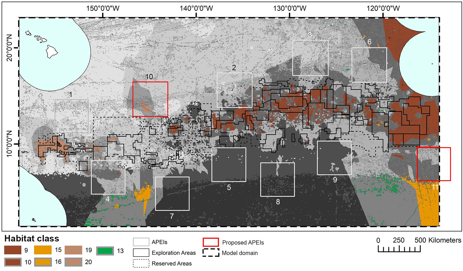
Figure 10. Distribution of habitat classes 9, 10, 13, 15, 16, 19, and 20 (with 0%, or nearly 0%, representation in APEls) in relation to two new Areas of Particular Environmental Interest (APEls) proposed for inclusion in the current Clarion-Clipperton Fracture Zone APEI network: numbers 10, to the northwest, and 11, to the southeast. Other habitat classes shown in grayscale.

Several habitat classes are located nearly entirely within the central CCZ, and conservation of these unique habitat classes would thus require protection measures that work around the existing mosaic of exploration and reserved areas, or utilize new space if areas are relinquished in future. These could take the form of smaller areas than a full APEI, although that would compromise the “buffer zone” that protects the core area of an APEI from possible impact from mining in an adjacent site.

The results from the Friday Harbor Deep CCZ Biodiversity Synthesis Workshop (International Seabed Authority, 2020), that includes a preliminary account of this habitat classification work, have been incorporated into the ongoing review in 2020 of the CCZ EMP by the Legal and Technical Commission of the ISA. The classification informs the discussion of how different habitat classes (and assumed benthic communities) are distributed within the current network of APEIs, where there are clear gaps and habitat classes that are not included, where habitat classes are only protected in a single APEI (no replication), and how the location of any new APEIs can maximize the inclusion of habitat classes that are poorly represented in the existing APEI network. This includes consideration of the distance between APEIs (and the suggested inclusion of APEIs 10 and 11 from 2016), as well as options for APEIs to the east of existing potential mining areas (considering adjacent EEZs) to protect representative nodule communities and/or inside the central nodule belt and mosaic of exploration contract areas and reserved areas.

Future Applications

This study provides an example of a classification method that can be used to support spatial planning in large, data-poor areas. Specifically, it could be used to inform the development of further EMPs [termed Regional Environmental Management Plans (REMPs)] in other regions targeted by seabed mining, which are required under the draft ISA Regulations for Exploitation (International Seabed Authority, 2019a) and encouraged by UNGA Resolution 68/70 (United Nations General Assembly, 2014, para. 51). The ISA has made progress in developing further REMPs (International Seabed Authority, 2019b) and we would recommend that the use of MSP in future REMP development frameworks be formalized. A proactive approach to designating protected areas in regions of interest for mining, but currently with low levels of activity, could help to avoid a scenario like the CCZ where certain habitat classes are largely contained within potential mining areas, and therefore could be more at risk. This would support a precautionary approach and would require a large collaboration between scientists, contractors, and the ISA. Although any network of protected areas will require revision as new scientific knowledge becomes available, the development of a benthic classification coupled with an APEI network proposal developed using MSP approaches would be a positive first step for areas of interest to mining, and would ensure that any future allocation of contract areas can balance both conservation and exploitation objectives.

In addition, under ISA recommendations to contractors on biological sampling to establish environmental baselines, contractors are advised to take samples of fauna that are representative of variability of habitats, bottom topography, depth, seabed and sediment characteristics, the water column and mineral resource being targeted [International Seabed Authority, 2019c, para.15 (d)]. A similar top–down benthic classification approach as used in this study could be applied at a finer scale within contractors’ exploration areas to support contractor’s sampling regime.

Conclusion

The habitat classification method applied in this study indicates the current APEI network in the CCZ does not fully represent all of the unique habitat classes found in this area, particularly those with high nodule abundance in the central CCZ. It is recommended that consideration should be given to additional APEls protecting areas of high nodule abundance, potentially to the east of existing contractor exploration areas, or smaller areas within the central CCZ. The habitat classification approach used here could be applied more widely to regional planning to ensure that such protected areas and networks are spatially coherent.

Data Availability Statement

The data analyzed in this study is subject to the following licenses/restrictions: Two datasets analyzed in this study do not belong to the authors. References to the reports and papers from which the data have come are provided in the manuscript. Requests to access these datasets should be directed to https://doi.org/10.1029/2006JC003706 (for POC flux data); and https://www.isa.org.jm/documents/geological-modelpolymetallic-nodule-deposits-clarion-clipperton-fracture-zone (for nodule abundance data).

Author Contributions

MA and KH obtained the funding for the study. KH and KM contributed to the conception and design. KM performed the classification, with technical input from AC and KH. All the authors contributed to the manuscript writing, read and approved the submitted version.

Conflict of Interest

The authors declare that the research was conducted in the absence of any commercial or financial relationships that could be construed as a potential conflict of interest.

The reviewer DV declared a past co-authorship with one of the authors CS to the handling editor.

Funding

This study first appeared in the Ph.D. thesis of KM (McQuaid, 2020). The authors would like to acknowledge UK Seabed Resources Ltd., for funding this research. The funder was not involved in the study design, collection, analysis, interpretation of data, the writing of this article or the decision to submit it for publication. CS and AG were supported by the G and B Moore Foundation. This is contribution no. 11198 from SOEST, University of Hawaii.

Acknowledgments

Thanks to Rebecca Ross and Nils Piechaud for technical support, and to participants of the Deep CCZ Biodiversity Synthesis Workshop for constructive feedback.

Supplementary Material

The Supplementary Material for this article can be found online at: https://www.frontiersin.org/articles/10.3389/fmars.2020.558860/full#supplementary-material

Footnotes

1. ^ https://www.gebco.net/

References

Aleynik, D., Inall, M. E., Dale, A., and Vink, A. (2017). Impact of remotely generated eddies on plume dispersion at abyssal mining sites in the Pacific. Sci. Rep. 7:16959. doi: 10.1038/s41598-017-16912-2

PubMed Abstract | CrossRef Full Text | Google Scholar

Altvater, S., Fletcher, R., and Passarello, C. (2019). “The need for marine spatial planning in areas beyond national jurisdiction,” in Maritime Spatial Planning, eds J. Zaucha and K. Gee (Cambridge: UN Environment World Conservation Monitoring Centre), 19.

Google Scholar

Amon, D. J., Ziegler, A. F., Dahlgren, T. G., Glover, A. G., Goineau, A., Gooday, A. J., et al. (2016). Insights into the abundance and diversity of abyssal megafauna in a polymetallic-nodule region in the eastern Clarion-Clipperton Zone. Sci. Rep. 6:30492. doi: 10.1038/srep30492

PubMed Abstract | CrossRef Full Text | Google Scholar

Ardron, J. (2008). Three initial OSPAR tests of ecological coherence: heuristics in a data-limited situation. ICES J. Mar. Sci. 65, 1527–1533. doi: 10.1093/icesjms/fsn111

CrossRef Full Text | Google Scholar

Ardron, J., Gjerde, K., Pullen, S., and Tilot, V. (2008). Marine spatial planning in the high seas. Mar. Policy 32, 832–839. doi: 10.1016/j.marpol.2008.03.018

CrossRef Full Text | Google Scholar

Bonifácio, P., Martínez Arbizu, P., and Menot, L. (2020). Alpha and beta diversity patterns of polychaete assemblages across the nodule province of the eastern Clarion-Clipperton Fracture Zone (equatorial Pacific). Biogeosciences 17, 865–886. doi: 10.5194/bg-17-865-2020

CrossRef Full Text | Google Scholar

Bu, W., Shi, X., Peng, J., and Qi, L. (2003). Geochemical characteristics of seamount ferromanganese nodules from mid-Pacific Ocean. Chinese Sci. Bull. 48, 98–105. doi: 10.1007/BF02900947

CrossRef Full Text | Google Scholar

Bussau, C., Schriever, G., and Thiel, H. (1995). Evaluation of abyssal metazoan meiofauna from a manganese nodule area of the eastern South Pacific. Vie Milieu 45, 39–48.

Google Scholar

Calinski, T., and Harabasz, J. (1974). A dendrite method for cluster analysis. Commun. Stat. 3, 1–27. doi: 10.1080/03610927408827101

CrossRef Full Text | Google Scholar

Cartes, J. E., and Sarda, F. (1993). Zonation of deep-sea decapod fauna in the Catalan Sea (Western Mediterranean). Mar. Ecol. Prog. Ser. 94, 27–34. doi: 10.3354/meps094027

CrossRef Full Text | Google Scholar

Chiba, S., Saito, H., Fletcher, R., Yogi, T., Kayo, M., Miyagi, S., et al. (2018). Human footprint in the abyss: 30 year records of deep-sea plastic debris. Mar. Policy 96, 204–212. doi: 10.1016/j.marpol.2018.03.022

CrossRef Full Text | Google Scholar

Clark, M. R., Watling, L., Rowden, A. A., Guinotte, J. M., and Smith, C. R. (2011). A global seamount classification to aid the scientific design of marine protected area networks. Ocean Coast. Manag. 54, 19–36. doi: 10.1016/j.ocecoaman.2010.10.006

CrossRef Full Text | Google Scholar

Connor, D. W., Allen, J. H., Golding, N., Howell, K. L., Lieberknecht, L. M., Northen, K. O., et al. (2004). The Marine Habitat Classification for Britain and Ireland Version 04.05. Peterborough: Joint Nature Conservation Committee, 49.

Google Scholar

Convention on Biological Diversity [CBD] (2009). Report of the Expert Workshop on Scientific and Technical Guidance on the Use of Biogeographic Classification Systems and Identification of Marine Areas Beyond National Jurisdiction in Need of Protection. Ottawa, ON: CBD.

Google Scholar

Convention on Biological Diversity [CBD] (2010). Report of the Tenth Meeting of the Conference of the Parties to the Convention on Biological Diversity. Nagoya: UNEP.

Google Scholar

Davies, C. E., Moss, D., and Hill, M. O. (2004). EUNIS Habitat Classification Revised 2004. Report to the European Topic Centre on Nature Protection and Biodiversity. Copenhagen: European Environment Agency, 307.

Google Scholar

De Santo, E. M. (2018). Implementation challenges of area-based management tools (ABMTs) for biodiversity beyond national jurisdiction (BBNJ). Mar. Policy 97, 34–43. doi: 10.1016/j.marpol.2018.08.034

CrossRef Full Text | Google Scholar

De Smet, B., Pape, E., Riehl, T., Bonifácio, P., Colson, L., and Vanreusel, A. (2017). The community structure of deep-sea macrofauna associated with polymetallic nodules in the eastern part of the Clarion-Clipperton Fracture Zone. Front. Mar. Sci. 4:1–14. doi: 10.3389/fmars.2017.00103

CrossRef Full Text | Google Scholar

Douglass, L. L., Turner, J., Grantham, H. S., Kaiser, S., Constable, A., Nicoll, R., et al. (2014). A hierarchical classification of benthic biodiversity and assessment of protected areas in the Southern Ocean. PLoS One 9:e100551. doi: 10.1371/journal.pone.0100551

PubMed Abstract | CrossRef Full Text | Google Scholar

Dudley, N. (2008). Guidelines for Applying Protected Area Management Categories. Gland: International Union for Conservation of Nature (IUCN), 86.

Google Scholar

Dugolinsky, B. K., Margolis, S. V., and Dudley, W. C. (1977). Biogenic influence on growth of manganese nodules’. J. Sediment. Petrol. 47, 428–445. doi: 10.1306/212F7194-2B24-11D7-8648000102C1865D

CrossRef Full Text | Google Scholar

Durden, J. M., Bett, B. J., Jones, D. O. B., Huvenne, V. A. I., and Ruhl, H. A. (2015). Abyssal hills – hidden source of increased habitat heterogeneity, benthic megafaunal biomass and diversity in the deep sea. Prog. Oceanogr. 137, 209–218. doi: 10.1016/j.pocean.2015.06.006

CrossRef Full Text | Google Scholar

Edgar, G. J., Stuart-Smith, R. D., Willis, T. J., Kininmonth, S., Baker, S. C., Banks, S., et al. (2014). Global conservation outcomes depend on marine protected areas with five key features. Nature 506, 216–220. doi: 10.1038/nature13022

PubMed Abstract | CrossRef Full Text | Google Scholar

Ehler, C., and Douvere, F. (2007). Visions for a Sea Change. Report of the First International Workshop on Marine Spatial Planning. Paris: UNESCO Intergovernmental Oceanographic Commission.

Google Scholar

Evans, J. L., Peckett, F., and Howell, K. L. (2015). Combined application of biophysical habitat mapping and systematic conservation planning to assess efficiency and representativeness of the existing High Seas MPA network in the Northeast Atlantic. ICES J. Mar. Sci. 72, 1–15. doi: 10.1093/icesjms/fsv012

CrossRef Full Text | Google Scholar

Food and Agriculture Organization of the United Nations [FAO] (2009). International Guidelines for the Management of Deep-sea Fisheries in the High Seas. Rome: FAO.

Google Scholar

Foster, N. L., Foggo, A., and Howell, K. L. (2013). Using species-area relationships to inform baseline conservation targets for the deep North East Atlantic. PLoS One 8:e58941. doi: 10.1371/journal.pone.0058941

PubMed Abstract | CrossRef Full Text | Google Scholar

Foster, N. L., Rees, S., Langmead, O., Griffiths, C., Oates, J., and Attrill, M. J. (2017). Assessing the ecological coherence of a marine protected area network in the Celtic Seas. Ecosphere 8:e01688. doi: 10.1002/ecs2.1688

CrossRef Full Text | Google Scholar

Gage, J. D., and Tyler, P. A. (1996). Deep-Sea Biology: A Natural History of Organisms at the Deep-Sea Floor. Cambridge: Cambridge University Press.

Google Scholar

Genin, A., Dayton, P. K., Lonsdale, P. F., and Spiess, F. N. (1986). Corals on seamount peaks provide evidence of current acceleration over deep-sea topography. Nature 322, 59–61. doi: 10.1038/322059a0

CrossRef Full Text | Google Scholar

Glover, A. G., and Smith, C. R. (2003). The deep-sea floor ecosystem: current status and prospects of anthropogenic change by the year 2025. Environ. Conserv. 30, 219–241. doi: 10.1017/S0376892903000225

CrossRef Full Text | Google Scholar

Glover, A. G., Smith, C. R., Paterson, G. L. J., Wilson, G. D. F., Hawkins, L., and Sheader, M. (2002). Polychaete species diversity in the central Pacific abyss: local and regional patterns, and relationships with productivity. Mar. Ecol. Prog. Ser. 240, 157–170. doi: 10.3354/meps240157

CrossRef Full Text | Google Scholar

Gooday, A. J. (2002). Biological responses to seasonally varying fluxes of organic matter to the ocean floor: a review. J. Oceanogr. 58, 305–332. doi: 10.1023/A:1015865826379

CrossRef Full Text | Google Scholar

Gooday, A. J., Goineau, A., and Voltski, I. (2015). Abyssal foraminifera attached to polymetallic nodules from the eastern Clarion Clipperton Fracture Zone: a preliminary description and comparison with North Atlantic dropstone assemblages. Mar. Biodivers. 45, 391–412. doi: 10.1007/s12526-014-0301-9

CrossRef Full Text | Google Scholar

Gooday, A. J., Holzmann, M., Caulle, C., Goineau, A., Kamenskaya, O., Weber, A. A. T., et al. (2017). Giant protists (xenophyophores, Foraminifera) are exceptionally diverse in parts of the abyssal eastern Pacific licensed for polymetallic nodule exploration. Biol. Conserv. 207, 106–116. doi: 10.1016/j.biocon.2017.01.006

CrossRef Full Text | Google Scholar

Gooday, A. J., Turley, C. M., Allen, J. A., Charnock, H., Edmond, J. M., McCave, I. N., et al. (1990). Responses by benthic organisms to inputs of organic material to the ocean floor: a review. Philos. Trans. R. Soc. Lond. Ser. A Math. Phys. Sci. 331, 119–138. doi: 10.1098/rsta.1990.0060

CrossRef Full Text | Google Scholar

Grant, S., Constable, A., Raymond, B., and Doust, S. (2006). Bioregionalisation of the Southern Ocean: Report of Expert’s Workshop. Hobart: WWF Australia and ACE CRC, 48.

Google Scholar

Greene, H. G., Yoklavich, M. M., Starr, R. M., O’Connell, V. M., Wakefield, W. W., Sullivan, D. E., et al. (1999). A classification scheme for deep seafloor habitats. Oceanol. Acta 22, 663–678. doi: 10.1016/S0399-1784(00)88957-4

CrossRef Full Text | Google Scholar

Guinan, J., Grehan, A., Dolan, M., and Brown, C. (2009). Quantifying relationships between video observations of cold-water coral cover and seafloor features in Rockall Trough, west of Ireland. Mar. Ecol. Prog. Ser. 375, 125–138. doi: 10.3354/meps07739

CrossRef Full Text | Google Scholar

Harris, P. T., and Whiteway, T. (2009). High seas marine protected areas: benthic environmental conservation priorities from a GIS analysis of global ocean biophysical data. Ocean Coast. Manag. 52, 22–38. doi: 10.1016/j.ocecoaman.2008.09.009

CrossRef Full Text | Google Scholar

Hecker, B. (1990). Variation in megafaunal assemblages on the continental margin south of New England. Deep Sea Res. Part I Oceanogr. Res. Pap. 37, 37–57. doi: 10.1016/0198-0149(90)90028-T

CrossRef Full Text | Google Scholar

Hennig, C. (2015). fpc: Flexible Procedures for Clustering. R package version 2.1-10. Available online at: https://CRAN.R-project.org/package=fpc (accessed January 9, 2017).

Google Scholar

Howell, K. L. (2010). A benthic classification system to aid in the implementation of marine protected area networks in the deep/high seas of the NE Atlantic. Biol. Conserv. 143, 1041–1056. doi: 10.1016/j.biocon.2010.02.001

CrossRef Full Text | Google Scholar

Howell, K. L., Billet, D. S. M., and Tyler, P. A. (2002). Depth-related distribution and abundance of seastars (Echinodermata: Asteroidea) in the Porcupine Seabight and Porcupine Abyssal Plain, N.E. Atlantic. Deep Sea Res. Part I Oceanogr. Res. Pap. 49, 1901–1920. doi: 10.1016/S0967-0637(02)00090-0

CrossRef Full Text | Google Scholar

International Seabed Authority [ISA] (2000). Regulations on Prospecting, and Exploration for Polymetallic Nodules in theArea. Kingston: International Seabed Authority.

Google Scholar

International Seabed Authority [ISA] (2010). Technical Study No. 6: A Geological Model of Polymetallic Nodule Deposits in the Clarion-Clipperton Fracture Zone. Kingston: International Seabed Authority.

Google Scholar

International Seabed Authority [ISA] (2011). Environmental Management Plan for the Clarion-Clipperton Zone. Kingston: International Seabed Authority.

Google Scholar

International Seabed Authority [ISA] (2013). Decision of the Council of the International Seabed Authority Relating to Amendments to the Regulations on Prospecting and Exploration for Polymetallic Nodules in the Area and Related Matters. Kingston: International Seabed Authority.

Google Scholar

International Seabed Authority [ISA] (2016). Review of the Implementation of the Environmental Management Plan for the Clarion-Clipperton Fracture Zone. Kingston: International Seabed Authority.

Google Scholar

International Seabed Authority [ISA] (2017c). Technical Study No. 21: Report of ISA Workshop on the Design of “Impact Reference Zones” and “Preservation Reference Zones” in Deep-Sea Mining Contract Areas. Kingston: International Seabed Authority.

Google Scholar

International Seabed Authority [ISA] (2017b). Technical Study No. 17: Towards an ISA Environmental Management Strategy for the Area. Kingston: International Seabed Authority.

Google Scholar

International Seabed Authority [ISA] (2017a). China Minmetals Corporation Signs Exploration Contract with the International Seabed Authority. Kingston: International Seabed Authority.

Google Scholar

International Seabed Authority [ISA] (2019a). Draft Regulations for Exploitation of Mineral Resources in the Area. Kingston: International Seabed Authority.

Google Scholar

International Seabed Authority [ISA] (2019b). Report of the Workshop on the Regional Environmental Management Plan for the Area of the Northern Mid-Atlantic Ridge. Évora: International Seabed Authority.

Google Scholar

International Seabed Authority [ISA] (2019c). Recommendations for the Guidance of Contractors for the Assessment of the Possible Environmental Impacts Arising From Exploration for Marine Minerals in the Area. Kingston: International Seabed Authority.

Google Scholar

International Seabed Authority [ISA] (2020). Deep CCZ Biodiversity Synthesis Workshop Report. Friday Harbor: International Seabed Authority.

Google Scholar

International Union for Conservation of Nature [IUCN] (2005). Benefits Beyond Boundaries. Proceedings of the Vth IUCN World Parks Congress. Durban: International Union for Conservation of Nature [IUCN].

Google Scholar

International Union for Conservation of Nature [IUCN] (2014). The Promise of Sydney. Sixth IUCN World Parks Congress. Sydney: International Union for Conservation of Nature [IUCN].

Google Scholar

Jaeckel, A. (2016). Deep seabed mining and adaptive management: the procedural challenges for the International Seabed Authority. Mar. Policy 70, 205–211. doi: 10.1016/j.marpol.2016.03.008

CrossRef Full Text | Google Scholar

Johnson, D., Ardron, J., Billett, D., Hooper, T., Mullier, T., Chaniotis, P., et al. (2014). When is a marine protected area network ecologically coherent? A case study from the North-east Atlantic. Aqu. Conserv. 24, 44–58. doi: 10.1002/aqc.2510

CrossRef Full Text | Google Scholar

Jones, D. O. B., Kaiser, S., Sweetman, A. K., Smith, C. R., Menot, L., Vink, A., et al. (2017). Biological responses to disturbance from simulated deep-sea polymetallic nodule mining. PLoS One 12:e0171750. doi: 10.1371/journal.pone.0171750

PubMed Abstract | CrossRef Full Text | Google Scholar

Kaufman, L., and Rousseeuw, P. (1990). Finding Groups in Data: An Introduction to Cluster Analysis. New York, NY: John Wiley.

Google Scholar

Kuhn, T., Rühlemann, C., and Wiedicke-Hombach, M. (2012). “Developing a strategy for the exploration of vast seafloor areas for prospective manganese nodule fields,” in Marine Minerals: Finding the Right Balance of Sustainable Development and Environmental Protection, eds H. Zhou and C. L. Morgan (Shanghai: The Under Water Mining Institute), K1–K9.

Google Scholar

Last, P. R., Lyne, V. D., Williams, A., Davies, C. R., Butler, A. J., and Yearsley, G. K. (2010). A hierarchical framework for classifying seabed biodiversity with application to planning and managing Australia’s marine biological resources. Biol. Conserv. 143, 1675–1686. doi: 10.1016/j.biocon.2010.04.008

CrossRef Full Text | Google Scholar

Leathwick, J., Dey, K., and Julian, K. (2006). Development of a Marine Environmental Classification Optimised for Demersal Fish. Available online at: https://www.doc.govt.nz/globalassets/documents/conservation/marine-and-coastal/marine-protected-areas/mcu1.pdf (accessed on 25 September 2019)

Google Scholar

Leitner, A. B., Neuheimer, A. B., Donlon, E., Smith, C. R., and Drazen, J. C. (2017). Environmental and bathymetric influences on abyssal bait-attending communities of the Clarion Clipperton Zone. Deep Sea Res. Part I Oceanogr. Res. Pap. 125, 65–80. doi: 10.1016/j.dsr.2017.04.017

CrossRef Full Text | Google Scholar

Levin, L. A., Etter, R. J., Rex, M. A., Gooday, A. J., Smith, C. R., Pineda, J., et al. (2001). Environmental influences on regional deep-sea species diversity. Annu. Rev. Ecol. Syst. 32, 51–93. doi: 10.1146/annurev.ecolsys.32.081501.114002

CrossRef Full Text | Google Scholar

Lodge, M., Johnson, D., Le Gurun, G., Wengler, M., Weaver, P., and Gunn, V. (2014). Seabed mining: international seabed authority environmental management plan for the Clarion–Clipperton Zone. A partnership approach. Mar. Policy 49, 66–72. doi: 10.1016/j.marpol.2014.04.006

CrossRef Full Text | Google Scholar

Lombard, A. T., Strauss, T., Harris, J., Sink, K., Attwood, C., and Hutchings, L. (2004). South African National Spatial Biodiversity Assessment 2004. Technical Report Volume 4: Marine Component. Available online at: http://sanpcc.org.za/pssa-old/articles/includes/NSBA%20Vol%204%20Marine%20Component%20Draft%20Oct%2004.pdf (accessed on 25 September 2019).

Google Scholar

Longhurst, A. R. (2007). “Chapter 1: Toward an ecological geography of the sea,” in Ecological Geography of the Sea, 2nd Edn, ed. A. R. Longhurst (Burlington: Academic Press), 1–17. doi: 10.1016/b978-012455521-1/50002-4

CrossRef Full Text | Google Scholar

Lubchenco, J., Palumbi, S. R., Gaines, S. D., and Andelman, S. (2003). Plugging a hole in the ocean: The emerging science of marine reserves. Ecol. Appl. 13, S3–S7. doi: 10.1890/1051-07612003013[0003:PAHITO]2.0.CO;2

CrossRef Full Text | Google Scholar

Lundblad, E. R., Wright, D. J., Miller, J., Larkin, E. M., Rinehart, R., Naar, D. F., et al. (2006). A benthic terrain classification scheme for American Samoa. Mar. Geodesy 29, 89–111. doi: 10.1080/01490410600738021

CrossRef Full Text | Google Scholar

Lutz, M. J., Caldeira, K., Dunbar, R. B., and Behrenfeld, M. J. (2007). Seasonal rhythms of net primary production and particulate organic carbon flux to depth describe the efficiency of biological pump in the global ocean. J. Geophys. Res. Oceans 112, 1–26. doi: 10.1029/2006JC003706

CrossRef Full Text | Google Scholar

Maes, F. (2008). The international legal framework for marine spatial planning. Mar. Policy 32, 797–810. doi: 10.1016/j.marpol.2008.03.013

CrossRef Full Text | Google Scholar

McQuaid, K. (2020). Ecological Studies of an Abyssal Nodule Province to Inform the Management of Deep-Sea Mining. PhD thesis. Plymouth: University of Plymouth.

Google Scholar

Miller, K. J., Rowden, A. A., Williams, A., and Häussermann, V. (2011). Out of their depth? Isolated deep populations of the cosmopolitan coral Desmophyllum dianthus may be highly vulnerable to environmental change. PLoS One 6:e19004. doi: 10.1371/journal.pone.0019004

PubMed Abstract | CrossRef Full Text | Google Scholar

Molenaar, E. J. (2013). Area-Based Management Tools. Utrecht: Utrecht University.

Google Scholar

Mumby, P. J., and Harborne, A. R. (2010). Marine reserves enhance the recovery of corals on Caribbean reefs. PLoS One 5:e8657. doi: 10.1371/journal.pone.0008657

PubMed Abstract | CrossRef Full Text | Google Scholar

Official Journal of the European Union [OJ] (2014). Directive 2014/89/EU of the European Parliament and of the Council of 23 July 2014: Establishing a framework for maritime spatial planning. Available online at: https://eur-lex.europa.eu/legal-content/EN/TXT/PDF/?uri=CELEX:32014L0089andfrom=EN (accessed on 25 September 2019).

Google Scholar

O’Leary, B. C., Brown, R. L., Johnson, D. E., von Nordheim, H., Ardron, J., Packeiser, T., et al. (2012). The first network of marine protected areas (MPAs) in the high seas: the process, the challenges and where next. Mar. Policy 36, 598–605. doi: 10.1016/j.marpol.2011.11.003

CrossRef Full Text | Google Scholar

OSPAR Commission (2006). Guidance on Developing an Ecologically Coherent Network of OSPAR Marine Protected Areas. OSPAR Convention for the Protection of the Marine Environment of the North-East Atlantic, Reference number 2006-3. London: OSPAR Commission.

Google Scholar

OSPAR Commission (2010). 2009/10 Status Report on the OSPAR Network of Marine Protected Areas. OSPAR Convention for the Protection of the Marine Environment of the North-East Atlantic. London: OSPAR Commission, 62.

Google Scholar

Pennington, J. T., Mahoney, K. L., Kuwahara, V. S., Kolber, D. D., Calienes, R., and Chavez, F. P. (2006). Primary production in the eastern tropical Pacific: a review. Prog. Oceanogr. 69, 285–317. doi: 10.1016/j.pocean.2006.03.012

CrossRef Full Text | Google Scholar

Peukert, A., Schoening, T., Alevizos, A., Köser, K., Kwasnitschka, T., and Greinert, J. (2018). Understanding Mn-nodule distribution and evaluation of related deep-sea mining impacts using AUV-based hydroacoustic and optical data. Biogeosciences 15, 2525–2549. doi: 10.5194/bg-15-2525-2018

CrossRef Full Text | Google Scholar

R Core Team (2017). R: A Language and Environment for Statistical Computing. Vienna: R foundation for statistical computing.

Google Scholar

Ramirez-Llodra, E., Tyler, P. A., Baker, M. C., Bergstad, O. A., Clark, M. R., Escobar, E., et al. (2011). Man and the last great wilderness: human impact on the deep sea. PLoS One 6:e22588. doi: 10.1371/journal.pone.0022588

PubMed Abstract | CrossRef Full Text | Google Scholar

Ramos, E., Juanes, J. A., Galván, C., Neto, J. M., Melo, R., Pedersen, A., et al. (2012). Coastal waters classification based on physical attributes along the NE Atlantic region. An approach for rocky macroalgae potential distribution. Estuar. Coast. Shelf Sci. 112, 105–114. doi: 10.1016/j.ecss.2011.11.041

CrossRef Full Text | Google Scholar

Ramos, E., Puente, A., and Juanes, J. A. (2015). An ecological classification of rocky shores at a regional scale: a predictive tool for management of conservation values. Mar. Ecol. 37, 311–328. doi: 10.1111/maec.12280

CrossRef Full Text | Google Scholar

Republic of South Africa [RSA] (2017). National Framework for Marine Spatial Planning in South Africa. Department of Environmental Affairs, Government Gazette no. 40860. Cape Town: Department of Environmental Affairs.

Google Scholar

Republic of South Africa [RSA] (2019). Marine Spatial Planning Act 16 of 2018. Department of Environmental Affairs, Government Gazette No. 42444. Cape Town: Department of Environmental Affairs.

Google Scholar

Rice, A. L., Thurston, M. H., and New, A. L. (1990). Dense aggregations of a hexactinellid sponge, Pheronema carpenteri, in the Porcupine Seabight (northeast Atlantic Ocean), and possible causes. Prog. Oceanogr. 24, 179–196. doi: 10.1016/0079-6611(90)90029-2

CrossRef Full Text | Google Scholar

Roff, J. C., and Taylor, M. E. (2000). National frameworks for marine conservation — a hierarchical geophysical approach. Aqu. Conserv. Mar. Freshw. Ecosyst. 10, 209–223. doi: 10.1002/1099-0755(200005/06)10:3<209::AID-AQC408<3.0.CO;2-J

CrossRef Full Text | Google Scholar

Roff, J. C., Taylor, M. E., and Laughren, J. (2003). Geophysical approaches to the classification, delineation and monitoring of marine habitats and their communities. Aqu. Conserv. Mar. Freshw. Ecosyst. 13, 77–90. doi: 10.1002/aqc.525

CrossRef Full Text | Google Scholar

Rowe, G. T., and Menzies, R. J. (1969). Zonation of large benthic invertebrates in the deep-sea off the Carolinas. Deep Sea Res. Oceanogr. Abstracts 16, 531–537. doi: 10.1016/0011-7471(69)90041-2

CrossRef Full Text | Google Scholar

RStudio Team (2015). RStudio: Integrated Development for R. Boston, MA: RStudio.

Google Scholar

Ruhl, H. A., and Smith, K. L. (2004). Shifts in deep-sea community structure linked to climate and food supply. Science 305, 513–515. doi: 10.1126/science.1099759

PubMed Abstract | CrossRef Full Text | Google Scholar

Sayre, R., Dangermond, J., Wright, D., Breyer, S., Butler, K., Van Graafeiland, K., et al. (2017). A New Map of Global Ecological Marine Units – An Environmental Stratification Approach. Washington, DC: American Association of Geographers.

Google Scholar

Sharma, R., and Kodagali, V. N. (1993). Influence of seabed topography on the distribution of manganese nodules and associated features in the Central Indian Basin: a study based on photographic observations. Mar. Geol. 110, 153–162. doi: 10.1016/0025-3227(93)90111-8

CrossRef Full Text | Google Scholar

Sherman, K. (1986). “Introduction to parts one and two: large marine ecosystems as tractable entities for measurement and management,” in Variability and Management of Large Marine Ecosystems, eds K. Sherman and L. M. Alexander (Boulder: Westview Press), 3–7.

Google Scholar

Simon-Lledó, E., Bett, B. J., Huvenne, V. A. I., Schoening, T., Benoist, N. M. A., Jeffreys, R. M., et al. (2019a). Megafaunal variation in the abyssal landscape of the Clarion Clipperton Zone. Prog. Oceanogr. 170, 119–133. doi: 10.1016/j.pocean.2018.11.003

PubMed Abstract | CrossRef Full Text | Google Scholar

Simon-Lledó, E., Bett, B. J., Huvenne, V. A. I., Schoening, T., Benoist, N. M. A., and Jones, D. O. B. (2019b). Ecology of a polymetallic nodule occurrence gradient: implications for deep-sea mining. Limnol. Oceanogr. 64, 1883–1894. doi: 10.1002/lno.11157

PubMed Abstract | CrossRef Full Text | Google Scholar

Smith, C. R., and Baco, A. R. (2003). Ecology of whale falls at the deep-sea floor. Oceanogr. Mar. Biol. 41, 311–354.

Google Scholar

Smith, C. R., Berelson, W., Demaster, D. J., Dobbs, F. C., Hammond, D., Hoover, D. J., et al. (1997). Latitudinal variations in benthic processes in the abyssal equatorial Pacific: control by biogenic particle flux. Deep Sea Res. Part II Top. Stud. Oceanogr. 44, 2295–2317. doi: 10.1016/S0967-0645(97)00022-2

CrossRef Full Text | Google Scholar

Smith, C. R., De Leo, F. C., Bernardino, A. F., Sweetman, A. K., and Martinez Arbizu, P. (2008). Abyssal food limitation, ecosystem structure and climate change. Trends Ecol. Evol. 23, 518–528. doi: 10.1016/j.tree.2008.05.002

PubMed Abstract | CrossRef Full Text | Google Scholar

Snelder, T., Leathwick, J., Dey, K., Rowden, A., Weatherhead, M., Fenwick, G., et al. (2006). Development of an ecologic marine classification in the New Zealand region. Environ. Manage. 39, 12–29. doi: 10.1007/s00267-005-0206-2

PubMed Abstract | CrossRef Full Text | Google Scholar

Spalding, M. D., Fox, H. E., Allen, G. R., Davidson, N., Ferdaña, Z. A., Finlayson, M., et al. (2007). Marine ecoregions of the world: a bioregionalization of coastal and shelf areas. BioScience 57, 573–583. doi: 10.1641/b570707

CrossRef Full Text | Google Scholar

Stefanoudis, P. V., Bett, B. J., and Gooday, A. J. (2016). Abyssal hills: influence of topography on benthic foraminiferal assemblages. Prog. Oceanogr. 148, 44–55. doi: 10.1016/j.pocean.2016.09.005

CrossRef Full Text | Google Scholar

Sutton, T. T., Clark, M. R., Dunn, D. C., Halpin, P. N., Rogers, A. D., Guinotte, J., et al. (2017). A global biogeographic classification of the mesopelagic zone. Deep Sea Res. Part I Oceanogr. Res. Pap. 126, 85–102. doi: 10.1016/j.dsr.2017.05.006

CrossRef Full Text | Google Scholar

Thiel, H., Schriever, G., Bussau, C., and Borowski, C. (1993). Manganese nodule crevice fauna. Deep Sea Res. Part I Oceanogr. Res. Pap. 40, 419–423. doi: 10.1016/0967-0637(93)90012-R

CrossRef Full Text | Google Scholar

Toropova, C., Meliane, I., Laffoley, D., Matthews, E., and Spalding, M. (2010). Global Ocean Protection: Present Status and Future Possibilities. Available online at: https://www.iucn.org/content/global-ocean-protection-present-status-and-future-possibilities-1 (accessed on 25 September 2019)

Google Scholar

Turner, R. D. (1973). Wood-boring bivalves, opportunistic species in the deep sea. Science 180, 1377–1379. doi: 10.1126/science.180.4093.1377

PubMed Abstract | CrossRef Full Text | Google Scholar

Tyler, P. A., and Zibrowius, H. (1992). Submersible observations of the invertebrate fauna on the continental slope southwest of Ireland (NE Atlantic Ocean). Oceanol. Acta 15, 221–226.

Google Scholar

United Nations Educational, Scientific and Cultural Organization [UNESCO] (2009). Global Open Oceans and Deep Seabed (GOODS) Biogeographic Classification. UNESCO-IOC Technical Serie. Paris: UNESCO.

Google Scholar

United Nations Environment Programme World Conservation Monitoring Centre [UNEP-WCMC] (2008). National and Regional Networks of Marine Protected Areas: A Review of Progress. UNEP-WCMC Biodiversity Series 30. Cambridge: UNEP-WCMC.

Google Scholar

United Nations Environment Programme World Conservation Monitoring Centre [UNEP-WCMC]. (2018). A Review of Area-Based Planning Tools. What is the Potential for Cross-Sectoral Planning in Areas Beyond National Jurisdiction? Technical Document Produced as Part of the GEF ABNJ Deep Seas Project. Cambridge: UNEP-WCMC, 71.

Google Scholar

United Nations General Assembly [UNGA] (2014). Oceans and the Law of the Sea. Resolution Adopted by the General Assembly on 9 December 2013. New York, NY: United Nations General Assembly.

Google Scholar

Van Dover, C. (2000). The Ecology of Deep-Sea Hydrothermal Vents. Princeton, NJ: Princeton University Press.

Google Scholar

Vanreusel, A., Hilario, A., Ribeiro, P. A., Menot, L., and Martinez Arbizu, P. (2016). Threatened by mining, polymetallic nodules are required to preserve abyssal epifauna. Sci. Rep. 6:26808. doi: 10.1038/srep26808

PubMed Abstract | CrossRef Full Text | Google Scholar

Veillette, J., Sarrazin, J., Gooday, A. J., Galéron, J., Caprais, J.-C., Vangriesheim, A., et al. (2007). Ferromanganese nodule fauna in the Tropical North Pacific Ocean: species richness, faunal cover and spatial distribution. Deep Sea Res. Part I Oceanogr. Res. Pap. 54, 1912–1935. doi: 10.1016/j.dsr.2007.06.011

CrossRef Full Text | Google Scholar

Verfaillie, E., Degraer, S., Schelfaut, K., Willems, W., and Van Lancker, V. (2009). A protocol for classifying ecologically relevant marine zones, a statistical approach. Estuar. Coast. Shelf Sci. 83, 175–185. doi: 10.1016/j.ecss.2009.03.003

CrossRef Full Text | Google Scholar

Watling, L., Guinotte, J., Clark, M. R., and Smith, C. R. (2013). A proposed biogeography of the deep ocean floor. Prog. Oceanogr. 111, 91–112. doi: 10.1016/j.pocean.2012.11.003

CrossRef Full Text | Google Scholar

Wedding, L. M., Friedlander, A. M., Kittinger, J. N., Watling, L., Gaines, S. D., Bennett, M., et al. (2013). From principles to practice: a spatial approach to systematic conservation planning in the deep sea. Proc. R. Soc. B Biol. Sci. 280, 20131684. doi: 10.1098/rspb.2013.1684

PubMed Abstract | CrossRef Full Text | Google Scholar

Wedding, L. M., Reiter, S. M., Smith, C. R., Gjerde, K. M., Kittinger, J. N., Friedlander, A. M., et al. (2015). Managing mining of the deep seabed. Sci. Magaz. 349, 144–145. doi: 10.1126/science.aac6647

PubMed Abstract | CrossRef Full Text | Google Scholar

Wei, C.-L., Rowe, G. T., Escobar-Briones, E., Boetius, A., Soltwedel, T., Caley, M. J., et al. (2011). Global patterns and predictions of seafloor biomass using random forests. PLoS One 5:e15323. doi: 10.1371/journal.pone.0015323

PubMed Abstract | CrossRef Full Text | Google Scholar

Woolley, S. N. C., Tittensor, D. P., Dunstan, P. K., Guillera-Arroita, G., Lahoz-Monfort, J. J., Wintle, B. A., et al. (2016). Deep-sea diversity patterns are shaped by energy availability. Nature 533, 393–396. doi: 10.1038/nature17937

PubMed Abstract | CrossRef Full Text | Google Scholar

Wright, D. J., Lundblad, E. R., Larkin, E. M., Rinehart, R. W., Murphy, J., Cary-Kothera, L., et al. (2005). ArcGIS Benthic Terrain Modeler. Corvallis, OR: Oregon State University.

Google Scholar

Wright, G., Ardron, J., Gjerde, K., Currie, D., and Rochette, J. (2015). Advancing marine biodiversity protection through regional fisheries management: a review of bottom fisheries closures in areas beyond national jurisdiction. Mar. Policy 61, 134–148. doi: 10.1016/j.marpol.2015.06.030

CrossRef Full Text | Google Scholar

Wright, G., Gjerde, K. M., Johnson, D. E., Finkelstein, A., Ferreira, M. A., Dunn, D. C., et al. (2018). Marine Spatial Planning in Areas Beyond National Jurisdiction. Institut du Développement Durable et des Relations Internationales Issue Brief 08/18. Paris: Institut du Développement Durable et des Relations Internationales.

Google Scholar

Yamazaki, T., and Sharma, R. (1998). Distribution characteristics of co-rich manganese deposits on a seamount in the central Pacific Ocean. Mar. Georesourc. Geotechnol. 16, 283–305. doi: 10.1080/10641199809379973

CrossRef Full Text | Google Scholar