A Decade of Monitoring an Indo-Pacific Grouper Spawning Aggregation: Benefits of Protection and Importance of Survey Design

Introduction

At least 100 coral reef fishes from 20 families form spawning aggregations as an important means of reproduction (Sadovy de Mitcheson and Colin, 2012). Many groupers, snappers, wrasses, parrotfishes and surgeonfishes, among other taxa, spawn in aggregations, many of which support important coastal fisheries. Spawning aggregations (SA) are centers for mate selection and reproduction, being vitally important for the persistence of the populations of many fish species. Aggregations are highly dynamic, varying markedly in the number of fish gathering, spatial extent, duration, seasonal timing, and frequency of formation each year; they can build and disperse over short time periods (Sadovy de Mitcheson and Colin, 2012). The predictable concentration of fish from a wider (catchment) area to a particular spawning site can make aggregations, once discovered, highly vulnerable to fishing. Aggregations also provide a window of opportunity for scientific surveys of the population to monitor changes over time once the species’ spatial and temporal dynamics and sources of variability have been incorporated into survey design (Colin, 2012).

Due to fishing pressure there are multiple examples of extirpations/declines in reef fish SAs, sometimes threatening fisheries and even biodiversity (e.g., Coleman et al., 1996; Sala et al., 2001; Sadovy de Mitcheson and Colin, 2012; Erisman et al., 2015; Robinson et al., 2015; Sadovy de Mitcheson et al., 2020). Groupers (Family Epinephelidae) are the reef fish taxon best known for aggregating behavior, and one species in particular, the Nassau grouper, Epinephelus striatus, is listed by the International Union for the Conservation of Nature (IUCN) as critically endangered largely due to excessive and uncontrolled fishing on their SAs. Other aggregating groupers are also threatened, including goliath grouper, Epinephelus itajara, and gag grouper, Mycteroperca microlepis (Coleman et al., 1996; Koenig et al., 2018; Bertoncini et al., 2018), at least partly due to fishing on their aggregations (Sadovy de Mitcheson and Colin, 2012). On the other hand, examples of recovery following successful protection, while few, are growing (Nemeth, 2005; Hamilton et al., 2011; Waterhouse et al., 2020).

The square-tailed coral grouper, Plectropomus areolatus (tiau in Palauan) camouflage grouper, Epinephelus polyphekadion (ksau temekai in Palauan) and brown-marbled grouper, E. fuscoguttatus (meteungerel temekai in Palauan) are abundant and commercially important across wide areas of the Indo-Pacific. All three species are listed as vulnerable on the IUCN red list of threatened species and are highly susceptible to decline with unmanaged aggregation fishing (Sadovy de Mitcheson et al., 2020). They often aggregate at overlapping locations and times, earning them the moniker “trysting trio” (Sadovy, 2005). Given the apparent importance of spawning aggregations for the persistence of these (and similar) reef fishes and of the fisheries they support, aggregation management may be vital to safeguard populations. This measure may be complemented by other controls, including minimum sizes to safeguard juveniles, possession bans and sales controls during the aggregation period (e.g., Nemeth, 2005; Sadovy and Domeier, 2008; Sadovy de Mitcheson and Colin, 2012; Robinson et al., 2013; Erisman et al., 2015; Waterhouse et al., 2020).

While SAs offer unique opportunities for population monitoring they present multiple logistical challenges to observational studies due to often rapidly changing biotic and abiotic conditions during reproductive seasons. They may bring together most/all adults within an area, thus are opportunities to gauge population status, following fishing or management interventions, through fishery-dependent or –independent (e.g., underwater visual census; UVC) methods. However, the value of fishery-dependent data from aggregation catches to track fish abundance over time, while important for identifying aggregation sites and seasons, can be limited due to problems arising from hyperstability. This is a condition whereby catch-per-unit-effort (CPUE) becomes increasingly decoupled from abundance and remains relatively stable even as the underlying population declines and collapses (e.g., Hilborn and Walters, 1992; Rose and Kulka, 1999; Sadovy and Domeier, 2008; Erisman et al., 2011). Furthermore, if a fish population is being managed by protecting the species at aggregation sites or during aggregation seasons, this would preclude the collection of catch data, hence fishery-independent monitoring may be the only viable method to track population changes over time.

Fishery-independent monitoring of spawning aggregations on shallow coral reefs is typically done using diver-based UVC since the fish can be observed and counted in situ. However, due to the dynamic nature of SAs, both in space and in time, and the often difficult field conditions where they occur, the assessment of aggregations by UVC methods typically involves logistic and design challenges regarding accuracy/precision, temporal and geolocation elements. Such constraints are evident from studies on these, as well as other, grouper species over the last few decades (e.g., Hamilton and Matawai, 2006; Hamilton et al., 2011; Heppell et al., 2012; Sadovy de Mitcheson and Colin, 2012; Rhodes et al., 2014; Nanami et al., 2017). For example, often the SA is too large, includes inaccessible depths, or the fish are too numerous and moving too quickly for UVC surveys to cover the entire aggregation area or to count all fish. Such factors have spurred the development of a range of spatial, numerical and temporal protocols intended to characterize aggregations, mainly through the use of sub-sampling by space and/or time. However, assumptions regarding the effectiveness of sub-sampling to reflect entire SAs need to be tested.

This study focused on three commonly co-aggregating groupers P. areolatus, E. polyphekadion, and E. fuscoguttatus. Over 30 published studies have considered aspects of the spawning aggregations of these species with researchers using varying methods to assess their spatial and temporal dynamics. To date, most studies of the trio comprised surveys that sub-sampled the aggregation area rather than covered the entire aggregation site; none considered both density and total abundance in the same study (e.g., Johannes et al., 1999; Rhodes and Sadovy, 2002; Hamilton and Matawai, 2006; Robinson et al., 2008; Golbuu and Friedlander, 2011; Hamilton et al., 2011, 2012; Rhodes et al., 2013, 2014; Hughes et al., 2020). In these studies, the areas sub-sampled were usually where fish were most highly concentrated, usually referred to as ‘core’ areas, with boundary areas and one or more depth ranges sometimes also included. UVC aggregation surveys typically employed standard transect designs used for general reef fish surveys, ranging from 50 to 250 m in length and with varying swath widths of 4–30 m. Other techniques such as timed swims, radial surveys, photos or phototransects have also been used to study grouper aggregations (e.g., Sluka, 2000; Whaylen et al., 2007; Bijoux et al., 2013; Mourier et al., 2019). Typically, the stated or implicit assumption in such studies was that sub-areas/samples represent the entire aggregation and that fish numbers/densities from these sub-samples are sufficient to define aggregation status or changes over time. However, this assumption is untested, and is difficult to evaluate without studies of entire aggregations. Hence it is not known how representative sub-samples are for estimating total abundance and for monitoring aggregations in entirety and over time.

In addition to spatial uncertainties, rapid temporal variation in fish numbers, as aggregations build to spawning and then disperse, create further sampling challenges. For example, variation in the day leading up to a particular moon phase when fish numbers peak, and in the actual time of spawning (which is usually brief), may result in a biased assessment of temporal change if only a single day is surveyed because peak days vary unpredictably between months, between species and among years (Colin et al., 2013). However, due to logistical constraints (e.g., limiting times/areas surveyed), many studies conduct surveys on assumed peak days, whether it be 1 or 2 days in key lunar months, effectively sub-sampling by time (e.g., Golbuu and Friedlander, 2011; Hamilton et al., 2011; Rhodes et al., 2014; Hughes et al., 2020). Other studies may cover a greater number of days, three or more, in each aggregation period, but even these could miss the peak day if timing of peak periods varies substantially (Rhodes and Sadovy, 2002; Hamilton et al., 2012; Bijoux et al., 2013; Rhodes et al., 2014).

Fieldwork is often a compromise between what is logistically possible and within a budget, with the need to conduct studies over wide areas and for extended periods usually necessary in the case of larger, longer-lived species and for understanding relationships between abiotic and biotic factors. For the grouper trio, studies longer than 1 or 2 years are few with maximum periods ranging from 5 to 13 years (Pet et al., 2005; Hamilton et al., 2011; Rhodes et al., 2014; Hughes et al., 2020). It is important to conduct studies of aggregations over a number of years (the number largely dependent on the life history of the fishes concerned) to make meaningful comparisons within and among geographic locations regarding changes over time, explore possible linkages to environmental factors, or to assess the effects of management. Therefore, developing appropriate sampling protocols and understanding possible bias associated with sub-sampling at different spatial and temporal scales are both critical for producing valid assessments.

In the Republic of Palau, an island nation in the western Pacific (Colin, 2009), abundant groupers in aggregations were the targets of seasonal fisheries at least since the 1960s–1970s. Thereafter, fishers reported that catches from aggregations dropped from 100’s to 10’s of kg per boat per day trip (Johannes, 1981; Kitalong and Oiterong, 1991; Sadovy, 2007). As occurred in many other Indo-Pacific countries, increasing commercial use and emergence of the live reef fish trade (LRFT) to China in the 1980s placed heavy extraction pressures on valued grouper species, including the trio. SAs were particularly attractive targets to source groupers for the LRFT due to their predictable and high concentration of readily caught fishes (Kitalong and Oiterong, 1991, 1992; Sadovy et al., 2003). In the 1990s, Palau was one of the first countries to abandon the LRFT, partly due to declines in aggregations and concerns over illegal fishing, and was among the earliest to implement both national and traditional SA protection measures (e.g., Marine Protection Act of 1994; Johannes et al., 1999; Palau Conservation Society [PCS], 2001). In the early 2000s at least 10 grouper spawning sites with this trio of species were known from Palau, according to fisher interviews, with several more suspected (Sadovy, 2007) (for history of the Ebiil site see Supplementary Table 1).

Ebiil Channel, located in Ngarchelong State, Palau, is a deep western barrier reef cross channel and part of the northern sector of the Palau reef tract (also known as “the northern reefs”). Grouper aggregations in Ebiil were known to fishers since at least the 1980s (Kitalong and Oiterong, 1992; Kitalong and Dalzell, 1994; Johannes et al., 1999). After catches from the aggregation declined markedly management measures were introduced (Supplementary Table 1). Fisher concerns and fish survey results led to its protection in 2000 as part of the 15 km² Ebiil conservation area. In 2003 fishing was prohibited permanently at Ebiil. However, following reports of subsequent poaching and the development of a management plan, effective enforcement of the SA regulations was only instituted in 2010 (Supplementary Table 1).

None of the earlier surveys of the Ebiil SA involved comprehensive temporal/spatial coverage or adequately assessed the grouper aggregations or outcomes of management (Supplementary Table 1). Aggregation survey efforts started with a single zigzag transect through the assumed center of the P. areolatus area in April 1995–August 1996 (Johannes et al., 1999). That transect was later surveyed by the Palau Conservation Society, and subsequently extended to 250 m in length with a 5 m swath width by Golbuu and Friedlander (2011). These surveys were undertaken without knowledge of the full spatial extent of the aggregation site and narrowly focused on the limited portion of the total aggregation site principally used by P. areolatus (Colin et al., 2013). Based on this limited scope, Golbuu and Friedlander (2011) incorrectly concluded an apparent complete loss of E. polyphekadion from the Ebiil site and ascribed this to poaching, when in fact large numbers of the species were still present slightly deeper than their transect placement (noted previously by Johannes et al., 1999).

Our overall objective was to apply a comprehensive sampling protocol to assess the Ebiil grouper spawning aggregation site in Palau at 5-year intervals over a decade to be able to comment cogently on management efforts and outcomes over a time-period sufficient to produce measurable recovery for the three target species. We developed a practical, representative and repeatable transect monitoring protocol to determine fish abundance (total fish numbers) over the entire aggregation area. These surveys were supported by additional, diver-free, methods (e.g., imaging of behavior and physical parameter [currents/tidal and temperature] logging) and body size measurements to bring together data on temporal/spatial patterns of fish abundance, linked to oceanographic data and fish sizes, to describe patterns of aggregation formation and associated abiotic factors. The transect monitoring protocol was applied across the entire aggregation area at appropriate temporal and spatial scales to track changes in fish abundance over time. In addition, we were able to clarify the relationships between fish density and total abundance within aggregations for each species to evaluate how the two measures compare. The density/abundance relationship has not been previously tested but is important to understand because density, rather than abundance, is more typically used to evaluate aggregation status.

Materials and Methods

Study Site

Previous studies documented the Ebiil aggregation site, including rough dimensions, fish counts, locations of central core areas, and seasonal/lunar timing for each species (Supplementary Table 1). The aggregation site is centered at 7° 46.37′N; 134° 34.01′E on the southern slope of the mouth of the deep Ebiil channel between ocean and lagoon (Figures 1A,B). The area used by the species for aggregation is an arc running from the ocean-facing slope of the channel to inside the channel mouth. While fishers reported smaller catches from the northern side of the channel mouth in the past, exploratory surveys in 2008, 2009, 2014, and 2019 revealed no groupers aggregating. The aggregation ranged along the slope from about 6 m to just below 30 m where the bottom starts to level out with the maximum depths of 35–41 m in the channel center. The area of the survey transects was about 100 m wide by 650 m long approximating 65,000 m². The deep limit of surveys (transect 5–30 m depth) was delimited by safe SCUBA diving depth constraints. Surveys in 2008 and 2009 (and Johannes et al., 1999) had indicated presence of E. polyphekadion below 30 m, but this area was seldom surveyed.

FIGURE 1

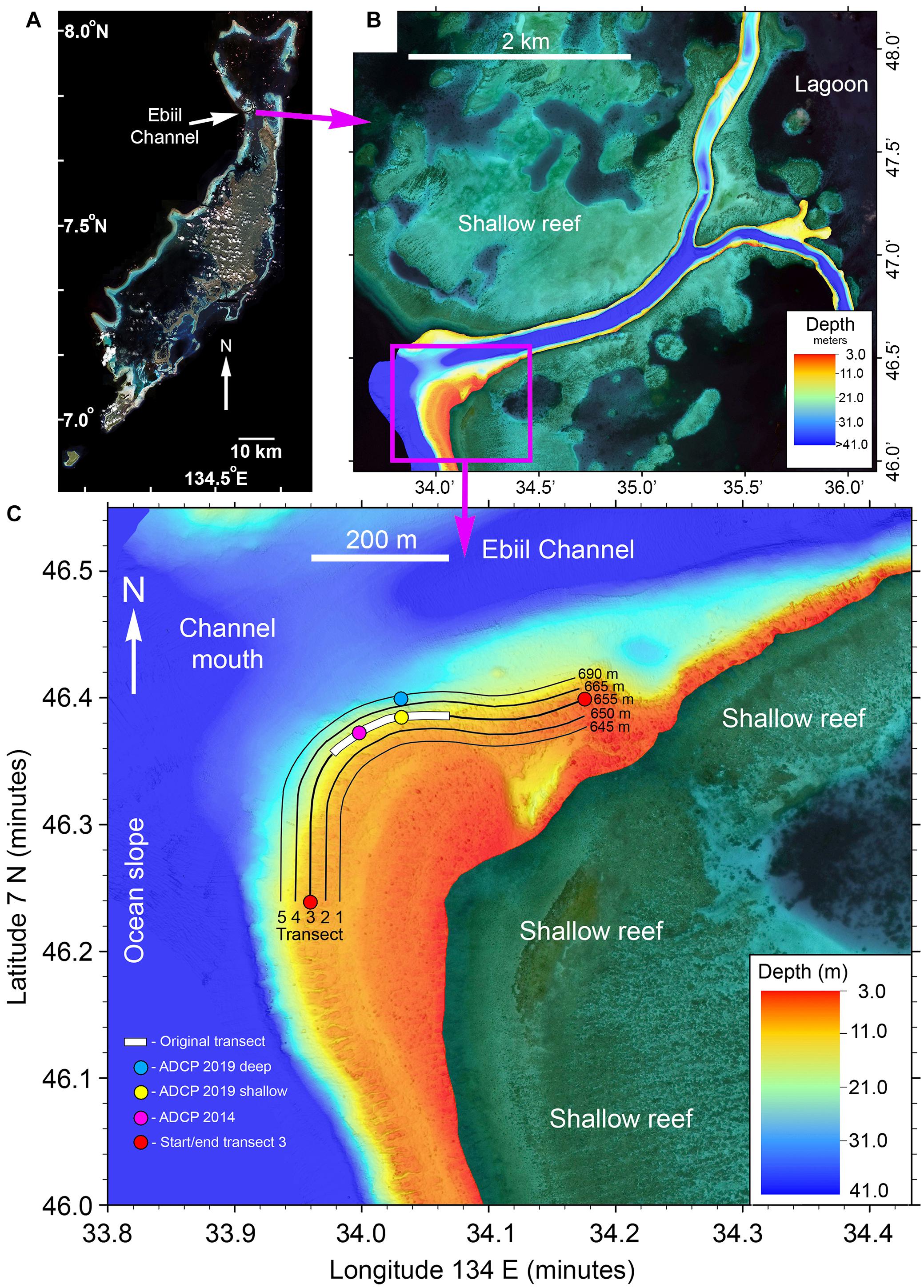
Figure 1. (A) Satellite image of the main Palau reef tract with the location of Ebiil Channel indicated. (B) Multibeam sonar map of Ebiil Channel showing depths from ocean to lagoon. The detailed area shown below is indicated by the purple box. (C) Multibeam map detail of the aggregation area at the southern side of the Ebiil Channel mouth. The five numbered survey transects are indicated with their lengths. The ends of the central transect (3) are indicated by red circles. The extent of the 200 m long original transect, variously used by earlier researchers, along transect 3, is shown by the white bar. The locations of acoustic doppler current profilers (ADCP) are shown.

The entire Ebiil channel was surveyed in March 2020 from ocean to lagoon using a WASSP multibeam sonar (Electronic Navigation Ltd., New Zealand) providing a detailed image of the aggregation site and adjacent areas. Data were plotted using Quick Terrain Modeler (Applied Imagery, Chevy Chase, MD, United States) to produce final maps (Figure 1B).

Survey Design: Temporal

Field surveys were conducted relative to lunar phase during spawning seasons in 2009 (6 lunar months–34 days), 2014 (3 months–18 days), and 2019 (2 months–8 days); 60 days in total. The 10-year span and 5-year survey intervals were considered appropriate to encompass the range of ages to first sexual maturity of the three species (P. areolatus; 2 years; E. polyphekadion; 4–6 years: E. fuscoguttatus; 9 years) (Pears et al., 2006; Rhodes and Tupper, 2008; Rhodes et al., 2011, 2013; Ohta et al., 2017). The 2009 surveys were done from April to September, covering the spawning season for the three species based on previous studies, and to inform planning for later work (Supplementary Table 1). Subsequent surveys focused on the months (June–August 2014 and late June–late July 2019) when peak numbers for the species were expected to occur in the week before new moon (BNM).

UVC surveys were conducted each lunar month over 4–7 days starting between 4 and 6 days BNM, weather permitting, and if fish were still present also on the day of the new moon (NM). Survey periods were planned to precede and include the day of peak abundance for each species, then continue until aggregations dispersed. Five planned survey days had poor weather preventing access to the site (although two of these days had supplementary photo records), with a total of 60 days successfully surveyed.

As our survey design was focused on counting all fish visible in the aggregation to quantify changes in total abundance (i.e., fish numbers) over time, daily counts were used as replicates to analyze the significance of these changes. We focused our analysis on the three main aggregation months of June, July, and August, however, in 2019 the new moon period fell between typical calendar months, so we only sampled two periods (late June and late July). To avoid comparing days when we counted few fish due to the aggregation dispersing, and to keep consistent between months and years, for analysis we used only the 3 days of highest counts each month. To analyze variations in fish abundance over time we used generalized linear mixed effects models (GLMMs) as they are well-suited to ecological count data, including unbalanced repeated measures designs (Pinheiro and Bates, 2000; Bolker et al., 2009). As our data were fish count data, we fitted GLMMs using a Poisson distribution (log-link), and a Laplace approximation (Bolker et al., 2009) with the lme4 package (Bates et al., 2015) in the R language and environment (R Development Core Team, 2020). As these data were not over-dispersed, we present pairwise tests between years using z-tests from the emmeans package in R (Lenth, 2020).

Survey Design: Spatial

Each field day, a three-diver team surveyed the five transects (Figure 1C) over two dives covering the entire aggregation area (with the center transect 3 surveyed twice). Each transect survey swim took between 25 and 35 min, with direction taking advantage of prevailing currents (most often moving from ocean into lagoon). Divers entered the water at fixed surface buoys marking the start and end of the center transects (Figure 1C). On the first dive of the day, one surveyor swam along the central marked transect while the other two surveyors stayed in visual contact (about 20 m apart from each other in good visibility) to cover the two deeper transects (4 and 5) while adjusting their swimming speed to stay aligned to one another. The numbers of all three grouper species observed by each diver within approximately 10 m to either side of their transect (roughly half the distance between divers) were recorded each minute of the survey. After completion of the dive and at least a 1-h surface safety interval, the three divers covered the shallower transects (1 and 2) with the central one (3) repeated, usually by the same individual as during the first survey dive. Data from the first and second surveys of transect 3 each day (32 days and three species) were found not to be statistically different (Pearson’s ‘r’ = 0.961; df = 94; p < 0.0001) and for consistency only the first survey of the day on this transect was used in subsequent data analysis. The daily sum of counts from these five transects was used as our measure of total abundance.

The spatial extent of the area occupied by each species was mapped during 2003-2008 pilot studies, i.e., prior to the first, 2009, survey. Five UVC transects (Figure 1C) covering the site were identified and georeferenced using position-logging Global Positioning System (GPS) receivers. The central transect (number 3) was marked at intervals on the reef by vertical metal rods (first installed, in part, in 1996) and the parallel shallower (numbers 1 and 2) and deeper (numbers 4 and 5) geolocated transects were physically marked at the start and end of transects and had distinctive topographic features for guidance of surveyors. The central transect 3 is an extension of the shorter transect (Figure 1C) used by Johannes et al. (1999) and later modified by Golbuu and Friedlander (2011) and the Palau Conservation Society [PCS] (2001, 2010). Transect 3 endpoint coordinates are: (west end) 7° 46.239′N; 134° 33.960′E; (east end) 7° 46.399′N; 134° 34.176′E.

The GPS density UVC method uses a position logging GPS receiver in a waterproof floating housing towed by a line attached to the diver below, recording the divers’ position on the transects (Colin et al., 2003, 2005) and providing quantitative position/time information along each transect. In 2009, all divers towed GPS receivers, logging positions every 30 s, and had waterproof watches synchronized with the time displayed by the GPS receiver. Fish were counted and data recorded each minute from the start of the survey. The area surveyed each minute was calculated from the distance traveled (recorded in the GPS position log) times the swath width (typically 20 m). Fish density was determined by dividing the number of fish counted by the area (m²) for each georeferenced minute-by-minute position. These density values were plotted on a latitude/longitude grid producing bubble plots to visualize and compare the spatial distribution of fishes.

To simplify surveys in 2014/2019, GPS receivers were not carried by all divers but start/stop times of the transect surveys were recorded. As the length and georeferenced position of the transects were known and could be replicated in subsequent years, we calculated density values (for each minute of the survey) from the 2019 data by dividing the transect length (Figure 1C) by the number of minutes required to cover the transect length on each dive. Density was expressed as fish per 100 m² and plotted over the length of each transect to show spatial changes in fish density along the horizontal length of the aggregation and depth gradients of the five transects (Figure 1C).

As fish density is often used as a proxy for total abundance when an entire aggregation cannot be surveyed, we compared the relationships between fish density (fish per 100 m²) and abundance (number of fish) using linear regression. Mean density values were calculated from the 20 highest densities of each species recorded during minute counts for each survey day. Minute counts along transects covered on average 20.4 m of distance and an area of ∼400 m² (transect swath 20 m wide). We included data from all surveys in June/July/August 2009 and June/July 2019 and plotted relationships of mean fish density versus abundance (from daily total abundance counts). To compare the slopes of the relationship between the three grouper species, we ran pairwise t-tests on the linear models using the emmeans package in R (Lenth, 2020).

Imaging and Body Size Data

Still Photography and Video

In addition to fish counts, time-lapse cameras were installed at key locations within the aggregation site in 2014 and 2019 to supplement data collection. Our interest was to examine fish behavior when divers were not present and to try to pinpoint the likely timing of spawning as well as of fish entry or exit from the study site in selected locations. Such information could be important because fish behavior on aggregations can be highly dynamic and divers were only present for less than 2% of available daylight hours on the site. GoPro^® cameras fitted with custom battery packs allowed multiple days of operation. Images were taken once per minute (2014) and 6 times per minute (2019). Some camera systems in 2019 recorded video for 15 min intervals (with a 1 min break between) over a 13-h period to try and capture night spawning. These were fitted with red (620–630 nm) LED lights; assumed to be outside of the visible detection spectrum of many reef fish (Fitzpatrick et al., 2013). For 2014 data, the numbers of each species in one still image were counted once every 5 min (adjacent images were checked if any details were in question), and numbers plotted over time. We partitioned counts as “benthic” and “midwater”, the latter if fish were ∼2 m or higher above the benthos. Any groupings, activity high in the water column, different color forms and gravid females were noted.

Body Size Measurement

The sizes of fishes at the aggregation were measured during surveys in August 2014 and June/July 2019 using a diver-operated stereo-video system (stereo-DOV; Goetze et al., 2019), first available to us in 2014, to determine any changes in body sizes over time which could indicate new recruits and to establish the size range of fish aggregating. This system consists of two video cameras in underwater housings mounted separately on a base bar, their fields of view converging at a fixed angle (∼6-degree inwards convergence). The diver using the stereo-DOV followed behind the UVC dive team, and roved across transects aiming the stereo-DOV system at any groupers encountered recording them when in clear view and perpendicular to the camera. This system enables determination of accurate fish total length measurements during post-processing of video footage (Harvey et al., 2010). The stereo-video system was first calibrated using the CAL software by SeaGIS and then analyzed using EventMeasure–Stereo software¹.

Physical Conditions

Currents at the site were measured by Acoustic Doppler Current Profilers (ADCP) during aggregation seasons in 2009 (Nortek ADCP 15 m) and 2019 (Teledyne SV 50 ADCP at 15 and 30 m depth). These instruments also record water depth (tides) during their deployments. In 2014 a single Onset Computer Inc. pressure logger was deployed to measure tidal patterns. Water temperatures were monitored with Onset U-22 temperature loggers (TL) over multiple months although not continuously over the entire period of our work. Deployments were typically for 6–12 months at depths of 15, 21, and 30 m with sampling at 30-min intervals. During the 2019 ADCP deployment RBR Solo TL (1 min sample interval) were installed on the ADCPs.

Results

Temporal Patterns; Annual and Monthly Peak Abundances

The highest number of fish recorded on a single day from each year, considered to be the annual peak abundance, showed a clear increasing trend for the fastest growing species, P. areolatus, with a near fourfold increase of 459–1,809 fish between 2009 and 2019 (Figure 2A). A more modest increase was recorded for E. polyphekadion and no change for E. fuscoguttatus. In addition, these three species also showed different patterns of abundance between months (Figures 2–5). Below we summarize these temporal patterns in abundance for each species separately.

FIGURE 2

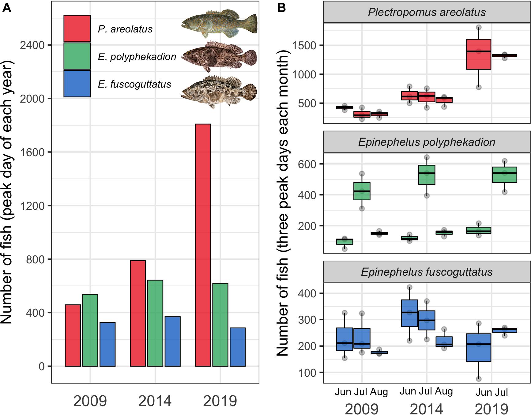
Figure 2. (A) Annual peak number (abundance) of fish recorded on daily surveys conducted during 2009, 2014 and 2019 for P. areolatus (red), E. polyphekadion (green), and E. fuscoguttatus (blue) at the Ebiil channel aggregation site. (B) Fish abundance from the three highest daily counts during the peak months (June, July, and August) of 2009, 2014, and 2019. Fish illustrations by Les Hata SPC.

FIGURE 3

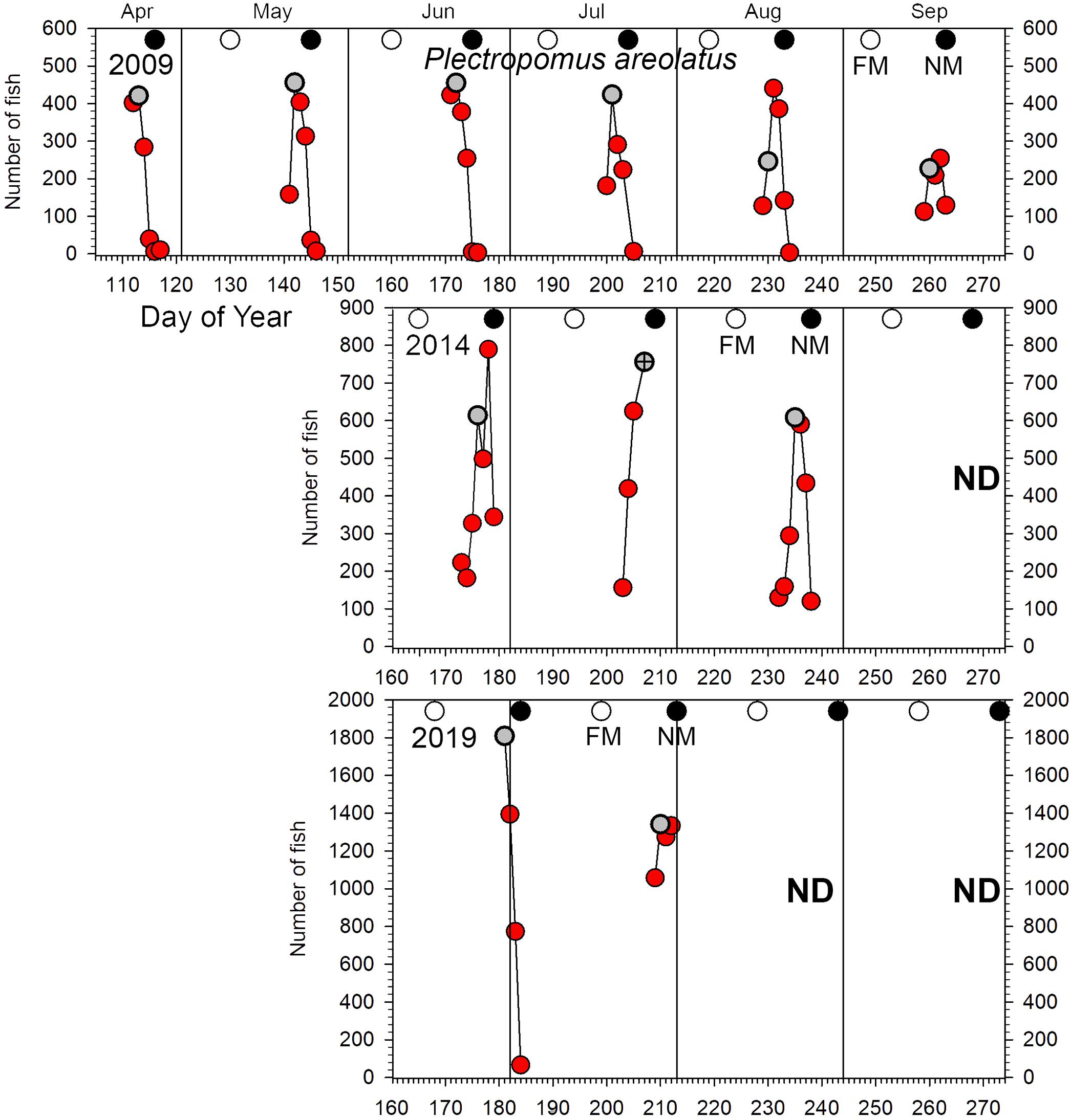
Figure 3. Number of P. areolatus counted in UVC surveys across the Ebiil site in 2009, 2014, and 2019 for the major aggregation period by day of the year and relative to full and new moon phases. The gray circles indicate day 3 before new moon (3 BNM), except for July 2014 when poor weather cut short surveys; for this month the symbol has a cross in its center and indicates 2 days BNM. Note differences in y-axes across years. ND, no data.

FIGURE 4

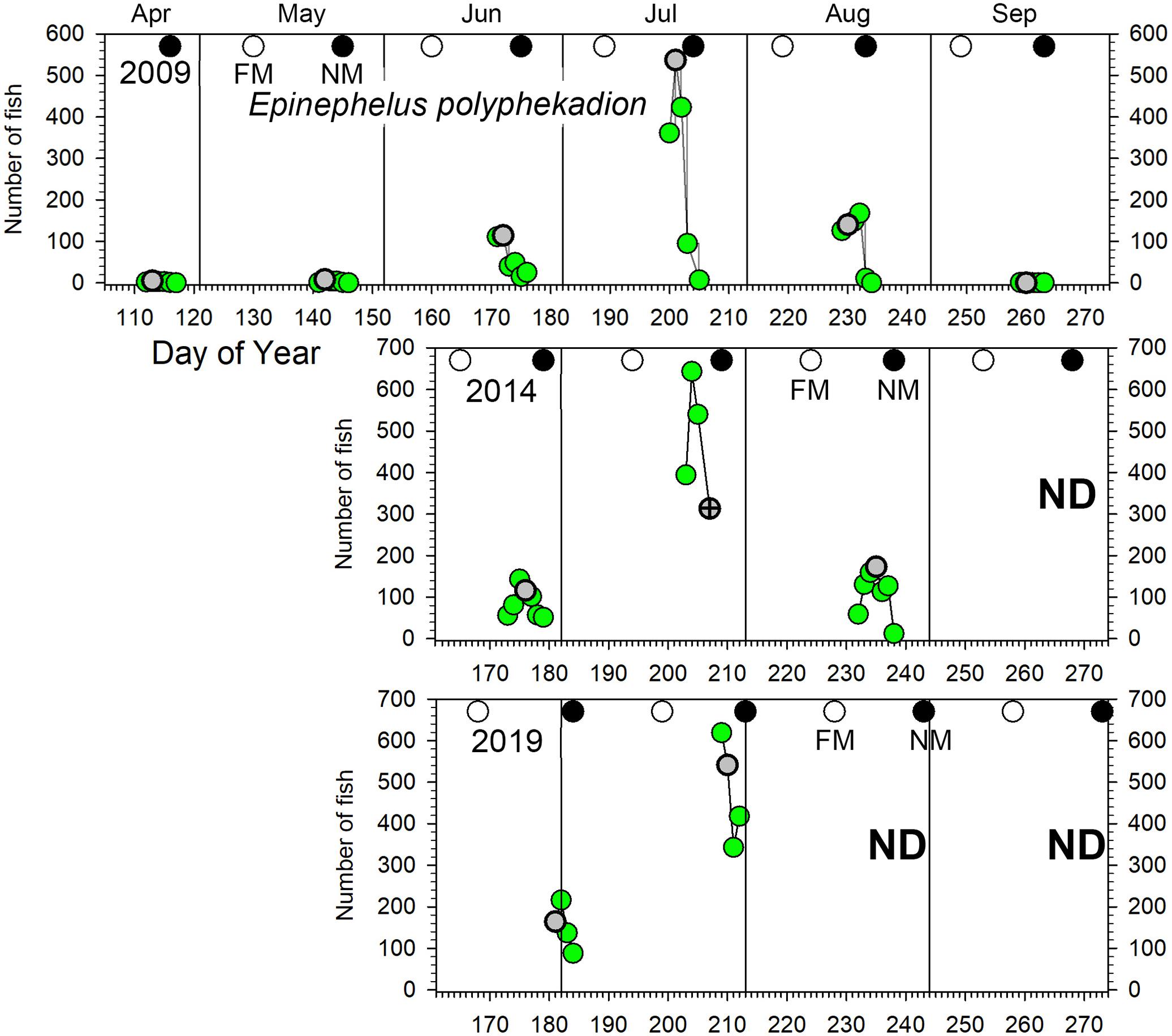
Figure 4. Number of E. polyphekadion counted in UVC surveys across the Ebiil site in 2009, 2014, and 2019 for the major aggregation period by day of the year and relative to full and new moon phases. The gray circles indicate day 3 before new moon (3 BNM), except for July 2014 when poor weather cut short surveys; for this month the symbol has a cross in its center and indicates 2 days BNM. Note differences in y-axes across years. ND, no data.

FIGURE 5

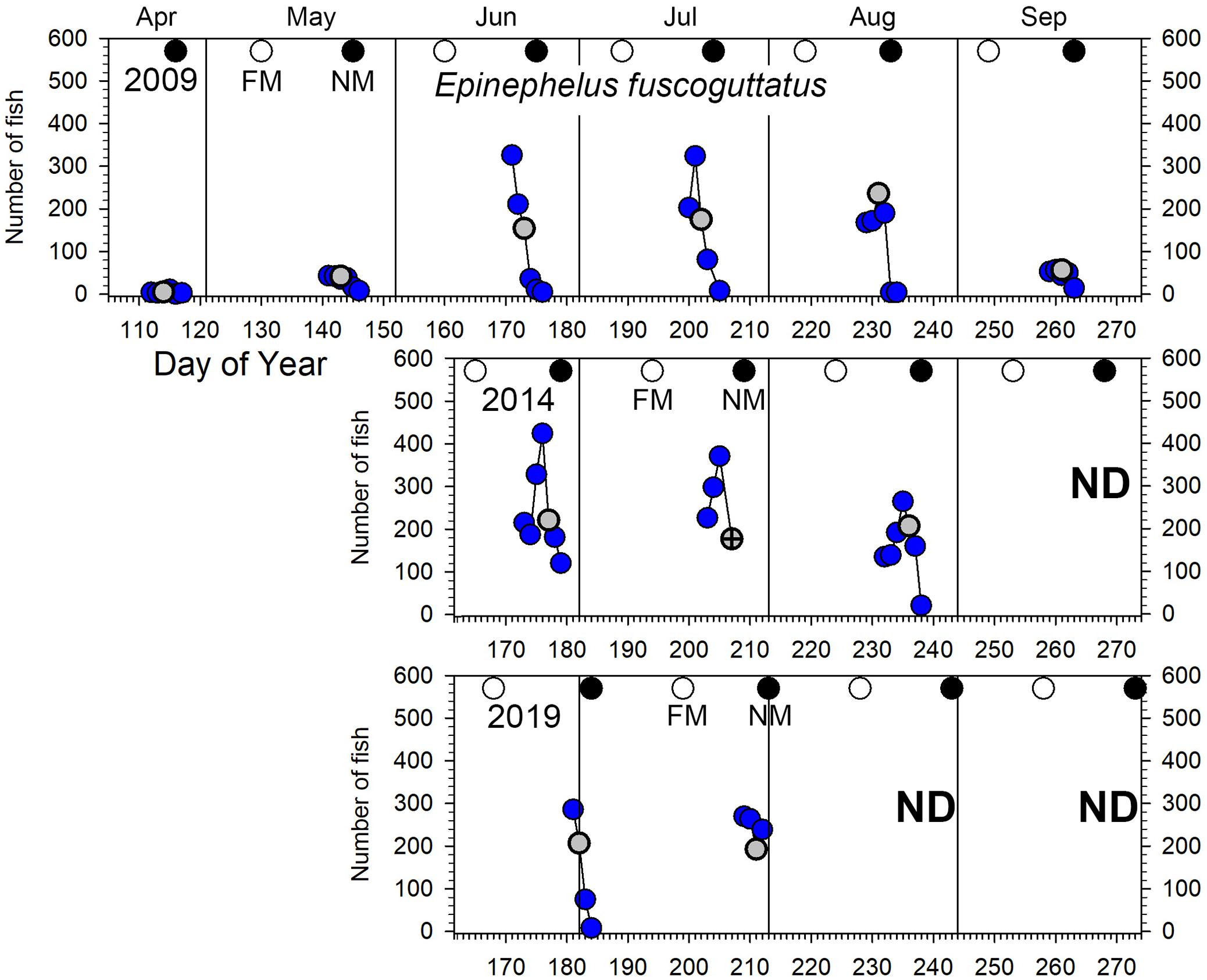
Figure 5. Number of E. fuscoguttatus counted in UVC surveys across the Ebiil site in 2009, 2014, and 2019 for the major aggregation period by day of the year and relative to full and new moon phases. The gray circles indicate day 3 before new moon (3 BNM), except for July 2014 when poor weather precluded surveys for which the survey 2 days BNM is displayed with a cross in the gray circle. ND, no data.

While we intended to visit the site daily starting at least 5 days before and up to the new moon, 5 planned survey days (July 22, 2009; July 24 and 26, 2014; June 29 and August 01, 2019) were missed due to bad weather which precluded access to the site. Counts by species for each of the 60 survey days are included in Supplementary Table 2.

The lunar timing relative to the peak daily numbers of aggregating fish (≥100) varied somewhat among species (Figure 6). P. areolatus numbers peaked most often 3 days BNM, but peaks could also occur on 1–2 days BNM (Figures 3, 6). E. polyphekadion had the broadest range, 1–5 days BNM (Figures 4, 6), while E. fuscoguttatus peaked between 2 and 4 days BNM (Figures 5, 6).

FIGURE 6

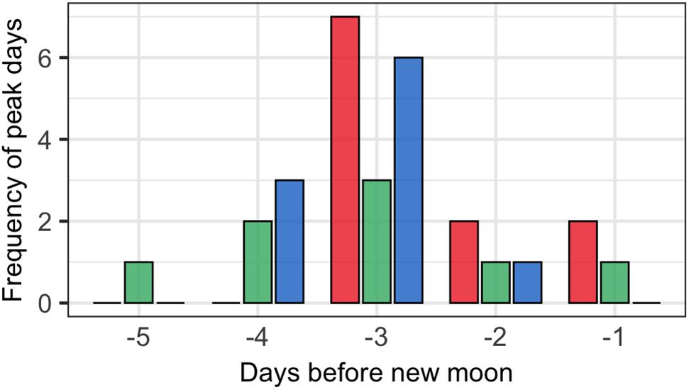
Figure 6. Lunar day BNM with peak monthly abundance of fish numbers for groupers (P. areolatus -red bars, E. polyphekadion -green bars, and E. fuscoguttatus -blue bars) for all surveyed months (2009, 2014, and 2019).

Plectropomus areolatus: elevated numbers (≥100 fish) occurred on the site for multiple months each year (Figure 3). Annual peak daily numbers roughly doubled between 2009 and 2014 (459–789 fish) and again from 2014 to 2019 (789–1,809 fish) (Figures 2A, 3). GLMM analysis of replicate daily counts (Figure 2B) showed significant (p < 0.0001) increases between years (Supplementary Table 3). Monthly peak abundance exceeding 400 fish remained stable from April to August 2009, but declined in September to about 50% (200 fish) of earlier peaks (Figure 3). In 2014, monthly peak abundances were higher than in 2009, being greatest in June (near 800 fish), then dropping to 600 by August. In 2019, monthly peak abundances were greater than in 2014, with 1,800 fish in June and decreasing to near 1,300 in July. In 2019 several groups of 3–50 small (200–300 mm) dark-colored P. areolatus were seen roving across and within the site, something not observed in 2009 or 2014. These were included in daily counts (Figure 3).

Epinephelus polyphekadion: we recorded these fish aggregating with daily numbers ≥100 fish occurring for 2–3 months each year with only 1 month showing markedly elevated values (Figure 4). In 2009 a major peak in numbers occurred in July (over 500 fish), 3–5 times larger than adjacent months (i.e., June and August). In 2014 a similar pattern occurred for changes month to month and overall numbers. In 2019, the survey in late July was the peak month, and based on the pattern from previous years we did not expect higher numbers the following month in late August so surveys were not conducted. Across all surveys, peak daily numbers were stable at 500–600 fish, but with several indications of an increase by 2019. First, daily counts over all months showed a significant increase between 2009 and 2019 (p < 0.01; Supplementary Table 3). Second, fish density on the deepest transect (5) reached 17 fish per 100 m² in 2019 compared to 8 fish per 100 m² in 2009 (Figure 7 and see section “Spatial Patterns of Density and Abundance”). Brief diving observations of the channel bottom deeper than the study area in 2019 also indicated the presence of many more fish than observed in 2009 and 2014 during similar forays. Finally, a random survey swim deeper than transect 5 on July 29, 2019 (1 day after peak numbers were surveyed) resulted in a count of 76 fish. These qualitative observations also indicated many more E. polyphekadion beyond the deeper edge of this transect in 2019 compared to previous years.

FIGURE 7

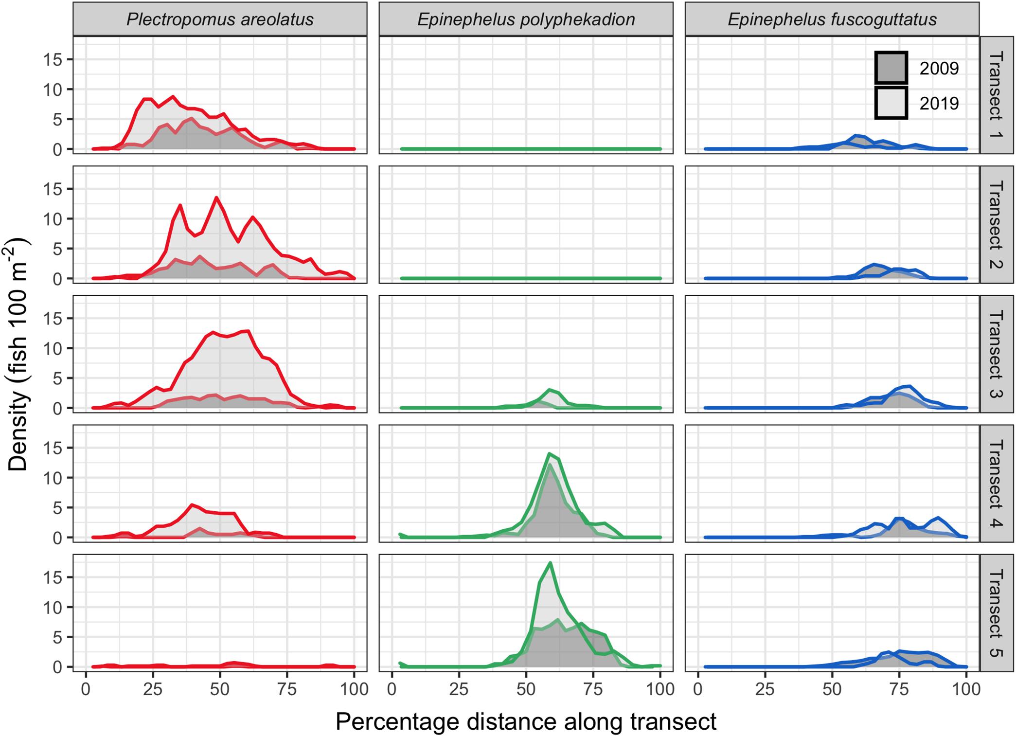
Figure 7. Fish density across the 5 survey transects by species for 2009 and 2019 with only days of annual peak abundances shown. Each row is a separate transect with transect 1 being the shallowest (8–12 m) and transect 5 the deepest (23–27 m). Densities for each species are shown relative to their location along each transect as a percentage of the distance from the start (0) to the end (100). Transect length is about 650 m and swath width of 20 m; direction is from the outer reef toward the lagoon (Figure 1).

Epinephelus fuscoguttatus: elevated numbers (≥100 fish on the site) were observed from June to August (Figure 5) with no indication of change in abundance over the decade (all pairwise tests p > 0.05, Supplementary Table 3 and Figure 2). Highest daily numbers varied from about 300–450 individuals across the three survey periods. Considering individual years, values were similar for the first two aggregation months (June/July) and lower in the following month (August) for 2009 and 2014 (Figures 2B, 5). The 6-month sampling period in 2009 (Figure 5) recorded low numbers during April and May (fewer than 50 individuals), followed by three peak months, then lower numbers in September (near 50 maximum individuals).

Spatial Patterns of Density and Abundance

We surveyed the entire aggregation area of P. areolatus and E. fuscoguttatus; however, we were not able to cover the full extent of the distribution of E. polyphekadion as its deepest occurrences spread outside the diving depth limitations. The GPS and time-referenced counts along transects quantified the spatial distribution of fishes across the 650 by 100 m study site. Plots of density (fish per unit area) data from the five transects on their respective days of annual peak abundance for 2009 and 2019 indicate that each species has a distinct area within the site where it gathers. There is some overlap between P. areolatus and E. polyphekadion (transect 4) and between the two Epinephelus species (transects 3–5) (Figures 1, 7, 8). P. areolatus predominantly occurs on shallower (transects 1–3) and E. polyphekadion on deeper transects (transects 4–5). E. fuscoguttatus occurs toward the lagoon end of the site and covers a wider depth range than other species. P. areolatus and E. polyphekadion have limited areas within the aggregation where their densities were clearly highest; such concentration was not so evident in E. fuscoguttatus (Figure 7).

FIGURE 8

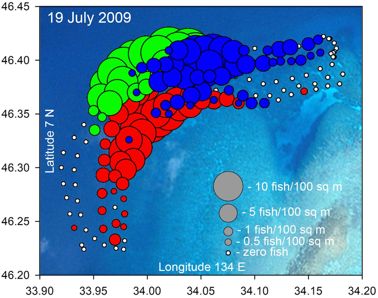
Figure 8. Example bubble plot for the Ebiil aggregation site from July 19, 2009 indicating density (fish/100 m²) counted along five transects for P. areolatus (red), E. polyphekadion (green), and E. fuscoguttatus (blue). This was a day of high abundance with (respectively) 324, 537, and 424 individuals counted. Some bubbles for E. polyphekadion and P. areolatus are masked by overlying blue bubbles of E. fuscoguttatus. Small white dots indicated no fish at that location. Variations in transects from design (Figure 1) were due to surveyors or their towed GPS drifting slightly off track, as evidenced by GPS position logging.

To visually represent spatial relationships among the three species on the study site a bubble plot was constructed (Figure 8). This plot shows the three grouper species overlapping in certain areas but also showing overall differences in distribution which were consistent among years.

Plectropomus areolatus: comparisons of fish density between 2009 and 2019 (Figure 7) showed that the fourfold increase in abundance (Figure 2) did not necessarily translate to increased densities in areas where fish were originally observed in their greatest densities. For example, in 2009, densities were highest on the shallowest transect (transect 1) reaching 5 fish per 100 m², however, densities on that same transect in 2019 only reached 9 fish per 100 m² and the highest counts were, instead, on the deeper transects (transects 2–3), reaching densities of 13 fish per 100 m².

Relationships between abundance and density for 2009 and 2019 are linear, up to almost 500 fish and 5 fish per 100 m² (Figure 9). Beyond those levels the relationship becomes curvilinear with increases in abundance associated with progressively smaller increases in density. Assuming the relationship between fish density and total abundance remained linear (y = 0.009^∗x−0.002), a doubling of density from 5 to 10 fish per 100 m² would predict a total abundance of 1,100 fish, however, our data points from greater abundance counts reveal total abundance would more than triple (from 550 to 1,750 fish). Our curvilinear relationship shows a tendency toward an asymptote suggesting that there may be maximum densities for aggregations of this species and that at some level increases in fish numbers would be reflected only in increased aggregation area, i.e., by fish spreading out, rather than higher densities. This potential may account for the spatial expansion across transects between 2009 and 2019 (Figure 7).

FIGURE 9

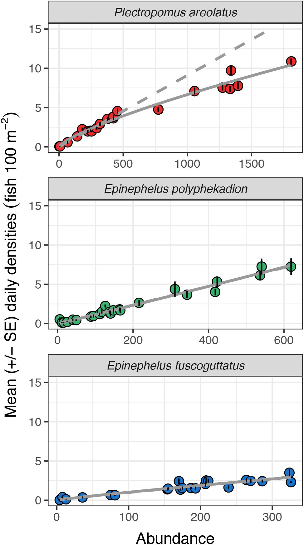
Figure 9. Mean daily densities (fish per 100 m²) and standard errors against total study site UVC abundance values for P. areolatus, E. polyphekadion, and E. fuscoguttatus on all survey days in June, July, August 2009 and June, July 2019. Each point represents the mean of the 20 highest densities recorded during minute counts for each day.

Epinephelus polyphekadion: the relationships between density and abundance for 2009 and 2019 are linear (y = 0.012^∗x−0.023;Figure 9). The slope of the linear regression was significantly (p < 0.01) steeper than for the other two species (Supplementary Table 4) with densities higher at comparable abundance levels. As for P. areolatus, maximum mean density exceeded 7 fish per 100 m². Unlike P. areolatus, there was no suggestion of fish spreading out within the survey area as density increased (see transect 5, Figure 7), although qualitatively more fish were noted deeper in 2019 outside of the survey area (see above), so some spread appears to have occurred outside our survey area. Examination of abundance at higher densities is necessary to determine whether the relationship starts to become non-linear; elsewhere aggregations of this species may reach many thousands of fish and much higher densities (see Supplementary Figure 1).

Epinephelus fuscoguttatus: the relationship between density and abundance for 2009 and 2019 appears linear (y = 0.009^∗x + 0.105). With maximum values of about 4 fish per 100 m², its density is less than half that of the other two species. As with E. polyphekadion, examination of abundance at higher densities is needed to determine their relationship since aggregations of this species elsewhere can exceed 1,000 fish (Seychelles, Robinson et al., 2008; Pohnpei, Rhodes et al., 2014).

Imaging and Body Size Data

Still Photography and Video

Autonomous photography at the study area during aggregation periods produced over 50,000 images in 2014 (37 days) and 2019 (9 days). These complemented UVC data and divers’ notes, providing a visual record of activities in selected areas during daylight hours (approx. 5.30 am–6.30 pm) including in the absence of divers. We present time-lapse data from 6–10 days of continuous filming from three camera stations in June, July, and August 2014 (Figure 10). Counts reflected the number of fish visible to the camera and do not indicate absolute fish abundance on the site. Greater proportions of E. fuscoguttatus were observed in the midwater during early mornings and early afternoons, which also coincided either side of our dive survey times (Figure 10B). This pattern of lower fish numbers, especially in midwater, was most pronounced at the times of dive surveys indicating that diver presence may be affecting the normal activity and counts of this species. Generally, we observed that this larger species is more wary of divers compared to the other two species and quickly retreats to shelter within the reef structure when approached; this was apparent in sequential still shots as divers approached and then passed stationary cameras, with fish emerging over the following 20 min or so.

FIGURE 10

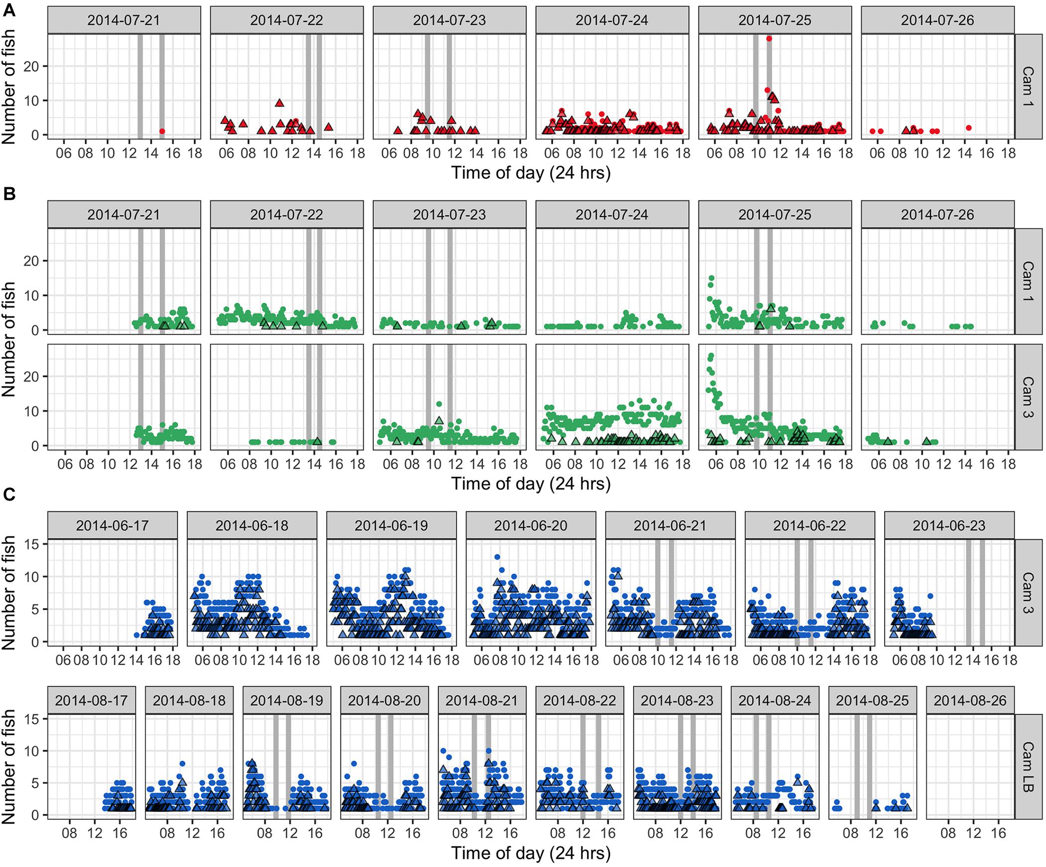
Figure 10. Number of fish counted in images taken with time-lapse mode camera operation in 2014 at selected locations within the Ebiil study site. Circles represent benthic and midwater counts combined, while triangles indicate midwater counts only. Vertical gray bars represent dive survey times (two dives per day). (A) P. areolatus July 21 to 26, 2014; peak abundance for that month was July 25 (although no dive was possible on 24th); (B) E. polyphekadion. Two cameras (Cam 1 and 3) located in different areas of the survey site recorded from July 21–26th, peak abundance was on July 22. (C) E. fuscoguttatus prior to and during the June survey period, but camera battery ran out at 10 am on June 23rd, a day before the peak abundance. In August 2014, peak abundance was on August 22 with fish leaving the site on the 25th.

In addition to quantitative data for selected cameras, a qualitative summary of observations over all camera deployments is given for each species. The value of this autonomous documentation was further highlighted when poor weather precluded diver presence on 5 days between 2009 and 2019 (Supplementary Table 2), of which 2 days had time-lapse images. Images on July 24, 2014 revealed similarly high relative fish numbers to the following day when surveys could be done, whereas images from the missed survey on July 26, 2014, reveal that fish had dispersed from the aggregation (Figures 10, 11).

FIGURE 11

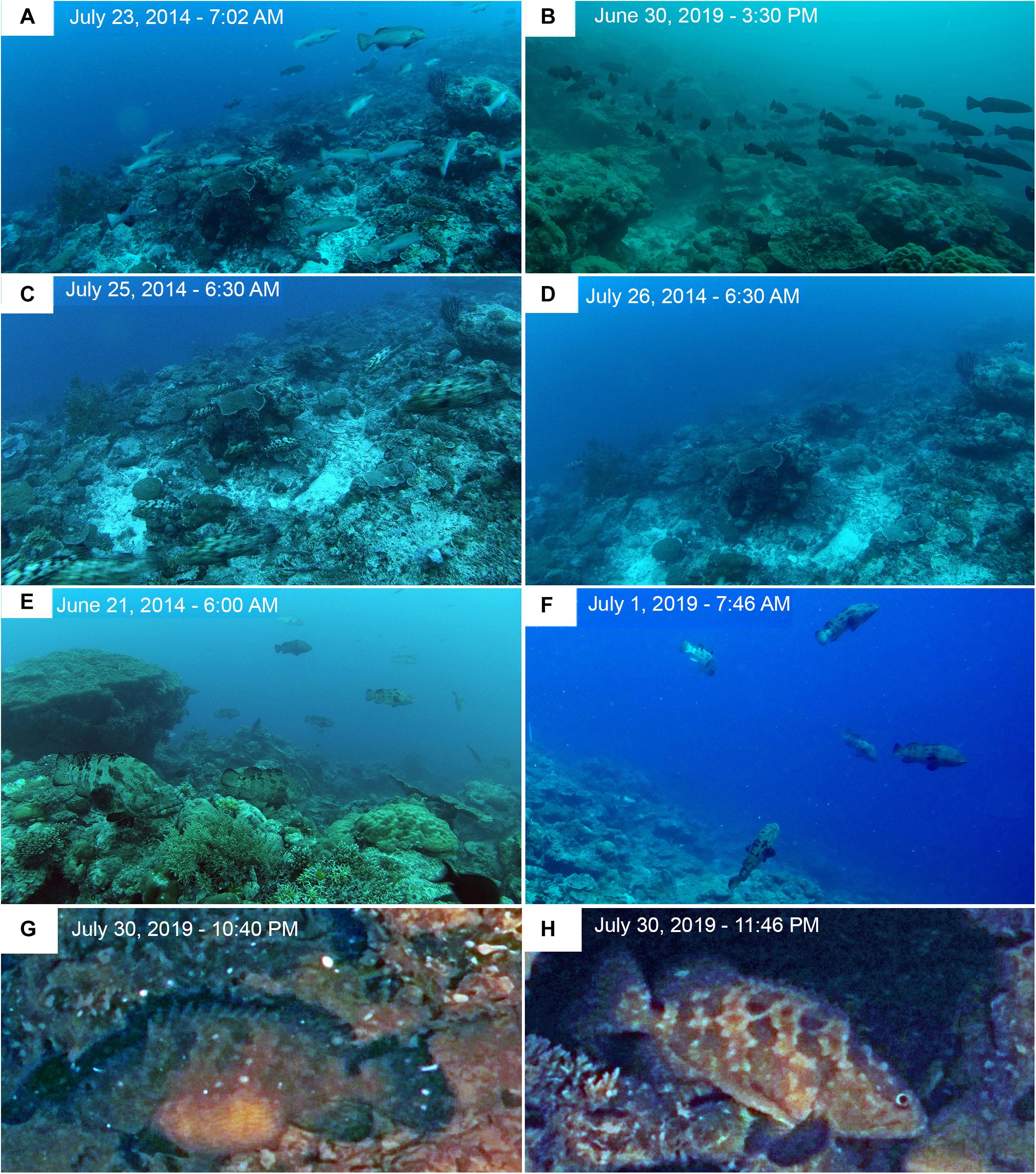
Figure 11. Time-lapse images at Ebiil Channel in 2014 and 2019. (A) P. areolatus – Adults moving across site a day or two before peak numbers. (B) P. areolatus – School of small dark fish moving across site on day of peak count for the species. (C) E. polyphekadion – At first light, fish streaming out of the site; peak day had been on July 22, 3 days earlier. (D) Same location day on following morning. (E) E. fuscoguttatus – Fish up in water column where they spend a large proportion of the day, chasing, and changing colors. Some individuals remain stationed high above the substrate for extended periods as new moon approached. Numbers built to peak abundance on June 24 but fish were active, including above substrate for several days before hand, such as indicated in the image. (F) E. fuscoguttatus – Image taken on day of peak abundance for this species in June 2019. Multiple fish moved quickly between substrate and water column to form small interactive groupings. Note white survey stake in mid-left background at edge of image. (G) Night image (color corrected from red light) of a gravid female E. polyphekadion with extremely swollen abdomen (for more information on G,H; see Supplementary Material). (H) Image of a female E. polyphekadion, presumably the same fish, in the same location, 1 h later with a deflated abdomen.

Plectropomus areolatus: larger adults generally stayed within, and appeared to defend, circumscribed areas for extended periods as determined by repeated sightings of several individuals, likely males, with distinctive individual markings in images, and frequent chasing. Smaller females (sometimes clearly gravid) appear to be more mobile, and remained closer to the substrate. Divers noticed groups (3–50 fish) of small dark-colored fish moving around the site only in 2019 which were captured on time-lapse camera (Figure 11B) and were measured by stereo-video (Figure 12). Activity level was generally lower in the latter part of each day, and increased overall until the last day of the aggregation. The following morning fish had dispersed (Figures 10, 11).

FIGURE 12

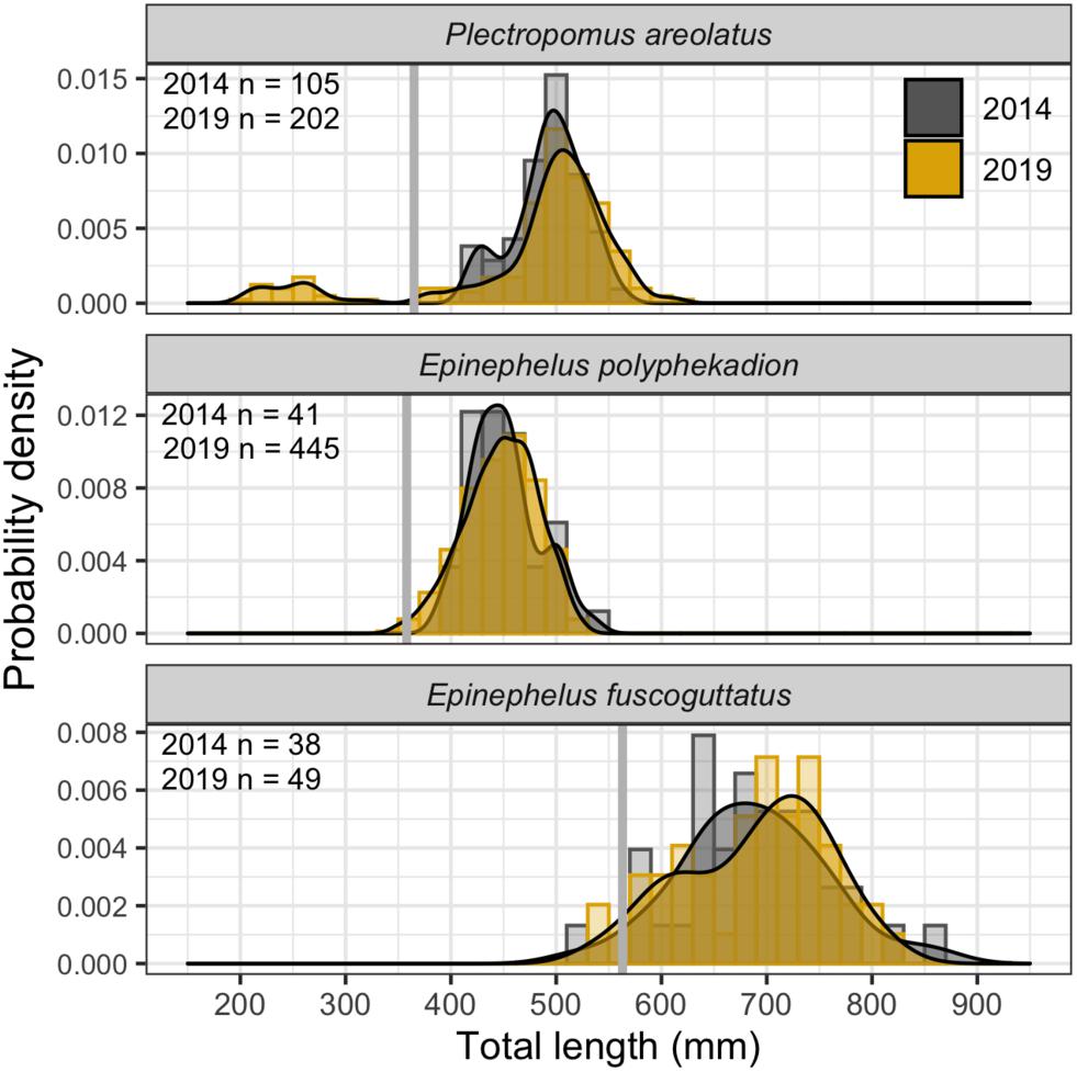
Figure 12. Size frequency distributions for 2014 and 2019 and sample sizes by species and year. Probability density curves are displayed over frequency histograms of total length (20 mm wide bins). 2014 data filled as gray and 2019 data as yellow. Mean estimates of size at maturity (L_50%) from Palau are shown as gray vertical bars.

Epinephelus polyphekadion: activity increased overall, as determined by fish counts in images, until the last day of the aggregation in July 2014, after which fish quickly left the site on the early morning of July 25 in large groups (Figures 10B, 11C). Similar prompt disappearance was noted in July and August 2009. Individuals stayed in the same general area for multiple days, as determined by recognizable distinctive individuals. For example, a distinctive yellow color morph was photographed multiple times on different occasions in one area and twice in open mouth-to-mouth combat with other males in the same area.

Epinephelus fuscoguttatus: fish were often actively chasing other groupers, as well as conspecifics, based on time-lapse images and diver records. Chasing and color changes through various mottled shades to an almost white phase with dark caudal peduncle and blotches still visible were regularly photographed for multiple days leading up to the peak day in 2014 (June 24), as well as in August 2014 when abundance and time-lapse counts were lower (Figures 10, 11). Fish were active up in the water column during most daylight hours, with less activity evident overall in the middle of the day and with divers present. Sequences of images from early mornings (6–9 am) over several days during the aggregation period show fish rising substantially above the benthos and some instances of pairs heading higher in the water close to the surface and descending soon after. But as time-lapse images were shot at 1 min or 10 s intervals, spawning could not be confirmed (please see Section “Physical Conditions”).

Body Size Measurement

Size frequency data (Figure 12) for P. areolatus (modal peak 502 mm, min/max TL 376/612 mm), E. polyphekadion (modal peak 451 mm, min/max TL 348/532 mm), and E. fuscoguttatus (modal peak 731 mm, min/max TL 522/861 mm) indicate that almost all fishes were above the mean size of female sexual maturation (L_50%). The groups of small dark-colored P. areolatus we only observed in 2019 (Figure 11B) formed a separate peak in length frequency (200–300 mm TL), suggesting that they are not yet sexually mature. Comparisons of length frequencies between 2014 and 2019 showed a high level of overlap.

Physical Conditions

Temperature

Shallow (above 15–20 m depth) outer reef waters in Palau range from about 27.5 to 30°C annually with the Ebiil patterns similar to those at other barrier reef areas in Palau (Colin, 2018). While we lack complete data for any calendar year at Ebiil, the known portions of the yearly pattern align with the daily mean temperatures at the West Channel, south of Ebiil, at 15 m depth (7°32.560′N; 134° 28.059′E).

June and July, peak months of aggregation, (Figure 13, dark pink highlight) have the highest annual water temperatures, consistently between 29 and 30°C. If the broader time when P. areolatus aggregates is considered (Figure 13, light/dark pink highlights), this includes the period with temperatures rising toward June’s highest annual temperatures and a gradual decrease in early fall. The upper 15 m of the water column over the aggregation site is unithermal, but temperatures at 30 m drop 2–4°C below those on the shallower reef for periods of hours (Supplementary Figure 2). These drops represent layers of cooler water being brought into the channel from offshore, or less commonly lagoon water exiting, and may be more common during El Niño periods in Palau (Colin, 2018).

FIGURE 13

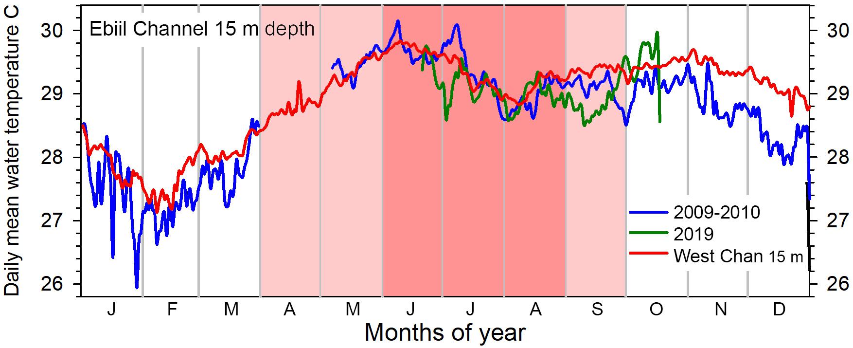
Figure 13. Annual patterns of daily mean water temperature at 15 m depth, Ebiil channel. Partial cycles of temperature were recorded in 2009–2010 and 2019 with gaps in the April to early May period. Similar data from 15 m in the West Channel, south of Ebiil, for the same years show the complete annual cycle and the close similarity of data between the two sites. The 6 months (April to September) with pink shading indicate those months with P. areolatus aggregation, while the darker pink 3 months (June to August) include time of aggregation of the other two species.

Current Speed/Direction and Spawning

In 2019 (as in 2009) current speed at the deep and shallow ADCPs never exceeded 0.73 m sec^–1 with 80% of measurements being below 0.32 m sec^–1. Any currents greater than 0.05 m sec^–1 at 17 and 30 m depths were directed, almost exclusively, along the axis of the channel on both outgoing and incoming flow. Strongest currents (over 0.6 m sec^–1) were oriented very narrowly at 245° for outgoing and 60° for incoming flow (Supplementary Figure 3). The volume of incoming (flood) and outgoing (ebb) flow over the 157 days of measurements by the deep ADCP in 2019 differed. Incoming currents occurred 62% of the time with an average speed of 0.3 m sec^–1 while outgoing currents occurred 38% of the time and averaged 0.24 m sec^–1, producing a net inflow volume roughly twice that of the outflow.

The new moon periods June 30 to July 3 and July 29 to August 01, 2019 are thought to represent times when spawning was occurring, evidenced by gravid females, fish stationing themselves high in the water showing color changes and aggressive interactions among individuals. The period of 30 June to 06 July had the strongest outgoing currents, reaching speeds over 0.4 m sec^–1 in the early morning, and over both these new moon periods the outgoing tidal flows were largely restricted to nighttime (Figure 14). Time-lapse cameras recorded E. fuscoguttatus individuals interacting high in the water column from dawn until about 8 am during July 1st and 2nd 2019 (Figure 11F) coinciding with the end of the outgoing tide and with generally slack current conditions. From the overnight recordings of gravid E. polyphekadion on July 30 (Figures 11G,H and Supplementary Material), we presumed a spawning time around 11 pm. This coincides with the end of the outgoing (flood) tide which had a relatively low flow rate, reaching a maximum speed of 0.15 m sec^–1 around 9 pm (Figure 14).

FIGURE 14

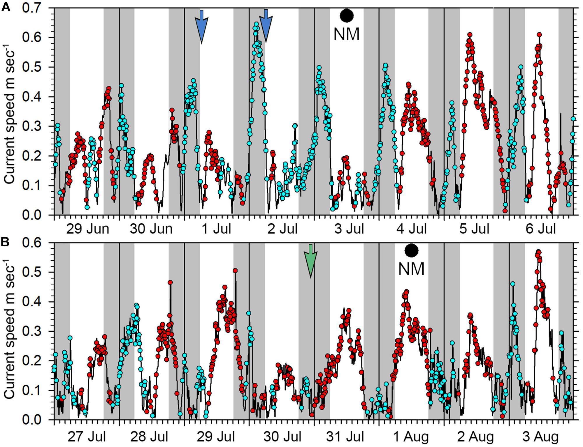
Figure 14. Current patterns at the Ebiil aggregation site from (A) 29 June to 06 July 2019, (B) 27 July to 03 August 2019. Blue dots represent outgoing current direction, red dots incoming. Night periods are indicated by gray shading, day by white background. The blue arrows on 01 and 02 July indicate time of heightened activity of E. fuscoguttatus while the green arrow on July 30 indicates likely spawning of E. polyphekadion on this date. New moons were July 03 and August 01.

Discussion

The decade-long UVC study of the protected Ebiil aggregation site in Palau showed significant increases in one grouper, P. areolatus, strong indications of increase in a second, E. polyphekadion, and apparent stability in the third, E. fuscoguttatus. The results highlight the importance and outcomes of effective protection, timeframes needed for recovery, and identify key considerations for designing UVC protocols that can reliably detect and quantify changes in fish numbers over time. We examine the temporal/spatial patterns of abundance indicated and their relationships to abiotic factors in Palau, and compare our results to those of other studies of the three species across their geographic ranges. We consider what these patterns reveal about aggregation dynamics and the relationship between abundance and density, the latter being a widely used indicator/proxy for fish abundance. Finally, we consider what our results, over a decade, indicate about the management at Ebiil to date and regarding planning for future protection.

Temporal and Spatial Patterns

The three co-occurring species at Ebiil Channel, within an overall pattern of shared aggregation season and location, differ somewhat in their distribution, aggregation duration, abundance, densities and timing of reproductive seasons, but also show patterns. They occupy distinctive, but overlapping, areas and are inter-specifically competitive (chasing) on borders where they overlap. In general, P. areolatus occupies shallower waters, down to about 20 m, as reported elsewhere (Sadovy de Mitcheson, 2011; Hamilton et al., 2012; Hughes et al., 2020), making it particularly susceptible to spearfishers. E. polyphekadion were observed from 15 m depth to the channel bottom at 35–40 m deep, with no deeper waters nearby. E. fuscoguttatus was most common in areas of large reef outcrops separated by sandy substrate in waters about 15 to 25–30 m. These depth ranges are consistent with those reported elsewhere with the exception of the Kehpara aggregation site in Pohnpei where all three species were found to at least 50 m on a steep outer reef wall (Rhodes et al., 2014), although P. areolatus was also found shallower than the other species.

Comparisons of density, abundance, SA formation relative to lunar cycles and duration of spawning season between this and other published studies revealed both similarities and differences. Results reveal geographic variability among and within species, providing opportunities for comparative analyses and highlighting the challenges of monitoring multi-species aggregations in a way that allows for reliable comparisons (Colin et al., 2013). Abundance at the Ebiil site built up for 7 or more days prior to the new moon to peak numbers and then dispersed quickly, presumably after spawning, around the day of the new moon. High numbers of P. areolatus sometimes occurred several days in succession in any 1 month, whereas a clear ‘peak’ of just one or 2 days was typically evident for the other two species (Figures 3–5 and Supplementary Table 2; Johannes et al., 1999).

Across geographic locations, peak aggregation abundance for the three species was associated with the days before/on either full or new moon, and, within a given location, all species followed the same lunar phase. However, duration and timing of aggregation annually can vary geographically. New moon aggregation/spawning, similar to Palau, was noted in the Solomon Islands (Hamilton et al., 2012; Hughes et al., 2020), Papua New Guinea (Hamilton and Matawai, 2006; Hamilton et al., 2011; Waldie et al., 2016), Kenya (Samoilys et al., 2014), Lakshadweep (India) (Karkarey et al., 2017), and the Seychelles (Robinson et al., 2008; Bijoux et al., 2013). Full moon spawning/aggregation was recorded in Pohnpei (Rhodes et al., 2014), Fiji (Sadovy de Mitcheson, 2011), and French Polynesia (Mourier et al., 2019; YSdeM, unpublished). Both new and full moon aggregations were noted for P. areolatus in Indonesia (Pet et al., 2005), and the Solomon Islands (Hamilton et al., 2012). It is not known what determines full versus new moon phase of spawning in different locations, but this difference may hold opportunities for understanding conditions determining reproductive success, or be linked to cues to aggregate.

Across geographic locations, species-specific differences occurred in duration and timing of the aggregation season. Duration of the spawning season in Palau varied by species, with P. areolatus aggregating over 5–6 months annually, E. polyphekadion for 1–2 months, and E. fuscoguttatus for 2–3 months (Johannes et al., 1999; this study). Geographically, the overall pattern of annual spawning season length among species was similar to Palau; generally longest for P. areolatus (at 4–6 months, occasionally more), shortest for E. polyphekadion (1 or 2 months) and intermediate for E. fuscoguttatus (2–4 months) (Rhodes and Sadovy, 2002; Rhodes and Tupper, 2008; Robinson et al., 2008; Rhodes et al., 2011, 2014; Hamilton et al., 2012; Bijoux et al., 2013; Samoilys et al., 2014; Waldie et al., 2016; Hughes et al., 2020). In terms of seasonality, aggregation for spawning from the Seychelles to the central Pacific cover all months of the year, although January to August are most commonly reported in the published literature (Passfield, 1996; Sluka, 2000; Rhodes and Sadovy, 2002; Pet et al., 2005; Robinson et al., 2008; Hamilton et al., 2011; Wilson et al., 2011; Bijoux et al., 2013; Rhodes et al., 2014; Samoilys et al., 2014; Mourier et al., 2016; Karkarey et al., 2017; Hughes et al., 2020).

Geographically, the abundances and densities of fish differed substantially by species and at least partially according to fishing pressure. Peak abundance of fishes over this study period at Ebiil ranged from hundreds (E. fuscoguttatus and E. polyphekadion) to almost two thousand fish (P. areolatus). Average fish density reached about 10 fish per 100 m² for P. areolatus, 7 for E. polyphekadion and about 3 for E. fuscoguttatus. Below we compare findings from other locations for each species separately. Based on data elsewhere for these species, on our observations, and considering historic reports in Palau, we expect that more years of recovery could bring numbers at Ebiil much higher than in 2019, especially in the case of E. polyphekadion.

For P. areolatus, reported aggregation sizes range from fewer than one hundred to three thousand fish, with densities from 1–2 up to 19 fish per 100 m² in core areas. The most fish reported in a documented aggregation was 3,046 fish (calculated from densities) with an average core density of 19 fish per 100 m² (Pohnpei; Rhodes et al., 2014). In Papua New Guinea, the maximum density at a protected site was 17 fish per 100 m² while two nearby fished sites had 10 and 14 fish per 100 m² with fish numbers at those sites ranging from 500 to over 1,000 (Hamilton and Matawai, 2006). Large numbers are inferred from a lightly fished aggregation in Lakshadweep (off India) (Karkarey et al., 2017), although the behavioral interpretations of this paper are refuted (Erisman et al., 2018). At the opposite extreme, an exploited Solomon Island site had a density of only 1.6 fish per 100 m² (Hughes et al., 2020). Other heavily exploited sites likewise had low abundances (less than 100 total fish), as in Indonesia (Pet et al., 2005).

Some reports have suggested that not all lunar-associated aggregations or groupings of this species are associated with spawning, highlighting the need to pay attention to other spawning-related behavior such as presence of multiple gravid females. Hamilton et al. (2012) proposed for the Solomon Islands, where both full and new moon gatherings were reported, that full moon gatherings were the start of fish numbers building toward spawning on the following new moon. In Pohnpei, both fishery-dependent and fishery-independent data indicate that only males are present during the first month of the annual aggregations (Rhodes and Tupper, 2008). Histological information suggests that ripe and spent female P. areolatus are only present for about 4 months although aggregations form for more months, i.e., January to May (Rhodes and Tupper, 2008; Rhodes et al., 2013). Moreover, the roving groups of small fish sometimes seen in larger aggregations (and in 2019 in this study, Johannes et al., 1999) may contain mostly or all immature fish which may be learning about the site from adults.

Epinephelus polyphekadion has the largest (17,000 fish) and densest (125 fish per 100 m²) aggregations recorded anywhere, among the three species, within a protected site at Fakarava (Tuamotus Archipelago, French Polynesia); other locations had much lower and declining numbers, where the species is fished and unmanaged (Hamilton et al., 2012; Mourier et al., 2016, 2019; Hughes et al., 2020). At Raraka, a neighboring atoll in the same archipelago as Fakarava, another, exploited, large aggregation was reported. One year catches there exceeded 7,000 fish, an estimated one-third to one half of the total number of fish present in the aggregation. Fishing pressure was evidently so high after the aggregation was targeted that declines in catches occurred after just 3 years and fishers called for management (Martin, 2010). At another atoll in the archipelago, Faite, commercial exploitation started 2–3 years ago with concerns now expressed over declines; the 2018 season yielded 2,600 kg, or about 1,000 fish (commercial fisher pers. comm. to David Mackay July 2018). At a fourth atoll, Fakaofo, fishers reported an “almost complete disappearance” from their waters of a grouper once caught in “sufficient quantities to sink a canoe” (almost certainly this species) (Hooper, 1985 in Johannes et al., 1999). Rhodes and Sadovy (2002) estimated that about 10,000 E. polyphekadion occurred in a fished aggregation in Pohnpei (Kehpara) in 1998/9 with a maximum density (not including clustering just prior to spawning) of about 100 fish per 100 m². By 2011 abundance (estimated from densities) at the exploited Kehpara site had fallen to less than 3,000 fish, with average core density of 25 fish per 100 m² (Rhodes et al., 2014; Supplementary Table 2). One aggregation in the Seychelles with relatively low fishing pressure had a maximum density of 18.7 fish per 100 m² for an estimated 1,440 fish (Bijoux et al., 2013) while another exploited aggregation with about 1,900 fish had maximum density of 35 fish per 100 m² in 2004 (Robinson et al., 2008). At a protected, but previously exploited site in Papua New Guinea density was 5.5 fish per 100 m² with an estimated abundance of 365 fish (Hamilton et al., 2011). More heavily exploited or ineffectively managed sites showed even lower densities and abundances, with a few hundred fish and maximum densities of 1.5 and 1.2 fish per 100 m² at two sites in the Solomon Islands (Hamilton et al., 2012; Hughes et al., 2020).

For E. fuscoguttatus the largest reported SA (calculated from densities) is 1,671 fish with average core density at 19 fish per 100 m² at a site with limited protection in Pohnpei (Rhodes et al., 2012, 2014). In the Seychelles, at an exploited site, abundance was 1,100 and density 15 fish per 100 m² (Robinson et al., 2008). Where fishing pressure was moderate, 470 fish and 6.5 fish per 100 m² were recorded at a Seychelles site (Bijoux et al., 2013). Heavily exploited sites had fewer than 100 fish (Indonesia, Pet et al., 2005) or low density, 3.0 fish per 100 m² (Solomon Islands, Hughes et al., 2020). Samoilys et al. (2014) reported about 30 fish in total in an unmanaged site in Kenya.

Monitoring Protocol Design

Our UVC results, which covered 60 days over 11 months during three annual spawning seasons over a decade and involved surveys across the aggregation areas of three groupers, considered together with experiences from other locations, highlight important design elements for aggregation monitoring protocols. Our study was unique in that we were able to systematically survey the aggregation area for fish abundance while simultaneously recording fish density by recording data in minute by minute increments along the length of fixed transects. Most similar other studies sample only a fixed sub-portion of the aggregation to quantify changes in fish density over time, or survey haphazardly across aggregation sites, rather than quantifying directly changes in total abundance. If only a part of the total aggregation is quantified, the highly dynamic nature of SAs over short spawning periods make accurately quantifying them a challenge. This can compromise meaningful comparisons over time and between studies. We highlight three main factors necessary to optimize assessments and best enable comparative analyses.

First, total abundance and fish density can change over time and location, but not necessarily in concert, within an aggregation area. Most studies sub-sample SAs using density measurements to assess aggregation status; this usually involves transects which (typical of reef UVC surveys) require decisions about transect dimension and placement. Researchers have often used multiple replicate transects, including at different depths, to include at least a representative portion of the distribution of the multiple species present and of interest. The aim, usually, is to position these transects so they cross pre-identified ‘core’ areas with highest fish densities and surveys may also include marginal areas of lower density or different habitat/depths (e.g., Robinson et al., 2008; Hamilton et al., 2012; Rhodes et al., 2014; Hughes et al., 2020). However, positioning these transects can be difficult, especially with multi-species aggregations, resulting in possibly misleading conclusions. For example, at the Ebiil aggregation site by Golbuu and Friedlander (2011) it was erroneously concluded that E. polyphekadion had disappeared from the site due to poaching, when in fact this species occurred in abundance in deeper water adjacent to, but just outside, their transect placement (Colin et al., 2013 and response by Golbuu and Friedlander, 2013).

Fish densities from small replicate samples may change for reasons other than total aggregation size (i.e., number of fish). For example, densities often increase as fish become more concentrated in readiness for, and shortly prior to, spawning (particularly noticeable in E. polyphekadion), or core areas can shift in position over time (e.g., Rhodes and Sadovy, 2002; Bijoux et al., 2013; Rhodes et al., 2014). In this study we found ‘core’ areas typically covered a linear distance of 100–150 m, but shifted in location, density and size over time. For example, P. areolatus had its highest densities on the shallowest transect 1 in 2009, but in 2019 the densities were much greater on deeper transects, 2 and 3. If our study had been designed to assess fish density based only on the shallowest transect we would not have detected an increase in abundance because the aggregation spread out down the reef slope rather than becoming more dense. It was also likely that E. polyphekadion changed in spatial distribution as its numbers increased. Our own study fell short for this species as we could not cover its full potential aggregation area due to water depth. However, we did occasionally check the deeper area. During the 2019 surveys we noticed, during exploratory dives on Nitrox, a considerable number of fish outside the area covered by transects in deeper water not observed there in large numbers in 2009 and 2014. This study, along with others (Hamilton and Matawai, 2006; Hamilton et al., 2011), suggests that if there is available habitat, groupers may spread out to cover a greater aggregation area as their abundance increases (maybe as density reaches some threshold). Hence surveys should consider sampling all potential habitat, if logistically feasible, surveying beyond present limits of aggregations and, in subsequent surveys, regularly checking areas adjacent to study sites for possible changes.

Second, sub-sampling typically assumes that density is a reliable indicator of abundance, and that monitoring density over time provides a reliable metric for changes in aggregation condition. However, when comparing the relationship between average densities and total abundance, we documented different relationships and, importantly, a decoupling of this assumed linear relationship as the number of fish in the aggregation increased above a threshold, which may differ among species. The linear regression between density and abundance was significantly steeper for E. polyphekadion than for P. areolatus and E. fuscoguttatus, suggesting the camouflage grouper occurs at greater densities as abundance increases (Figure 9 and Supplementary Table 4). Moreover, for all three species the relationship was linear between mean densities and abundance at lower abundances but not necessarily at the higher abundances seen in some aggregations. For example, at densities more than about 5 fish per 100 m^–2 for P. areolatus the relationship tends to become curvilinear, increasingly decoupling density from abundance at progressively higher abundances (Figure 9). In this species, the pattern may be associated with territoriality; qualitatively males show little intra-specific aggression at low abundance but as the aggregation and density build, or spawning time approaches, territorial boundaries become established possibly limiting higher densities (Robinson et al., 2008). In E. polyphekadion, when considering Ebiil results together with studies from other countries, a similar decoupling is suggested at much higher densities (>25 fish 100 m^–2) and abundances (>3,000–4,000 fish) (Figure 9 and Supplementary Figure 1) (Pohnpei, Rhodes and Sadovy, 2002; Seychelles, Robinson et al., 2008; Seychelles, Bijoux et al., 2013; Pohnpei, Rhodes et al., 2014; French Polynesia, Mourier et al., 2016, 2019). Insufficient data are available to conduct a similar analysis for E. fuscoguttatus.

The abundance/density relationship is important. For P. areolatus, the highest 2009 total abundance count in the June-August period was 455 fish and a density of 4.6 fish 100 m^–2. In 2019 this had risen to 1,809 fish with an average density of 10.9 fish 100 m^–2. If only the average density values were considered, we would have concluded a 2.3× increase over 10 years, but using total abundance, we conclude a 4× increase in abundance as the fish had spread out across, or into, deeper portions of the reef. This mismatch between density and abundance at higher abundances may also be problematic for aggregations that decline but continue to maintain consistent core densities, producing an insensitivity to detecting changes (declines) in fish numbers similar to that of hyperstability for fishery-dependent data (see section “Introduction”). Hence, for several reasons care is necessary when using a sub-sample of densities within a core area as a proxy for total fish numbers in more abundant aggregations.

The third factor to consider for monitoring protocols is that temporal variation in fish abundance in aggregations must be accounted for by including sufficient sampling days to determine peak daily numbers. Since the lunar day with peak fish numbers or spawning can vary from month to month, year to year and species to species, extended sampling periods of at least 5 days per lunar month are needed to establish the pattern for these species. Johannes et al. (1999) noted peak numbers occurred 1–6 days before new moon at Ebiil across all species. In our study we found peak days occurring within 1–5 days before the new moon, but with only one instance occurring 5 days, and the majority of peak days occurring 3 days, before the new moon for all species. It is, however, still possible that we missed a peak day on June 29, 2019 (Figures 3–5 and Supplementary Table 2) due to poor weather (i.e., when UVC survey was not conducted) at the start of the June study or in several other months when we were not able to start surveys early enough.

If peak (or otherwise comparable) days in the period of the aggregation are not sampled consistently then they cannot be compared with other datasets. For example, sampling conducted for too few days, or which vary relative to the date of the moon, will inevitably miss some peak days leading to counts which cannot be readily compared with other similarly collected data. This was evident in the study of the same aggregation site by Golbuu and Friedlander (2011) who used a transect line through the middle of the aggregation and only sampled a single day each month within the preferred broad 1–6 days BNM period. They consequently could not determine how their values were related to peak numbers or aggregation status following site protection or compare fish numbers over time (Colin et al., 2013). Gouezo et al. (2015), using similar sub-sampling methods to Golbuu and Friedlander (2011) produced results for 2008/9 and 2014/5 that differed substantially from the more expansive efforts of the current study in the same time period. These authors recognized the inadequacies of once monthly sampling which they attributed to logistical constraints, but nevertheless drew conclusions which were insupportable.

The challenges of surveying SAs due to their natural dynamics (such as rapidly changing abundance) and variable, often difficult, field conditions, call for careful planning, robust UVC design and for applying all available technologies to advantage. There is a real risk of “under sampling,” i.e., surveying for too few days or over too small an area, such that comparisons of different months or years are not valid (e.g., Golbuu and Friedlander, 2011). The use of time-lapse or other autonomous imaging methods expands the time window of observations and reduces potential bias from limited dive times. While we were limited to two dives per day, our relatively simple camera systems could photograph the site continuously for several days. Since poor weather can also unpredictably prevent site access for days, an autonomous system in place provides some comparative information on days for which this would otherwise be lost. UVC surveys require multiple trained observers to obtain quality data as well as sustained funding. Hence, commitment to long-term study calls for detailed preparatory aggregation surveys to design a monitoring protocol robust enough to account for spatial and temporal variation to optimize the chances of detecting meaningful changes over time, and planning for funding to cover sufficient sampling days and area coverage.

Physical Factors

Water Temperature and Aggregation

Temperature at spawning varies among locations. For example, Pohnpei is 2,500 km east of Palau at the same latitude (7°N) and with the same day length periodicity, but has the same groupers aggregating during strikingly different seasonal, lunar, and thermal conditions (Rhodes et al., 2014). Pohnpei fishes aggregated from January to June, in the days before the full moon and during the coolest (circa 28.7°C) time of year. In Fiji, southeast of Palau, these groupers aggregate off Kadavu Is. (19°S), south of Suva, July to August during the full moon period when temperatures (at 18 m) are at their lowest (annual range 24.5–29°C) (Sadovy de Mitcheson, 2011). In Palau, by contrast, temperatures were rising or warmest when spawning occurred around the new moon (Figure 13). Aggregations of these groupers in Palau start to occur at the same time that the Pohnpei aggregations have reached their end (Rhodes et al., 2014). Studies from a wider latitudinal and longitudinal range documenting seasonality and temperature are necessary to determine possible relationships between abiotic factors and the timing of spawning.

Current Speed/Direction and Spawning

Our most convincing evidence of these grouper species spawning during the aggregation was from night video of E. polyphekadion on July 30th 2019, 2 days BNM. The presumed spawning occurred soon after 11 pm, corresponding to the end of a slight outgoing (ebb) tide and consistent with outgoing tides for several days BNM in late June and late July 2019. This species was observed to night-spawn at another Palau aggregation site (Ulong Channel) between 10 and 11 pm on at least two evenings (SJL, pers. obs.) near the end of the outgoing currents after the maximum tidal flow. This species has been observed in Fakarava to spawn at both midday (slack tide) and before dawn (outgoing currents) (YSdeM, pers. obs.).

Management Outcomes and Implications

The Ebiil Conservation Area was closed to fishing in 2003 although protection was not effective until enforcement improved in 2010 (Supplementary Table 1) when regular ranger patrols commenced in the area at aggregation time. Over the 2009–2019 period data show clear increases in density and/or abundance in P. areolatus, indications of increasing density and abundance in E. polyphekadion, and apparent stability of both abundance and density in E. fuscoguttatus. What are the lessons about effectiveness of protection at Ebiil, and why do the patterns differ among the three species? Will positive outcomes (increased catches elsewhere, larger aggregations, halted or slowed declines) encourage government and communities to continue protection, as demonstrated from successful protection of other grouper species in the tropical western Atlantic (e.g., Nemeth, 2005; Burns Perez and Tewfik, 2016; Waterhouse et al., 2020)?

Fish numbers (abundance) in SAs can change over time for various reasons; biology (e.g., growth and reproduction), ocean conditions (larval survival and successful recruitment), fishing pressure (whether exploited within and/or outside of aggregations), management actions and effectiveness of enforcement. Reproduction is controlled by somatic growth, sexual maturation and life-history parameters, in conjunction with certain abiotic factors. Of the three species, P. areolatus is fastest to mature (2–3 years of age), E. polyphekadion intermediate (4–5 years) and E. fuscoguttatus slowest (9 years) (Pears et al., 2006; Rhodes et al., 2011, 2013). With effective protection we expected P. areolatus to show recovery first, followed by E. polyphekadion within 4–5 years, and then E. fuscoguttatus after about a decade. This is what we observed and is one of only a few examples of the start of recovery following depletion for the first two species. Hopefully, E. fuscoguttatus will soon follow the same pattern with an increase in aggregation sizes if effective enforcement continues.

Our results likely reflect both management and enforcement success and the life-history differences among the three groupers. However, other factors, such as recruitment variability within catchment areas, i.e., outside of aggregations, and nearby human activities, especially fishing, can also play important roles in influencing the number of adults available to aggregate. Recruitment in groupers can be highly sporadic (e.g., Plectropomus leopardus Russ et al., 1996), but long-term effective protection should ultimately allow more adults to survive and breed thereby increasing reproduction and recruitment. For P. areolatus at Ebiil size-frequency data suggest that a young cohort of fish emerged by 2019 (Figure 12). For Palau’s northern reefs, adjacent to Ebiil, fishing was banned entirely for 3 years (2015–2018) which may have also contributed to increased abundance seen in our 2019 data, although an increase in the species had already become apparent between 2009 and 2014, i.e., before the northern reef fishing ban. On the other hand, while measures such as minimum sizes or sales bans during spawning seasons can complement spatial management, aggregation protection is clearly a core safeguard for reproduction (e.g., Nemeth, 2005; Sadovy and Domeier, 2008; Robinson et al., 2013; Erisman et al., 2015; Waterhouse et al., 2020).

Spawning aggregations were once a focus for seasonal fishing activities in Palau, opportunities for large and relatively easy catches, with little attention paid to biological limits. Historical information is useful, combined with our growing understanding of aggregation sizes and limits, to put the observed numbers of fish in SAs and historic associated catch volumes into biological perspective. Such considerations may help to explain why SAs of these species declined substantially under intensive and uncontrolled fishing, as indicated from fisher interviews conducted in 2003 (Sadovy, 2007).

In 1991 when Palau’s reef fisheries were regularly monitored, 20,000 kg of P. areolatus were landed country-wide; with an average size of fish determined from Ebiil as 2.2–2.3 kg (Kitalong and Oiterong, 1991, 1992); considering 2.25 kg as an average weight, the 20,000 kg landings would have numbered almost 9,000 fish. Given present knowledge of aggregating fish numbers and the small number of grouper aggregations known historically (about 10 reported in 2003 interviews; Sadovy, 2007), these catch numbers might have involved a large proportion of all P. areolatus aggregating that year in all of Palau and, if so, the high capture levels indicated relative to aggregating fish numbers could easily have accounted for their rapid declines. Likewise, in the preceding period 1984–1988, Palau exported at least 54,000 kg of groupers (mainly the trio of groupers) to the Asian market, mostly taken from known aggregations, in addition to domestic use (Kitalong and Oiterong, 1991; FFA, 1995). The marked declines in groupers in the 1990s noted throughout Palau, especially following the initiation of intensive and unmanaged aggregation fishing for the export LRFT, is therefore not surprising given the numbers of fish likely to have been present on local reefs. The apparent disappearance of the aggregation at Denges channel, after depletion by traders intensively targeting live groupers and without effective management, was rightly cause for concern (Johannes et al., 1999).

Experience indicates that for commercially exploited groupers with SAs, management with effective enforcement and support from communities is essential, and that it can take 5–10 years, or more, for recovery to begin for such species (e.g., this study; tropical western Atlantic groupers -Nemeth, 2005; Waterhouse et al., 2020). Protection and enforcement should continue after recovery as aggregations can quickly be re-depleted in just a few years if left unprotected. A growing number of countries (Australia, Fiji, Papua New Guinea, Seychelles, Solomon Islands and the Federated States of Micronesia) in the Indo-Pacific have realized the vulnerability of SAs of groupers to commercial fishing and the need to manage them (Hamilton et al., 2011; Sadovy de Mitcheson and Colin, 2012; Robinson et al., 2015; Grüss et al., 2014; Rhodes et al., 2016). Protection typically involves spatial and/or temporal measures, often supported by sales bans during protected seasons. Some countries also have minimum size controls. Some successes with our three species have occurred in the Indo-Pacific with recovering fish abundance and density following management (e.g., Hamilton et al., 2011). Unfortunately, countries or communities that have not taken action are losing aggregations or noting declines in these species, e.g., Indonesia, the Maldives, the Philippines, Pohnpei, Solomon Islands (Hamilton et al., 2005, 2011, 2012; Mangubhai et al., 2011; Rhodes et al., 2011, 2013, 2014; Wilson et al., 2011; Sattar et al., 2011, 2012; SCRFA, 2020).

Larger aggregations (i.e., more fish) produce more young that subsequently enter and benefit the fishery outside of aggregation periods and locations. Maintaining aggregations and the resulting increased catches should ultimately benefit a much wider range of fishers (i.e., is more equitable) than the relatively few fishers who can directly access aggregations and, unmanaged, could fish them out. Even if the fishery only occurs at aggregation time, it is increasingly clear that grouper aggregations cannot sustain uncontrolled fishing, especially when this intensifies (beyond subsistence) due to commercial interests. Hence, we need to recognize the fundamental value of sustaining these species and their fisheries, and manage them accordingly.

Data Availability Statement

All datasets generated for this study are included in the article/Supplementary Material.

Ethics Statement

Ethical review and approval was not required for the animal study because this was an observational field study that did not impact or affect the animals in any way.

Author Contributions

YSdM: project concept and oversight, funding, field work, writing, and data compilation. PC: project logistic and technical elements, field work, writing, and data compilation. SL: technical support, writing, data analysis, and field work 2014 and 2019. AB: field work and logistic support. All authors read and approved the final manuscript.

Funding

This research was supported by David and Lucile Packard Foundation (Grants: 2007-31524, 2011-36432, and 2013-39302) grants to SCRFA. The multibeam sonar map was prepared by Alex Ferrier, equipment provided through NSF grant Award Number: 1821130 and field mapping supported by United States Department of Interior Office of Insular Affairs, Grant no. D19AP00149. Additional financial support was received from the Coral Reef Research Foundation, Science and Conservation of Fish Aggregations, The University of Hong Kong, and The Nature Conservancy (2019).

Conflict of Interest

The authors declare that the research was conducted in the absence of any commercial or financial relationships that could be construed as a potential conflict of interest.

Acknowledgments

We are grateful for support from the Palau Conservation Society, Ngarchelong State and their conservation officers, Scottie Kiefer, George Mitcheson, Stanley Shea, Brad Erisman, Rachel Wong, NECO Marine, Mandy Etpison, Logan Ngiriou, Cheng Long Hei, Hung Pak Yam, Kam Yan Chit, Yip Shu Kai, Loby Hau, Lori Colin, Matt Mesubed, Alex Ferrier, Emilio Basilius, Javier Cuetos-Bueno, Emma O’Donnell, Phil Light, Mark ‘Sparky’ Priest, Tom Bowling, Einer Kebekol, Joe Maldangesang, Terry Donaldson, Richard Hamilton, Archer Wong, and Euan Harvey. Fish illustrations in Figure 2 by Les Hata©, Secretariat of the Pacific Community.

Supplementary Material

The Supplementary Material for this article can be found online at: https://www.frontiersin.org/articles/10.3389/fmars.2020.571878/full#supplementary-material

Footnotes

1. ^ www.seagis.com.au

References

Bates, D., Mächler, M., Bolker, B., and Walker, S. (2015). Fitting linear mixed-effects models using lme4. J. Statist. Software 67, 1–48. doi: 10.18637/jss.v067.i01

CrossRef Full Text | Google Scholar

Bertoncini, A. A., Aguilar-Perera, A., Barreiros, J., Craig, M. T., Ferreira, B., and Koenig, C. (2018). Epinephelus itajara. The IUCN Red List of Threatened Species 2018: e.T195409A46957794. URL: http://dx.doi.org/10.2305/IUCN.UK.2018-2.RLTS.T195409A46957794.en

Google Scholar

Bijoux, J., Dagorn, L., Cowley, P. D., Simier, M., Adam, P.-A., and Robinson, J. (2013). Spawning aggregation dynamics of brown-marbled grouper and camouflage grouper at a remote Indian Ocean atoll. Endang. Spec. Res. 22, 145–157. doi: 10.3354/esr00534

CrossRef Full Text | Google Scholar

Bolker, B. M., Brooks, M. E., Clark, C. J., Geange, S. W., Poulsen, J. R., Stevens, M. H. H., et al. (2009). Generalized linear mixed models: a practical guide for ecology and evolution. Trends Ecol. Evol. 24, 127–135. doi: 10.1016/j.tree.2008.10.008

PubMed Abstract | CrossRef Full Text | Google Scholar

Burns Perez, V., and Tewfik, A. (2016). Brief history of management and conservation of Nassau grouper and their spawning aggregations in Belize: A Collaborative Approach. Proc. Gulf Caribbean Fisher. Instit. 68, 118–122.

Google Scholar

Coleman, F. C., Koenig, C. C., and Collins, L. A. (1996). Reproductive styles of shallow-water groupers (Pisces: Serranidae) in the eastern Gulf of Mexico and the consequences of fishing spawning aggregations. Environ. Biol. Fish. 47, 129–141. doi: 10.1007/BF00005035

CrossRef Full Text | Google Scholar

Colin, P. L. (2009). Marine Environments of Palau. California: Indo-Pacific Press, 414.

Google Scholar

Colin, P. L. (2012). “Studying and monitoring aggregating species”,” in Reef Fish Spawning Aggregations: Biology, Research and Management, eds Y. Sadovy de Mitcheson and P. L. Colin (Dortrecht: Springer), 285–329.

Google Scholar

Colin, P. L. (2018). Ocean warming and the reefs of Palau. Oceanography 31, 126–135.

Google Scholar

Colin, P. L., Donaldson, T. J., and Martin, L. E. (2005). “GPS Density Surveys: A new method for quantitatively assessing reef fish spawning aggregations (and other populations of reef fishes),” in Abstract retrieved from Abstracts of the Seventh Indo−Pacific Fish Conference, (Taipei).

Google Scholar

Colin, P. L., Sadovy de Mitcheson, Y., and Donaldson, T. J. (2013). Grouper spawning aggregations: be careful what you measure and how you measure it: A rebuttal of Golbuu and Friedlander. Estuar. Coastal Shelf Sci. 123, 1–6. doi: 10.1016/j.ecss.2011.10.011

CrossRef Full Text | Google Scholar

Colin, P. L., Sadovy, Y. J., Domeier, M. L., and Graham, R. T. (2003). Manual for the study and conservation of reef fish spawning aggregations. Soc. Conservat. Reef Fish Aggregat. 103, 1–98https://coralreefpalau.org/wp-content/uploads/2017/05/Colin-et-al-2003-Manual-for-the-study-and-conservation-of-reef-fish-spawning-aggregations.pdf. doi: 10.1007/978-94-007-1980-4_1

CrossRef Full Text | Google Scholar

Erisman, B. E., Allen, L. G., Claisse, J. T., Pondella, D. J., Miller, E. F., and Murray, J. H. (2011). The illusion of plenty: hyperstability masks collapses in two recreational fisheries that target fish spawning aggregations. Can. J. Fish. Aqua. Sci. 68, 1705–1716. doi: 10.1139/f2011-090

CrossRef Full Text | Google Scholar

Erisman, B. E., Barreiros, J. P., and Rhodes, K. L. (2018). Fake spawns and floating particles: a rebuttal of Karkarey et al. “Alternative reproductive tactics and inverse size-assortment in a high-density fish spawning aggregation. BMC Ecol. 18:48. doi: 10.1186/s12898-018-0206-8

PubMed Abstract | CrossRef Full Text | Google Scholar

Erisman, B., Heyman, W., Kobara, S., Ezer, T., Pittman, S., Aburto-Oropeza, O., et al. (2015). Fish spawning aggregations: where well-placed management actions can yield big benefits for fisheries and conservation. Fish Fisheries 17, 128–144 doi: 10.1111/faf.1213

CrossRef Full Text | Google Scholar

FFA (1995). Marine Resources Profiles: Republic of Palau. Fisheries Forum Agency Report # 95/12. https://www.sprep.org/att/IRC/eCOPIES/Countries/Palau/7.pdf Alexandria: FFA.

Google Scholar

Fitzpatrick, C., McLean, D., and Harvey, E. S. (2013). Using artificial illumination to survey nocturnal reef fish. Fisher. Res. 146, 41–50. doi: 10.1016/j.fishres.2013.03.016

CrossRef Full Text | Google Scholar

Goetze, J. S., Bond, T., McLean, D. L., Saunders, B. J., Langlois, T. J., Lindfield, S., et al. (2019). A field and video analysis guide for diver operated stereo-video. Methods Ecol. Evolut. 10, 1083–1090. doi: 10.1111/2041-210X.13189

CrossRef Full Text | Google Scholar

Golbuu, T., and Friedlander, A. M. (2013). Using appropriate method to answer a question, and the importance of understanding the question: A response to the rebuttal by Colin et al. (2013). Estuar. Coast. Shelf Sci. 123, 7–9. doi: 10.1016/j.ecss.2011.11.038

CrossRef Full Text | Google Scholar

Golbuu, Y., and Friedlander, A. M. (2011). Spatial and temporal characteristics of grouper spawning aggregations in marine protected areas in Palau, western Micronesia. Estuar. Coast. Shelf Sci. 92, 223–231. doi: 10.1016/j.ecss.2010.12.034

CrossRef Full Text | Google Scholar

Gouezo, M., Bukurou, A., Priest, M. A., Rehm, L., Mereb, G., Olsudong, D., et al. (2015). Grouper Spawning Aggregations: the effectiveness of protection and fishing regulations. Technical Report No. 15013, Palau: Palau International Coral Reef Center.

Google Scholar

Grüss, A., Robinson, J., Heppell, S. S., Heppell, S. A., and Semmens, B. X. (2014). Conservation and fisheries effects of spawning aggregation marine protected areas: what we know, where we should go, and what we need to get there. ICES J. Mar. Sci. 71, 1515–1534. doi: 10.1093/icesjms/fsu038

CrossRef Full Text | Google Scholar

Hamilton, R. J., and Matawai, M. (2006). Live reef food fish trade causes rapid declines in abundance of squaretail coralgrouper (Plectropomus areolatus) at a spawning aggregation site in Manus, Papua New SPC Live Reef Fish Information Bulletin #16 – December 2006. Available online at: https://www.researchgate.net/publication/284662804, (accessed on Dec 16, 2006).

Google Scholar

Hamilton, R. J., Giningele, M., Aswani, S., and Ecochard, J. L. (2012). Fishing in the dark – local knowledge, night spearfishing and spawning aggregations in the Western Solomon Islands. Biol. Conserv. 145, 246–257. doi: 10.1016/j.biocon.2011.11.020

CrossRef Full Text | Google Scholar

Hamilton, R. J., Matawai, M., Potuku, T., Kama, W., Lahui, P., Warku, J., et al. (2005). Applying local knowledge and science to the management of grouper aggregation sites in Melanesia. SPC Live Reef Fish Inf. Bull. 14, 7–19.

Google Scholar

Hamilton, R. J., Potuku, T., and Montambault, J. R. (2011). Community−based conservation results in the recovery of reef fish spawning aggregations in the Coral Triangle. Biol. Conserv. 144, 1850–1858. doi: 10.1016/j.biocon.2011.03.024

CrossRef Full Text | Google Scholar

Harvey, E., Goetze, J., McLaren, B., Langlois, T., and Shortis, M. (2010). Influence of range, angle of view, image resolution and image compression on underwater stereo-video measurements: high-definition and broadcast-resolution video cameras compared. Mar. Technol. Soc. J. 44, 75–85. doi: 10.4031/mtsj.44.1.3

CrossRef Full Text | Google Scholar

Heppell, S. A., Semmens, B. X., Archer, S. K., Pattengill-Semmens, C. V., Bush, P. G., dMcCoy, C. M., et al. (2012). Documenting recovery of a spawning aggregation through size frequency analysis from underwater laser calipers measurements. Biol. Conserv. 155, 119–127. doi: 10.1016/j.biocon.2012.06.002

CrossRef Full Text | Google Scholar

Hilborn, R., and Walters, C. J. (1992). Quantitative fisheries stock assessment, choice, dynamics and uncertainty. London: Chapman and Hall.

Google Scholar

Hooper, A. (1985). “Tokelau fishing in traditional and modern contexts,” in The Traditional Knowledge and Management of Coastal Systems in Asia and the Pacific, eds Edn, eds K. Ruddle and R. E. Johannes (Jakarta: UNESCO), 7–30.

Google Scholar

Hughes, A. T., Hamilton, R. J., Choat, J. H., and Rhodes, K. L. (2020). Declining grouper spawning aggregations in Western Province, Solomon Islands, signal the need for a modified management approach. PLoS One 15:e0230485. doi: 10.1371/journal.pone.0230485

PubMed Abstract | CrossRef Full Text | Google Scholar

Johannes, R. E. (1981). Words of the Lagoon: Fishing and Marine Lore in the Palau District of Micronesia. Berkeley: University of California Press, 245.

Google Scholar

Johannes, R. E., Squire, L., Graham, T., Sadovy, Y., and Renguul, H. (1999). Spawning aggregations of grouper (Serranidae) in Palau. Marine Conservation Series Publ. #1. The Nature Conservancy. Available online at: http://www.conservationgateway.org/Documents/Johannes%20et%20al%201999Palau%20Grouper%20aggregations%20report%20Aug99.pdf. (accessed on Aug 1, 1999).

Google Scholar

Karkarey, R., Zambre, A., Isvaran, K., and Arthur, R. (2017). Alternative reproductive tactics and inverse size-assortment in a high-density fish spawning aggregation. BMC Ecol. 17:10. doi: 10.1186/s12898-017-0120-5

PubMed Abstract | CrossRef Full Text | Google Scholar

Kitalong, A., and Dalzell, P. (1994). A preliminary assessment of the status of inshore coral reef fish stocks in Palau. Technical document No. 6. New Caledonia: South Pacific Commission, 44.

Google Scholar

Kitalong, A., and Oiterong, E. (1991). Review of the grouper fishery in Palau. The Division of Marine Resources. Technical Report 91.4. 22 pp

Google Scholar

Kitalong, A., and Oiterong, E. (1992). Quantification of spawning aggregations of three groupers species: Plectropomus aerolatus (tiau), Epinephelus fuscoguttatus (temekai) and Epinephelus microdon (ksau) at Ngerumekaol and Denges Passes. The Division of Marine Resources, Technical Report 92, 1990–1992The Division of Marine Resources, Technical Report 92. pp. 9.

Google Scholar

Koenig, C., Bertoncini, A. A., and Ferreira, B. (2018). Mycteroperca microlepis. The IUCN Red List of Threatened Species 2018: e.T14050A46910927. Available online at: https://dx.doi.org/10.2305/IUCN.UK.2018-2.RLTS.T14050A46910927.en. (accessed May 12, 2020).

Google Scholar

Lenth, R. (2020). emmeans: Estimated Marginal Means, aka Least-Squares Means. R package version 1.4.5.

Google Scholar

Mangubhai, S., Saleh, M., Suprayitno, Muljadi, A., Purwanto, Rhodes, K. L., et al. (2011). Do not stop: The importance of seamless monitoring and enforcement in an Indonesian Marine Protected Area. J. Mar. Biol. 11, 501465. doi: 10.1155/2011/501465

CrossRef Full Text | Google Scholar

Martin, B. (2010). Etude de la population de mérou camouflage Epinephelus polyphekadion et de son agrégation de ponte dans l’atoll de Raraka en Polynésie française. Doctoral dessertation, (France: Université de Perpignan).

Google Scholar

Mourier, J., Ballesta, L., Clua, E., and Planes, S. (2019). Visitation patterns of camouflage groupers Epinephelus polyphekadion at a spawning aggregation in Fakarava inferred by acoustic telemetry. Coral Reefs 38, 909–916. doi: 10.1007/s00338-019-01814-8

CrossRef Full Text | Google Scholar

Mourier, J., Maynard, J., Parravicini, V., Ballesta, L., Clua, E., Domeier, M. L., et al. (2016). Extreme Inverted Trophic Pyramid of Reef Sharks Supported by Spawning Groupers. Curr. Biol. 26, 2011–2016. doi: 10.1016/j.cub.2016.05.058

PubMed Abstract | CrossRef Full Text | Google Scholar

Nanami, A., Sato, T., Kawabata, Y., and Okuyama, J. (2017). Spawning aggregation of white-streaked grouper Epinephelus ongus: spatial distribution and annual variation in the fish density within a spawning ground. Peer J. 5:e3000. doi: 10.7717/peerj.3000

PubMed Abstract | CrossRef Full Text | Google Scholar

Nemeth, R. S. (2005). Population characteristics of a recovering US Virgin Islands red hind spawning aggregation following protection. Mar. Ecol. Prog. Ser. 286, 81–97. doi: 10.3354/meps286081

PubMed Abstract | CrossRef Full Text | Google Scholar

Ohta, I., Akita, Y., Uehara, M., and Ebisawa, A. (2017). Age-based demography and reproductive biology of three Epinephelus groupers, E. polyphekadion, E. tauvina, and E. howlandi (Serranidae), inhabiting coral reefs in Okinawa. Environ. Biol. Fish. 100, 1451–1467. doi: 10.1007/s10641-017-0655-5

CrossRef Full Text | Google Scholar

Palau Conservation Society [PCS] (2001). Ebiil Conservation Area Monitoring Report Palau Conservation Society Report 2001-01. Palau: Palau Conservation Society.

Google Scholar

Palau Conservation Society [PCS] (2010). Enhanced Monitoring of Grouper Spawning Aggregation at Ebiil Channel, Final Technical Report, June 2010. Palau Conservation Society and The Society for the Conservation of Reef Fish Aggregations. Palau: Palau Conservation Society.

Google Scholar

Passfield, K. (1996). Notes on grouper spawning aggregations in Tongareva, Cook Islands, June 1995. SPC Tradit. Mar. Resour. Manag. Knowl. Inform. Bull. 7:20.

Google Scholar

Pears, R. J., Choat, J. H., Mapstone, B. D., and Begg, G. A. (2006). Demography of a large grouper, Epinephelus fuscoguttatus, from Australia’s Great Barrier Reef: implications for fishery management. Mar. Ecol. Prog. Ser. 307, 259–272. doi: 10.3354/meps307259

CrossRef Full Text | Google Scholar

Pet, J. S., Mous, P. J., Muljadi, A. H., and Sadovy, Y. (2005). Aggregations of Plectropomus areolatus and Epinephelus fuscoguttatus (groupers, Serranidae) in the Komodo National Park, Indonesia: monitoring and implications for management. Environ. Biol. Fish. 74, 209–218. doi: 10.1007/s10641-005-8528-8

CrossRef Full Text | Google Scholar

Pinheiro, J. C., and Bates, D. M. (2000). Mixed effects models in S and S-PLUS. New York: Springer.

Google Scholar

R Development Core Team (2020). R: A Language and Environment for Statistical Computing. Vienna: R Foundation for Statistical Computing.

Google Scholar

Rhodes, K. L., and Sadovy, Y. (2002). Temporal and spatial trends in spawning aggregations of camouflage grouper, Epinephelus polyphekadion (Bleeker 1849) in Pohnpei, Micronesia. Environ. Biol. Fish. 63, 27–39.

Google Scholar

Rhodes, K. L., and Tupper, M. H. (2008). The vulnerability of reproductively active squaretail coralgrouper (Plectropomus areolatus) to fishing. Fish. Bull. 106, 195–203.

Google Scholar

Rhodes, K. L., McIlwain, J. L., Joseph, E., and Nemeth, R. S. (2012). Reproductive movement, residency and fisheries vulnerability of brown-marbled grouper, Epinephelus fuscoguttatus (Forsskal, 1775). Coral Reefs 31, 443–445. doi: 10.1007/s00338-012-0875-2

CrossRef Full Text | Google Scholar

Rhodes, K. L., Nemeth, R. S., Kadison, E., and Joseph, E. (2014). Spatial, temporal, and environmental dynamics of a multi-species epinephelid spawning aggregation in Pohnpei, Micronesia. Coral Reefs 33, 765–775. doi: 10.1007/s00338-014-1172-z

CrossRef Full Text | Google Scholar

Rhodes, K. L., Taylor, B. M., and McIlwain, J. (2011). Demographic profile of a spawning aggregation of camouflage grouper, Epinephelus polyphekadion. Mar. Biol. Prog. Ser. 421, 183–198.

Google Scholar

Rhodes, K. L., Taylor, B. M., Hernandez-Ortiz, D., and Cuetos-Bueno, J. (2016). Growth and reproduction of the highfin grouper Epinephelus maculatus. J. Fish Biol. 88, 1856–1869. doi: 10.1111/jfb.12953

PubMed Abstract | CrossRef Full Text | Google Scholar

Rhodes, K. L., Taylor, B. M., Wichilmel, C. B., Joseph, E., Hamilton, R. J., and Almany, G. R. (2013). Reproductive biology of squaretail coralgrouper Plectropomus areolatus using age-based techniques. J. Fish Biol. 82, 1333–1350. doi: 10.1111/jfb.12076

PubMed Abstract | CrossRef Full Text | Google Scholar

Robinson, J., Aumeruddy, R., Jörgensen, T. V., and Öhman, M. C. (2008). Dynamics of camouflage (Epinephelus polyphekadion) and brown marbled grouper (Epinephelus fuscoguttatus) spawning aggregations at a remote reef site, Seychelles. Bull. Mar. Sci. 83, 415–431.

Google Scholar

Robinson, J., Graham, N. A. J., Cinner, J. E., Almany, G.R., and Waldie, P. (2015). Fish and fisher behaviour influence the vulnerability of groupers (Epinephelidae) to fishing at a multispecies spawning aggregation site. Coral Reefs 34, 371–382. doi: 10.1007/s00338-014-1243-1

CrossRef Full Text | Google Scholar

Robinson, J., Samoilys, M., and Denis, M. (2013). Reef Fish Spawning Aggregations in the Western Indian Ocean: Research for Management. Zanzibar: Western Indian Ocean Marine Science Association.

Google Scholar

Rose, G. A., and Kulka, D. W. (1999). Hyperaggregation of fish and fisheries: how catch-per-unit-effort increased as the northern cod (Gadus morhua) declined. Can. J. Fish. Aqua. Sci. 56, 118–127. doi: 10.1139/f99-207

CrossRef Full Text | Google Scholar

Russ, G.R., Lou, D.C., Ferreira, B.P., Russ, F. N. M. F. N. M. G. R., Lou, F. N. M. F. N. M. D. C., and Ferreira, D. C.F. N. M. F. N. M. B. P. (1996). Temporal tracking of a strong cohort in the population of a coral reef fish, the coral trout, Plectropomus leopardus Serranidae: Epinephelinae), in the central Great Barrier Reef. Can. J. Fish Aquat. Sci. 53, 2745–2751. doi: 10.1139/f96-233

CrossRef Full Text | Google Scholar

Sadovy de Mitcheson, Y. (2011). Naiqoro Passage in Kadavu, Fiji: Grouper Survey and Tagging Project 2011. URL: https://www.scrfa.org/wp-content/uploads/2020/06/REPORT-3-Fiji-Kadavu-Naiqoro-Passage-Report-2011-1.pdf.15pp

Google Scholar

Sadovy de Mitcheson, Y. J., Linardich, C., Barreiros, J.-P., Ralph, G. M., Aguilar-Perera, A., et al. (2020). Valuable but vulnerable: Over-fishing and under-management continue to threaten groupers so what now? Mar. Policy 116:103909. doi: 10.1016/j.marpol.2020.103909

CrossRef Full Text | Google Scholar

Sadovy de Mitcheson, Y., and Colin, P. L. (2012). Reef Fish Spawning Aggregations: Biology. Res. Manag. Fish Fisheries Ser. 35, 71–404.

Google Scholar

Sadovy, Y. (2005). Troubled times for the trysting trio: three aggregating groupers in the live reef food-fish trade. SPC Live Reef Fish Inform. Bull. 14, 3–6.

Google Scholar

Sadovy, Y. (2007). Report on current status and exploitation history of reef fish spawning aggregations in Palau. Western Pacific Fishery Survey Series: Society for the Conservation of Reef Fish Aggregations, Volume 3. Palau: SCRFA and the Palau Conservation Society.

Google Scholar

Sadovy, Y. J., Donaldson, T. J., Graham, T. R., McGilvray, F., Muldoon, G. J., Phillips, M. J., et al. (2003). While Stocks Last: The Live Reef Food Fish Trade. Philippines: Asian Development Bank.

Google Scholar

Sadovy, Y., and Domeier, M. (2008). Are aggregation-fisheries sustainable? Reef fish fisheries as a case study. Coral Reefs 24, 254–262. doi: 10.1007/s00338-005-0474-6

CrossRef Full Text | Google Scholar

Sala, E., Ballesteros, E., and Starr, M. R. (2001). Rapid decline of Nassau grouper spawning aggregations in Belize: fishery management and conservation needs. Fisheries 26, 23–30. doi: 10.1577/1548-8446(2001)026<0023:rdongs>2.0.co;2

CrossRef Full Text | Google Scholar

Samoilys, M. A., Macharia, D., Robinson, J., Maina, G. W., and Bijoux, J. (2014). Confirmed sighting of a spawning aggregation of the brown-marbled grouper. Epinephelus fuscoguttatus, in Kenya. West. Ind. Ocean J. Mar. Sci. 13, 189–203.

Google Scholar

Sattar, S. A., Ahmed Najeeb, A., Islam, F., Afzal, M. F., and Wood, E. (2012). “Fisheries Management of the grouper fishery of the Maldives,” in Proceedings of the 12th International Coral Reef Symposium, (Australia), 9–13.July 2012 13E http://www.icrs2012.com/proceedings/manuscripts/ICRS2012_13E_3.pdf

Google Scholar

Sattar, S. A., Najeeb, A., Afzalm, M. S., Islam, F., and Wood, E. (2011). Review of the Maldivian Grouper Fishery and Export Industry. 36. Darwin Reef Fish Project: Marine Research Centre/Marine Conservation Society (UK). United Kingdom: Marine Research Centre.

Google Scholar

SCRFA (2020). Science and Conservation of Fish Aggregations online Database. Available online at: www.SCRFA.org. (accessed 19 January 2020).

Google Scholar

Sluka, R. D. (2000). Grouper and Napoleon wrasse ecology in Laamu atoll, Republic of Maldives: Part 2. Timing, location, and characteristics of spawning aggregations. Atoll Res. Bull. 492, 1–15. doi: 10.5479/si.00775630.492.1

CrossRef Full Text | Google Scholar

Waldie, P. A., Almany, G. R., Sinclair-Taylor, T. H., Hamilton, R. J., Potuku, T., Priest, M. A., et al. (2016). Restricted grouper reproductive migrations support community-based management. Royal Soc. Open Sci. 3:150694 doi: 10.1098/rsos.15069

CrossRef Full Text | Google Scholar

Waterhouse, L., Heppell, S. A., Pattengill-Semmen, C. V., McCoye, C., Bush, P., Johnson, B., et al. (2020). Recovery of critically endangered Nassau grouper (Epinephelus striatus) in the Cayman Islands following targeted conservation actions. PNAS 117, 1587–1595. doi: 10.1073/pnas.1917132117

PubMed Abstract | CrossRef Full Text | Google Scholar

Whaylen, L., Bush, P. G., Johnson, B. C., Luke, K. E., McCoy, C. M. R., Heppell, S., et al. (2007). Aggregation dynamics and lessons learned from five years of monitoring at a Nassau grouper (Epinephelus striatus) spawning aggregation in Little Cayman, Cayman Islands, BWI. Proc. Gulf Caribb. Fisher. Instit. 59, 479–488.

Google Scholar

Wilson, J., Rhodes, K. L., and Rotinsulu, C. (2011). Aggregation fishing and local management within a marine protected area in Indonesia. SPC Live Reef Fish Inform. Bull. 19, 7–13.

Google Scholar