The Eutrophication of the Baltic Sea has been Boosted and Perpetuated by a Major Internal Phosphorus Source

Introduction

The eutrophication of the Baltic proper, the salt-stratified part of the Baltic Sea, continues to worsen, despite large cuts in the land-based P (phosphorus) source LPS since the 1980s. The surface layer concentration c1 of P (TP) in winter was about 0.27 mmol m⁻³ in 1958 (Stigebrandt, 2018) and it is now about four times higher although the land-based P supply is about the same as then (Figure 1). Compared to the needs of algae, there is a large P surplus in the surface water that makes possible extensive blooming of nitrogen fixating cyano bacteria in summer, that in calm weather may form thick bad-smelling layers at the sea surface causing large nuisance to swimming and leisure boating (e.g., Stal et al., 2003). Anoxia started to occur in the bottom waters of the deep basins at the end of the 1950s (e.g., Fonselius and Valderrama, 2003; Savchuk et al., 2008) and the area Aanox of anoxic bottoms (Figure 1) has thereafter expanded (Hansson et al., 2019). It should be noted that both c1 and Aanox set up new records in 2018. Few or no animals are present at depths deeper than 70 m (e.g., Stigebrandt et al., 2015b).

FIGURE 1

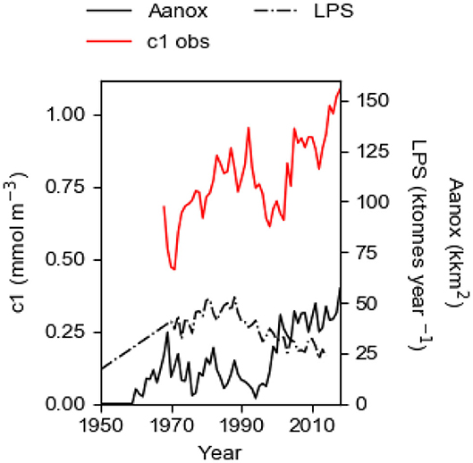
Figure 1. The observed winter surface concentration c1 (c1obs) in the 60 m thick surface layer of the Baltic proper 1968–2018; the land-based P source LPS 1950–2014; the area Aanox of anoxic bottoms 1950–2018. Data are described in the section Data.

The Baltic Sea is the second largest (373,000 km²) brackish water system in the world. The Baltic proper (251,000 km²), located south of the Gulf of Bothnia (Figure 2), is stratified by sea salt. The salinity of the typically 60-m-thick surface layer is ca 7 g kg⁻¹. A halocline separates the surface layer from the deepwater of salinity 12–20, with the highest salinity in the Arkona Basin closest to the mouth (e.g., Leppäranta and Myrberg, 2009). Only during seldom occurring so-called MBIs (Major Baltic Inflows), large amounts of high-saline water intrude through the shallow straits in the mouth (Matthäus and Franck, 1992; Gustafsson and Andersson, 2001; Stigebrandt et al., 2015b). The MBIs may exchange the deepest deepwater while smaller inflows are inserted (interleaved) higher up in the strongly stratified deepwater. The residence time of the deepest deepwater may be as large as 10 years, c.f. Supplementary Figure 1. The inflowing water from Kattegat plunges into the deepwater because the pycnocline in the Arkona Basin is below the shallow sills in Fehmarn Belt (15 m) and Öresund (8 m), c.f. Stigebrandt et al. (2015b). In the Baltic proper it proceeds as a dense bottom current toward the deep basins.

FIGURE 2

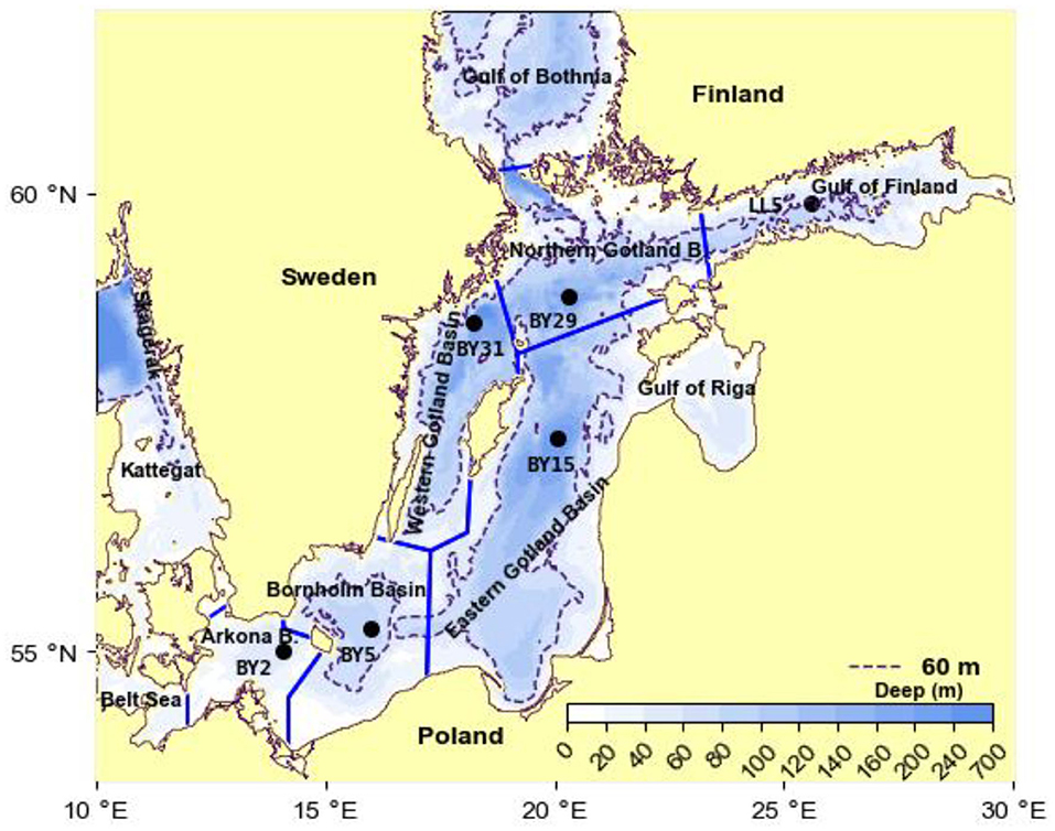
Figure 2. Topographic map of the Baltic proper showing the partition into deep basins. The Gulf of Riga is included in the Eastern Gotland Basin. Hydrographical data come from the stations marked in the map, see the section Data.

Due to extensive entrainment of overlying water into the dense bottom current, the highest salinity of the deepwater of the East Gotland Basin is only 12–13 despite the inflowing water from Kattegat may have salinities in the interval 20–30 (e.g., Stigebrandt et al., 2015b). Deepwater is transported to the surface layer by erosion during autumn and winter when the seasonal stratification in the surface layer has been eliminated and vertical convection reaches down to the halocline (e.g., Stigebrandt, 1985). Vertical convection and erosion of the upper part of the halocline thus reset the surface layer each winter. Vertical transport within the deepwater is due to breaking internal waves that by different mechanisms get much of their energy from the wind as inferred by Axell (1998). Tides are practically absent in the Baltic Sea. A large-scale tracer experiment shows that most of the diapycnal mixing in the deepwater takes place near the seabed (e.g., Holtermann et al., 2012).

The annual biological production of organic matter in the Baltic proper is determined by the P concentration c1 in the surface layer in winter, c.f. the seasonal cycles of PO₄ and DIN at the sea surface in Figure 3. When the spring bloom has exhausted the nitrogen nutrients, most of the phosphorus is left in the surface layer which makes possible extensive blooms of cyanobacteria that fixate elemental nitrogen (e.g., Olofsson et al., 2016). The importance of N-fixing species in the phytoplankton community has varied much in time as can be understood from the evolution of the NP ratio in the surface layer in winter (Figure 4). Decomposition of organic matter sinking out of the surface layer leads to oxygen consumption in the deepwater. Because turbulent vertical diffusion is obstructed by the strong vertical salinity stratification, the deepwater receives oxygen primarily by plunging inflows from the Kattegat. During a long period, the Baltic proper virtually lacked anoxic sulfidic deepwater (Fonselius and Valderrama, 2003; Savchuk et al., 2008). This period terminated at the end of the 1950s when oxygen demand outpaced supply and the deep basins became anoxic (Fonselius, 1962). The evolution since 1950 of the area Aanox of anoxic bottoms in the Baltic proper is shown in Figure 1.

FIGURE 3

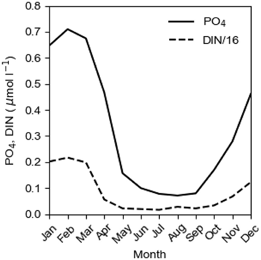
Figure 3. The mean seasonal cycles of PO4 and DIN/16 at the sea surface (0 m) at BY 15 in the East Gotland Basin in the period 2004–2018. Data from SMHI (2020).

FIGURE 4

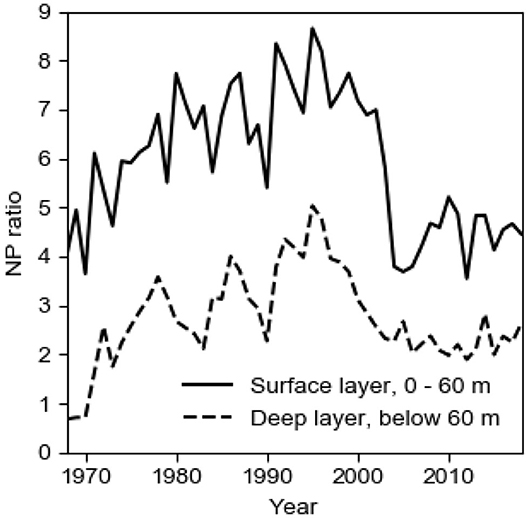
Figure 4. The long-term (1968–2018) evolution of the volume-weighted NP ratio, here (NO3 + NH4)/PO4 in winter in the 60 m thick surface layer and in the deepwater of the Baltic proper. Data from SMHI (2020).

The total phosphorus supply TPS to the Baltic proper water column has three components; the land-based supply LPS; the ocean supply OPS; the internal supply IPS from anoxic bottoms. Over long timescales, OPS can be considered as approximately constant ≈11 ktons year⁻¹ (Stigebrandt, 2018). LPS culminated in the 1980s and in 2014 it had about the same value as in the middle of the 1950s (Figure 1). Despite this, the observed winter surface layer P concentration c1 still increases (Figure 1). This runaway change of c1 cannot be explained as a simple response to the constant OPS and the declining LPS.

It is well-known that anoxic conditions in the bottom water permit an internal P source, IPS, from P storages in bottom sediments (Mortimer, 1941; Emeis et al., 2000; Gustafsson and Stigebrandt, 2007; Viktorsson et al., 2013; Stigebrandt et al., 2014; Hall et al., 2017; Sommer et al., 2017). The IPS in the Baltic proper has been described as a continuous reflux of P from the sediment during anoxic periods with hydrogen sulfide in the bottom waters (Emeis et al., 2000) although Gustafsson and Stigebrandt (2007) described the reflux as a single-dose release when the bottoms turned anoxic. Stigebrandt et al. (2014) suggested that IPS can be described as a continuous reflux proportional to the area Aanox of anoxic bottoms, thus IPS = fs·Aanox tons year⁻¹. This formulation implies that IPS vanishes in the Baltic proper when Aanox vanishes which is supported by Stigebrandt and Kalén (2013) and Viktorsson et al. (2013). Additional support is provided by Almroth-Rosell et al. (2015) who show that the P release rate from the sediment drastically decreased because of bottom water oxygenation by MBIs. Furthermore, sediment profile imagery showed that the deepwater sediment surface was oxygenated within a couple of months during natural oxygenation by a huge MBI (Rosenberg et al., 2016). This shows that the upward flux of hydrogen sulfide and ammonium, produced by anaerobic decomposition of organic matter in the deepwater sediments, is not large enough to hinder the formation of an oxic layer, containing P-adsorbing iron oxides, on top of the sediment when the bottom water is oxygenated. This contrasts with the situation in much more eutrophic lakes where the water/sediment interface remained anoxic during artificial oxygenation of the bottom water (Gächter and Wehli, 1998; Katsev and Dittrich, 2013). Much of the experience from highly eutrophicated lakes where restoration by oxygenation has failed is not applicable to the mildly eutrophicated salt-stratified Baltic proper (Stigebrandt, 2018).

Following Van Nes et al. (2016), the term tipping point may be used for any situation where accelerating change caused by a positive feedback drives the system to a new state. The tipping point is associated with the critical level at which a transition occurs. Once the threshold is passed, the dynamics of the system accelerate to cause a runaway change. The observed runaway change of c1 in the Baltic proper (Figure 1) suggests that there is a positive feedback between the observed state c1 and the total P supply TPS. The internal P supply IPS may provide such a positive feedback via its dependence on Aanox. In the beginning of the 1960s, when anoxia established in the deep basins of the Baltic proper, it was observed that large amounts of phosphorus accumulated in the anoxic deepwater (Fonselius, 1962). Apparently, the onset of anoxia turned on an IPS. The total P source TPS = LPS + OPS + IPS thereby obtained a component, IPS, that gives a positive feedback to the area of anoxic bottoms which is dependent on the production of organic matter in the surface layer and thereby controlled by c1.

Using the P budget model described in the section Model, we compute c1 (c1mod) for the period 1950–2014. The model is forced by known values of the external sources LPS and OPS. It is also forced by an internal source IPS, computed from IPS = fs·Aanox, where Aanox (km²) is known from observations and the parameter fs (tons km⁻² year⁻¹) is the specific P flux. The model is also forced by the internal and external sinks that are computed from c1·TRVF, where the parameter TRVF is the annual volume flow (km³ year⁻¹) carrying P to the sinks. Using the method of least squares, we determine the best estimate of the parameters TRVF and fs, giving the best correspondence between the modeled c1mod and the observed c1obs concentration of P in the surface layer. This application of the model is diagnostic, allowing us to show that it is necessary to include IPS in the P budget to explain the evolution of the observed state c1obs. We also use the model to discuss effects of shutting off IPS and reducing LPS with the aim to force TPS below its threshold value.

Materials and Methods

Data

Nutrient load compilations are carried out by all HELCOM countries to evaluate and quantify the amount of nutrients annually discharged from land into the sea. The data are obtained from national monitoring programs and reporting from industries and municipal water works. Data for the annual land-based supply of phosphorus LPS for the period 1970–2014 are obtained from Savchuk (2018) who use the best available estimates of external nutrient inputs from terrestrial sources (rivers, direct point, and diffusive sources) and the small atmospheric contribution. The supply for 1951–1969 is obtained by liner interpolation between the supply in 1950 from Savchuk et al. (2012) and the supply in 1970. For model purposes the water body is partitioned into two layers. The 60 m thick surface layer is thoroughly mixed down to the halocline each winter and below this is the lower layer. The observed P contents V1c1 and V2c2 in winter in the upper and lower layers of volumes V1 and V2, respectively, are volume weighted estimates obtained from vertical profiles of hydrographical data (of total phosphorus TP) from the main basins in the Baltic proper (Figure 2), obtained in the months December, January and February, from the hydrographical stations BY2, BY5, BY15, BY29, BY31 (ICES, 2020) and from station LL5 (SMHI, 2020) together with the hypsographic functions of the main basins, estimated from a hypsographic data base (Seifert et al., 2001). The observed time series of the P contents V1c1 and V2c2 describe the evolution of the system. The time series start 1968, before this year there are only sporadic P observations (see e.g., Stigebrandt, 2018). Examples of TP profiles from the East Gotland Basin are shown in Supplementary Figure 2.

The total area Aanox of anoxic bottoms in the Baltic proper for the period 1960–2018 are adopted from Hansson et al. (2019). In the period 1950–1959 there were apparently no anoxic bottoms, i.e., Aanox = 0 for these years. Hansson et al. (2019) use spatial interpolation of distributed oxygen profiles throughout the Baltic proper for the period August to October to determine Aanox which should be a robust approach. To investigate how well these values of Aanox may represent annual means, we computed both the annual oxygen mean and the oxygen mean for the period August to October in the deepwater of the Eastern, Northern and Western Gotland Basins. In the Eastern Basin there is practically no difference between the annual mean and the mean for the period August to October (Supplementary Table 2A), which means that there is almost no seasonal variation of the depth of the oxic-anoxic border. In the Northern and Western Basins (Supplementary Tables 2B,C, respectively), the oxic-anoxic border is about 7 m shallower in August to October than the annual mean. However, since the oxygen gradient at the oxic-anoxic border is quite weak, it is not obvious that an oxidized layer, stopping the IPS, will develop on top of an anoxic sediment when exposed to water with very low oxygen concentration during a fraction of a year. We therefore assume that the values of Aanox estimated by Hansson et al. (2019) may rather well represent annual means in the Baltic proper. In the model, annual values of IPS are computed from the values of Aanox. A constant value of OPS, 11 ktons year⁻¹ (Stigebrandt, 2018) is used for the whole period considered. This is in accordance with Rasmussen and Gustafsson (2003) who made a thorough analysis of nutrient pools and fluxes in the entrance to the Baltic Sea for the period 1974–1999, using a combination of hydrodynamic model results and observational data obtained in national monitoring programs. They found that the flux of TP to the Baltic proper, i.e., OPS, was quite stable at about 10 ktons year⁻¹ during the whole period. From their Figure 11 it seems that MBIs do not drive major inter-annual variability in OPS. The time series of c1, LPS, and Aanox are drawn in Figure 1. The observed values of LPS, Aanox, V1c1 and V2c2 are given in Supplementary Table 1.

In anoxic water in the Baltic proper, ammonia has been measured about 6 times more frequently than hydrogen sulfide as estimated from the hydrographical database Shark (SMHI, 2020). There is a quite good correlation between ammonium and hydrogen sulfide that we use to compute the concentration H₂S of hydrogen sulfide from the concentration NH₄ of ammonium as follows; H₂S = 4.18·NH₄ −5.89 if NH₄ > 1.41 and O₂ = 0; otherwise H₂S = 0. The oxygen debt is defined as the amount of oxygen needed to oxidize all hydrogen sulfide and ammonium present in the anoxic water column. The “concentration” of oxygen debt O2d(t,z,i) at the time t and depth z in sub-basin i, is computed as follows; O₂d(t,z,i) = 2·H₂S(t,z,i) + 2·NH₄(t,z,i) (mmol m⁻³), e.g., Reed et al. (2011). The total mass of the oxygen debt O₂debt(t,i) in the deepwater of sub-basin i at time t is obtained from the volume weighted vertical integral of O₂d(t,z,i).

Model

We apply a time-dependent model of the total amount of phosphorus P in the water column of the Baltic proper (Stigebrandt, 2018). The purpose of the model is to describe the long term evolution of the amount of P and this is best done by describing the state in winter when there is no primary production and the surface layer is reset by vertical mixing and entrainment of deepwater. In this type of model, the annual nutrient sink is related to the magnitude of the annual biological production which is assumed to be proportional to the surface layer winter concentration of the limiting nutrient (Vollenweider, 1969), which in the present case is P. Our model is a source-sink model of the type described by Vollenweider (1969) for lakes but compared to his model, our model is generalized in three ways namely; (i) introduction of time-dependence, (ii) introduction of an internal P source IPS from anoxic bottoms, (iii) introduction of two layers to account for effects of long residence time of the deepwater due to permanent salinity stratification. Essential features of the model are shown in Figure 5. Our model deals only with annual fluxes from sources and sinks of P and the balance of these fluxes that may lead to annual changes of the storages of P in the water column measured by changes of c1 and c2. There is also a seasonal internal cycling of P due to the production and decomposition of organic matter that does not give rise to annual changes of the P content of the water column and this is not resolved in the present model.

FIGURE 5

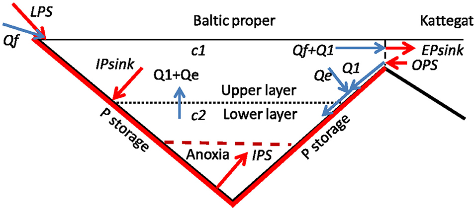
Figure 5. Essential features of the phosphorus model. Phosphorus fluxes from sources and to sinks are shown by red arrows and water fluxes by blue arrows. Red bottoms indicate possible locations of phosphorus storage. Qf, is freshwater supply; Q1, supply of Kattegat water; Qe, entrained flow from upper to lower layer; c1 (c2), mean winter P concentration in upper (lower) layer; LPS, the land-based P source; OPS, the ocean-based P source; IPS, the internal P source from anoxic bottoms; IPsink, the internal P sink; EPsink, the external P sink.

P will accumulate in the deepwater due to the several-years-long residence time of the deepwater in the Baltic proper, which is due to the salinity stratification. We account for this by the introduction of two layers in the model. In a two-layer context, the total amount of P in winter in the water column V$\overline{c}$ is composed of contributions from the upper and lower layers, thus

$\begin{array}{ll}V\overline{c}=V1·c1+V2·c2& (1)\end{array}$

Here $\overline{c}$ is the winter volume mean concentration of P in the water column and V is the volume of the Baltic proper and V1 (V2) the volume of the upper (lower) layer and c1 (c2) is the winter volume mean concentration in the upper (lower) layer. The upper layer encompasses the depth interval 0–60 m and it has the volume V1 = 10, 790 km³. The lower layer, beneath 60 m depth, has the volume V2 = 3,990 (km³) (Stigebrandt, 2018).

The total amount of P in the water column of the Baltic proper changes with time t as follows,

$\begin{array}{ll}V\frac{d\overline{c}}{dt}=TPS+TPsink& (2)\end{array}$

The term on the left side is the rate of change of P stored in the water column and the terms on the right side are the total P source TPS and the total P sink TPsink, respectively, acting on the water column of the Baltic proper. The time resolution dt in Equation (2) equals one year. TPS is the sum of the external sources EPS, i.e., the land-based source LPS and the ocean source OPS, and the internal source, IPS, thus

$\begin{array}{ll}TPS=EPS+IPS=LPS+OPS+IPS& (3)\end{array}$

The total sink TPsink has two components, the internal IPsink and the external EPsink. The internal sink IPsink is mainly located to the seabed and the external sink EPsink is due to export of P with surface water to Kattegat (the ocean). The annual removal rate of P from the surface layer to IPsink is related to the biological production and it is assumed to be proportional to c1 (Vollenweider, 1969). Since the photic zone in the Baltic proper is about 15 m, c.f. Kratzer et al. (2003), primary production should occur only in the surface layer. In the model also EPsink is proportional to c1 and to the outflow of surface water which equals the sum of the freshwater supply Qf and the inflow of ocean water (Wulff and Stigebrandt, 1989). TPsink can thus be written (Stigebrandt, 2018)

$\begin{array}{ll}TPsink=-c1·TRVF& (4)\end{array}$

Here the parameter TRVF is the Total Removal Volume Flux (km³ year⁻¹), carrying P to the internal and external sinks. In the present application we can estimate the parameter TRVF and thereby the total P sink TPsink. To estimate the sink components EPsink and IPsink, other methods must be used as briefly discussed later under section Results.

The nature of the internal P source IPS was briefly discussed in the Introduction. IPS is parameterized in the following way (Stigebrandt et al., 2014)

$\begin{array}{ll}IPS=fs·Aanox& (5)\end{array}$

Here Aanox (km²) is the area of anoxic bottoms in the Baltic proper and the parameter fs (tons km⁻² year⁻¹) the specific P flux from anoxic bottoms.

For simplicity, the following empirical relationship between c1 and c2 is introduced (Stigebrandt, 2018)

$\begin{array}{ll}V2·c2=\alpha ·V1·c1& (6)\end{array}$

Here the empirical parameter α equals the average ratio between the amounts of P in winter in the lower and upper layers, respectively. The value of α is determined by the residence time of the lower layer and α should be stable in time if the long-term mean vertical circulation does not change. Using this relationship simplifies the model and implies that we replace two equations, one for each layer, by one equation for the upper layer.

Using observed annual values of the total P content in winter in the upper and lowers layers, V1·c1 and V2·c2, the mean value of α is computed as follows,

$\begin{array}{ll}\alpha =\frac{{\displaystyle {\sum }_{i}V2c2(i)}}{{\displaystyle {\sum }_{i}V1c1(i)}}& (7)\end{array}$

Here the summation index i runs from 1968 to 2018 for which period interval P has been observed regularly in the Baltic proper, see the section Data. It is found that α for that period equals 1.15. Using Equation (6), it follows that as an average there are 15% more P in the lower than in the upper layer and c2 = 3.1·c1.

In the model, the ratio α occurs only in the combination K = (1 + α). It is therefore reasonable to investigate how K varies in time. The mean value of K = 2.15. Values vary between 1.73 and 2.74 (Figure 6) and the standard deviation of K = 0.20. With these modest variations of K, we conclude that it is reasonable to use a constant value of α to simplify the model.

FIGURE 6

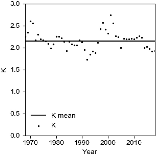
Figure 6. The evolution of K = (1 + α) in the period 1968–2018.

Using Equations (1), (4), and (6), we can rewrite Equation (2) as follows

$\begin{array}{ll}\frac{dc1}{dt}=\frac{TPS-c1·TRVF}{K·V1}& (8)\end{array}$

From this follows that the lower layer, through the parameter α, increases the inertia and thus the spin-up time of the system. Equation (8) shows that dc1/dt > 0 when the total source TPS is greater than the total sink c1·TRVF and vice versa. In the present paper we integrate Equation (8) to compute the evolution of the concentration c1 in the surface layer, starting from 1950.

The equilibrium concentration c1e in the surface layer in winter occurs under steady-state (equilibrium) conditions when dc1/dt = 0. For this case Equation (8) gives

$\begin{array}{ll}c1e=\frac{TPS}{TRVF}& (9)\end{array}$

The equilibrium concentration c1e is thus proportional to the total P supply TPS to the water column of the Baltic proper. Please note that the ratio α between the amounts of P in the lower and upper layers does not influence the equilibrium concentration c1e. This is easily realized because the sink is proportional to the surface concentration c1, see Equation (4).

Analytical solutions of the time-dependent model for two cases, Case 1 and Case 2 were discussed by Stigebrandt (2018). Case 2 has the same vertical stratification as the model in the present paper. In Case 1, the salt stratification, and thereby the lower layer, is absent and there is thus only one layer of volume V = V1 + V2. This situation has not been observed in the Baltic proper and should therefore be quite unusual. However, when it happens the deep bottoms are oxygenated by the surface layer, which is well-oxygenated through direct contact with the atmosphere at the sea surface, and this should be an efficient way for “self-restoration” of the Baltic proper (Stigebrandt, 2018). This is further discussed in the section Self-Restoration of Historic Episodes of Eutrophication in the Baltic Proper.

For Case 2, the two-layer case, Stigebrandt (2018) showed that the e-folding time T equals

$\begin{array}{ll}T=K\frac{V1}{TRVF}& (10)\end{array}$

The time-scale T is inversely proportional to the total sink flux TRVF. The existence of a lower layer (i.e., K > 1) increases T, and thereby the time to reach equilibrium. Please note that T is independent of the magnitude of the P source TPS.

Stigebrandt (2018) introduced the restoration time TR, defined as the time it takes to achieve 95% of the expected concentration change due to an instantaneous change of TPS, which is approximately described by the following relationship

$\begin{array}{ll}TR=3T& (11)\end{array}$

In the present application of the model, TRVF in Equation (4) and fs in Equation (5) are unknown parameters that govern the total sink and the internal source, respectively. We apply the least squares method to determine the best estimate of TRVF and fs. The best fit in the least-squares sense minimizes the sum of squared residual Ssr. The residual is the difference between the observed value c1obs and the value c1mod computed by the model. Ssr(TRVF, fs) is defined as follows

$\begin{array}{ll}Ssr(TRVF,fs)={\displaystyle \sum _{i=1}^N}{(c1obs(i)-c1mod(i))}^2& (12)\end{array}$

Here N is the length (number of years) of the observational series c1obs. In the present application N equals 47 years (1968–2014). We compute Ssr(TRVF, fs) for wide ranges in the parameter space (TRVF, fs). The best estimate is given by the pair of values of TRVF, fs that gives the least value of the sum of squared residual Ssr(TRVF, fs).

Results

Estimation of the Parameters TRVF and fs

We first apply the method of least squares to find the pair of values of the parameters TRVF and fs, regulating the internal and external sinks and the internal source, respectively, that gives the best model description c1mod of the observations c1obs. Using the time series of LPS and Aanox and the constant value of OPS, see the section Data, and the initial value c1i = 0.20 mmol m⁻³ at the start of the computations in 1950, Equation (8) was integrated to compute the year to year evolution of the P concentration c1mod in the surface layer in winter in the Baltic proper in the period 1950–2014. We repeated the computations for values of TRVF from 1,800 to 5,000 (km³ year⁻¹) and values of fs from 0 to 3 (tons km⁻² year⁻¹). We found that the least value of the sum of squared residual Ssr(TRVF, fs), defined by Equation (12), equals 0.50 (mmol m⁻³)². It occurs for the pair TRVF = 3,000 (km³ year⁻¹) and fs=1.22 (tons km⁻² year⁻¹). Before plotting Ssr(TRVF, fs) in Figure 7, we normalized by division with the least value, i.e., 0.50. It can be seen (Figure 7) that good solutions (i.e., small values of Ssr) are obtained for an elongated, trench-formed area of the parameter space, clearly showing that TRVF and fs are dependent, a greater source (fs) requires a greater sink (TRVF) and vice versa. However, as further discussed in the section The Baltic Proper Response to IPS, it is not possible to obtain the runaway behavior shown by c1obs from a model lacking an internal source IPS, i.e., with fs = 0.

FIGURE 7

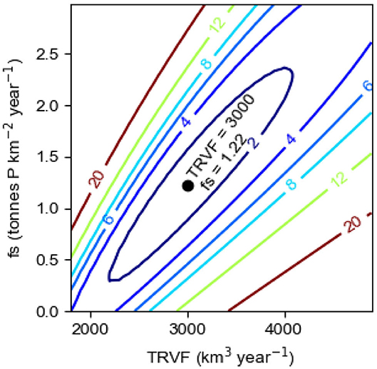
Figure 7. Model results showing the normalized sum of the squared residual Ssr(TRVF, fs), see Equation (12), in the parameter space 1,800 ≤ TRVF ≤ 5,000, 0 ≤ fs ≤ 3. The least value of Ssr(TRVF, fs) occurs for TRVF = 3,000 km³ year⁻¹ and fs = 1.22 tons km⁻² year⁻¹.

The analysis gives the total sink flow TRVF = 3,000 km³ year⁻¹. This solution does not depend upon the partition between different kinds of sinks. If needed, partition of the total sink into the two main sink components, IPsink and EPsink, must be performed using other methods. The part of TRVF belonging to the external sink EPsink equals 720 km³ year⁻¹ according to Wulff and Stigebrandt (1989). The part of TRVF belonging to the internal sink, IPsink, should then be 2,280 km³ year⁻¹ and the (fix) ratio between the external and internal sinks, EPsink/IPsink, equals 0.32. The external sink by export to the ocean (Kattegat) is responsible for 720/3,000 = 24% of the total sink.

Initial Value and Spin-Up Time

Due to lack of observational data, the initial value c1i, in 1950, is not known. We run the model with c1i equal to 0.15, 0.20, and 0.25 mmol m⁻³ to study the importance of the initial value for the result of the computations. From Equation (10) and using K = 2.15 and TRVF = 3,000 km³ year⁻¹, one finds that the time constant T of the system is about 7.7 years (e-folding time). 95% of the change due to an instantaneous change of c1 should have occurred after the time TR = 3T, see Equation (11). The curves for the runs with different initial concentrations converge (Figure 8), showing that the memory of the chosen initial value is almost lost after about 23 years as predicted by Equation (11). We can also call this time the spin-up time. This spin-up time implies that our estimate of the best fit of TRVF and fs in the previous section, starting the computations in 1950 and using data on c1mod beginning in 1968, should be very little influenced by the chosen initial value c1i.

FIGURE 8

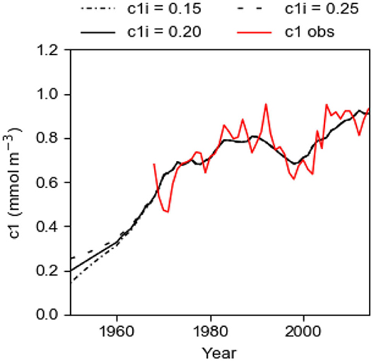
Figure 8. Computational results c1mod from the best fit model with fs = 1.22 tons km⁻² year⁻¹ and TRVF = 3,000 km³ year⁻¹. Three different initial concentrations c1i were applied. The graphs show the computed concentration c1mod 1950–2014 (black lines) and the observed concentration c1obs 1968–2014 (red line) of phosphorus in the surface layer in winter.

Model Performance

The long-term evolution of c1 computed by the model for the best fit case, i.e., with TRVF = 3,000 km³ year⁻¹ and fs = 1.22 tons km⁻² year⁻¹, mimics the observed concentration quite well and this comparison provides a successful test of the model (Figure 8). It should be noted that the large reduction of the land-based P source LPS after the 1980s is not accompanied by a corresponding decrease of c1obs (Figure 1). On the contrary, c1obs shows an increasing runaway change after the 1990s, like the evolution of Aanox and IPS. We conclude that the favorable comparison between c1mod and c1obs (Figure 8) shows that the internal P source IPS as estimated in the present paper is of decisive importance for the successful model description of the evolution of c1 in the anoxic Baltic proper, see also the section The Baltic Proper Response to IPS.

Evolution of Sinks and Sources

The evolution of the total sink TPsink and the total source TPS and its components LPS, OPS and IPS are shown in Figure 9 for the best fit case displayed in Figure 8. As from about year 2000, the internal source IPS is about 50 ktons year⁻¹ which is about two times larger than present time LPS (Figure 9). The evolution of IPS caused TPS to increase from about 1997 which explains the obvious runaway change of c1 after the end of the 1990s. For comparison, we note that the internal sink IPsink (=2,280/3,000 TPsink) is about 50 ktons year⁻¹ after year 2000. The curve IPsink + IPS (red) shows that there was a net growth (i.e., negative values) of the internal storage before year 2000, which thereafter has ceased (Figure 9).

FIGURE 9

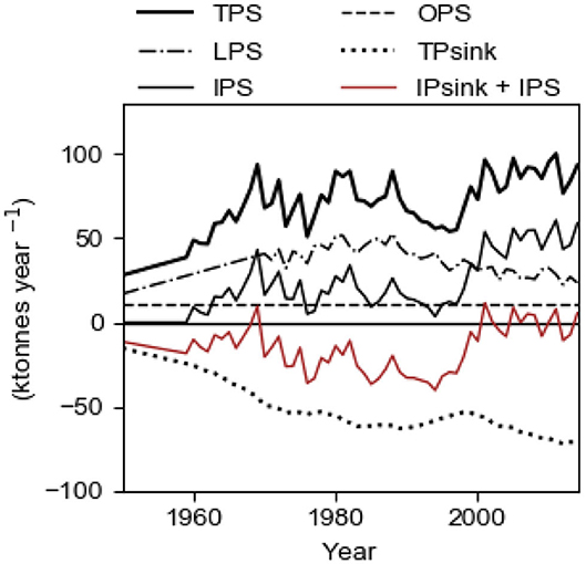
Figure 9. Sources and sinks in the Baltic proper in the period 1950–2014. Computational results from the model with fs = 1.22 tons km⁻² year⁻¹ and TRVF = 3,000 km³ year⁻¹. LPS, OPS, and Aanox are input data. TPS equals LPS + OPS + IPS and TPsink = IPsink + EPsink and EPsink ≈ 0.24·TPsink. The curve IPsink + OPS shows the net growth (negative values in the graph) of the internal storage of P.

We recall that OPS, the estimated oceanic import, equals 11 ktons year⁻¹. The export to the ocean EPsink = 720/3,000 ·TPsink, increases with c1 and before about 1965, OPS was greater than EPsink implying that the Baltic proper had a net import of P from the ocean. Thereafter the Baltic proper has had a net export to the ocean and the present time net export (EPsink – OPS) is about 6 ktons year⁻¹.

The Baltic Proper Response to IPS

To further elucidate the effect of IPS, we compare the best fit curve c1mod (with TRVF = 3,000; fs = 1.22), which rather well describes the evolution of c1obs, and the curve c1hyp (TRVF = 3,100: fs = 0) which is the hypothetical evolution of c1 if Aanox = 0 and IPS = 0 for the period 1950–2014 (Figure 10). The curve c1hyp thus shows the hypothetical response of the Baltic proper in the absence of IPS so that the total P supply equals LPS plus OPS. The stippled area between the curves c1mod and c1hyp shows the contribution by the internal supply IPS (Figure 10). The role of IPS increased rapidly at the end of the 1990s and at the present, IPS is evidently a major driver of the eutrophication of the Baltic proper. This is also evident from the evolution of LPS, OPS, and IPS (Figure 9) as discussed above. Apparently, the IPS has severely boosted and perpetuated the eutrophication of the Baltic proper. Interestingly, IPS was relatively large already during several years in the period 1963–1988 (Figure 9) but to the best of the authors' knowledge, the effect of IPS in that period has not earlier been quantified. However, Wulff and Stigebrandt (1989) concluded from the results of their Baltic Sea P-budget modeling, using data from the 1970s, that there seemed to be a contribution from an internal P source, but they did not estimate its magnitude.

FIGURE 10

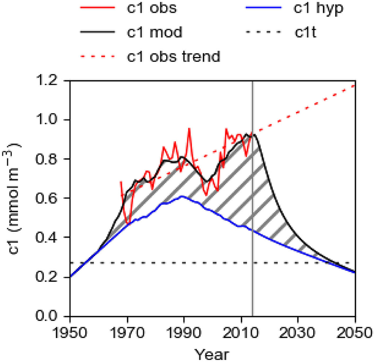
Figure 10. Computational results from the best fit model for the period 1950–2014 (2014 marked by vertical line) with the internal source IPS turned on (c1mod with fs = 1.22) and turned off (c1hyp with fs = 0, blue line). Also shown is the observed c1obs (red line) for the period 1968–2014. The shaded area shows the estimated contribution to c1 by the IPS. In the computation for the period 2015–2050, IPS is shut off (full-drawn black line). The blue line shows the computed hypothetical evolution c1hyp with IPS shut off for the whole period 1950–2050. Also shown is the linear trend c1obstrend of c1obs (determined by the least square method for the period 1968–2018) which is extrapolated to 2050, and the threshold concentration c1t = 0.27 mmol m⁻³.

The computed curves c1mod and c1hyp (Figure 10) are identical from the start in 1950 to the onset of deepwater anoxia in 1960. Anoxia occurred because c1 increased, due to increasing LPS, and passed the threshold value c1t making the deepwater oxygen consumption larger than the oxygen supply. The system passed a tipping point when anoxic bottoms established and turned on the IPS which affects c1mod, but not c1hyp, and the curves took different routes. The existence of anoxic bottoms and the accompanying IPS means that the system obtains a positive P feedback. Due to the typically decadal-long residence time of the deepwater, the threshold value c1t was likely passed in the second half of the 1950s. According to Stigebrandt (2018), c1 was about 0.27 mmol m⁻³ in 1958 and we adopt this value for c1t. We estimate that TPS was about 36 ktons year⁻¹ when the threshold value c1t was passed (Figure 9). This value of TPS should thus be the threshold value TPSt for the total P supply. Since IPS was zero before the tipping point was crossed, the threshold value of the land-based supply LPSt (=TPSt – OPS) should be about 25 ktons year⁻¹. For larger supplies we expect that c1 > c1t and deepwater anoxia may develop and thereby turn on an IPS in the Baltic proper.

Reversing Eutrophication and Crossing the Tipping Point by Shutting Off IPS

To predict the future evolution of c1, the unknown area of anoxic bottoms Aanox must be predicted. Normally, this would require the coupling of an oxygen model to our P model. However, for the special case Aanox = 0 due to oxygenation of the bottom water there is no need to predict Aanox and we may use the present model without a coupled oxygen model. We thus use our model to predict the response of c1 to shutting off IPS by keeping all bottoms oxygenated. For these computations, the oxygenation starts in 2015 and we set Aanox(2015) = Aanox(2014)/2. For 2016 and the subsequent years we set Aanox = 0. The LPS time series is extrapolated to 2050 by assuming an annual reduction of LPS by 0.5 ktons year⁻¹ for the subsequent years from the value in 2014 which is consistent with the Baltic Sea Action Plan (HELCOM, 2007).

The result of the computation for the period 2014–2050 is shown on the right-hand-side of Figure 10. The computed concentration c1mod decreases drastically in an exponential way when IPS is shut off and approaches asymptotically the curve c1hyp. The timescale of this adjustment process is given by the restoration time RT, see Equation (11), which we above estimated to about 23 years. At about 2044, c1mod is predicted to have declined below the threshold concentration c1t implying that the Baltic proper has been restored to a state below the tipping point like that in the early 1950s.

During the oxygenation process, most of the P that is removed from the water column (about 500 ktons) will end up in the internal sink IPsink. The export EPsink of P to the Kattegat (ocean) by the export of surface water will decrease rapidly since the export is proportional to c1. In the restored state, there will be a net import of P (OPS + EPsink > 0) from Kattegat, like before about 1965 as discussed above. In the simulation, LPS is reduced by 0.5 ktons year⁻¹ for the whole period after 2014, see the section Data, and therefore c1hyp is slowly decreasing until the end of the simulation in 2050 (Figure 10).

Discussion and Concluding Remarks

The specific flux fs of P from anoxic bottoms estimated in the present paper, 1.22 tons km⁻² year⁻¹, is only about 53% of the flux estimated by Stigebrandt et al. (2014) from a P budget using observational data from only 2 years (1980 and 2005). The fs-value computed in the present paper should be the correct value to use because (i) it is derived using a budget model and the least squares method and 47 years of observational data describing the state c1obs of the Baltic proper, (ii) the model describes quite well the runaway evolution of c1obs during the last decades despite a simultaneously halved LPS. The value of fs estimated in this way represents the temporal average over many (47) years and the spatial average across the model area.

The results from our model may be compared to results obtained from more complex biogeochemical models. Almroth-Rosell et al. (2015) use a detailed biogeochemical model coupled to a high resolution hydrodynamical model. The oxygen penetration in the sediment is computed using 7 empirical constants and the detailed P model contains 14 empirical constants. Simulation of the Baltic proper in the period 1980–2008 shows that compared to observations the modeled oxygen and phosphate concentrations below the halocline are too high and too low, respectively, with largest differences closest to the bottom. They estimated the mean transport of P from anoxic bottoms (i.e., the IPS) for the period 1980–2008 to a about 77 ktons year⁻¹. For the same period the present model computes a mean IPS of only about 25 ktons year⁻¹.

In the section Results, it was shown that the internal P supply IPS from anoxic bottoms gives a positive feedback that boosts and perpetuates eutrophication in the Baltic proper. This self-amplifying process of eutrophication starts when the total P supply TPS exceeds the threshold value TPSt so that anoxic bottoms are created, which obviously is the tipping point of the system, c.f. Van Nes et al. (2016). The discovery that the Baltic proper eutrophication system has passed a tipping point and that IPS is a decisive component that now is the major driver of eutrophication (Figure 9) calls for a paradigm shift for the management strategy for the Baltic Sea that should include sea-based measures to reduce eutrophication.

Self-amplifying eutrophication due to IPS should occur also in other permanently stratified basins with anoxic deepwater. Provided there are long time series of the P content in the water body, and of the external P sources, and of the area Aanox of anoxic bottoms, the magnitude of IPS might be estimated using the same kind of regression analysis as used in the present paper.

Anoxia Boosts Eutrophication in Two Ways

Hydrogen sulfide and ammonium from anaerobic decomposition of organic matter in the sediment may accumulate in anoxic bottom water and thereby contribute to an oxygen debt O2debt as defined in the section Data. The debt may cause oxygen loss (two moles of oxygen for each mole of hydrogen sulfide and ammonium, respectively) in inflowing new deepwater when this entrains old deepwater with oxygen debt. This should occur geographically in the Bornholm Basin and in the adjacent part of the southern East Gotland Basin (EGB) (e.g., Stigebrandt et al., 2015b). This phenomenon was discussed by Fonselius (1970) who concluded that the Baltic proper no longer in a natural way can recover from what he called “the hydrogen sulfide shocks.” It should be noted that O2debt in EGB shows a strong increasing trend, starting from small values in the 1970s (Figure 11), which should imply co-occurring decreasing trends in both the oxygen supply and the oxygen content of the deepwater in the EGB. The deepwater oxygen debt should be a more important factor for the observed decrease of the oxygen content in the deepwater of the Baltic proper than the reduction of oxygen saturation due to a higher temperature, which only may explain about 3% reduction of oxygen content per degree Celsius temperature increase, c.f. Carstensen et al. (2014).

FIGURE 11

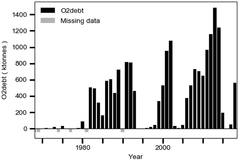
Figure 11. The evolution of the oxygen debt O2debt in the East Gotland Basin computed from hydrographical data from station BY15 in the period 1968–2018 as described in the section Data.

As shown by the model in the present paper, anoxia and the accompanying IPS leads to increased c1 and biological production, which increases the oxygen demand in the deepwater. As discussed above, an oxygen debt O2debt in anoxic deepwater leads to reduced oxygen supply to the deepwater. Thus, anoxia both increases the demand and reduces the supply of oxygen to the deepwater, which tends to increase the oxygen debt in the deepwater and the area of anoxic bottoms and thereby boost IPS and eutrophication.

Self-Restoration of Historic Episodes of Eutrophication in the Baltic Proper

The threshold value TPSt of the total P supply depends on the rate of oxygen supply to the deepwater. Since the rate of oxygen supply to the deepwater of the Baltic proper varies in time, TPSt should be defined for a period of minimum supply of oxygen like that in the 1950s caused by the unrivaled salty inflow in 1951 (Fonselius and Valderrama, 2003). The establishment of extremely strong vertical stratification, like in 1951, will likely prevent oxygen supply to the deep parts of the basins for many consecutive years, which may cause anoxia and thereby IPS and a runaway change of c1 that can explain the emergency of historic periods of eutrophication in the Baltic proper (c.f. Bianchi et al., 2000). The ending of historic periods of eutrophication by episodes of self-restoration was discussed by Stigebrandt (2018). He suggested that the deep bottoms may be oxygenated by contact with the well-oxygenated surface water during sufficiently long episodes of large-amplitude halocline deepening that eliminate the vertical stratification and Aanox and IPS. When this occurs, c1 should decrease as predicted during oxygenation of deepwater bottoms (Figure 10). This scenario is supported by sediment observations of rapid termination of historic anoxic periods (Jilbert and Slomp, 2013). The statistical recurrence time of decadal-long episodes of large-amplitude halocline deepening may be many hundred years (work in progress).

Business-as-Usual

The present management strategy to reduce the eutrophication of the Baltic Sea, here called the “business-as-usual” scenario, is to reduce LPS according to the Baltic Sea Action Plan (HELCOM, 2007). The LPS has been successfully reduced since the 1980s (Figure 1; HELCOM, 2017) but this has neither led to reduced c1 nor to reduced area Aanox of anoxic bottoms (Figure 1). The reason for this is the positive feedback provided by the IPS as shown in the present paper. Since both the area Aanox of anoxic bottoms (Figure 1) and the oxygen debt O2debt in EGB (Figure 11) show increasing trends, it is consistent to assume that the self-amplifying eutrophication process driven by IPS from anoxic bottoms will continue with an expected modest rate of increase of c1, as also suggested by the extrapolated linear trend c1obstrend of the observations c1obs (Figure 10).

In the “business-as-usual” scenario one may expect increased annual production of cyanobacteria (Vahtera et al., 2007) and the neurotoxin BMAA (Jonasson et al., 2010). One may also expect still worsened conditions for the Baltic cod which has experienced a strong decline in mean body conditions linked to hypoxia exposure (Limburg and Casini, 2019). An increased c1 would also lead to ecological changes at shallower water depths including all coastal and most inshore areas, c.f. Elmgren (1989).

Sea-Based Measures Stopping the IPS Might Restore the Baltic Sea

Since IPS from anoxic bottoms is the present time major driver of the eutrophication, as shown in the present paper, it follows that measures to eliminate IPS should be included in the management strategy to reduce the eutrophication of the Baltic proper. In the model simulation for the period 2015–2050 (Figure 10), IPS is shut off by natural or engineered sea-based deepwater oxygenation removing bottom anoxia. The Baltic proper might be restored to a state similar to that prevailing before the crossing of the tipping point in the end of the 1950s. The engineered oxygenation can be turned off when c1 < c1t and TPS has been pushed below the threshold value TPSt which means that LPS should be less than LPSt, estimated to about 25 ktons year⁻¹ in the section The Baltic Proper Response to IPS. The measures undertaken on land until now to reduce LPS have been successful (Figure 1) and LPS should be far below LPSt when c1 falls below c1t. It should be stressed that all bottoms must be kept oxic during the whole restoration process so that IPS vanishes. If some bottoms remain anoxic, the IPS from these may make TPS greater than TPSt so that restoration would fail. When the deep bottoms have been oxidized and colonized by animals, there might possibly be an IPS of a different kind caused by animal decomposition of organic matter stored in the bottom sediment as discussed in Stigebrandt (2018). However, this should not jeopardize the restoration if TPS < TPSt.

Only systems fulfilling the following requirements can be restored by sustained oxygenation of the bottoms: (i) the IPS from anoxic bottoms provides a major P loading component and (ii) LPS can be reduced to less than LPSt. The anoxic By Fjord, for instance, that was oxygenated during a pilot experiment (Stigebrandt et al., 2015a), does not belong to this category and, as expected, a few years after the end of the experiment the fjord had returned to a state similar to that before the experiment.

The first proposal to oxygenate the deepwater of the Baltic proper to reduce c1 was presented by Stigebrandt and Gustafsson (2007) who suggested that the cool and almost oxygen saturated so-called winter water, located above the halocline, should be mixed into the deepwater by pumping. This method was applied in a theoretical experiment of oxygenation of the Bornholm Basin (Figure 2), which shows that the deepwater may be kept well-oxygenated, of great benefit for e.g., the Baltic Sea cod, by mixing about 1,000 m³s⁻¹ of winter water into the deepwater (Stigebrandt et al., 2015b). Several environmental effects of pumping and mixing 2 m³ s⁻¹ of well-oxygenated surface water of often low salinity into the deepwater were investigated in a pilot experiment in the small anoxic By Fjord (Stigebrandt et al., 2015a). Among others, it was found that the top of the anoxic sediment was oxygenated and colonized within about 1 year. A rapid decrease of sediment phosphate fluxes when anoxic bottoms in eutrophic estuaries were oxygenated by engineered destratification and reaeration was reported by Harris et al. (2015). Different methods to alleviate bottom layer hypoxia through induced downwelling on shallow stratified shelves have recently been described by Koweek et al. (2020) and Xiao et al. (2018).

A recent publication investigating the legal aspects of sea-based engineering measures to combat the eutrophication of the Baltic Sea concludes that the legality of any sea-based measure depends on the risks they present balanced against their benefits (Ringbom et al., 2019). The benefit of a restored Baltic Sea is huge; estimates suggest that the present deteriorated state of the Baltic proper reduces the annual value of Baltic Sea services to mankind by about 32 milliards EUR (Boston Consulting Group, 2013). The annual cost to oxygenate the deep basins by mixing well-oxygenated winter water into the denser deepwater as described in Stigebrandt and Kalén (2013) and Stigebrandt et al. (2015b) should be of the order of 1% of the estimated benefit. The ecological response in the whole water mass to the reduced P concentration c1 in the surface layer, and risks, benefits, and costs should be thoroughly described in an Environmental Impact Assessment.

Important Research Questions

The specific internal P source fs = 1.22 tons km⁻² year⁻¹ from anoxic bottoms and the total sink flow TRVF=3,000 km³ year⁻¹, estimated in the present paper are temporal system averages, determined using 47 years of data on input and response of the Baltic proper to the P loading. There are numerous in situ observations of the flux of P between the seabed and the bottom water (e.g., Viktorsson et al., 2013; Hall et al., 2017; Sommer et al., 2017). These fluxes may obtain contributions from both internal storages (the internal source) and decomposition of fresh organic matter, the latter is not included in our sink-source P-budget model. So far, there are no published estimates of temporal and spatial Baltic proper averages of the reflux from internal storages, based on in situ observations, that may be compared to our value fs = 1.22 tons km⁻² year⁻¹.

The values of fs and TRVF estimated in the present paper can be used to constrain P budgets in more complex models. The total sink flow TRVF is composed of sink flows to internal sinks IPsink and to external sinks EPsink by export to external areas. According to the present model, the total P sink after year 2000, for instance, equals about 65 ktons year⁻¹ (Figure 9). With this constriction on the total sink, it would be very interesting to set up a table of the magnitude of the partial P sinks, including sinks in oxic and anoxic bottoms, sinks due to changing masses of living biota, sinks due to fish brought on land and stranded algae, and sinks due to export to Kattegat and the Bothnian Sea.

Finally, more research is needed to describe the nature of the internal P source IPS from anoxic bottoms that still is only vaguely known, e.g., Emeis et al. (2000), Gustafsson and Stigebrandt (2007), Viktorsson et al. (2013), Stigebrandt et al. (2014), Hall et al. (2017), Sommer et al. (2017). The fs-value estimated in the present paper includes all internal sources and cannot differentiate between continuous and short-term single-dose releases from oxic bottoms that turn anoxic. As a first step toward learning more about IPS it would be important if the relative magnitudes of these two types of contributions to IPS could be estimated.

Data Availability Statement

The original contributions presented in the study are included in the article/Supplementary Materials, further inquiries can be directed to the corresponding author.

Author Contributions

AS designed the study and wrote the manuscript. AA prepared data, made the calculations, prepared the figures. AS and AA discussed the results. All authors contributed to the article and approved the submitted version.

Funding

This work was supported by a grant, Dnr 2000–2018, to AS from the Swedish Agency for Marine and Water Management.

Conflict of Interest

The authors declare that the research was conducted in the absence of any commercial or financial relationships that could be construed as a potential conflict of interest.

Acknowledgments

The reviews led to improvements of the quality of the paper.

Supplementary Material

The Supplementary Material for this article can be found online at: https://www.frontiersin.org/articles/10.3389/fmars.2020.572994/full#supplementary-material

References

Almroth-Rosell, E., Eilola, K., Kuznetzov, I., Hall, P. O. J., and Meier, H. E. (2015). A new approach to model oxygen dependent benthic phosphate fluxes in the Baltic Sea. J. Marine Syst. 144, 127–141. doi: 10.1016/j.jmarsys.2014.11.007

CrossRef Full Text | Google Scholar

Axell, L. (1998). On the variability of Baltic Sea deepwater mixing. J. Geophys. Res. 103, 21667–21682. doi: 10.1029/98JC01714

CrossRef Full Text | Google Scholar

Bianchi, T. S., Engelhaupt, E., Westman, P., Andrén, T., Rolff, C., and Elmgren, R. (2000). Cyanobacterial blooms in the Baltic Sea: natural or human-induced? Limnol. Oceanogr. 45, 716–726. doi: 10.4319/lo.2000.45.3.0716

CrossRef Full Text | Google Scholar

Boston Consulting Group (2013). Turning adversity into opportunity. a business plan for the Baltic Sea. Commissioned by WWF, 1–32.

Google Scholar

Carstensen, J., Andersen, J. H., Gustafsson, B. G., and Conley, D. J. (2014). Deoxygenation of the Baltic Sea during the last century. Proc. Natl. Acad. Sci. U.S.A. 111, 5628–33. doi: 10.1073/pnas.1323156111

PubMed Abstract | CrossRef Full Text | Google Scholar

Elmgren, R. (1989). Man's impact on the ecosystem of the Baltic Sea: energy flows today and at the turn of the century. Ambio 18, 326–332.

Google Scholar

Emeis, K.-C., Struck, U., Leipe, T., Pollehne, F., Kunzendorf, H., and Christiansen, C. (2000). Changes in the C, N, P burial rates in some Baltic Sea sediments over the last 150 years—relevance to P regeneration rates and the phosphorus cycle. Marine Geol. 167, 43–59. doi: 10.1016/S0025-3227(00)00015-3

CrossRef Full Text | Google Scholar

Fonselius, S. H. (1962). Hydrography of the Baltic deep basins. Rep. Fishery Board Sweden 13:41.

Fonselius, S. H. (1970). On the stagnation and recent turnover of the water in the Baltic. Tellus 22, 533–544. doi: 10.3402/tellusa.v22i5.10248

CrossRef Full Text | Google Scholar

Fonselius, S. H., and Valderrama, J. (2003). One hundred years of hydrographic measurements in the Baltic Sea. J. Sea Res. 49, 229–241. doi: 10.1016/S1385-1101(03)00035-2

CrossRef Full Text | Google Scholar

Gächter, R., and Wehli, B. (1998). Ten years of artificial mixing and oxygenation: no effect on the internal phosphorus loading of two eutrophic lakes. Environ. Sci. Technol. 32, 3659–3665. doi: 10.1021/es980418l

CrossRef Full Text | Google Scholar

Gustafsson, B. G., and Andersson, H. C. (2001). Modeling the exchange of the Baltic Sea from the meridional atmospheric pressure difference across the North Sea. J. Geophys. Res. Oceans 106, 19731–19744. doi: 10.1029/2000JC000593

CrossRef Full Text | Google Scholar

Gustafsson, B. G., and Stigebrandt, A. (2007). Dynamics of nutrients and oxygen/hydrogen sulfide in the Baltic Sea deep water. J. Geophys. Res. Biogeosci. 112:G02023. doi: 10.1029/2006JG000304

CrossRef Full Text | Google Scholar

Hall, P. O. J., Almroth-Rosell, E., Bonaglia, S., Dale, A. W., Hylén, A., Kononets, M., et al. (2017). Influence of natural oxygenation of Baltic proper deep water on benthic recycling and removal of phosphorus, nitrogen, silicon and carbon. Front. Marine Sci. 4:27. doi: 10.3389/fmars.2017.00027

CrossRef Full Text | Google Scholar

Hansson, M., Viktorsson, L., and Andersson, L. (2019). Oxygen survey in the Baltic Sea 2018-extent of Anoxia and Hypoxia, 1960-2018. SMHI Swedish Meteorological and Hydrological Institute. Report Oceanography No. 65, 11 pp + 2 Appendices.

Google Scholar

Harris, L. A., Hodgkins, C. L. S., Day, M. C., Austin, D., Testa, J. W., and Boynton, W. (2015). Optimizing recovery of eutrophic estuaries: impact of destratification and re-aeration on nutrient and dissolved oxygen dynamics. Ecol. Eng. 75, 470–483. doi: 10.1016/j.ecoleng.2014.11.028

CrossRef Full Text | Google Scholar

HELCOM (2007). “HELCOM Baltic Sea action plan,” in HELCOM Ministerial Meeting in Krakow (Krakow), 101 pp.

Google Scholar

HELCOM (2017). The integrated assessment of eutrophication - supplementary report to the first version of the HELCOM ‘State of the Baltic Sea report’.

Holtermann, P. L., Umlauf, L., Tanhua, T., Schmale, O., Rehder, G., and Waniek, J. J. (2012). The Baltic Sea tracer release experiment: 1. Mixing rates. J. Geophys. Res. 117:C01021. doi: 10.1029/2011JC007439

CrossRef Full Text | Google Scholar

ICES (2020). Available online at: https://ocean.ices.dk/HydChem/HydChem.aspx?plot=yes (accessed September 10, 2020).

Jilbert, T., and Slomp, C. P. (2013). Rapid high-amplitude variability in the Baltic Sea hypoxia during the Holocene. Geology 41, 1183–1186. doi: 10.1130/G34804.1

CrossRef Full Text | Google Scholar

Jonasson, S., Eriksson, J., Berntzon, L., Spáčil, Z., Ilag, L. L., Ronnevi, L.-O., et al. (2010). Transfer of a cyanobacterial neurotoxin within a temperate aquatic ecosystem suggests pathways for human exposure. Proc. Natl. Acad. Sci. U.S.A. 107, 9252–9257. doi: 10.1073/pnas.0914417107

PubMed Abstract | CrossRef Full Text | Google Scholar

Katsev, S., and Dittrich, M. (2013). Modeling of decadal scale phosphorus retention in lake sediment under varying redox conditions. Ecol. Model. 251, 246–259. doi: 10.1016/j.ecolmodel.2012.12.008

CrossRef Full Text | Google Scholar

Koweek, D. A., Garcia-Sanches, C., Brodrick, P., Gassett, P., and Caldeira, K. (2020). Evaluating hypoxia alleviation through induced downwelling. Sci. Total Environ. 719:137334. doi: 10.1016/j.scitotenv.2020.137334

PubMed Abstract | CrossRef Full Text | Google Scholar

Kratzer, S., Håkansson, B., and Sahlin, C. (2003). Assessing secchi and photic zone depth in the Baltic Sea from satellite data. Ambio 32, 577–585. doi: 10.1579/0044-7447-32.8.577

PubMed Abstract | CrossRef Full Text | Google Scholar

Leppäranta, M., and Myrberg, K. (2009). Physical Oceanography of the Baltic Sea. Heidelberg: Springer Praxis, 378. doi: 10.1007/978-3-540-79703-6

CrossRef Full Text | Google Scholar

Limburg, K. E., and Casini, M. (2019). Otolith chemistry indicates recent worsened Baltic cod condition is linked to hypoxia exposure. Biol. Lett. 15:20190352. doi: 10.1098/rsbl.2019.0352

PubMed Abstract | CrossRef Full Text | Google Scholar

Matthäus, W., and Franck, H. (1992). Characteristics of major Baltic inflows—a statistical analysis. Cont. Shelf Res. 12, 1375–1400. doi: 10.1016/0278-4343(92)90060-W

CrossRef Full Text | Google Scholar

Mortimer, C. H. (1941). The exchange of dissolved substances between mud and water in lakes. I and II. J. Ecol. 29, 280–329. doi: 10.2307/2256395

CrossRef Full Text | Google Scholar

Olofsson, M., Egardt, J., Singh, A., and Ploug, H. (2016). Inorganic phosphorus enrichments in Baltic Sea water have large effects on growth, carbon fixation, and N2 fixation by Nodularia spumigena. Aquat. Microb. Ecol. 77, 111–123. doi: 10.3354/ame01795

CrossRef Full Text | Google Scholar

Rasmussen, B., and Gustafsson, B. G. (2003). Computations of nutrient pools and fluxes at the entrance to the Baltic Sea, 1974-1999. Cont. Shelf Res. 23, 483–500. doi: 10.1016/S0278-4343(02)00237-6

CrossRef Full Text | Google Scholar

Reed, D. C., Slomp, C. P., and Gustafsson, B. G. (2011). Sedimentary phosphorus dynamics and the evolution of bottom-water hypoxia: a coupled benthic-pelagic model of a coastal system. Limnol. Oceanogr. 56, 1075–1092. doi: 10.4319/lo.2011.56.3.1075

CrossRef Full Text | Google Scholar

Ringbom, H., Bohman, B., and Ilvessalo, S. (2019). “Combatting eutrophication in the Baltic Sea: legal aspects of sea-based engineering measures,” in Combatting Eutrophication in the Baltic Sea: Legal Aspects of Sea-Based Engineering Measures, Brill Research Perspectives E-Books Online. Leiden: Brill, 1–96. doi: 10.1163/9789004399570_002

CrossRef Full Text | Google Scholar

Rosenberg, R., Magnusson, M., and Stigebrandt, A. (2016). Rapid re-oxygenation of Baltic Sea sediments following a large inflow. Ambio 45, 130–132. doi: 10.1007/s13280-015-0736-7

PubMed Abstract | CrossRef Full Text | Google Scholar

Savchuk, O. P. (2018). Large-scale nutrient dynamics in the Baltic Sea. 1970-2016. Front. Marine Sci. 5:95. doi: 10.3389/fmars.2018.00095

CrossRef Full Text | Google Scholar

Savchuk, O. P., Eilola, K., Gustafsson, B. G., Medina, M. R., and Ruoho-Airola, T. (2012). Long-term Reconstruction of Nutrient Loads to the Baltic Sea, 1850–2006. Technical Report No. 6, Baltic Nest Institute, 1–9.

Google Scholar

Savchuk, O. P., Wulff, F., Hille, S., Humborg, C., and Pollehne, F. (2008). The Baltic Sea a century ago—a reconstruction from model simulations, verified by observations. J. Marine Syst. 74, 485–494. doi: 10.1016/j.jmarsys.2008.03.008

CrossRef Full Text | Google Scholar

Seifert, T., Tauber, F., and Kayser, B. (2001). “A high resolution spherical grid topography of the Baltic Sea–revised edition,” in Proceedings of the Baltic Sea Science Congress (Stockholm), 25–29.

Google Scholar

SMHI (2020). The SHARK Hydrographical Database. Available online at: https://www.smhi.se/klimatdata/oceanografi/havsmiljodata/marina-miljoovervakningsdata (accessed September 28, 2020).

Sommer, S., Clemens, D., Yücel, M., Pfannkuche, O., Hall, P. O. J., Almroth-Rosell, E., et al. (2017). Major bottom water ventilation events do not significantly reduce basin-wide benthic N and P release in the Eastern Gotland Basin (Baltic Sea). Front. Marine Sci. 4:18. doi: 10.3389/fmars.2017.00018

CrossRef Full Text | Google Scholar

Stal, L. J., Albertano, P., Bergman, B., von Bröckel, K., Gallon, J. R., Hayes, P. K., et al. (2003). BASIC: Baltic Sea cyanobacteria. An investigation of the structure and dynamics of water blooms of cyanobacteria in the Baltic Sea-responses to a changing environment. Cont. Shelf Res. 23, 1695–1714. doi: 10.1016/j.csr.2003.06.001

CrossRef Full Text | Google Scholar

Stigebrandt, A. (1985). A model for the seasonal pycnocline in rotating systems with application to the Baltic proper. J. Phys. Oceanogr. 15, 1392–1404. doi: 10.1175/1520-0485(1985)015<1392:AMFTSP>2.0.CO;2

CrossRef Full Text | Google Scholar

Stigebrandt, A. (2018). On the response of the Baltic proper to changes of the total phosphorus supply. Ambio 47, 31–44. doi: 10.1007/s13280-017-0933-7

PubMed Abstract | CrossRef Full Text | Google Scholar

Stigebrandt, A., and Gustafsson, B. G. (2007). Improvement of Baltic proper water quality using large-scale ecological engineering. Ambio 36, 280–286. doi: 10.1579/0044-7447(2007)36[280:IOBPWQ]2.0.CO;2

PubMed Abstract | CrossRef Full Text | Google Scholar

Stigebrandt, A., and Kalén, O. (2013). Improving oxygen conditions in the deeper parts of Bornholm Sea by pumped injection of winter water. Ambio 42, 587–595. doi: 10.1007/s13280-012-0356-4

PubMed Abstract | CrossRef Full Text | Google Scholar

Stigebrandt, A., Liljebladh, B., De Brabandere, L., Forth, M., Granmo, Å., Hall, P. O. J., et al. (2015a). An experiment with forced oxygenation of the deepwater of the anoxic By Fjord, western Sweden. Ambio 44, 42–54. doi: 10.1007/s13280-014-0524-9

PubMed Abstract | CrossRef Full Text | Google Scholar

Stigebrandt, A., Rahm, L., Viktorsson, L., Ödalen, M., Hall, P. O. J., and Liljebladh, B. (2014). A new phosphorus paradigm for the Baltic proper. Ambio 43, 634–643. doi: 10.1007/s13280-013-0441-3

PubMed Abstract | CrossRef Full Text | Google Scholar

Stigebrandt, A., Rosenberg, R., Råman Vinnå, L., and Ödalen, M. (2015b). Consequences of artificial deepwater ventilation in the Bornholm Basin for oxygen conditions, cod reproduction and benthic biomass–a model study. Ocean Sci. 11, 93–110. doi: 10.5194/os-11-93-2015

CrossRef Full Text | Google Scholar

Vahtera, E., Conley, D. J., Gustafsson, B. G., Kuosa, H., Pitkänen, H., Savchuk, O. P., et al. (2007). Internal ecosystem feedbacks enhance nitrogen-fixing cyanobacteria blooms and complicate management in the Baltic Sea. Ambio 36, 186–194. doi: 10.1579/0044-7447(2007)36[186:IEFENC]2.0.CO;2

PubMed Abstract | CrossRef Full Text | Google Scholar

Van Nes, E. H., Arani, B. M. S., Staal, A., van der Bolt, B., Flores, B. M., Bathiany, S., et al. (2016). What do you mean, ‘Tipping Point’? Trends Ecol. Evol. 31, 902–904. doi: 10.1016/j.tree.2016.09.011

PubMed Abstract | CrossRef Full Text | Google Scholar

Viktorsson, L., Ekeroth, N., Nilsson, M., Kononets, M., and Hall, P. O. J. (2013). Phosphorus recycling in sediments of the central Baltic Sea. Biogeosciences 10, 3901–3916. doi: 10.5194/bg-10-3901-2013

CrossRef Full Text | Google Scholar

Vollenweider, R. A. (1969). Possibilities and limits of elementary models concerning the budget of substances in lakes. Arch. Hydrobiol. 66, 1–36.

Wulff, F., and Stigebrandt, A. (1989). A time-dependent budget model for nutrients in the Baltic Sea. Glob. Biogeochem. Cycles 3, 63-78. doi: 10.1029/GB003i001p00063

CrossRef Full Text | Google Scholar

Xiao, C., Fan, W., Qiang, Y., Xu, Z., Pan, Y., and Chen, Y. (2018). A tidal pump for artificial downwelling. Theory Exp. Ocean Eng. 151, 93–104. doi: 10.1016/j.oceaneng.2017.12.066

CrossRef Full Text | Google Scholar