Global Warming Impacts Micro-Phytoplankton at a Long-Term Pacific Ocean Coastal Station

Introduction

Effects of anthropogenic carbon emissions on our oceans include unprecedented warming, acidification, declining oxygen concentrations, and changes in nutrient cycling (IPCC, 2019). These physical and chemical changes are shifting the distribution, phenology, abundance, composition and trophic interactions of phytoplankton (IPCC, 2019). This is likely to increasingly have ecosystem-wide consequences, as phytoplankton undertake 50% of the world’s photosynthesis (Falkowski et al., 1998; Field et al., 1998) and underpin ocean productivity (Falkowski et al., 2004; Doney et al., 2006; Richardson and Poloczanska, 2008).

The physico-chemical environment regulates the structure of microbial assemblages in the ocean, and temperature is one of the most important environmental variables, directly and indirectly shaping phytoplankton community composition and abundance (Richardson and Poloczanska, 2008; Trainer et al., 2020). Ocean warming is predicted to reduce phytoplankton productivity in nutrient-limited tropical and mid-latitude waters (via reduced mixing and nutrient availability), but enhance it at higher latitudes (Richardson and Schoeman, 2004; Hays et al., 2005; Doney, 2006; Doney et al., 2012). Open oceans are also predicted to become increasingly stratified under global warming, resulting in a decrease in transport of nutrients into the upper layers. Coastal environments, on the other hand, where the thermal contrast between land and coastal oceans will increase under global warming, may see an increase in wind-driven upwelling leading to an increase in nutrient availability and phytoplankton abundance (Falkowski and Oliver, 2007; Deppeler and Davidson, 2017).

Analyzing changes in phytoplankton assemblages in relation to ocean warming is difficult however, as phytoplankton exhibit orders-of-magnitude variability over seasonal, inter-annual and inter-decadal time scales (Zingone et al., 2010; Barrera-Alba et al., 2019; Benway et al., 2019). Nevertheless, sustained ocean time series measurements are now sufficiently long to investigate impacts of climate change (Brown et al., 2011; Parmesan et al., 2011; Trainer et al., 2020). The Port Hacking 100 m station (hereafter PH_100m), one of the Pacific Ocean’s longest time series stations, is 5 km from Sydney on the east coast of Australia (Figure 1). As part of the National Reference Station Network in Australia’s Integrated Marine Observing System (Lynch et al., 2014; Eriksen et al., 2019), PH_100m is in a highly complex and energetic oceanographic region of the Tasman Sea. It is dominated by the East Australian Current (EAC), a western boundary current of the South Pacific sub-tropical gyre. The EAC travels southward (up to 2 m s^–1) along the continental shelf break until it separates and bifurcates at ∼32°S into eastward and southward components. Over the past 60 years, the EAC circulation pathway in the bifurcation zone has changed in response to climate change (Ridgway and Hill, 2009; Wu et al., 2012; Sloyan and O’Kane, 2015), with long-term warming, increases in salinity and nitrate, and a decline in silicate over the past 60 years at Maria Island (Thompson et al., 2009). The changes to the path of the EAC has contributed to ocean warming off southeast Australia ∼3–4 times the global average (Ridgway, 2007; Ridgway and Hill, 2012).

FIGURE 1

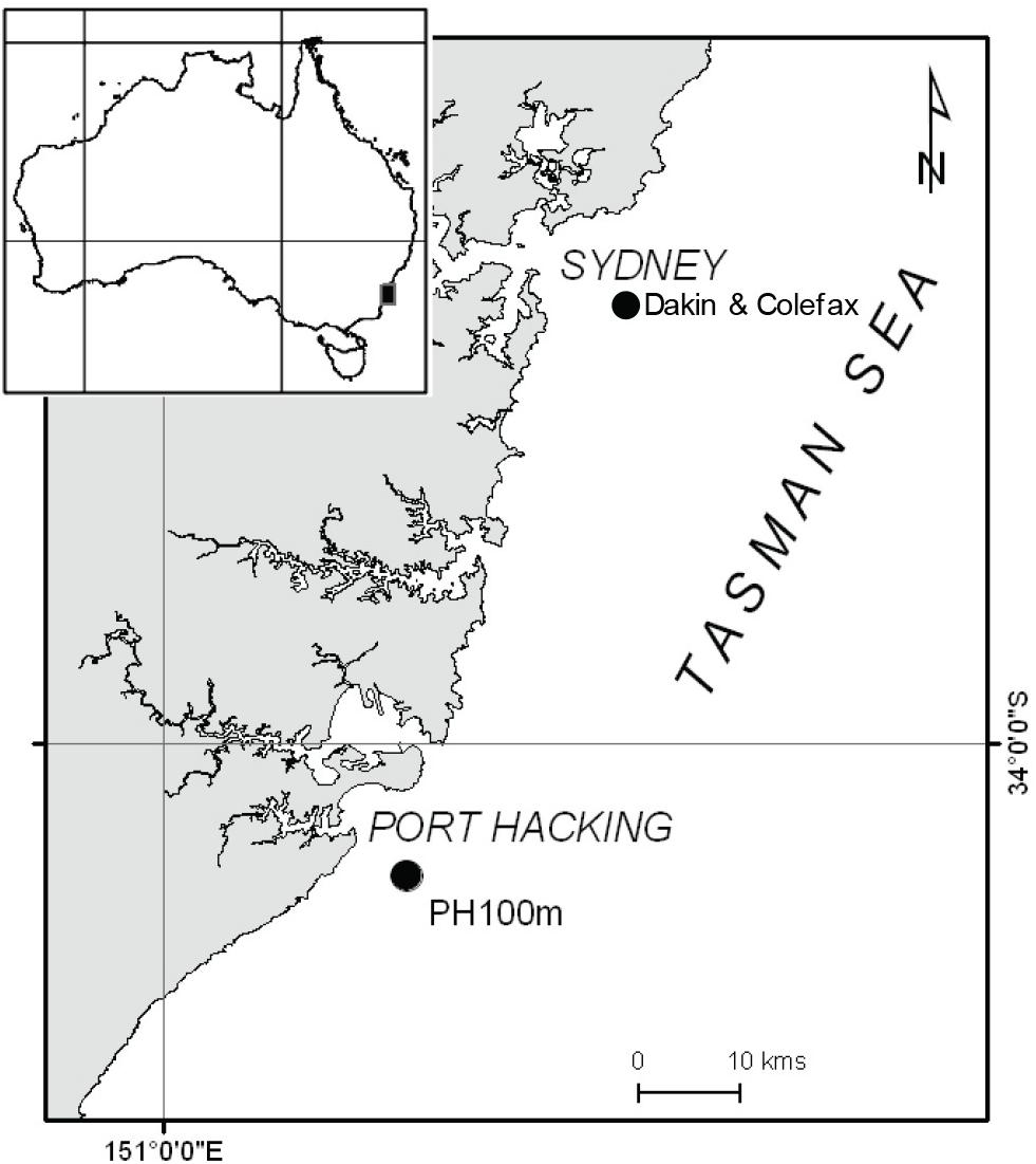
Figure 1. Map of study area showing southeast Australia (inset) and the coastal monitoring stations of Dakin and Colefax (DC) and Port Hacking 100 m (PH_100m) indicated by black circles.

Over the ∼90 years of phytoplankton research at PH_100m, there have been many short-term phytoplankton investigations undertaken (Ajani et al., 2016b) and references therein), but few studies over long time periods. Most recently, using phytoplankton community composition data, the realized niches of phytoplankton were examined over ∼50 years to assess if they were fixed or if they shifted in response to changing environmental conditions at this station (Ajani et al., 2018). Using the Maximum Entropy Modeling framework (MaxEnt) (Phillips and Dudik, 2008), a commonly used algorithm used to model species distributions, it was revealed that the phytoplankton community tracked changes in environmental conditions (temperature, salinity, mixed layer depth, nitrate, and silicate) over decadal time periods at this station. While this study provided the first evidence that biotic communities may be adapting to changing conditions at PH_100m, there has been no examination of the changes in relative composition across this same period in relation to regional warming.

A challenge of analyzing long time series is that often the sampling and analysis methods change over time, making it difficult to attribute change to a particular driver (Brown et al., 2011). For example, estimates of phytoplankton abundance differ depending on whether samples are collected using nets or bottles (Sournia, 1978). However, a careful choice of data analysis method can minimize these biases (Brown et al., 2011). For instance, by comparing changes in relative rather than absolute abundances of species, a more robust assessment of differences in sampling periods attributed to climate impacts can be made (Fodrie et al., 2010; Brown et al., 2011). One such index is the Community Temperature Index (CTI) (Devictor et al., 2008; Stuart-Smith et al., 2015). It is the overall temperature preference of species in a sample, weighted by their abundance, so that more abundant species have greater influence. As it is based on relative rather than absolute composition within a sample, it is less impacted by the variations in sampling methods over time. The CTI has been used extensively to assess the preferred temperature of communities of microbes, butterflies, fish and benthic invertebrates (Devictor et al., 2008; Bates et al., 2013; Cheung et al., 2013; Zografou et al., 2014; Stuart-Smith et al., 2015), although it has never been used for phytoplankton.

Here we use the CTI to investigate changes in relative phytoplankton community composition and temperature spanning 90 years (1931–2020) from PH_100m to examine the response of the phytoplankton community to long-term ocean warming. We answered two key questions: (1) Has the phytoplankton community changed overtime in response to warming; (2) If so, which species are responsible for this change? Insights from these findings are important for identifying sensitive indicators for further monitoring, developing a better understanding of the functional traits of “winners and “losers” under climate change, and the possible flow on effects to other trophic levels dependent on phytoplankton composition and production.

Materials and Methods

From 1965 to 2019, there have been four major phytoplankton sampling surveys at PH_100m (34°7′3.36″S, 151°13′5.52″E, Figure 1). These surveys were carried out during 1965–1966, 1997–1998, 1998–2009, and 2009–2019 and had different sampling frequencies, methods and references (Table 1 and Supplementary Figure S1). A fifth sampling campaign was included in the analyses due to its proximity to PH_100m. This earlier dataset by Dakin and Colefax (1933) was collected ∼6 km east of North Head, Port Jackson, Sydney (max. water depth 55 m; <40 km from PH_100m) from 1930 to 1931. For the remaining analysis, this survey is considered part of the PH_100m dataset (Table 1 and Figure 1).

TABLE 1

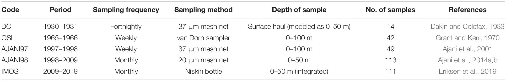
Table 1. Phytoplankton sampling survey codes, frequency, duration, methodology and reference from PH_100m coastal station.

All phytoplankton samples were collected weekly, fortnightly or monthly using either discrete or depth integrated bottle samples (Dorn/Niskin) or phytoplankton mesh nets (20 μm or 37 μm) and preserved before microscopic examination. Cells were identified to the lowest possible taxon using light microscopy and where identification to species level was not possible, cells were assigned to a genus (e.g., Chaetoceros spp., Thalassiosira spp.) according to relevant taxonomic guides (Ajani et al., 2016b).

We used the HadISST1 dataset¹ to assess the temperature change in the area. This is a monthly, 1° gridded product based on in situ and satellite temperature measurements (Rayner et al., 2003). We calculated an annual mean temperature for the 1° grid square around the Port Hacking site.

To investigate whether warming at PH_100m changed the phytoplankton community over the past 90 years, we compared the temperature preference of the phytoplankton community through time (across sampling surveys) using the CTI (Devictor et al., 2008; Stuart-Smith et al., 2015). The CTI is a semi-quantitative index that is reasonably robust to different sampling devices. It is calculated as a community-weighted mean of the thermal preference of a community based on the individual temperature preferences of each species [species temperature index (STI)], and as such is reasonably robust to different water volumes captured. It is calculated as a community weighted mean of the thermal preference of a community based on the individual temperature preferences of each species (STI). It is normally calculated on a per sample basis. We calculated the CTI based on species that have been found across multiple surveys because this indicates species that are more likely to be consistently identified by different taxonomists, and it is less biased by species only identified in one particular survey. Thus, an increase in the CTI indicates that the proportion of species with warmer preferences have increased and/or there has been a decrease in the proportion of species with cooler temperature preference.

For the CTI analysis, the first stage was to calculate the STI for the species in the sampling surveys at PH_100m. To do this we combined 329 phytoplankton samples collected across five sampling surveys from 1930 to 2019 and from these samples, we selected the species that had been consistently identified across the sampling periods, rejecting those that were not verifiable based on published taxonomic information. From this group of species, we then selected those that had been identified in the IMOS sampling period and at least one other survey at PH_100m. From these, 30 species were retained as consistently identified and were included in the analysis of CTI (Supplementary Tables S1, S2).

The STIs were calculated using Australia’s Integrated Marine Observing Systems (IMOS) long-term plankton datasets from the National Reference Stations (∼750 samples) (Eriksen et al., 2019) and the Australian Continuous Plankton recorder survey (∼6000 samples) (Davies et al., 2016), The National Reference Station and Continuous Plankton Recorder surveys have analyzed phytoplankton in a consistent manner for 12 years and provide abundance data for phytoplankton across the full temperature range of Australian waters and beyond. The sea surface temperature for each sample over the past 12 years was sourced from the GHRSST L4 gridded product, which gives daily temperature over a 10 km resolution based on the time, latitude and longitude of the sample². We extracted every abundance record for the 30 retained species from this dataset and fitted these, with the associated temperature for each sample, to a Kernel Density Estimation (KDE) function. This is a non-parametric smoothing technique used to estimate the probability density function of a random variable. The temperature at the maximum point of the Kernel Density curve, the temperature of maximum abundance, is defined as the STI for each species.

Using the STI information for each species (s), the CTI was then calculated as the mean temperature preference of the species in a sample (Devictor et al., 2008):

$$\mathrm{Community}\mathrm{Temperature}\mathrm{Index}\left(\mathrm{CTI}{}^{\circ }\mathrm{C}\right)={\displaystyle \sum _{\mathrm{s}=1}^n}={\text{STI}}^{\circ }\mathrm{C}\left(\mathrm{s}\right)\times \mathrm{Relative}\mathrm{Abundance}(s)$$

To understand if CTI had changed over time we used a linear model with the CTI as the response and Period and Month as predictors (Supplementary Table S3). Period was modeled as a factor including a level for each survey. We adjusted for the seasonal cycle by including Month as a factor in the model. This compensates for the bias introduced by the frequency and timing of the samples. If more samples in a particular sampling period were collected in the warmer months we would expect the CTI to be higher than if more samples were collected in the colder months. Accounting for the month compensates for this variation so the model is testing the long term response of CTI.

Although CTI is robust to differences between sampling methods we also tested for effects of the variation in sampling design over time. We added predictors for Method (with two levels: bottle, net) and Depth (with two levels: 0–50 m, 0–100 m) (see Table 1) to the linear model, but neither predictor turned out to be significant (p > 0.05) supporting the assumptions we have made in using this analysis technique. Both predictors were dropped from the final model.

The CTI represents the overall temperature preference of the community present, and has units of °C. Because the CTI is defined on temperature, we expect it to be sensitive to changes in temperature (warming) and not other environmental variables. However, we investigated the importance of other available environmental variables (i.e., nitrate and phosphate; silicate was not included because it was only available for the most recent two sampling periods) in our linear models and found they were unrelated to CTI (Supplementary Table S3). Note that our CTI analysis and the focus on temperature contrasts with an analysis of the general drivers of phytoplankton communities using multivariate analyses of raw species abundances and including multiple potential environmental drivers. Unfortunately, such an analysis was not possible here because the phytoplankton data over the 90 years was sampled with different methods and so the CTI, with its ability to use relative abundance data, was considered more appropriate.

All the analyses were performed in R³, using tidyverse, ggplot2, and visreg packages. The KDE for calculating STI was performed using the density() function in the stats package.

Finally, as a decline in cooler-water species and an increase in warmer-water species can both contribute to an increase in the CTI, we then investigated the species primarily responsible for the increase in CTI over time. We selected the five most abundant species from each survey used in the CTI calculation. As the dominant species were mostly consistent across surveys, this resulted in a total of eight species, which we investigated further.

Caveats

There are several caveats of combining disparate datasets over time such as we have done in the present study. Firstly, the data in the present study focuses on the most frequently observed, taxonomically verified species, i.e., the diatoms. Dinoflagellates are often poorly resolved using preservatives such as Lugol’s Iodine and light microscopy. On the other hand, however, the phytoplankton taxa used to calculate the thermal preferences in our current study (predominantly the diatoms) might be a true reflection of a diatom-dominated community at this location (Ajani, 2014; Ajani et al., 2014b). We have also carefully curated the species lists included in these analyses to include only species that an experienced analyst could reliably and repeatedly identify over the various surveys. We assessed taxa stability (defining characteristics, the ease of discrimination with light microscopy, any drawings, diagrams, photographs or taxonomic descriptions that would have been available to all analysts) over the entire period and made expert consensus decisions on which taxa to retain. We traced nomenclatural changes through the World Register of Marine Species (WoRMS) and thus could reconstruct the community composition recorded in the past with contemporary nomenclature. This is important as it not possible to re-examine the material from previous surveys, and indeed that may introduce a further bias in the results. We discarded observations only made to genus or higher levels as they do not add to or improve the analysis.

Results

Species temperature index across all taxa ranged from 16.65°C (Noctiluca scintillans) to 24.73°C (Tripos candelabrum) with an average of 20.3°C. Kernel density plots of these eight dominant species (seven diatoms and one dinoflagellate) show the range of their thermal preferences (Figure 2). The STI for the most abundant species ranged from 17 to 23°C, clustered around 20.8°C, similar to the mean water temperature over the IMOS sampling period (21°C, Figure 3). Species with narrower, taller peaks are more stenothermal (e.g., Asterionellopsis glacialis), whilst species with broader curves are more eurythermal (e.g., Proboscia alata).

FIGURE 2

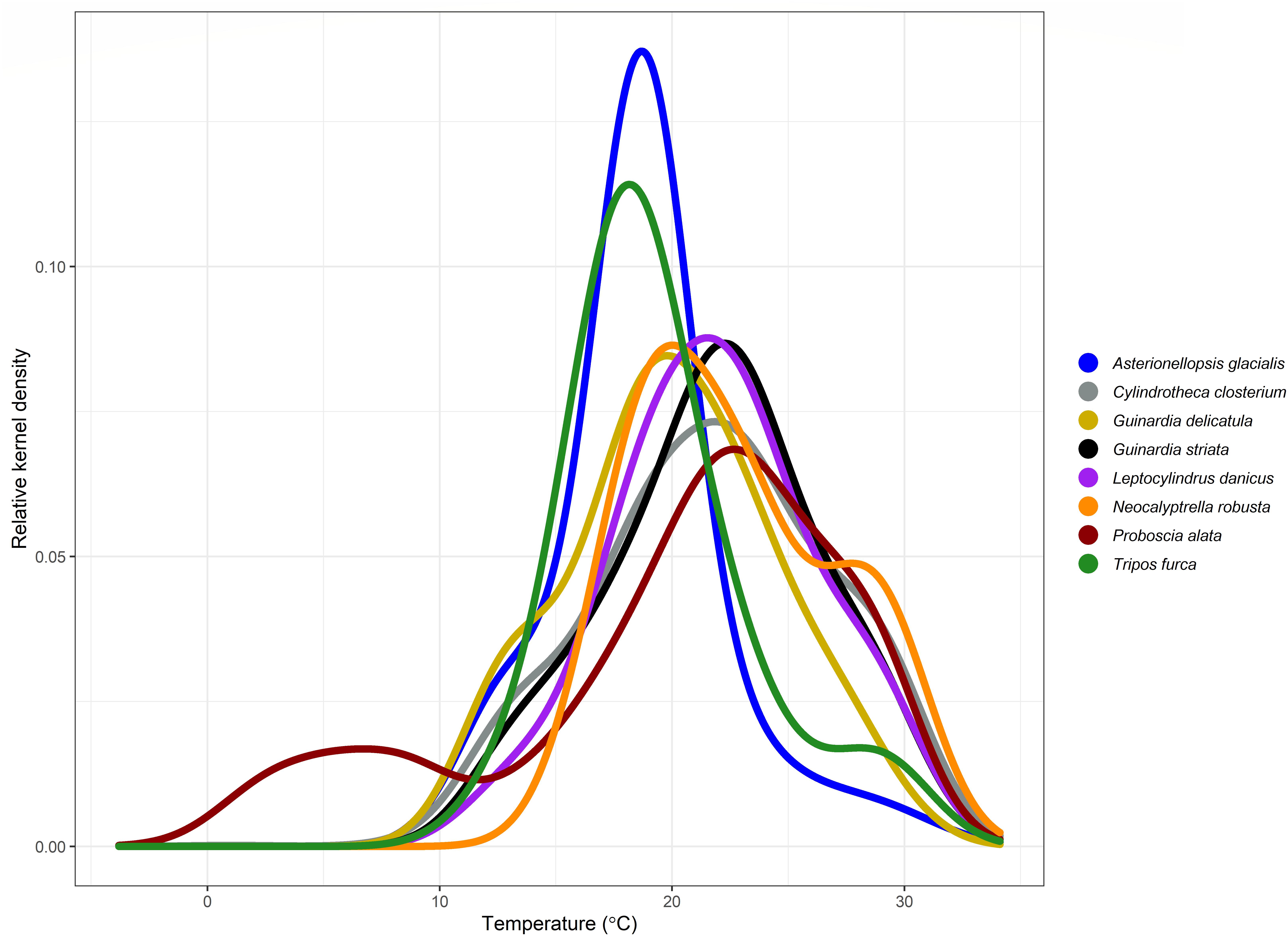
Figure 2. Kernel density plots showing the temperature preferences (STIs) of the top eight most abundant species for each survey at PH_100m.

FIGURE 3

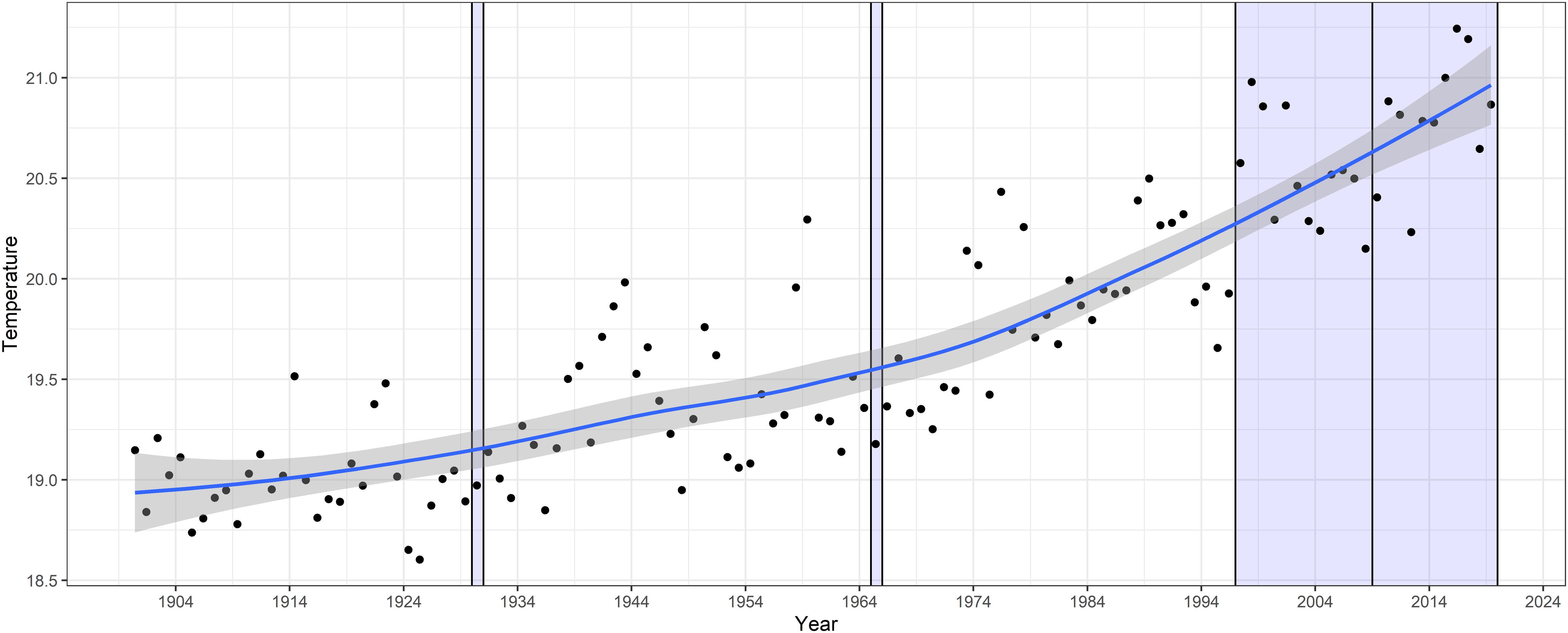
Figure 3. Annual mean and 95% confidence levels of long-term temperature at PH_100m from Hadley SST with phytoplankton surveys marked by lines and shaded regions.

The model output indicates an increase in CTI over time, with the significance values of each period relative to the 1930s increasing with time (1965–1966, p = 0.4; 1997–2009, p = 0.03; 2009–2019, p = 0.0001) (Figure 4A). The mean CTI of samples increased from 20.4°C in 1931–1932 to 21.2°C from 2009 to 2019. The wider range of CTI shown in the 1997–2009 and 2009–2019 sampling periods is due to the much larger number of samples and thus the wider range of environmental conditions sampled. The increase in CTI of 0.8°C across all years, was consistent in direction with warming over the same period at PH_100m (Figure 3). However, the warming of 1.8°C was substantially greater than the increase in CTI of 0.8°C for the same period. A clear seasonal cycle in CTI was also observed, with highest values toward the end of the austral summer (February/March) and lowest at the end of winter (August/September) (Figure 4B). The seasonal variation in CTI agrees with the trend of water temperatures across seasons at PH₁₀₀, although it is not as pronounced, and reflects the changing thermal preference of the community across season.

FIGURE 4

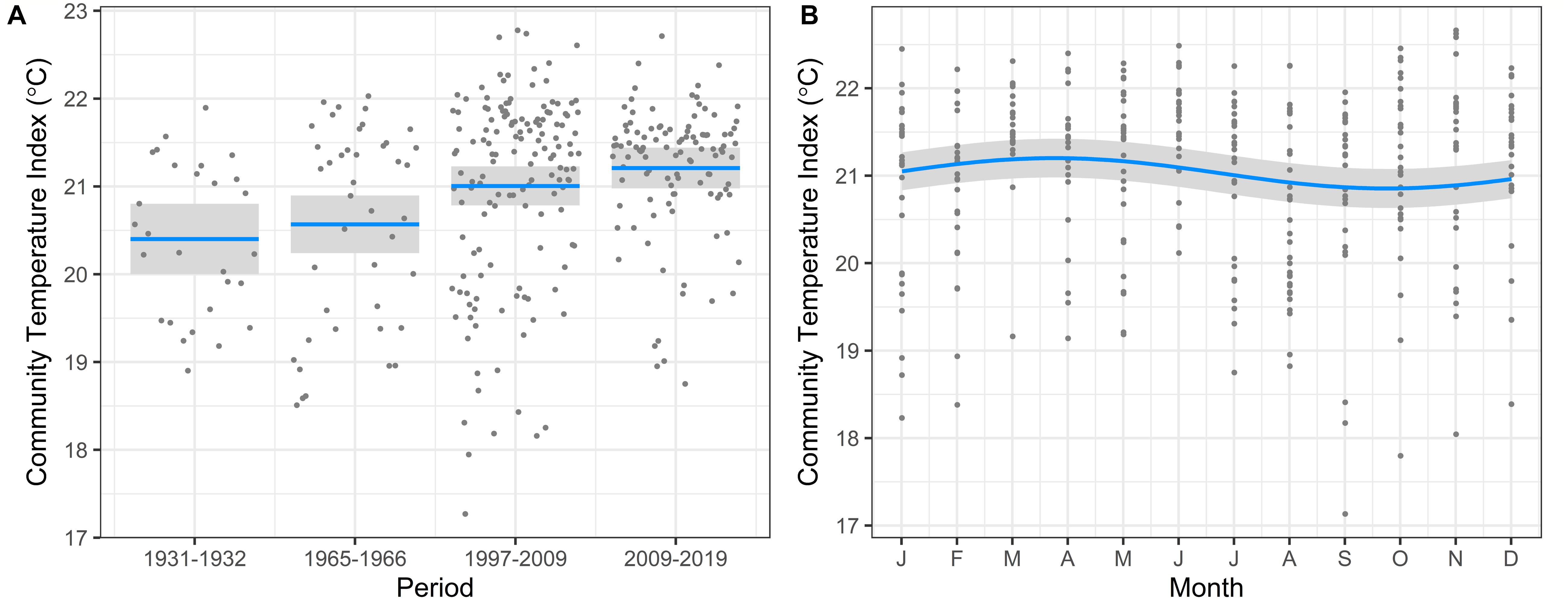
Figure 4. Model output showing variation in Community Temperature Index in response to (A) Time period, and (B) Month, over 90 years of phytoplankton abundance data from PH_100m. Mean CTI shown by blue line and 95% confidence intervals by shaded areas.

There were substantial changes in the relative proportion of several of the eight dominant species for each time period (Figure 5). The generally cooler water, chain-forming diatom A. glacialis (STI = 18.7°C) substantially decreased in abundance overtime (40% in 1931–1932 to 13% in 2009 onward). There were also declines over time in the dinoflagellate Tripos furca (STI = 18.2°C, 9–1.6%), and the diatom Guinardia striata (STI = 22.3°C, 7.3–2.3%), while the diatom Neocalyptrella robusta (STI = 20.0°C) was observed in the 1930s (12%) but infrequently since (close to 0%). By contrast, the warmer-water diatom species Leptocylindrus danicus (STI = 21.5°C; 20% in 1931–1932 to 57% in 2009 onward), Cylindrotheca closterium (STI = 21.9°C, 0–7%) and P. alata (STI = 22.7°C, 1.8–8.2%) all substantially increased in abundance over time. The cool-affinity diatom Guinardia delicatula (STI = 19.8°C, 1–7%) also increased in abundance overtime.

FIGURE 5

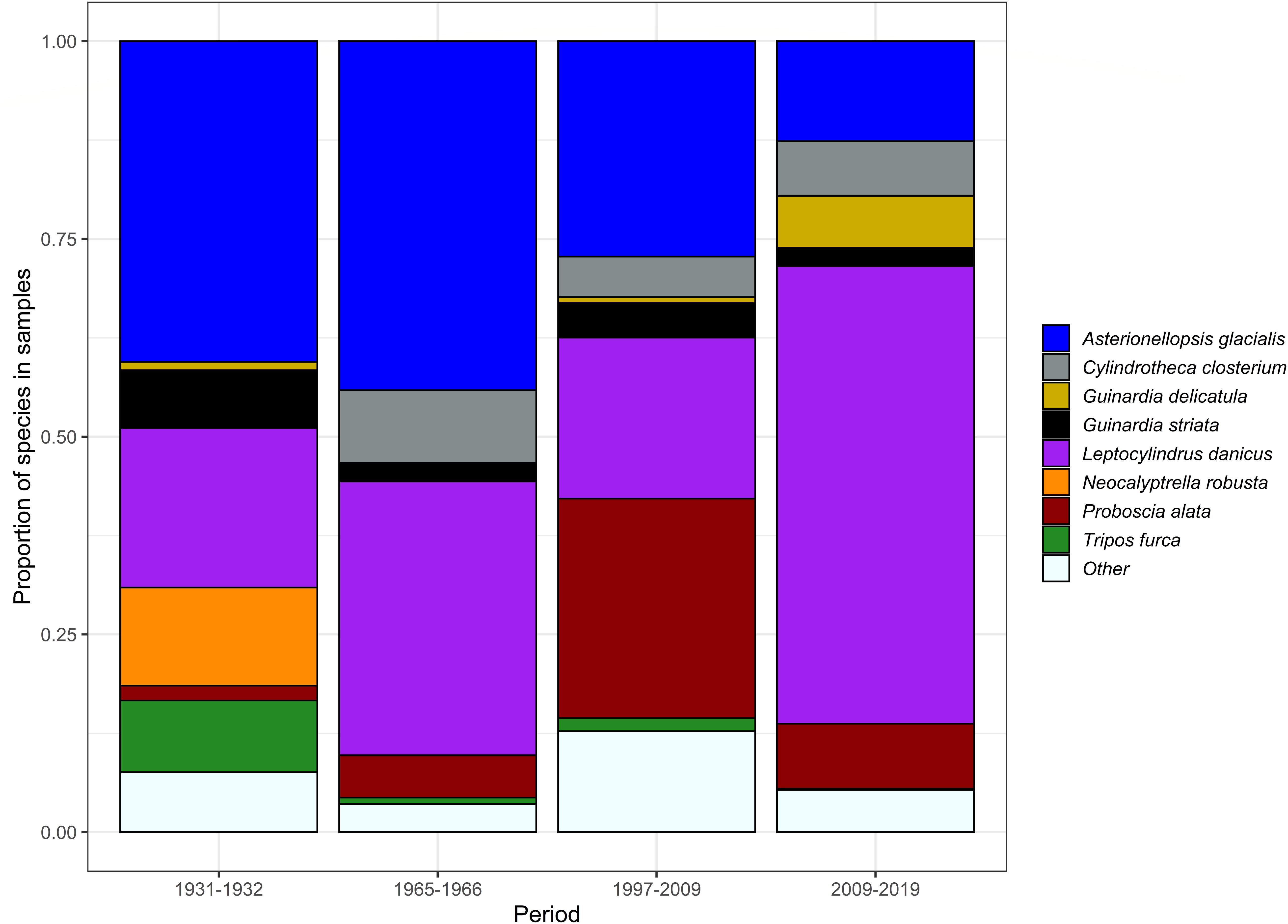
Figure 5. Relative proportion of the dominant phytoplankton species from each sampling survey at PH_100m and their relative shifts in abundance from 1930 to 2019.

Discussion

Increase in Community Temperature Index at Port Hacking

Despite the dynamic nature of PH_100m, with a phytoplankton community that exhibits orders of magnitude variation over daily, weekly, seasonal and inter-annual time scales, there is still a clear increase in CTI at this location. The most pronounced of this “short term” variability is a result of wind-driven or current-driven upwelling which brings cold, nutrient-rich (phosphate, silicate, and nitrate) water into the euphotic zone and causes diatom blooms (Ajani et al., 2001). These slope water intrusions can last between 2 and 22 days, most commonly from September to February (Lee et al., 2001, 2007; Pritchard et al., 2003). Seasonal variation is also well-defined at PH_100m, with the water column well mixed between May and September (decreasing in recent years) and highly stratified from December to March (Grant and Kerr, 1970; Ajani et al., 2001). Notwithstanding these well-documented patterns in the phytoplankton community at this location, these studies are still considered “short term” in relation to climate change. Using disparate datasets over much longer sampling periods (including the present study), emerging evidence suggests that the phytoplankton community at this location may track the magnitude and direction of environmental change also occurring in this region (Ajani et al., 2018). Indeed, the overall shift to a warmer community at PH_100m is most likely a consequence of the strengthening of the East Australian Current along this coastline. The increasing southerly flow of the EAC, and significant warming documented in this region, have not only seen the poleward shift in certain phytoplankton species (Ajani et al., 2014a,b; Buchanan et al., 2014) and larger species such as invertebrates and fish (Ling et al., 2009; Figueira and Booth, 2010; Last et al., 2011), but is predicted to cause a substantial shift in the microbial assemblage structure and function along this coastline (Messer et al., 2020).

Smaller Increase in Community Temperature Index Than Warming

Interestingly, the shift we observed in the CTI (0.8°C) is less than that observed in the regional temperature data (1.8°C). This may be for a number of reasons. While the increase in CTI at PH_100m may be due to an increase in the abundance of warm-water species such as L. danicus and a decrease in cold-water species such as A. glacialis, it may also be affected (reduced) by a decrease in other warm-water species (e.g., G. striata) or an increase in cold-water species (e.g., G. delicatula). These latter two species however, were far less abundant than L. danicus or A. glacialis at PH_100m, and although contributing to the overall CTI, would have had significantly less impact than the more abundant species.

Furthermore, it may be a consequence of the shorter time scales in variation of SST data compared to a lagged response by the phytoplankton community. The phytoplankton data examined does not include the whole phytoplankton community, but rather a subset of consistently and unequivocally identified taxa. STIs cannot be calculated for rare species due to the need for a minimum number of observations for a statistically robust result. As our final data set only includes relatively abundant, larger species that can be identified using microscopy and that we were confident were consistently and correctly identified across surveys (∼20% of the phytoplankton community), our results should be interpreted with caution; changes in rarer, smaller (picoeukaryotes) or species with narrow temperature preferences may also significantly impact the marine food web under climate change.

Species diversity may also confound this signal with changes in individual species having less effect on the CTI at PH_100m due to it relatively high diverse community composition. Moreover, our study has only considered temperature, and to a lesser degree nitrate and phosphate (found to be unrelated to CTI), yet it is the combination and interaction of all physico-chemical parameters (including nutrients, light and CO₂) that will influence marine community structure. The Port Hacking coastal location has seen an increase in temperature, salinity, and nitrate and a decline in silicate recorded at this station over the past 60 years (Thompson et al., 2009). However, not all responses to physico-chemical variables are the same, and although out of the scope of the present study, larger scale oceanic processes or extreme event such as heat waves, must also been taken into account (Trainer et al., 2020). Finally, microbial assemblages are highly diverse and complex, often with thousands of species networking and interacting on both short (e.g., predation) and long-term time scales (e.g., competition), and with an enormous range of behaviors (sinking, buoyancy and vertical migration), life forms (single cell, colonies, spines etc.) and reproductive strategies (sexual, asexual, cyst formation etc.) (Barton et al., 2016). Therefore, although the CTI is a valuable community level metric to evaluate how well communities are suited to their thermal environments (Flanagan et al., 2019), other eco-physiological traits and bioprocesses, life history strategies and phytoplankton assemblage characteristics need to be considered when discussing the response of marine communities to temperature changes.

Potential Winners and Losers Under Climate Change

The species that contributed most to the increase in CTI at PH_100m was the warm-water species L. danicus. This diatom is a major component of coastal upwelling communities’ worldwide (Nanjappa et al., 2013; Karthik et al., 2017) and a dominant member of the phytoplankton community along the south east coast of Australia (Ajani, 2014; Ajani et al., 2014b, 2016a). L. danicus reproduces rapidly (both sexually and asexually) and forms highly silicified resting spores under nutrient depletion. In a recent study to quantify the trait variability within and among closely related Leptocylindrus species, thirty-five isolates were established from six locations spanning 2000 km of the south-eastern Australian coastline (Ajani et al. under review). Comparable to levels of genetic diversity found across similar seascapes, significant intraspecific trait variability was observed for 8 of 9 traits measured (growth rate, biovolume, C:N, silica deposition, silica incorporation rate, chl-a, and photosynthetic efficiency under dark adapted, growth irradiance, and high light adaptation), providing evidence that L. danicus may rapidly adapt to fluctuating conditions. As such, it is this rapid reproduction, resting spore formation, and extremely high morphological and physiological strain variability that could be the functional traits necessary to be a “winner” under climate change.

Conversely, the cool-affinity, chain-forming diatom A. glacialis, which had a narrower thermal range compared with many other species from PH_100m, substantially declined in abundance overtime at PH_100m. This species has been reported to form highly dense (9.32 × 10⁷ cells L^–1), monospecific blooms as a result of upwelling events (cool, nutrient rich waters into the euphotic zone), most notably in India (Mishra and Panigrahy, 1995; Sahu et al., 2016), and along the east coast of Australia from Ballina Beach to Coffs Harbor (200 km) (Ajani et al., 2011). The first records of Asterionellopsis glacialis (as Asterionella glacialis) were by Castracane (1886) who examined Antarctic samples from the HMS Challenger voyages and as the name suggests, this mostly neritic species is more abundant in cold to temperate coastal waters (Hasle and Syvertsen, 1997). It is an “ecologically important planktoner” (Kaczmarska et al., 2014) because of its inclusion in the top 21 species (including L. danicus) that contribute ∼90% of the global biomass produced by diatoms (Leblanc et al., 2012). Under ideal conditions, it blooms repeatedly over one growing season, often in nuisance proportions, and is tolerant of a wide range of temperature, irradiance, energy (estuaries, open ocean and surf-zones) and salinity conditions (Smayda, 1958; Abreu et al., 2003; Kaczmarska et al., 2014). Wood (1964a) noted both species as important at Port Hacking and specifically noted Asterionellopsis (described using the invalid name Asterionellopsis japonica throughout his works, following Cleve (Crosby and Wood, 1959) as an expected component of winter blooms in June and July. In contrast to L. danicus though, the narrower thermal range of A. glacialis combined with the sustained increase in surface water temperature over the study period at PH_100m, allows us to speculate that this taxa may further decline at this site under climate change.

Other diatom species in the “top eight” that increased in abundance over the study period were C. closterium, G. delicatula, and P. alata. The centric diatom G. delicatula (STI = 19.8°C) was rarely observed in the early monitoring campaigns (DC, OSL, and Ajani), but is now one of the most frequently observed species in the IMOS monitoring (Supplementary Table S1). This species is known to form non-toxic high biomass blooms worldwide but was not noted as present at Port Hacking (Wood, 1964a) in his extensive surveys. Control of bloom dynamics of G. delicatula in the northern hemisphere is linked to infection by phagotrophic nanoflagellates (Drebes et al., 1996) and viruses (Arsenieff et al., 2019), but to date this has not been established for populations at Port Hacking. Increased frequency of occurrence may be linked to apparent ability to grow at lower Si:C ratios than other diatoms (Rousseau et al., 2002), however, incomplete nutrient records in our early monitoring campaigns mean that long-term changes in nutrient ratios cannot be easily tested. Rousseau et al. (2002) also noted increasingly earlier bloom timings linked to higher than average water temperatures in the North Sea, and the survival of larger overwintering populations and this may also explain the increase in abundance over time at Port Hacking.

The cosmopolitan benthic marine diatom C. closterium (STI = 21.9°C) was noted as quantitatively unimportant in coastal NSW by Dakin and Colefax (1933), but the “most commonest diatom in the estuarine environment” by Crosby and Wood (1959). Its broad distribution globally and ecological success is likely enhanced by its ability to disperse easily from sediments into the water column, high genetic diversity and genotypes with a range of thermal niches (Stock et al., 2019). In their global comparison of strains of C. closterium, Stock et al. (2019) reported a clonal culture isolated from Port Hacking showed optimal growth above 20°C, with wide variability in strain specific maximum growth rates.

P. alata (STI = 22.7°C) is a common oceanic species with wide distribution globally (Dakin and Colefax, 1933), with one varietal form (var. indica) described as extremely stenothermal (Schöne, 1982), however, this observation is not supported by the broad temperature preference exhibited by this species at Port Hacking (Figure 2). Noted as one of the top 20 taxa in the OSL study (Grant and Kerr, 1970), P. alata was one of 15 common phytoplankton taxa identified to have shifted southward in its distribution along the east coast of Australia (Richardson et al., 2015) relative to its mean position prior to 1990. Much of the published data on growth rates and ecological niches for this species focus on polar regions, partly because of the occurrence of distinct winter and spring forms (Jordan et al., 1991), and the species prevalence in large diatom-dominated spring blooms. There is comparatively little information on its autecology and favored niches in temperate communities.

Species in the “top eight” that decreased in abundance over the study period included G. striata, N. robusta, and T. furca. G. striata (STI = 22.3°C) is rarely mentioned in early studies from Port Hacking, but is another species noted for its low silica requirements and ability to form blooms in silica-deplete conditions (Schapira et al., 2008). G. striata was one of 87 North Atlantic phytoplankton taxa modeled (as Rhizosolenia stolterfothii) for future changes in geographic distribution based on historical CPR data (1951–2000) and future ocean conditions (2051–2100) (Barton et al., 2016). Consistent longitudinal shifts reflected dynamical changes in multiple environmental drivers (temperature, nutrients, stratification/mixed layer depth, etc.) on top of expected latitudinal range shifts commonly attributed to temperature alone.

The only dinoflagellate present in the “top eight” was T. furca (STI = 18.2°C) noted to be tolerant of a wide range of temperatures and observed in estuarine, neritic and oceanic waters, but absent from polar and sub-polar seas (Dakin and Colefax, 1933). This species can be up to 50% of the dinoflagellate community in nearshore/estuarine environments (Wood, 1964a), often present year-round but in notably lower concentrations in winter (Dakin and Colefax, 1933). T. furca decreased in abundance from 9 to 1.6% over the study period suggesting a preference for lower temperatures, consistent with its inclusion in the 15 species showing a southward movement off the East coast of Australia (Richardson et al., 2015). Finally, N. robusta (STI = 20.0°C) was present in the earliest dataset (DC), but not detected in OSL, Ajani or Ajani2 datasets. The species was described as a “warm oligo-eurytherm” diatom and proposed as an indicator of warm water currents from tropical or subtropical areas (Baars, 1982). It has not been observed in “cold” waters (Hernandez-Becerril and Del Castillo, 1996).

Conclusion

Based on one of the longest time series of phytoplankton in the Southern Hemisphere (90 years), and using a community-level temperature index, we found a significant warming signature in the phytoplankton community overtime. The phytoplankton CTI also showed strong seasonality, with highest values observed toward the end of the austral summer (February/March) and lowest at the end of winter (August/September), a well-recognized temporal pattern for this location. Species whose abundance changed substantially over time, and resulted in the observed increase in the CTI, were Leptocylindrus danicus and Asterionellopsis glacialis among others, providing insights into the potential functional traits–broad/narrow thermal range, formation of resting spores, and high phenotypic/genotypic variability–that may determine the adaptive capacity or survivability of species under climate change.

Data Availability Statement

Publicly available datasets were analyzed in this study. This data can be found here: https://portal.aodn.org.au/.

Author Contributions

PA, CD, and AR were responsible for the conceptualization of this work. CD performed the analysis. All authors were responsible for the writing, reviewing, and editing of this manuscript.

Conflict of Interest

The authors declare that the research was conducted in the absence of any commercial or financial relationships that could be construed as a potential conflict of interest.

Acknowledgments

We acknowledge all contributors, past and present to the PH_100m time-series dataset especially Prof. Gustaaf Hallegraeff, Ms. Alex Coughlan, Dr. Tim Ingleton, and Dr. Andrew Allen. National Reference Station data are sourced from the Integrated Marine Observing System (IMOS). IMOS is a national collaborative research infrastructure, supported by the Australian Government. All data are available through the Australian Ocean Data Network (AODN) portal (https://portal.aodn.org.au/search). The data used for calculating the STIs can be sourced from the AusCPR and NRS data collections and the other datasets are included in the Australian Phytoplankton Database (Davies et al., 2016). The data collection titles at the AODN are as follows: IMOS–AusCPR: Phytoplankton Abundance; IMOS National Reference Station (NRS)–Phytoplankton Abundance and Biovolume; The Australian Phytoplankton Database (1844–ongoing)–Abundance and Biovolume.

Supplementary Material

The Supplementary Material for this article can be found online at: https://www.frontiersin.org/articles/10.3389/fmars.2020.576011/full#supplementary-material

Supplementary Figure 1 | Sampling frequency across each sampling survey from 1930 to 2019 at PH_100m, southeastern Australia.

Supplementary Table 1 | A list of the taxa, their Species Temperature Index (STI), and the number of times each was reported in a sample from the PH_100m coastal station from each sampling campaign, 1930–2019. LowerSST and UpperSST represent lower and upper quartile temperatures from Kernel Density Plots for each species. Note NA = no report for this species in this sampling period. Species with ^∗ indicate those that were the top eight most abundant across all surveys and included in Figure 5.

Supplementary Table 2 | (A) Species not used as consistent identification could not be verified across surveys. (B) Species not used as didn’t occur in the IMOS survey plus one other survey. (C) Species not used as not enough data to calculate a STI, i.e., rare species not seen more than 30 times over the IMOS NRS and AusCPR surveys across Australia.

Supplementary Table 3 | Linear model outputs. Note: In the second model neither the NOX nor the seasonal cycle are significant, but we see an increase in relative significance between the periods. The nitrate data was from the long-term monitoring survey at Port Hacking but was not associated directly with the samples, therefore a climatology was used to estimate the nitrate at each sample time confounding the effect of season across the model. The first model includes a wider time range, maintains a good level of significance between periods and has a weakly significant seasonal cycle. This is the more robust model.

Footnotes

1. ^ https://www.metoffice.gov.uk/hadobs/hadisst/data/download.html
2. ^ https://www.ghrsst.org/ghrsst-data-services/services/
3. ^ https://www.r-project.org/

References

Abreu, P. C., Rorig, L. R., Garcia, V., Odebrecht, C., and Biddanda, B. (2003). Decoupling between bacteria and the surf-zone diatom Asterionellopsis glacialis at Cassino Beach, Brazil. Aquat. Microb. Ecol. 32, 219–228. doi: 10.3354/ame032219

CrossRef Full Text | Google Scholar

Ajani, P. A. (2014). Phytoplankton Diversity in The Coastal Waters of New South Wales, Australia. Macquarie Park, NSW: Macquarie University.

Google Scholar

Ajani, P. A., Allen, A. P., Ingleton, T., and Armand, L. (2014a). A decadal decline in relative abundance and a shift in microphytoplankton composition at a long-term coastal station off southeast Australia. Limnol. Oceanogr. 59, 519–531. doi: 10.4319/lo.2014.59.2.0519

CrossRef Full Text | Google Scholar

Ajani, P. A., Allen, A. P., Ingleton, T., and Armand, L. (2014b). Erratum: A decadal decline in relative abundance and a shift in phytoplankton composition at a long-term coastal station off southeast Australia. Limnol. Oceanogr. 59, 2240–2242. doi: 10.4319/lo.2014.59.6.2240

CrossRef Full Text | Google Scholar

Ajani, P. A., Armbrecht, L. H., Kersten, O., Kohli, G. S., and Murray, S. A. (2016a). Diversity, temporal distribution and physiology of the centric diatom Leptocylindrus Cleve (Bacillariophyta) from a Southern Hemisphere upwelling system. Diatom Res. 31, 351–365. doi: 10.1080/0269249x.2016.1260058

CrossRef Full Text | Google Scholar

Ajani, P. A., Hallegraeff, G., Allen, D., Coughlan, A., Richardson, A. J., Armand, L., et al. (2016b). Establishing baselines: a review of eighty years of phytoplankton diversity and biomass in southeastern Australia. Oceanogr. Mar. Biol. Annu. Rev. 54, 387–412.

Google Scholar

Ajani, P., Ingleton, T., Pritchard, T., and Armand, L. (2011). Microalgal blooms in the coastal waters of New South Wales, Australia. Proc. Linn. Soc. New South Wales 133:15.

Google Scholar

Ajani, P., Lee, R., Pritchard, T., and Krogh, M. (2001). Phytoplankton dynamics at a long-term coastal station off Sydney, Australia. J. Coast. Res. 34, 60–73.

Google Scholar

Ajani, P. A., McGinty, N., Finkel, Z. V., and Irwin, A. J. (2018). Phytoplankton realized niches track changing oceanic conditions at a long-term coastal station off Sydney Australia. Front. Mar. Sci 5:285. doi: 10.3389/fmars.2018.00285

CrossRef Full Text | Google Scholar

Arsenieff, L., Simon, N., Rigaut-Jalabert, F., Le Gall, F., Chaffron, S., Corre, E., et al. (2019). First viruses infecting the marine diatom Guinardia delicatula. Front. Microbiol. 9:3235. doi: 10.3389/fmicb.2018.03235

PubMed Abstract | CrossRef Full Text | Google Scholar

Baars, J. W. M. (1982). Autecological investigation on marine diatoms - Thalassiosira nordenskioeldii and Chaetoceros diadema. Mar. Biol. 68, 343–350. doi: 10.1007/bf00409599

CrossRef Full Text | Google Scholar

Barrera-Alba, J. J., Abreu, P. C., and Tenenbaum, D. R. (2019). Seasonal and inter-annual variability in phytoplankton over a 22-year period in a tropical coastal region in the southwestern Atlantic Ocean. Cont. Shelf Res. 176, 51–63. doi: 10.1016/j.csr.2019.02.011

CrossRef Full Text | Google Scholar

Barton, A. D., Irwin, A. J., Finkel, Z. V., and Stock, C. A. (2016). Anthropogenic climate change drives shift and shuffle in North Atlantic phytoplankton communities. Proc. Natl. Acad. Sci. U.S.A. 113, 2964–2969. doi: 10.1073/pnas.1519080113

PubMed Abstract | CrossRef Full Text | Google Scholar

Bates, A. E., McKelvie, C. M., Sorte, C. J. B., Morley, S. A., Jones, N. A. R., Mondon, J. A., et al. (2013). Geographical range, heat tolerance and invasion success in aquatic species. Proc. Royal Soc. B Biol. Sci. 280:1772.

Google Scholar

Benway, H. M., Lorenzoni, L., White, A. E., Fiedler, B., Levine, N. M., Nicholson, D. P., et al. (2019). Ocean time series observations of changing marine ecosystems: An era of integration, synthesis, and societal applications. Front. Mar. Sci 6:393. doi: 10.3389/fmars.2019.00393

CrossRef Full Text | Google Scholar

Brown, C. J., Schoeman, D. S., Sydeman, W. J., Brander, K., Buckley, L. B., Burrows, M., et al. (2011). Quantitative approaches in climate change ecology. Glob. Change Biol. 17, 3697–3713.

Google Scholar

Buchanan, P. J., Swadling, K. M., Eriksen, R. S., and Wild-Allen, K. (2014). New evidence links changing shelf phytoplankton communities to boundary currents in southeast Tasmania. Rev. Fish Biol. Fish. 24, 427–442. doi: 10.1007/s11160-013-9312-z

CrossRef Full Text | Google Scholar

Castracane, F. (1886). Report on the Diatomaceae Collected by H. M. S. Challenger During the Years 1873–1876. Report on the Scientific Results of the Voyage of H. M. S. Challenger During the Years 1873–76. Botany. 2 (Part 4): 1–178, pl. 1–30. Available online at: http://www.19thcenturyscience.org/HMSC/HMSC-Reports/Bot-04/README.htm

Google Scholar

Cheung, W. W. L., Pauly, D., and Sarmiento, J. L. (2013). How to make progress in projecting climate change impacts. ICES J. Mar. Sci. 70, 1069–1074. doi: 10.1093/icesjms/fst133

CrossRef Full Text | Google Scholar

Crosby, L. H., and Wood, E. J. F. (1959). Studies on australian and new zealand diatoms II.—normally epontic and benthic genera. Trans. Royal Soc. New Zeal. 86, 1–58.

Google Scholar

Dakin, W. J., and Colefax, A. N. (1933). The marine plankton of the coastal waters of New South Wales. I, The chief planktonic forms and their seasonal distribution. Proc. Linn. Soc. New South Wales 58, 186–222.

Google Scholar

Davies, C. H., Coughlan, A., Hallegraeff, G., Ajani, P., Armbrecht, L., Atkins, N., et al. (2016). A database of marine phytoplankton abundance, biomass and species composition in Australian waters. Sci. Data 3:160043.

Google Scholar

Deppeler, S. L., and Davidson, A. T. (2017). Southern ocean phytoplankton in a changing climate. Front. Mar. Sci 4:40. doi: 10.3389/fmars.2017.00040

CrossRef Full Text | Google Scholar

Devictor, V., Julliard, R., Couvet, D., and Jiguet, F. (2008). Birds are tracking climate warming, but not fast enough. Proc. Royal Soc. B Biol. Sci. 275, 2743–2748. doi: 10.1098/rspb.2008.0878

PubMed Abstract | CrossRef Full Text | Google Scholar

Doney, S. C. (2006). Oceanography - Plankton in a warmer world. Nature 444, 695–696. doi: 10.1038/444695a

PubMed Abstract | CrossRef Full Text | Google Scholar

Doney, S. C., Lindsay, K., Fung, I., and John, J. (2006). Natural variability in a stable, 1000-yr global coupled climate-carbon cycle simulation. J. Clim. 19, 3033–3054. doi: 10.1175/jcli3783.1

CrossRef Full Text | Google Scholar

Doney, S. C., Ruckelshaus, M., Emmett Duffy, J., Barry, J. P., Chan, F., English, C. A., et al. (2012). Climate change impacts on marine ecosystems. Ann. Rev. Mar. Sci. 4, 11–37.

Google Scholar

Drebes, G., Kuhn, S. F., Gmelch, A., and Schnepf, E. (1996). Cryothecomonas aestivalis sp nov, a colourless nanoflagellate feeding on the marine centric diatom Guinardia delicatula (Cleve) Hasle. Helgolander Meeresuntersuchungen 50, 497–515. doi: 10.1007/bf02367163

CrossRef Full Text | Google Scholar

Eriksen, R. S., Davies, C. H., Bonham, P., Coman, F. E., Edgar, S., McEnnulty, F. R., et al. (2019). Australia’s long-term plankton observations: The Integrated Marine Observing System National Reference Station network. Front. Mar. Sci 6:161. doi: 10.3389/fmars.2019.00161

CrossRef Full Text | Google Scholar

Falkowski, P. G., Barber, R. T., and Smetacek, V. (1998). Biogeochemical controls and feedbacks on ocean primary production. Science 281, 200–206. doi: 10.1126/science.281.5374.200

PubMed Abstract | CrossRef Full Text | Google Scholar

Falkowski, P. G., Katz, M. E., Knoll, A. H., Quigg, A., Raven, J. A., Schofield, O., et al. (2004). The evolution of modern eukaryotic phytoplankton. Science 305, 354–360. doi: 10.1126/science.1095964

PubMed Abstract | CrossRef Full Text | Google Scholar

Falkowski, P. G., and Oliver, M. J. (2007). Mix and match: how climate selects phytoplankton. Nat. Rev. Microbiol. 5, 813–819. doi: 10.1038/nrmicro1751

PubMed Abstract | CrossRef Full Text | Google Scholar

Field, C. B., Behrenfeld, M. J., Randerson, J. T., and Falkowski, P. (1998). Primary production of the biosphere: Integrating terrestrial and oceanic components. Science 281, 237–240. doi: 10.1126/science.281.5374.237

CrossRef Full Text | Google Scholar

Figueira, W. F., and Booth, D. J. (2010). Increasing ocean temperatures allow tropical fishes to survive overwinter in temperate waters. Glob. Change Biol. 16, 506–516. doi: 10.1111/j.1365-2486.2009.01934.x

CrossRef Full Text | Google Scholar

Flanagan, P. H., Jensen, O. P., Morley, J. W., and Pinsky, M. L. (2019). Response of marine communities to local temperature changes. Ecography 42, 214–224. doi: 10.1111/ecog.03961

CrossRef Full Text | Google Scholar

Fodrie, F. J., Heck, K. L. Jr., Powers, S. P., Graham, W. M., and Robinson, K. L. (2010). Climate-related, decadal-scale assemblage changes of seagrass-associated fishes in the northern Gulf of Mexico. Glob. Change Biol. 16, 48–59. doi: 10.1111/j.1365-2486.2009.01889.x

CrossRef Full Text | Google Scholar

Grant, B. R., and Kerr, J. D. (1970). Phytoplankton numbers and species at Port Hacking station and their relationship to the physical environment. Austr. J. Mar Freshw. Res. 21, 35–45. doi: 10.1071/mf9700035

CrossRef Full Text | Google Scholar

Hasle, G. R., and Syvertsen, E. E. (1997). “Marine diatoms,” in Identifying Marine Phytoplankton, ed. C. R. Thomas (San Diego, CA: Academic Press), 5–385. doi: 10.1016/b978-012693015-3/50005-x

CrossRef Full Text | Google Scholar

Hays, G. C., Richardson, A. K., and Robinson, C. (2005). Climate change and marine plankton. Trends Ecol. Evol. 20, 337–344. doi: 10.1016/j.tree.2005.03.004

PubMed Abstract | CrossRef Full Text | Google Scholar

Hernandez-Becerril, D. U., and Del Castillo, M. E. M. (1996). The marine planktonic diatom Rhizosolenia robusta (Bacillariophyta): morphological studies support its transfer to a new genus. Calyptrella gen. nov. Phycologia 35, 198–203. doi: 10.2216/i0031-8884-35-3-198.1

CrossRef Full Text | Google Scholar

IPCC (2019). “Summary for Policy Makers,” in IPCC Special Report on the Ocean and Cryosphere in a Changing Climate, eds H. Pörtner, D. Roberts, V. Masson-Delmotte, P. Zhai, and M. Tignor (Geneva: IPCC).

Google Scholar

Jordan, R. W., Ligowski, L., Nöthig, E. M., and Priddle, J. (1991). The diatom genus Proboscia in Antarctic waters. Diatom Res. 6, 63–78. doi: 10.1080/0269249x.1991.9705148

CrossRef Full Text | Google Scholar

Kaczmarska, I., Mather, L., Luddington, I. A., Muise, F., and Ehrman, J. M. (2014). Cryptic diversity in a cosmopolitan diatom known as Asterionellopsis glacialis (Fragilariaceae): implications for ecology, biogeography, and taxonomy. Am. J. Bot. 101, 267–286. doi: 10.3732/ajb.1300306

PubMed Abstract | CrossRef Full Text | Google Scholar

Karthik, R., Padmavati, G., Elangovan, S. S., and Sachithanandam, V. (2017). Monitoring the diatom bloom of Leptocylindrus danicus (Cleve 1889, Bacillariophyceae) in the coastal waters of South Andaman Island. Indian J. Geo-Mar. Sci. 46, 958–965.

Google Scholar

Last, P. R., White, W. T., Gledhill, D. C., Hobday, A. J., Brown, R., Edgar, G. J., et al. (2011). Long-term shifts in abundance and distribution of a temperate fish fauna: a response to climate change and fishing practices. Glob. Ecol. Biogeogr. 20, 58–72. doi: 10.1111/j.1466-8238.2010.00575.x

CrossRef Full Text | Google Scholar

Leblanc, K., Aristegui, J., Armand, L., Assmy, P., Beker, B., Bode, A., et al. (2012). A global diatom database - abundance, biovolume and biomass in the world ocean. Earth Syst. Sci. Data 4, 149–165. doi: 10.5194/essd-4-149-2012

CrossRef Full Text | Google Scholar

Lee, R., Ajani, P., Wallace, S., Pritchard, T., and Black, K. (2001). Anomalous upwelling along Australia’s east coast. J. Coast. Res. 34, 87–95. doi: 10.1029/co001p0087

CrossRef Full Text | Google Scholar

Lee, R., Pritchard, T., Ajani, P., and Black, K. (2007). The influence of the east australian current eddy field on phytoplankton dynamics in the coastal zone. J. Coast. Res. 50, 576–584.

Google Scholar

Ling, S. D., Johnson, C. R., Ridgway, K., Hobday, A. J., and Haddon, M. (2009). Climate-driven range extension of a sea urchin: inferring future trends by analysis of recent population dynamics. Glob. Change Biol. 15, 719–731. doi: 10.1111/j.1365-2486.2008.01734.x

CrossRef Full Text | Google Scholar

Lynch, T. P., Morello, E. B., Evans, K., Richardson, A. J., Rochester, W., Steinberg, C. R., et al. (2014). IMOS national reference stations: a continental-wide physical, chemical and biological coastal observing system. PLoS One 9:e113652. doi: 10.1371/journal.pone.0113652

PubMed Abstract | CrossRef Full Text | Google Scholar

Messer, L. F., Ostrowski, M., Doblin, M. A., Petrou, K., Baird, M. E., Ingleton, T., et al. (2020). Microbial tropicalization driven by a strengthening western ocean boundary current. Glob Change Biol. doi: 10.1111/gcb.15257

PubMed Abstract | CrossRef Full Text | Google Scholar

Mishra, S., and Panigrahy, R. C. (1995). Occurrence of diatom blooms in Bahuda estuary, east-coast of India. Indian J. Mar. Sci. 24, 99–101.

Google Scholar

Nanjappa, D., Kooistra, W. H. C. F., and Zingone, A. (2013). A reappraisal of the genus Leptocylindrus (Bacillariophyta), with the addition of three species and the erection of Tenuicylindrus gen. nov. J. Phycol. 49, 917–936.

Google Scholar

Parmesan, C., Duarte, C., Poloczanska, E., Richardson, A. J., and Singer, M. C. (2011). Commentary: Overstretching attribution. Nat. Clim. Chang. 1, 2–4. doi: 10.1038/nclimate1056

CrossRef Full Text | Google Scholar

Phillips, S. J., and Dudik, M. (2008). Modeling of species distributions with Maxent: new extensions and a comprehensive evaluation. Ecography 31, 161–175. doi: 10.1111/j.0906-7590.2008.5203.x

CrossRef Full Text | Google Scholar

Pritchard, T., Lee, R., Ajani, P., Rendell, P., Black, K., and Koop, K. (2003). Phytoplankton responses to nutrient sources in coastal waters off southeastern Australia. Aquat. Ecosyst. Health Manag. 6, 105–117. doi: 10.1080/14634980301469

CrossRef Full Text | Google Scholar

Rayner, N. A., Parker, D. E., Horton, E. B., Folland, C. K., Alexander, L. V., Rowell, D. P., et al. (2003). Global analyses of sea surface temperature, sea ice, and night marine air temperature since the late nineteenth century. J. Geophys. Res. Atmos. 108:D14.

Google Scholar

Richardson, A., Eriksen, R., and Rochester, W. (2015). Plankton 2015: State of Australia’s oceans. Canberra: CSIRO.

Google Scholar

Richardson, A. J., and Poloczanska, E. S. (2008). Ocean science - Under-resourced, under threat. Science 320, 1294–1295. doi: 10.1126/science.1156129

PubMed Abstract | CrossRef Full Text | Google Scholar

Richardson, A. J., and Schoeman, D. S. (2004). Climate impact on plankton ecosystems in the Northeast Atlantic. Science 305, 1609–1612. doi: 10.1126/science.1100958

PubMed Abstract | CrossRef Full Text | Google Scholar

Ridgway, K., and Hill, K. (2012). “East Australian Current,” in A Marine Climate Change Impacts and Adaptation Report Card for Australia 2012, eds E. S. Poloczanska, A. J. Hobday, and A. J. Richardson.

Google Scholar

Ridgway, K. R. (2007). Long-term trend and decadal variability of the southward penetration of the East Australian Current. Geophys. Res. Lett. 34:5.

Google Scholar

Ridgway, K. R., and Hill, K. (2009). “The East Australian Current,” in A Marine Climate Change Impacts and Adaptation Report Card for Australia 2009, eds E. S. Poloczanska, A. J. Hobday, and A. J. Richardson (Southport, QLD: NCCARF Publication), 05/09.

Google Scholar

Rousseau, V., Leynaert, A., Daoud, N., and Lancelot, C. (2002). Diatom succession, silicification and silicic acid availability in Belgian coastal waters (Southern North Sea). Mar. Ecol. Prog. Ser. 236, 61–73. doi: 10.3354/meps236061

CrossRef Full Text | Google Scholar

Sahu, G., Mohanty, A. K., Sarangi, R. K., Bramha, S. N., and Satpathy, K. K. (2016). Upwelling-initiated algal bloom event in the coastal waters of Bay of Bengal during post-northeast monsoon period (2015). Curr. Sci. 110, 979–981.

Google Scholar

Schapira, M., Vincent, D., Gentilhomme, V., and Seuront, L. (2008). Temporal patterns of phytoplankton assemblages, size spectra and diversity during the wane of a Phaeocystis globosa spring bloom in hydrologically contrasted coastal waters. J. Mar. Biol. Assoc. U.K. 88, 649–662. doi: 10.1017/s0025315408001306

CrossRef Full Text | Google Scholar

Schöne, H. K. (1982). The influence of light and temperature on the growth rates of six phytoplankton species from the upwelling area off northwest Africa. Rapp. Procés Verbaux Réunions 180, 246–253.

Google Scholar

Sloyan, B. M., and O’Kane, T. J. (2015). Drivers of decadal variability in the Tasman Sea. J. Geophys. Res. Oceans 120, 3193–3210. doi: 10.1002/2014jc010550

CrossRef Full Text | Google Scholar

Smayda, T. (1958). Biogeographical studies of marine phytoplankton. Oikos 9, 258–291.

Google Scholar

Sournia, A. (1978). Phytoplankton Manual. Paris: UNESCO.

Google Scholar

Stock, W., Vanelslander, B., Ruediger, F., Sabbe, K., Vyverman, W., and Karsten, U. (2019). Thermal niche differentiation in the benthic diatom Cylindrotheca closterium (Bacillariophyceae) complex. Front. Microbiol. 10:1395. doi: 10.3389/fmicb.2019.01395

PubMed Abstract | CrossRef Full Text | Google Scholar

Stuart-Smith, R. D., Edgar, G. J., Barrett, N. S., Kininmonth, S. J., and Bates, A. E. (2015). Thermal biases and vulnerability to warming in the world’s marine fauna. Nature 528:7580.

Google Scholar

Thompson, P. A., Baird, M. E., Ingleton, T., and Doblin, M. A. (2009). Long-term changes in temperate Australian coastal waters: implications for phytoplankton. Mar. Ecol. Prog. Ser. 394, 1–19. doi: 10.3354/meps08297

CrossRef Full Text | Google Scholar

Trainer, V. L., Moore, S. K., Hallegraeff, G., Kudela, R. M., Clement, A., Mardones, J. I., et al. (2020). Pelagic harmful algal blooms and climate change: Lessons from nature’s experiments with extremes. Harmful Algae 91:101591. doi: 10.1016/j.hal.2019.03.009

PubMed Abstract | CrossRef Full Text | Google Scholar

Wood, E. J. F. (1964a). Studies in microbial ecology of the Australasian region. 1 Relation of oceanic species of diatoms and dinoflagellates to hydrology. Nova Hedwigia 8, 5–20.

Google Scholar

Wu, L., Cai, W., Zhang, L., Nakamura, H., Timmermann, A., Joyce, T., et al. (2012). Enhanced warming over the global subtropical western boundary currents. Nat. Clim. Change 2, 161–166. doi: 10.1038/nclimate1353

CrossRef Full Text | Google Scholar

Zingone, A., Phlips, E. J., and Harrison, P. J. (2010). Multiscale variability of twenty-two coastal phytoplankton time series: a global scale comparison. Estuar. Coasts 33, 224–229. doi: 10.1007/s12237-009-9261-x

CrossRef Full Text | Google Scholar

Zografou, K., Kati, V., Grill, A., Wilson, R. J., Tzirkalli, E., Pamperis, L. N., et al. (2014). Signals of climate change in butterfly communities in a mediterranean protected area. PLoS One 9:E87245. doi: 10.1371/journal.pone.0087245

PubMed Abstract | CrossRef Full Text | Google Scholar