An Integrative Method for Characterizing Marine Habitat Features Associated With Predation: A Case Study on Juvenile Steller Sea Lions (Eumetopias jubatus)

Introduction

Predation is one of the primary risks animals must balance when acquiring resources (Lima and Dill, 1990). A landscape of fear conceptual model represents the spatial extent and relative strength of predation risk that animals perceive throughout their environment (Laundré et al., 2001; Bleicher, 2017), and can be used to explore the consumptive and non-consumptive effects of predation on populations and ecosystems (Lone et al., 2014). Predation risk can be directly quantified by investigating mortality locations, e.g., kill sites, within a landscape (Lone et al., 2014; Lendrum et al., 2017; Rayl et al., 2018). These locations can then be assessed relative to habitat type, temporal-scale (e.g., season or diel patterns), and anthropogenic features in order to better understand the mediating factors associated with the consumptive effects of predation (Lone et al., 2014; Hammerschlag et al., 2015; Bleicher, 2017; Lendrum et al., 2017; Kohl et al., 2018). For example, a study investigating the mortality sites of roe deer, Capreolus capreolus, found that risk of predation from lynx, Lynx lynx, and risk of human hunting mortality shared divergent relationships with habitat cover (Lone et al., 2014). Such interactions between species, habitat, and consumptive predation risk can inform our understanding of population trajectories (Horning and Mellish, 2012), trophic cascades (Ripple et al., 2016), or the response of ecosystems to rapidly changing environmental conditions.

Direct observations of mortality can be challenging in large-scale, dynamic, and fluid systems such as the open ocean due to the cryptic nature of pelagic predators and the difficulty associated with directly observing predatory behavior (Hooker et al., 2007; Horning and Mellish, 2014; Hammerschlag et al., 2015; Hussey et al., 2015). Instead, predation risk in marine systems is derived in terms of non-consumptive effects, through indirect measures of behavioral changes and changes in space use for prey, relative to predator distributions or space-use (Wirsing et al., 2008; Hammerschlag et al., 2015; Breed et al., 2017). However, with the development of novel biotelemetry devices, recent efforts have begun to address consumptive predator-prey dynamics in marine ecosystems (Horning and Mellish, 2012, 2014; Bishop et al., 2019; Seitz et al., 2019). Internal VHF devices and mark-recapture efforts have been used to successfully monitor survival of marine animals for periods beyond 1 year, but detection range, regional coverage, and determination of mortality locations are still limited using these methods (Horning and Hill, 2005). To overcome these limitations, external and implantable satellite tags have been developed that utilize collected sensor data (e.g., light levels, temperature, depth changes) to detect mortalities (Horning and Hill, 2005; Horodysky and Graves, 2005; Nielsen et al., 2018). Following a mortality detection, external tags can be programmed to detach, float to the sea-surface, and transmit data through global satellite systems (Kerstetter et al., 2003; Seitz et al., 2019). Internally implanted tags, such as the Life History Transmitters (LHX), also transmit previously stored information via satellite post-mortem, after the positively buoyant tags are liberated from decomposing, digested or dismembered carcasses through violent or decomposition processes (Horning and Hill, 2005; Horning and Mellish, 2009). In some cases, tag sensor data can be used to differentiate mortality due to predation (Horning and Mellish, 2009, 2012), and to identify cases of predation from specific predator species (Horning and Mellish, 2014). Backtracked data from post mortem ARGOS satellite locations can also be used to estimate the site of a predation event (Brown et al., 2019), providing spatially explicit predation data that has previously been considered “empirically intractable” (Williams et al., 2004).

Here, our objective was to develop a novel method that integrates data from these multiple, advanced technologies to quantify spatially explicit direct predation risk in marine ecosystems relative to habitat features, while accounting for the varying degrees of spatio-temporal uncertainty associated with predation event location data in marine environments (Figure 1). We present a case-study exploring the habitat features associated with direct predation risk by apex predators on an upper trophic level marine meso-predator, the juvenile Steller sea lion (SSL, Eumetopias jubatus).

FIGURE 1

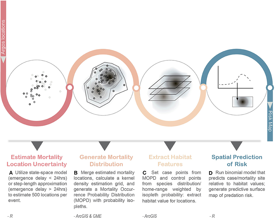
Figure 1. General work-flow for developing a spatially explicit risk map of predation for marine top predators. Inputs into the workflow include Argos location data from pop-up transmitters (e.g., LHX tags, miniPATs) and external Satellite Data Recorders (SDRs). This approach captures the uncertainty of emergence location for mortality events (A,B) and incorporates it into the determination of case and control points used in subsequent habitat modeling of risk (C,D). Steps were conducted in program R, ArcGIS, and Geospatial Modeling Environment (GME v0.7.2.0).

Methods

Animal Capture and Tagging

Over the past 40 years, the endangered, western population segment (west of 144° W) of the SSL has declined to ~20% of peak population levels documented in the 1970s. It has been posited that the lack of recovery in the western population segment is associated with the quality (Fritz and Hinckley, 2005) and availability of food resources (Holmes et al., 2007), changing ocean conditions (Trites et al., 2007), and increased predation pressure (Springer et al., 2003; Horning and Mellish, 2012). As part of large-scale efforts to tease apart the effects of predation on this species, from 2003 to 2014, seventy SSLs (male n = 41, female n = 29) between 13 and 25 months of age were captured in Prince William Sound (60° N 148° W) and Resurrection Bay, Alaska (60° N 149.30° W). The animals were transported to the Alaska SeaLife Center (ASLC) after capture, and 45 animals (male n = 28, female n = 17) underwent surgical implantation of LHX tags between 2005 and 2014 (Horning et al., 2008). Detailed information on capture, handling, biosampling and instrumentation techniques are described in detail in (Mellish et al., 2006, 2007; Horning et al., 2008, 2017a; Thompton et al., 2008). All animals were subsequently released in Resurrection Bay with external Satellite Data Recorders (SDRs, Wildlife Computers, Redmond, WA) following 1-6 weeks of postoperative monitoring in captivity under veterinary care. LHX tag implantation and temporary captivity was found to have no significant effect on animal diving behavior post-release (Mellish et al., 2007; Thompton et al., 2008) and there was no evidence of reduced post-release survival through the age of five years due to LHX implantation surgery or temporary captivity (Shuert et al., 2015).

Estimating Mortality Events Locations

Mortality events were detected through state transitions in the LHX tags, indicating temperatures outside a user-defined physiological temperature range (i.e., first state transition; Horning and Hill, 2005). An acute death (e.g., dismemberment) such as an attack by a predator leads to: (1) the immediate extrusion of implanted tags and rapid cooling in the ambient medium or; (2) the tag getting lodged and more gradually cooling within chunks of smaller body parts (Horning and Mellish, 2009). A non-traumatic event other than predation should lead to algor mortis (slow cooling of an intact body) and delayed tag extrusion after the body slowly decomposes (Horning and Mellish, 2009). Date and time of death is therefore determined, stored and later transmitted with a 30 min resolution following a second state transition (i.e., sensing of light and air) indicating tag extrusion.

Once a tag emerges from the body of a deceased animal and senses light and air, satellite transmissions are initiated within 24 h. Transmitted data include body temperature and light data, and a mortality date/timestamp. Locations are not included in the data stream, as LHX tags have no means to calculate their position. Instead, the Argos system calculates geographic location estimates from the Doppler frequency shift across multiple sequential transmissions received during a single satellite pass. Individual location estimates are assigned an accuracy in the form of one of 7 location classes (LC 3, 2, 1, 0, A, B, and Z), ranging from <150 m (LC 3) to > 1.5 km (LC B), and class Z has no accuracy assigned (Hays et al., 2001). To maximize the probability of the return of at least some transmissions, tags were programmed to only commence transmissions at 12:00 noon Alaska Standard Time. This could introduce a varying delay between the second state transition and onset of transmissions of 1–24 h. Since tags can drift considerably during this time between transmissions, the accuracy of the estimated mortality location may decrease with delayed uplinks. Additionally, multiple successful uplinks within a single satellite pass are required to improve location accuracy which may not be immediately attainable in rough or choppy surface conditions and can further delay tag location estimates post-mortem.

Out of the 45 LHX tagged animals, 20 mortalities were detected between November 2005-December 2018 (Horning and Mellish, 2014; Horning et al., 2017b; Bishop et al., 2019). Two of the detected mortalities yielded insufficient data to determine the proximate cause of mortality and were excluded from analysis. The remaining 18 individual mortalities were characterized as predation (Horning and Mellish, 2014). We found that the lag between tag extrusion and the first calculated location estimate ranged from 1 h to several days. Five of these 18 individuals had spatial event data associated with very large uncertainties due to delayed uplinks (> 5 days) to the ARGOS satellite system after extrusion (Brown et al., 2019). These events were excluded from our spatial analysis (Table 1).

TABLE 1

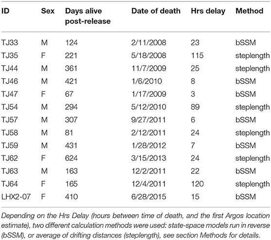
Table 1. Descriptions of predation events detected via Life History (LHX) tags for each juvenile Steller sea lion.

LHX Tag Location Processing

To estimate the actual emergence location (coinciding in time with the mortality event), we applied a modified, continuous-time state-space model (SSM) in the R (v3.4.0) package crawl (Johnson et al., 2008) to all available post-emergence location data. The standard crawl models use Bayesian filters to estimate the current location conditional on preceding locations (Särkkä, 2013), which improves output accuracy as all available data are utilized. Here, we ran the model in reverse to use all available post-emergence spatial and location quality information. The final location obtained was reassigned as the first location for the model, and all subsequent steps were backtracked in time, such that, the first actual location estimate obtained by Argos was used as the last location in the model. The development and validation of this backward-SSM (bSSM) approach is described in detail in Brown et al. (2019).

Model output was then further generated backwards to the time of tag emergence, to extrapolate an emergence location (Brown et al., 2019). This process was repeated 500 times generating 500 emergence locations/tag (Figure 2A). To account for locations on land, we ran the estimated emergence locations through {fixpath} in crawl, a function which moves points on land to the closest sea location along the path trajectory (Johnson et al., 2008). Brown et al. (2019) found that accuracy of extrapolated emergence locations substantially decreased using the backwards SSM approach when the time lag between emergence and first Argos location estimates was > 24 h. Thus, we only used the backward SSM approach for tags (n = 7, Table 1) that yielded an Argos location within 24 h from emergence. For tags with location delays > 24 h (n = 6, Table 1), we used an alternate approach. We averaged the distance between consecutive locations for the entire time the tag was transmitting at the surface to estimate an average drifting distance (steplength). We then applied that average drift distance to the first quality emergence location (LC 2-3) to create a buffer surrounding that location (Figure 2B). We assumed that the predation event occurred within that buffered area, and 500 points were randomly generated within each polygon.

FIGURE 2

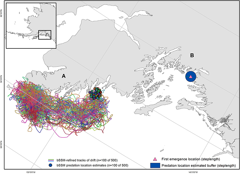
Figure 2. Two examples of mortality location and uncertainty estimation methods. (A) For data with < 24 h uplink delay, state-space model simulations were run in reverse (bSSM), utilizing all available Argos location estimates post-emergence to generate a predicted emergence (predation) location. For each observed predation event, 500 bSSM simulations were run, resulting in 500 predation location estimates. A subset of LHX2_07's bSSM simulation tracks are shown here (n = 100), with estimated predation locations clustered around the Chiswell Islands. (B) For data with > 24hr uplink delay, a step-length calculation generated a buffer around the emergence location within which predation was estimated to have occurred. The first emergence location for TJ44, and estimated predation location buffer in Prince William Sound are shown.

Generating Case/Control Locations for Habitat Modeling

Because the output locations from the extrapolated, bSSMs and within the steplength buffers are equally weighted regardless of uncertainty, we used a multi-step process for extracting habitat feature data associated with predation events that maximized the use of available data from known predation locations, and incorporated the variation in the spatial uncertainty (Figure 1). First, in ArcGIS 10.6 (ESRI), we merged the estimated emergence locations that were output from each of the SMMs and the randomly generated points within each step-length buffer (n = 6500). We used a fixed kernel density estimator (kde) with cross validation bandwidth (1 km × 1 km) to generate a Mortality Occurrence Probability Distribution (MOPD) in Geospatial Modeling Environment v 0.7.2.0. The MOPD represented the case space, or the space where predation events most likely occurred. To extract habitat data associated with case space, we first calculated the area in each isopleth (0.10–0.95, Table 2). Then, starting with a density of 5 case-locations per km² in the 0.10 isopleth, we distributed points (randomized spatially in ArcGIS) in each subsequent isopleth so that the resulting density was in proportion with the isopleth's associated probability (Table 2). This resulted in a dataset of 115 case/mortality locations. To generate comparable control locations, or locations describing habitat juvenile SSLs utilize while alive, we applied the same density-weighting approach to generate points across the juvenile SSL Utilization Distribution (UD) published in Bishop et al. (2018) generated from satellite movement tracking data locations in this region (n = 84) during the same temporal period. This resulted in a dataset of 1,000 control locations (Table 2).

TABLE 2

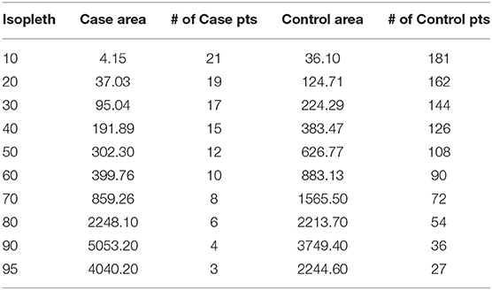
Table 2. The area (km²) and number of points generated per isopleth in the Case mortality occurrence probability distribution and Control utilization distribution based on a starting density of 5 points per km², with subsequent weighting proportionate to the isopleth's associated probability.

Generating Spatially-Explicit Risk Map

We used generalized additive models (GAMs) to predict the probability of predation spatially, relative to static habitat features. The GAM was fit using a binomial distribution with a logit link function and residual maximum-likelihood estimator with the mgcv package (Wood, 2006) in R (v.3.5.3). We restricted the number of knots (k = 5) to avoid overfitting. We used a case-control design to predict the relative probability of a predation location (1) compared to locations randomly generated within the full extent of the SSL population UD (0). Using standard tools in ArcGIS, we extracted several environmental covariates at each case and control location to depict variation in risk across our study area, including depth (m) and bathymetric-slope (degrees) (Lim et al., 2011), and distance to known SSL haulouts (km, Fritz et al., 2015) (Figure 3). Depth may represent predator-specific predation risk since transient killer whales, one of the primary hypothesized predators of SSL (Loughlin and York, 2000), hunts near the surface, while predation by Pacific sleeper sharks (Somniosus pacificus), another hypothesized predator (Loughlin and York, 2000; Frid et al., 2009; Horning and Mellish, 2014) is predicted to be very low near the ocean surface but increase in probability with depth (Frid et al., 2009). We used bathymetric slope as a proxy for gradient in depth and biomass production (Aydin et al., 2002). Depth and bathymetric slope can influence foraging decisions (Baylis et al., 2015) and spatial distribution of sea lions (Aarts and Brasseur, 2008) and can be used as a proxy for risk-reward tradeoffs. Distance to known SSL haulouts (Fritz et al., 2015) was used as a surrogate for perceived low-risk habitat.

FIGURE 3

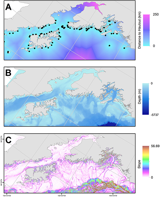
Figure 3. Habitat variables included as predictors of predation in our study area, the Gulf of Alaska: (A) distance to Steller sea lion haulout or rookery (km; haulouts/rookeries denoted as black points; Fritz et al., 2015), (B) depth (m), and (C) slope derived from bathymetry (Lim et al., 2011).

Potential models were assessed based on weighted Akaike Information Criterion (AIC), in addition to area under the curve (AUC) cross-validation statistics. AUC statistics are calculated from receiver operating characteristic (ROC) curves which use the inflection point to maximize the true positive rate, while minimizing the false-positive rate (DeLong et al., 1988). We calculated ROC curves and AUC statistics using the ROCR package in R (1.0-7). The spatial distribution of predation risk was visualized in ArcMap using the best model, with spatial extent constrained to the observed SSL control dataset.

Results

Spatial Distribution of Mortality Events

Predation events occurred across the Gulf of Alaska, including Prince William Sound, the Kenai Fjords region, lower Cook Inlet and west of Kodiak Island (Figure 4A). Of the 13 events analyzed here, the time between mortality and first computed locations obtained via satellite uplinks ranged from 3 to 120 h (Table 1). Areas of bSSM-derived uncertainty polygons ranged from (0.27–3729.77 km²), and the areas of steplength derived uncertainty polygons ranged from (170.13–9245.73 km²). When combined into a MOPD, the 10–95% isopleths for the case/mortalities combined covered a total area of 13,230.9 km² (Table 2, Figures 4A,B). The control UD (Bishop et al., 2018) covered a similar area, 12,051.6 km² (Table 2, Figures 4C,D). The proportion of high probability areas, isopleths 10–50%, was greater for the control UD (11.6%) relative to the case MOPD (4.7%).

FIGURE 4

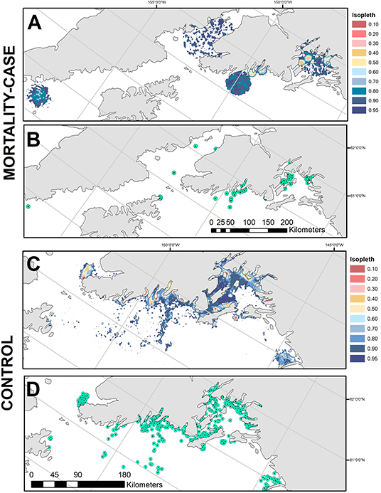
Figure 4. (A) The mortality occurrence probability distribution, and (B) the generated case locations (n = 100) from which habitat features were extracted. (C) The control utilization distributions from Bishop et al. (2018), and (D) the generated control locations (n = 1,000), from which habitat features were extracted.

Spatial Prediction of Risk

The model with the highest empirical support relating the probability of predation to habitat features included all variables considered: depth, slope, distance to haulout (Table 3). Slope and distance to SSL haulout variables were characterized by non-linear relationships (Table 3, Figure 5). Our final GAM showed predation was less likely to occur for slope values between 2 and 10° than for steeper slopes (Figure 5). As distance from SSL haulouts increased (0–20 km) predation likelihood increased, but then decreased at intermediate distances from SSL haulouts (40–80 km). Predation likelihood increased linearly in areas with deeper bathymetry, but so did model uncertainty (Figure 5). Based on the AUC score of the final model (0.74, Supplemental Figure 1), model accuracy was good in the predictions of the spatial distribution of predation risk for Steller sea lions (Table 3, Figure 6).

TABLE 3

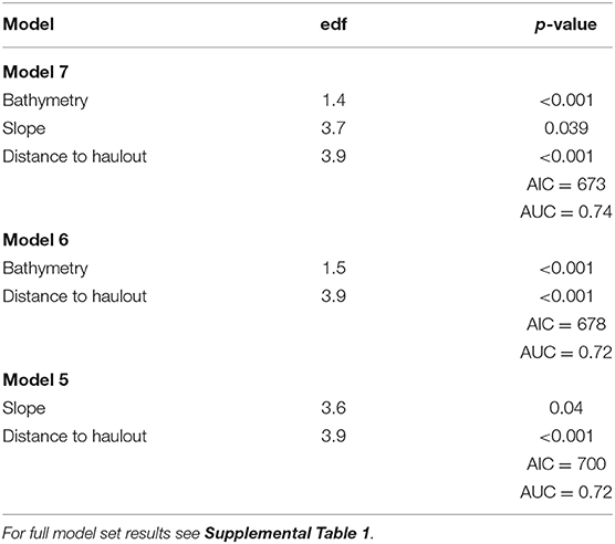
Table 3. Top three candidate model summaries estimated by generalized additive models predicting probability of predation including Akaike Information Criterion (AIC) and area under the curve (AUC) statistics.

FIGURE 5

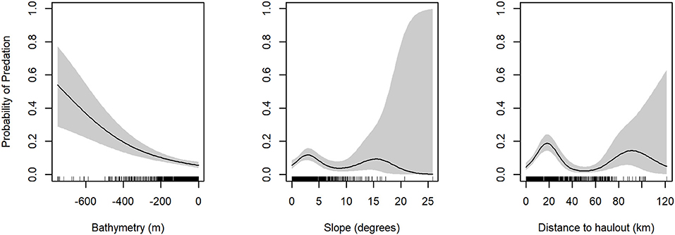
Figure 5. Partial plots for generalized additive models for predation presence/absence variables. Probability of Predation is on the y-axis and environmental variable is on the x-axis. Standard error is shaded in gray.

FIGURE 6

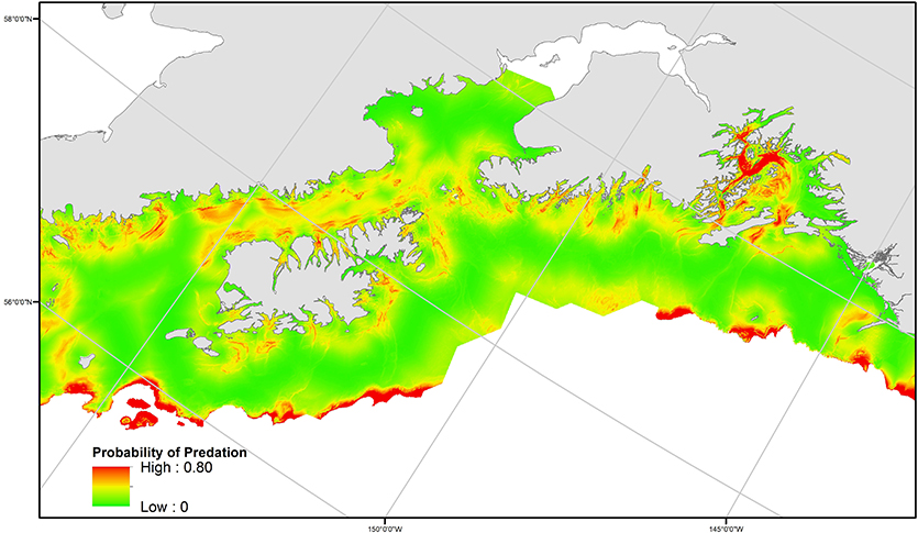
Figure 6. Spatial distribution of predicted predation probability, as estimated from the best generalized additive model based on the relationship to distance to haulout, bathymetry (depth), and slope. The spatial extent is constrained by habitat (bathymetry and distances from haulouts) juvenile SSLs were associated with* in control data. *Note, association with bathymetry refers to the specific depth at a SSL movement location, not SSL usage of the vertical water column.

Discussion

The approach we introduce here allows the integration of spatially explicit data from multiple telemetry and remote sensing sources with differing degrees of spatio-temporal uncertainty. Furthermore, this process incorporates quantitative estimates of uncertainty that are based on actual data collected through individual telemetry devices. Through our novel approach, spatially explicit risk maps can be generated through association between predation locations and static habitat features (Figure 1). Our case study, utilizing predation events of juvenile SSLs (n = 13) in the Gulf of Alaska, highlights the effectiveness of this method to explore habitat features associated with direct predation risk. We found evidence that juvenile SSL predation events were associated with habitats characterized by greater depths and moderate distances from rookeries.

Our multi-step process to characterize habitat associated with predation events maximizes the use of all available telemetry data; however, there are still some limitations to this system. LHX tags are the first available technology to detect, locate and characterize mortality, and specifically in their ability to identify predation events, in marine homeotherms with spatio-temporally unrestricted monitoring effort (Horning and Hill, 2005; Horning and Mellish, 2009). These tags were designed along a hierarchical set of functionalities. The top priority was given to maximizing post-mortem data return probability, whereas mortality event location determination was assigned a low priority. In the Argos telemetry system, locations are calculated from the Doppler frequency shift of multiple sequential transmissions received by one receiving satellite during a single pass—location information is not included in the transmitted data stream. The quality associated with a subsequently calculated location is linked to the number of transmissions received during a single satellite pass. If transmissions are widely spaced in time, it is also possible to transmit data without ever obtaining locations. In a simplex transmission system such as Argos, data need to be transmitted with a given level of redundancy to achieve a given probability of being received. To increase the likelihood of obtaining quality location estimates, the transmit rate should be increased. However, this could reduce the likelihood of receiving any transmissions if all occur in a short time under adverse conditions (e.g., bad sea state). Furthermore, the heuristic algorithm used to determine tag state and initiate transmissions under optimal conditions was programmed to evaluate light sensor data only once per 24 h, which introduced variable delays between time of death and onset of transmissions. To address these constraints, LHX tags were designed along a hierarchical set of functionalities. This was done to maximize the probability of receiving at least one post-mortem transmission from a tag (sufficient to confirm death), at the expense of a low probability of an early, higher quality location.

In addition to the programming limitations imposed by LHX tags, our case study was limited by sample size. Initial applications of LHX tags in 45 juvenile SSLs in the Gulf of Alaska revealed at least 18 of 20 detected mortalities were attributed to predation, suggesting a proportion of juvenile sea lion mortalities due to predation in the Kenai Fjords—Prince William Sound region of 0.917 (95% C.I. 0.78–1.0, as per Horning and Mellish, 2012, 2014). Due to the aforementioned programming limitations, we only had location estimates for 13 of these predation events, and spatial uncertainty related to these events was highly variable. This limited our ability to explore seasonal patterns or dynamic habitat features of interest, those likely correlated with resource distribution; although, in most cases, these features (e.g., sea surface temperature, chlorophyll a) typically have a spatial resolution that is too low in the higher latitudes and fjord geography of our study area. Such variables could easily be incorporated into this method to refine habitat features associated with risk in other systems, or to explore seasonal differences in risk from greater sample sizes.

Despite limitations in sample size and a lack of opportunity to consider dynamic habitat features, some patterns emerged from the analysis of SSL predation events. The predominant pattern was that deeper bathymetry was associated with increased predation risk. However, this effect increased over water depths well in excess of the median of maximum dive depths of juvenile SSL (126.1 m, Thompton et al., 2008). Without a concurrent analysis of dive depths from the external transmitters or depth information associated with mortality events, it seems very unlikely that sea lions were using the full range of available bathymetry, and more likely were spending time closer to the surface over greater depths. Pacific sleeper sharks are a hypothesized predator of juvenile SSLs with indirect evidence of predation from analysis of telemetry data (Horning and Mellish, 2014). They are thought to be opportunist predator-scavengers that spend much time over deeper bathymetry and at depths beyond median sea lion dive depths (Thompton et al., 2008). They do however range closer to the surface at night (Hulbert et al., 2006) where opportunistic encounters with sea lions may lead to predation.

Distance from rookeries and haulouts had a slight positive association with predation risk increasing up to 20 km, but at greater distances the risk diminished again. This finding may appear to contradict the observation by Bishop et al. (2019) of slightly elevated predation risk for individuals with increased haulout times during summer, which must occur near rookeries and haulouts, even while overall risk was lower in summer than winter. This disconnect may be due to the differences in temporal scales across studies. In our current study, sample size limited exploration of seasonal differences habitats associated with predation, which may mask the predation risk associated with sea lion behaviors in the summer. However, summer haulout behavior is driven by increased social interactions in rookeries during breeding, and may be concomitant with increased entry into and exit from water. Thus, while overall time dry may increase, time spent in the waters near a rookery is likely also higher, rather than foraging at more distant locations, which could concentrate sea lions for predators. Previous work has found that average annual predation by transient killer whales on SSLs (mainly pups and juveniles) at one rookery in our study region accounted for 3–7% of the local summer seasonal population of sea lions (Ford et al., 1998; Maniscalco et al., 2007). Slope of bathymetry was also associated with predation risk, which was highest at comparably shallow angles around 2–3 degrees (Figure 5). Most shorelines in the region are steep, and therefore this effect matches the shape of the distance pattern, and probably reflects the same root cause.

Overall, between the present study and Bishop et al. (2019), the observed diving, haulout, spatial and habitat use associated with resource-risk trade-offs are consistent with a mix of at least two predator types—transient killer whales and Pacific sleeper sharks, as proposed and theoretically modeled by Frid et al. (2009). Interestingly, the observations by Bishop et al. (2019) that may indirectly suggest closer-to-rookery predation in the summer were derived primarily from telemetered sea lion dive behavior data and were informed by predation event timing, but not location. The positive association of predation risk with deeper bathymetry, and distance from rookeries we report here were derived from predation event telemetry timing and location, and was only spatially constrained by telemetered sea lion movement. Both reflect consumptive effects, presumably from a mix of predators, and provide information about the extrinsic and intrinsic factors associated with risks for juvenile Steller sea lions. This highlights the complementary nature of the two types of telemetry used in this study, external behavioral tracking tags, and internal, predation detecting.

As marine ecosystems continue to experience rapid changes, it will be critical to have methods for assessing inter-species interactions, particularly predator-prey interactions, in order to evaluate the potential impacts to ecosystem structure. Marine risk maps, linking habitat to predation probability, could provide insights into the biological connections in the ecosystem, be used to develop further hypotheses, or focus observational effort to spatial and temporal windows that are identified as being associated with risk. Though explored through a case-study on juvenile Steller sea lions, the process described here was designed to be applicable across a range of species and telemetry types already used in marine systems where mortality data-sources have a high degree of spatio-temporal uncertainty. Spatially explicit information on predation risk can also provide the framework for assessing non-consumptive effects of predation. Satellite telemetry data have provided evidence of non-consumptive effects of predators on prey species in open ocean systems including shifting movement (Westdal et al., 2017; Matthews et al., 2020) and habitat use patterns (Ferguson et al., 2010). For example, previous work has found that narwhal will shift habitat use closer to shore (Breed et al., 2017) and bowhead whales will select for heavy sea ice (Matthews et al., 2020) when killer whales are present. Studies that link these observations with data showing consumptive or direct mortality (e.g. kill sites) effects of predators on prey are lacking and can further enhance our understanding of how biophysical habitat characteristics influence predation success and resource trade-offs.

Data Availability Statement

The data analyzed in this study is subject to the following licenses/restrictions. All datasets generated for this study are available through the Wildlife Computers Data Portal, upon reasonable request from MH. Requests to access these datasets should be directed to Markus Horning, markush@alaskasealife.org.

Ethics Statement

The animal study was reviewed and approved by the Institutional Animal Care and Use Committees of the Alaska Sea Life Center (protocol numbers 02-015, 03-007, 05-002, 06-001, 08-005, and R10-09-04) and by the National Marine Fisheries Service (permit numbers 1034-1685, 1034-1887, 881-1890, 881-1668, 14335, and 14336).

Author Contributions

MH: conceived study and collected the data. AB, CB, and RS: analyzed the data. All authors wrote the manuscript and contributed to the interpretation of the data. All authors contributed to the article and approved the submitted version.

Funding

Data collection was supported by funding from North Pacific Research Board (NPRB) projects R1011, R1310, and the NOAA NA17FX1429 to MH. Data analysis was funded by NPRB R1512 and NSF award no. 1556495 to MH. The funders had no role in study design, data collection and analysis, decision to publish, or preparation of the manuscript.

Conflict of Interest

The authors declare that the research was conducted in the absence of any commercial or financial relationships that could be construed as a potential conflict of interest.

Acknowledgments

We thank all researchers and participants in the Transient Juvenile Steller sea lion project, specifically Principal Investigator, J. E. Mellish. We also thank our Alaska Department of Fish and Game collaborators involved in collecting the data which was incorporated into the previously published juvenile Steller sea lion utilization distribution; the output of which was used in this study. The data incorporated into this study was from projects carried out in strict compliance with all applicable animal care and use guidelines under the US Animal Welfare Act and approved as required under the US Marine Mammal Protection Act and the US Endangered Species Act by the National Marine Fisheries Service (permit numbers 1034-1685, 1034-1887, 881-1890, 881-1668, 14335, and 14336) and by the Institutional Animal Care and Use Committees of the Alaska Sea Life Center (protocol numbers 02-015, 03-007, 05-002, 06-001, 08-005, and R10-09-04).

Supplementary Material

The Supplementary Material for this article can be found online at: https://www.frontiersin.org/articles/10.3389/fmars.2020.576716/full#supplementary-material

References

Aarts, G. M., and Brasseur, S. M. (2008). Modelling Habitat Preference and Estimating the Spatial Distribution of Australian Sea Lions (Neophoca cinerea);” a First Exploration (No. C107/08). IMARES.

Google Scholar

Aydin, K. Y., Lapko, V. V., Radchenko, V. I., and Livingston, P. A. (2002). A comparison of the eastern Bering and western Bering Sea shelf and slope ecosystems through the use of mass-balance food web models. NOAA Technical Memorandum NMFS-AFSC. 130.

Google Scholar

Baylis, A. M., Orben, R. A., Arnould, J. P., Peters, K., Knox, T., Costa, D. P., et al. (2015). Diving deeper into individual foraging specializations of a large marine predator, the southern sea lion. Oecologia 179, 1053–1065. doi: 10.1007/s00442-015-3421-4

PubMed Abstract | CrossRef Full Text | Google Scholar

Bishop, A., Brown, C., Rehberg, M., Torres, L., and Horning, M. (2018). Juvenile Steller sea lion (Eumetopias jubatus) utilization distributions in the Gulf of Alaska. Mov. Ecol. 6:6. doi: 10.1186/s40462-018-0124-6

PubMed Abstract | CrossRef Full Text | Google Scholar

Bishop, A. M., Dubel, A. K., Sattler, R., Brown, C. L., and Horning, M. (2019). Wanted dead or alive: characterizing likelihood of juvenile Steller sea lion predation from diving and space use patterns. End. Sp. Res. 40, 357–367. doi: 10.3354/esr00999

CrossRef Full Text | Google Scholar

Bleicher, S. S. (2017). The landscape of fear conceptual framework: definition and review of current applications and misuses. PeerJ 5:e3772. doi: 10.7717/peerj.3772

PubMed Abstract | CrossRef Full Text | Google Scholar

Breed, G. A., Matthews, C. J., Marcoux, M., Higdon, J. W., LeBlanc, B., Petersen, S. D., et al. (2017). Sustained disruption of narwhal habitat use and behavior in the presence of Arctic killer whales. Proc. Natl. Acad. Sci. U.S.A. 114, 2628–2633. doi: 10.1073/pnas.1611707114

PubMed Abstract | CrossRef Full Text | Google Scholar

Brown, C. L., Horning, M., and Bishop, A. M. (2019). Improving emergence location estimates for Argos pop-up transmitters. Anim. Biotelemetry 7:4. doi: 10.1186/s40317-019-0166-6

CrossRef Full Text | Google Scholar

DeLong, E. R., DeLong, D. M., and Clarke-Pearson, D. L. (1988). Comparing the areas under two or more correlated receiver operating characteristic curves: a nonparametric approach. Int. Biometric Soc. 44, 837–845. doi: 10.2307/2531595

CrossRef Full Text | Google Scholar

Ferguson, S. H., Dueck, L., Loseto, L. L., and Luque, S. P. (2010). Bowhead whale Balaena mysticetus seasonal selection of sea ice. Mar. Ecol. Prog. Ser. 411 285–297. doi: 10.3354/meps08652

CrossRef Full Text | Google Scholar

Ford, J. K. B., Ellis, G. M., Morton, A. B., and Balcomb, K. C. III. (1998). Dietary specialization in two sympatric populations of killer whales (Orcinus orca) in coastal British Columbia and adjacent waters. Can. J. Zool. 76, 1456–1471. doi: 10.1139/cjz-76-8-1456

CrossRef Full Text | Google Scholar

Frid, A., Burns, J., Baker, G. G., and Thorne, R. E. (2009). Predicting synergistic effects of resources and predators on foraging decisions by juvenile Steller sea lions. Oecologia 158, 775–786. doi: 10.1007/s00442-008-1189-5

PubMed Abstract | CrossRef Full Text | Google Scholar

Fritz, L., Sweeney, K., Towell, R., and Gelatt, T. (2015). Steller Sea Lion Haulout and Rookery Locations in the United States for 2016-05-14 (NCEI Accession 0129877). V 2.3 NOAA. National Centers for Environmental Information.

Fritz, L. W., and Hinckley, S. (2005). A critical review of the regime shift - “Junk Food” - nutritional stress hypothesis for the decline of the western stock of steller sea lion. Mar. Mam. Sci. 21 476–518. doi: 10.1111/j.1748-7692.2005.tb01245.x

CrossRef Full Text | Google Scholar

Hammerschlag, N., Broderick, A. C., Coker, J. W., Coyne, M. S., Dodd, M., Frick, M. G., et al. (2015). Evaluating the landscape of fear between apex predatory sharks and mobile sea turtles across a large dynamic seascape. Ecology 96, 2117–2126. doi: 10.1890/14-2113.1

PubMed Abstract | CrossRef Full Text | Google Scholar

Hays, G. C., Åkesson, S., Godley, B. J., Luschi, P., and Santidria, P. (2001). The implications of location accuracy for the interpretation of satellite-tracking data. Anim. Behav. 61, 1035–1040. doi: 10.1006/anbe.2001.1685

CrossRef Full Text | Google Scholar

Holmes, E. E., Fritz, L. W., York, A. E., and Sweeney, K. (2007). Age-structured modeling reveals long-term declines in the natality of western Steller sea lions. Ecol. Appl. 17, 2214–2232. doi: 10.1890/07-0508.1

PubMed Abstract | CrossRef Full Text | Google Scholar

Hooker, S. K., Biuw, M., McConnell, B. J., Miller, P. J. O., and Sparling, C. E. (2007). Bio-logging science: logging and relaying physical and biological data using animal-attached tags. Deep Sea Res. 2, 177–182. doi: 10.1016/j.dsr2.2007.01.001

CrossRef Full Text | Google Scholar

Horning, M., Haulena, M., Rosenberg, J. F., and Nordstrom, C. (2017a). Intraperitoneal implantation of life-long telemetry transmitters in three rehabilitated harbor seal pups. BMC Vet. Res. 13:139. doi: 10.1186/s12917-017-1060-1

PubMed Abstract | CrossRef Full Text | Google Scholar

Horning, M., Haulena, M., Tuomi, P. A., Mellish, E. J. A., Goertz, E. C., Woodie, K., et al. (2017b). Best practice recommendations for the use of fully implanted telemetry devices in pinnipeds. Anim. Biotelemetry 5:13. doi: 10.1186/s40317-017-0128-9

CrossRef Full Text | Google Scholar

Horning, M., Haulena, M., Tuomi, P. A., and Mellish, J. A. (2008). Intraperitoneal implantation of life-long telemetry transmitters in Otariids. BMC Vet. Res. 4:51. doi: 10.1186/1746-6148-4-51

PubMed Abstract | CrossRef Full Text | Google Scholar

Horning, M., and Hill, R. (2005). Designing an archival satellite transmitter for life-long deployments on oceanic vertebrates: the life history transmitter. IEEE J. Ocean Eng. 30, 807–817. doi: 10.1109/JOE.2005.862135

CrossRef Full Text | Google Scholar

Horning, M., and Mellish, J. A. (2012). Predation on an upper trophic marine predator, the steller sea lion: evaluating high juvenile mortality in a density dependent conceptual framework. PLoS ONE 7:e30173. doi: 10.1371/journal.pone.0030173

PubMed Abstract | CrossRef Full Text | Google Scholar

Horning, M., and Mellish, J. E. (2009). Spatially explicit detection of predation on individual pinnipeds from implanted post-mortem satellite data transmitters. Endanger. Species Res. 10, 135–143. doi: 10.3354/esr00220

CrossRef Full Text | Google Scholar

Horning, M., and Mellish, J. E. (2014). In cold blood: evidence of Pacific sleeper shark (Somniosus pacificus) predation on Steller sea lions (Eumetopias jubatus) in the Gulf of Alaska. Fish. Bull. 112, 297–310. doi: 10.7755/FB.112.4.6

CrossRef Full Text | Google Scholar

Horodysky, A. E., and Graves, J. E. (2005). Application of pop-up satellite archival tag technology to estimate post release survival of white marlin (Tetrapturus albidus) caught on circle and straight shank (“J”) hooks in the western North Atlantic recreational fishery. Fish. Bull. 103, 84–96. Available online at: https://scholarworks.wm.edu/vimsarticles/1760

Google Scholar

Hulbert, L. B., Sigler, M. F., and Lunsford, C. R. (2006). Depth and movement behaviour of the Pacific sleeper shark in the north-east Pacific Ocean. J. Fish Biol. 69, 406–425. doi: 10.1111/j.1095-8649.2006.01175.x

CrossRef Full Text | Google Scholar

Hussey, N. E., Kessel, S. T., Aarestrup, K., Cooke, S. J., Cowley, P. D., Fisk, A. T., et al. (2015). Aquatic animal telemetry: a panoramic window into the underwater world. Science. 348, 1–10. doi: 10.1126/science.1255642

PubMed Abstract | CrossRef Full Text | Google Scholar

Johnson, D. S., London, J. M., Lea, M. A., and Durban, J. W. (2008). Continuous-time correlated random walk model for animal telemetry data. Ecology 89, 1208–1215. doi: 10.1890/07-1032.1

PubMed Abstract | CrossRef Full Text | Google Scholar

Kerstetter, D. W., Luckhurst, B. E., Price, E., and Graves, J. E. (2003). Pop-up satellite archival tags to demonstrate survival of blue marlin (Makaira nigricans) released from pelagic longline gear. Fish. Bull. 101, 939–948. Available online at: https://nsuworks.nova.edu/occ_facarticles/543

Google Scholar

Kohl, M. T., Stahler, D. R., Metz, M. C., Forester, J. D., Kauffman, M. J., Varley, N., et al. (2018). Diel predator activity drives a dynamic landscape of fear. Ecol. Monogr. 88, 638–352. doi: 10.1002/ecm.1313

CrossRef Full Text | Google Scholar

Laundré, J. W., Hernández, L., and Altendorf, K. B. (2001). Wolves, elk, and bison: reestablishing the “landscape of fear” in Yellowstone National park, U.S.A. Can. J. Zool. 79, 1401–1409. doi: 10.1139/z01-094

CrossRef Full Text | Google Scholar

Lendrum, P. E., Northrup, J. M., Anderson, C. R., Liston, G. E., Aldridge, C. L., Crooks, K. R., et al. (2017). Predation risk across a dynamic landscape: effects of anthropogenic land use, natural landscape features, and prey distribution. Landsc. Ecol. 33, 157–170. doi: 10.1007/s10980-017-0590-z

CrossRef Full Text | Google Scholar

Lim, E., Eakins, B. W., and Wigley, R. (2011). Coastal Relief Model of Southern Alaska: Procedures, Data Sources and Analysis, NOAA Technical Memorandum NESDIS NGDC-43. Available online at: http://www.ngdc.noaa.gov/mgg/coastal/s_alaska.html (accessed August 22, 2011).

Google Scholar

Lima, S. L., and Dill, L. M. (1990). Behavioral decisions made under the risk of predation: a review and prospectus. Can. J. Zool. 68, 619–640. doi: 10.1139/z90-092

CrossRef Full Text | Google Scholar

Lone, K., Loe, L. E., Gobakken, T., Linnell, J. D. C., Odden, J., Remmen, J., et al. (2014). Living and dying in a multi-predator landscape of fear: roe deer are squeezed by contrasting pattern of predation risk imposed by lynx and humans. Oikos 123, 641–651. doi: 10.1111/j.1600-0706.2013.00938.x

CrossRef Full Text | Google Scholar

Loughlin, T. R., and York, A. E. (2000). An accounting of the sources of Steller sea lion, Eumetopias jubatus, mortality. Mar. Fish. Rev. 62, 40–45. Available online at: http://aquaticcommons.org/9764/1/mfr6242.pdf

Google Scholar

Maniscalco, J. M., Matkin, C. O., Maldini, D., Calkins, D. G., and Atkinson, S. (2007). Assessing killer whale predation on Steller sea lions from field observations in Kenai Fjords, Alaska. Mar. Mamm. Sci. 23, 306–321. doi: 10.1111/j.1748-7692.2007.00103.x

CrossRef Full Text | Google Scholar

Matthews, C. J., Breed, G. A., LeBlanc, B., and Ferguson, S. H. (2020). Killer whale presence drives bowhead whale selection for sea ice in Arctic seascapes of fear. Proc. Nat. Acad. Sci. 117, 6590–6598. doi: 10.1073/pnas.1911761117

PubMed Abstract | CrossRef Full Text | Google Scholar

Mellish, J. A. E., Calkins, D. G., Christen, D. R., Horning, M., Rea, L. D., and Atkinson, S. K. (2006). Temporary captivity as a research tool: comprehensive study of wild pinnipeds under controlled conditions. Aq. Mam. 32, 58–65. doi: 10.1578/AM.32.1.2006.58

CrossRef Full Text | Google Scholar

Mellish, J. A. E., Thomton, J., and Horning, M. (2007). Physiological and behavioral response to intra-abdominal transmitter implantation in Steller Sea lions. J. Exp. Mar. Biol. Ecol. 351, 283–293. doi: 10.1016/j.jembe.2007.07.015

CrossRef Full Text | Google Scholar

Nielsen, J. K., Rose, C. S., Loher, T., Drobny, P., Seitz, A. C., Courtney, M. B., et al. (2018). Characterizing activity and assessing bycatch survival of Pacific halibut with accelerometer pop-up satellite archival tags. Anim. Biotelemetry 6:10. doi: 10.1186/s40317-018-0154-2

CrossRef Full Text | Google Scholar

Rayl, N. D., Bastille-Rousseau, G., Organ, J. F., Mumma, M. A., Mahoney, S. P., Soulliere, C. E., et al. (2018). Spatiotemporal heterogeneity in prey abundance and vulnerability shapes the foraging tactics of an omnivore. J. Anim. Ecol. 87, 874–887. doi: 10.1111/1365-2656.12810

PubMed Abstract | CrossRef Full Text | Google Scholar

Ripple, W. J., Estes, J. A., Schmitz, O. J., Constant, V., Kaylor, M. J., Lenz, A., et al. (2016). What is a trophic cascade? TREE 31, 842–849. doi: 10.1016/j.tree.2016.08.010

CrossRef Full Text | Google Scholar

Särkkä, S. (2013). Bayesian Filtering and Smoothing, Vol. 3. Cambridge, UK: Cambridge University Press.

Google Scholar

Seitz, A. C., Courtney, M. B., Evans, M. D., and Manishin, K. (2019). Pop-up satellite archival tags reveal evidence of intense predation on large immature Chinook salmon (Oncorhynchus tshawytscha) in the North Pacific Ocean. Canad. J. Fish. Aqu. Sci. 76, 1608–1615. doi: 10.1139/cjfas-2018-0490

CrossRef Full Text | Google Scholar

Shuert, C., Horning, M., and Mellish, J. A. E. (2015). The effect of novel research activities on long-term survival of temporarily captive Steller Sea lions (Eumetopias jubatus). PLoS ONE 10:e0141948. doi: 10.1371/journal.pone.0141948

PubMed Abstract | CrossRef Full Text | Google Scholar

Springer, A. M., Estes, J. A., van Vliet, G. B., Williams, T. M., Doak, D. F., Danner, E. M., et al. (2003). Sequential megafaunal collapse in the North Pacific Ocean: an ongoing legacy of industrial whaling? Proc. Natl. Acad. Sci. U.S.A. 100, 1223–1228. doi: 10.1073/pnas.1635156100

PubMed Abstract | CrossRef Full Text | Google Scholar

Thompton, J. D., Mellish, J. A. E., Hennen, D. R., and Horning, M. (2008). Juvenile steller sea lion dive behavior following temporary captivity. Endanger. Species Res. 4, 195–203. doi: 10.3354/esr00062

CrossRef Full Text

Trites, A. W., Miller, A. J., Alexander, M. A., Bograd, S. J., and Calder, J. A. (2007). Bottom-up forcing and the decline of Steller sea lions (Eumetopias jubatus) in Alaska: assessing the ocean climate hypothesis. Fish. Oceanogr. 1691, 46–47. doi: 10.1111/j.1365-2419.2006.00408.x

CrossRef Full Text | Google Scholar

Westdal, K. H., Davies, J., McPherson, A., Orr, J., and Ferguson, S. H. (2017). Behavioural changes in belugas (Delphinapterus leucas) during a killer whale (Orcinus orca) attack in southwest Hudson Bay. Can. Field-Nat. 130, 315–319. doi: 10.22621/cfn.v130i4.1925

CrossRef Full Text | Google Scholar

Williams, T. M., Estes, J. A., Doak, D. F., and Springer, A. M. (2004). Killer appetites: assessing the role of predators in ecological communities. Ecology 85, 3373–3384. doi: 10.1890/03-0696

CrossRef Full Text | Google Scholar

Wirsing, A. J., Heithaus, M. R., Frid, A., and Dill, L. M. (2008). Seascapes of fear: evaluating sublethal predator effects experienced and generated by marine mammals. Mar. Mam. Sci. 24, 1–15. doi: 10.1111/j.1748-7692.2007.00167.x

CrossRef Full Text | Google Scholar

Wood, S. N. (2006). Generalized Additive Models: An Introduction. R. Chapman and Hall/CRC.

Google Scholar