Spatio-Temporal Variations in Community Size Structure of Arctic Protist Plankton in the Fram Strait

1. Introduction

Noticeable oceanographic, biogeochemical, and ecological transformations have been documented for the Arctic Ocean. Along with trends in declining sea ice thickness and extent (Stroeve et al., 2012) and increasing sea surface temperature (SST) (Comiso and Hall, 2014), various changes in the marine Arctic ecosystem were recorded. These transformations include shifts in range, behavior, phenology, and abundance of marine mammals, birds, fish, plankton, and benthos (Wassmann et al., 2011). Therefore, describing and understanding plankton ecology and the underlying ecosystem dynamics involved in a changing Arctic Ocean has become a research focus for many marine scientists.

Regions of particular interest are the Barents Sea and the Fram Strait, because they are important gateways for warmer seawater entering the northern polar ocean, where cold Arctic Water meets warmer Atlantic Water. Long-term SST trends are difficult to ascertain in these regions, but observations indicate a warming and salinification due to an increased influence of Atlantic Water, which was reported for the Barents Sea by Barton et al. (2018). In the Fram Strait, the mean temperature of Atlantic Water increased linearly between 1997 and 2010, although no significant trend in volume transport was reported (Beszczynska-Möller et al., 2012). For more recent years, a study by Wang et al. (2020) indicates an increase in volume transport. The separation between Arctic Water and Atlantic Water in the Fram Strait is characterized by the northward flowing West Spitsbergen Current (WSC) and the East Greenland Current (EGC) that transports Polar water toward the south. The Fram Strait has been subject of various research in many disciplines over the past decades, as reviewed by Soltwedel et al. (2005, 2016). Of particular interest are variations in plankton composition in response to a changing influence of Atlantic Water in the Fram Strait, as they may entail subsequent effects on higher trophic levels and the biogeochemistry in Arctic regions north of Spitsbergen, e.g., the availability of fatty acids in large diatoms preyed by Arctic Calanus species (e.g., Falk-Petersen et al., 2009). For disclosing trophic interdependencies and eventually unraveling pathways of mass transfer to copepods, it is important to resolve changes in the community size structure of the microbial food web.

Cell size is regarded as key determinant of phytoplankton biology and it is interpreted as the master functional trait that affects plankton dynamics on cellular, population, and community levels (Chisholm, 1992; Raven, 1998; Litchman and Klausmeier, 2008; Finkel et al., 2010; Marañón, 2015). Size dependencies of bottom-up and top-down regulatory processes that determine size diversity can be subject to important trade-offs, e.g. between nutrient uptake and the vulnerability to grazing (Acevedo-Trejos et al., 2018). Ecosystem functioning and biogeochemical element cycling are known to be sensitive to the plankton community size structure (Falkowski et al., 1998). Understanding the major mechanisms that describe the coupling between autotrophic and heterotrophic activity within the microbial food web is critical for projecting future changes in biogeochemistry and trophic transfer in the Arctic (Thingstad et al., 2008). Three possible main pathways were discussed by Thingstad and Cuevas (2010), that describe how mineral nutrients can enter the plankton ecosystem and eventually determine the mass transfer to higher trophic levels, e.g., to copepods. The entry points are associated with osmotrophs of three distinct size ranges (i.e., heterotrophic bacteria, autotrophic flagellates, diatoms). A fourth pathway was investigated by Larsen et al. (2015), who introduced an additional size range by discriminating between large and small diatoms. Since all these pathways are size-dependent, temporal changes in autotrophic and heterotrophic plankton size spectra can be expected to disclose size ranges that inform about predator-prey interdependencies.

Is it important that we trace detailed changes in the plankton community structure, because some size ranges can be subject to predation, while yet other size ranges may act as “loopholes” (Bakun and Broad, 2003), with improved growth conditions and by escaping high predation rates (Irigoien et al., 2005). The size structure of a plankton community is commonly described as biomass spectrum (e.g., Rodriguez and Mullin, 1986; Sprules and Munawar, 1986) or size-abundance spectrum (y = logarithmic number of individuals vs. x = logarithmic size (e.g., Reul et al., 2005; Huete-Ortega et al., 2010, 2012). The y-intercept is ascribed to reflect total biomass, whereas the slope is interpreted as a measure of trophic efficiency. The slope is usually negative and it informs whether a community is dominated by larger (less negative) or smaller cells (more negative). It differs between coastal regions (−0.96, Huete-Ortega et al., 2010) and the open ocean (−1.15, Huete-Ortega et al., 2012), also increasing with latitude from −1.2 in the oligotrophic subtropical gyres to −0.6 in the North Atlantic (Barton et al., 2013). Deriving the y-intercept and the slope from abundance and cell size data can be ambiguous (Moreno-Ostos et al., 2015), because estimates of these two parameters can be collinear. Of potential interest are those size ranges that deviate from log-linear plankton size spectra, because they may reveal ecological details like distinctive size intervals of extensive predation as well as size ranges of reduced grazing pressure that can foster algal growth (loopholes) within the microbial food web.

Here we analyse plankton size spectra of the unicellular plankton community in the Fram Strait (Arctic Ocean) collected between 2016 and 2018. Rather than introducing individual size classes and imposing a linear (parametric) dependency between logarithmic cell concentration and logarithmic size, we derived non-parametric size spectra as Kernel Density Estimates (KDEs). Confidence intervals for the respective size spectra were determined by stochastic resampling, elaborating the KDE method as proposed by Schartau et al. (2010). The purpose of our extensive approach is to have details of the laborious microscopic measurements transferred to continuous size spectra of autotrophic and heterotrophic plankton in the size range between ≈ 1 μm (Micromonas) and ≈ 200 μm (large diatoms and tintinnids). We aim at identifying specific and robust patterns in the plankton community size structure of the microbial food web in the Arctic.

2. Materials and Methods

2.1. Description of the Sampling Site

The Fram Strait is considered a gateway to the Arctic Ocean. In the eastern part of the Fram Strait, warm and nutrient-rich water from the North-Atlantic is transported northwards with the West-Spitzbergen Current (WSC) (e.g., Beszczynska-Möller et al., 2012). The East-Greenland Current (EGC) transports colder and fresher water southwards in the western part (e.g., de Steur et al., 2009). Sea-ice cover in this region is variable. The western part is predominantly ice-covered throughout the year, the ice-cover in the north-eastern area varies seasonally while the south-eastern part remains permanently ice-free (Soltwedel et al., 2016). The sampling was conducted at the Fram Strait Long Term Ecological Research (LTER) observatory HAUSGARTEN (Figure 1) between 78°N–81°N and 5°W–11°E, a region that is characterized by the highly productive Marginal Ice Zone (Soltwedel et al., 2016). The sampling sites encompass cold Polar water of the EGC as well as of the warmer WSC.

FIGURE 1

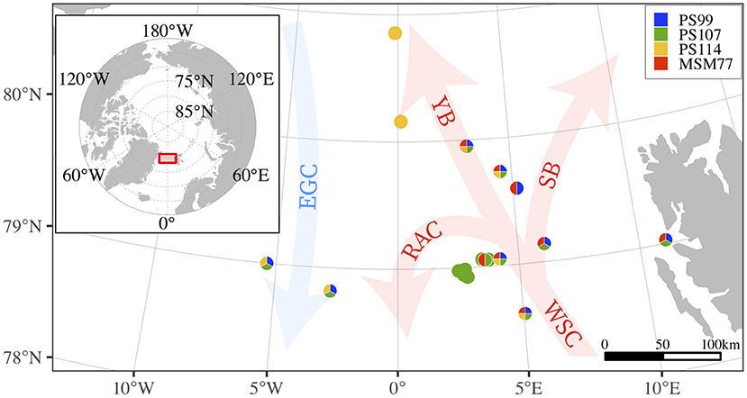
Figure 1. Location of the sampling site in the Fram Strait. Sampling stations are shown as dots, color-coded by the respective campaigns (Table 1 shows sampling time and depth ranges). Arrows show the main currents from the North-Atlantic (warm, red; WSC, West-Spitsbergen Current; RAC, Return Atlantic Current; YB, Yermak Branch; SB, Svalbard Branch) and the Arctic Ocean (cold, blue; EGC: East-Greenland Current), after Soltwedel et al. (2016).

2.2. Ship-Board Sampling

Plankton samples were collected during four cruises to the Fram Strait LTER Observatory (Table 1). Sea water samples were collected with a rosette sampler with 24 Niskin bottles (12 L). An attached CTD system (SEA-BIRD Instruments) recorded depth profiles for conductivity, temperature, and density. Respective plankton samples were fixed with 0.5–1% hexamine neutralized formaldehyde (final concentration) in brown glass bottles (200–250 mL) and stored in the dark until microscopic analyses (Edler, 1979). A total number of 60 samples were analyzed and cell sizes were measured in great detail.

TABLE 1

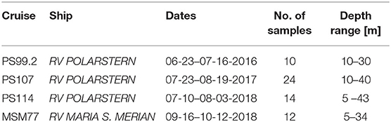
Table 1. Sampling campaigns to the HAUSGARTEN area in the Fram Strait (Arctic Ocean) during the years 2016–2018 recovered varying numbers of samples for microscopic community analyses.

2.3. Microscopic Community Composition and Size Measurements

Microscopic counting of phytoplankton and protozooplankton were conducted for 50 mL aliquots of each sample, following Utermöhl (1958) and Olenina et al. (2006). After a sedimentation period of at least 48 h, cells were identified and counted using an Utermöhl chamber and an inverted microscope (Axiovert 40 C) under 63x, 100x, 160x, 250x, and 400x magnification. Especially smaller species were only identified to genera. The corresponding cell lengths and widths were measured with a calibrated ocular micrometer (Zeiss). For further analyses, species were grouped by their trophic strategies, distinguishing between photo-autotrophy (phytoplankton) and heterotrophy (zooplankton).

The sample fixation can discolor chloroplasts, which hinders the determination of a cell's trophic strategy, when a precise identification is not available. Although common among protist plankton, mixotrophic cells could not be explicitly resolved. Green dinoflagellates were assigned to the group of photoautotrophs while their colorless counterparts were regarded as heterotrophic. A small fraction of micro- and nano-flagellates could not be unambiguously identified microscopically (mostly for cells with sizes smaller than 6 μm), which happened on average in 7.3% of all counts (resulting in 10.4% of the total cell concentration). Subject to these limitations, 50% of these cells were grouped as being photoautotrophic, and the remaining were assigned to the heterotrophic group. This assumption is based on our experience from previous measurements of samples taken in the Fram Strait, where the relative fractions between photoautrophs and heterotrophs in nanoflagellates varied between 30 and 70%. A study by Sherr et al. (2003) supports our assumption. In general, during spring more photoautotrophic forms were observed, whereas in summer we had found heterotrophic forms that prevailed. In our samples, most of the small flagellates were identifiable such as the often dominating autotrophic Phaeocystis spp. single cells with cell sizes between 2 and 6 μm.

2.4. Resampling of Cell Counts and Size Measurements

When comparing individual size spectra, the consideration of inherent methodological uncertainties is helpful. This includes uncertainties in counts, as well as the precision of microscopic measurements of cell length and width. The former involves the sample volume and the microscopic area (field of view) scanned for counting, whereas the latter depends on the microscopic magnification. To account for such uncertainties, we followed the bootstrapping approach described in Schartau et al. (2010), by analysing ensembles of resample datasets. The generation of resample datasets was done in two consecutive steps. First, we resampled cell counts. In a second step, we assigned resampled cell lengths and widths to the respectively resampled counts.

Resample cell counts were obtained by randomly drawing from a Poisson probability distribution with an expected value λ that was equal to the observed number of cell counts, which had been summarized before according to cell taxonomy and size. This way we considered uncertainties in counting, which becomes particularly relevant in cases of finding few counts of a specific species/taxon of one particular size. Furthermore, a single count in a sub sample of 50 mL was regarded as a rare event and it is associated with a large uncertainty when upscaling it to a concentration (abundance in units cells L⁻¹). The consideration of a Poisson probability distribution for resampling counts is meaningful in this respect. For example, the probability of resampling an observed single count (λ = 1) as P(k = 1) = P(k = 0) ≈ 0.37, meaning that the probability of finding or missing such rare event is equal. Capturing two counts of identical size is also possible, although the probability reduces to P(k = 2) ≈ 0.18. The probability of finding three or more counts decreases further accordingly. Resampled cell counts were eventually extrapolated to cell concentrations [cells L⁻¹] while considering the magnification and field of view of the original observations.

In a second step, we resampled lengths and widths while accounting for the varying precision limits that depend on the microscopic magnification as shown in Table 2. The precision limits have been derived according to the division of the ocular micrometer (distance between two graduation marks, Δs_grad). To ensure that at least 99.7% of the resampled size values (lengths and widths) laid in an interval of [observed size ±Δs_grad/2], we drew from a Gaussian (normal) probability distribution. As mean values we imposed the observed sizes and the second moments were chosen to account for the varying precision limits, so that representative standard deviations became equal to Δs_grad/6. For every original data set, we computed an ensemble of 100 resample-datasets using the described resampling approach.

TABLE 2

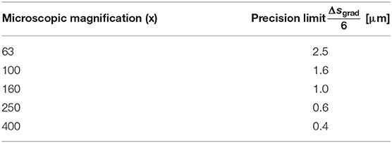
Table 2. Precision limits of microscopic size measurements are derived from the distance between two graduation marks of the ocular micrometer used, and therefore dependent on the microscopic magnification.

2.5. Derivation of Continuous Size Spectra

We applied a Kernel Density Estimation method (e.g., Silverman, 1986) for the derivation of continuous size spectra from discrete microscopic measurements. A Kernel Density Estimate (KDE) was derived for each of the 100 resample datasets. Final size spectra were calculated as means of the ensembles' KDEs together with their respective 95% confidence intervals.

As a first step, the cell volumes were determined based on simple geometric shapes (Edler, 1979; Olenina et al., 2006) and the Equivalent Spherical Diameters (ESD) were calculated. Phytoplankton and protozooplankton have a wide range of geometric shapes, so the volume-dependent ESD was used as a normalized size proxy rather than the length or width dimension of a cell. The length dimension can span from 1 μm in small Micromonas to 1,000μm in long Rhizosolenia cells. In terms of ESD, the range still covers cells from 1 μm–200 μm. The ESD values were log-transformed and normalized by 1 μm:

$\begin{array}{ll}S={\text{log}}_{10}\left(\frac{ESD}{1\text{μm}}\right)& (1)\end{array}$

A KDE is the normalized sum of individual kernels that are themselves probability density functions (pdfs) centered around every data point S_i. The width of the kernels is determined by the bandwidth h (also referred to as smoothing parameter). As a kernel, we applied a Gaussian function, which means that S_i is equal to the first moment (mean) and the bandwidth h is similar to the second moment (standard deviation; see following paragraphs for the selection of h) of a normal probability density function. When a KDE is not normalized with respect to the total number of cells $C_j^{\text{tot}}$ (total number of kernels), it readily represents a plankton size spectrum:

$\begin{array}{ll}KD{E}_j(s,h_j)={\frac{1}{h}}_j{\displaystyle \sum _{i=1}^{C_j^{\text{tot}}}}\frac{1}{\sqrt{2\pi }}\text{exp}\left[-\frac{1}{2}{\left(\frac{s-S_i}{h_j}\right)}^2\right]& (2)\end{array}$

with j being an index of selected data (e.g., split up according to individual taxa or grouped by trophic strategy). The enumerator in the exponent (s−S_i) describes the distance from data point S_i. Since the KDEs have not been normalized we note that they do not represent pdfs, but the following is applicable:

$\begin{array}{ll}\frac{1}{C_j^{\text{tot}}}\times {\displaystyle {\int }_{{\text{log}}_{10}(0.5)}^{{\text{log}}_{10}(500)}}\text{KD}{\text{E}}_j(s,h_j)ds\approx {\displaystyle {\int }_{{\text{log}}_{10}(0.5)}^{{\text{log}}_{10}(500)}}pd{f}_j(s)ds=1& (3)\end{array}$

From the ensemble (KDEs of the 100 resample-datasets), we calculated a mean KDE_j and its standard error (SE). The confidence interval is the mean ${\overline{\text{KDE}}}_j(s)\pm 1.96\times \text{S}{\text{E}}_j(s)$. Despite small confidence intervals, we assume high uncertainty in the cell concentration density estimates for ESDs smaller than ≈ 2 μm that arises out of the limitations in light microscopy (see Table 2). We indicated this uncertainty as dotted lines in the following size spectra.

As described previously, j is an index of selected data. When j is a combined subset of all phytoplankton cells or all zooplankton cells (per sample), the combined size spectrum for all phytoplankton or zooplankton in a dataset is the average of the sample-specific size spectra of phyto- and zooplankton:

$\begin{array}{ll}\text{KD}{\text{E}}_{\text{phy}/\text{zoo}}^{\text{combined}}(s)=\overline{\text{KDE}}(s,h_{\text{phy}/\text{zoo}})& (4)\end{array}$

The bandwidth parameter h controls the degree of smoothing. As described in Schartau et al. (2010), we used a simple rule-of-thumb approach proposed by Silverman (1986). In this plug-in method, an optimal h is estimated from a measure of spread inherent in s, expressed as the standard deviation σ. Since σ is sensitive to outliers, the interquartile range (s_[0.75n] − s_[0.25n]) can serve as a more robust estimator of spread. The optimal estimation for h is:

$\begin{array}{ll}{\widehat{h}}_{opt}=1.06\text{ min}\left\{\sigma ,\frac{s_{\left[0.75n\right]}-s_{\left[0.25n\right]}}{1.34}\right\}{n}^{-\frac{1}{5}}& (5)\end{array}$

The number of selected data subsets (indexed j) can be increased to the total number of taxonomic groups resolved by the microscopic measurements, which allows us to construct composite size spectra with a maximum in resolution. Doing so we learned that the apparent gain in resolution impaired an ascertaining of predominant structural changes, because many additional details were associated with considerable uncertainties. For this reason we resorted to simpler subsets, distinguishing between autotrophic and heterotrophic cells and separating according to sampling periods and locations. Examples of high resolution composite size spectra of phyto- and microzooplankton are provided in the Supplementary Material. We note that the taxonomic precision affects details resolved in composite spectra, because bandwidths ($\widehat{h}$_opt, Equation 5) are then obtained for taxonomic groups individually. In contrast, the combined spectra do not depend on taxonomic precision other than the separation between photoautotrophs and heterotrophs.

2.6. Spatial and Temporal Separation of Observational Data

The Fram Strait's throughflow is characterized by the cold EGC flowing southward, and the warmer WSC flowing northward. In between is a frontal zone of pronounced spatial variability. Some sampling sites were differently affected by one or the other of the two currents. At dates of sampling, these sites were thus subject to a plankton signal that originated either from northern parts of the Fram Strait or from the South. At first we analyzed salinity, density and temperature data, as obtained from the CTD sensors attached to the sampling rosette. We identified individual water masses according to Amon et al. (2003), but distinguishing between Polar Water, Intermediate Water, and Atlantic Water turned out to be vague in certain cases. A sole spatial separation between cold (Polar) and warm (Atlantic) seawater seemed less ambiguous, which we approached by analysing sea surface temperature (SST) data.

We used the High Resolution SST dataset provided by NOAA/OAR/ESRL PSL, Boulder, Colorado, USA¹. We determined daily maps that comprise two distinct spatial areas within the region 10°W–12°E and 77°N–81°N, a “warm” cluster and another that embraces seawater of cold SST. The two spatial clusters were derived with the iterative k-means-clustering method of Hartigan and Wong (1979), as implemented in R (version 3.5.2 R Core Team, 2018). Within a cluster the SST values were alike and horizontal variability remained low. Based on the date and geographical location of sampling, we could eventually assign every sample to either the cold or to the warm SST cluster.

For temporal differences we distinguished between summer and autumn data. Samples from PS99, PS107, and PS114 covered periods in summer, and samples from MSM77 were collected during a cruise in autumn. For putting the spatio-temporal distinguished data into the context of general bloom development, we also compiled a time-series of chlorophyll concentrations for the years 2016–2018 between 10°W–12°E and 77°N–81°N. We used daily chlorophyll-a remote sensing estimates [Level-3 Standard Mapped Image (SMI), Global, 4 km, Chlorophyll, Daily composite data from the Visible and Infrared Imager/Radiometer Suite (VIIRS)], provided by NOAA CoastWatch/OceanWatch². The satellite data were assigned to the SST (cold Polar/warm Atlantic) clusters that had been determined before. A moving average was calculated, with a window width of 15 days, weighed by the number of respective observations for each of the two SST clusters. With the constructed chlorophyll-a time series we could trace the initial build-up, maximum, and decay of the phytoplankton bloom for the three sampling years for both spatial clusters, respectively.

3. Results

3.1. Composition and Abundance of Phyto- and Protozooplankton

We grouped organisms into 61 different identifiable groups (species or higher taxonomic levels) with ESDs ranging from 1 to 196 μm (Figure 2). The smallest of the 42 photo-autotrophic cells were Micromonas sp. (ESD ≈ 1 μm), Rhizosolenia spp. were the largest (ESD > 150 μm). Of the 17 heterotrophic species we found small choanoflagellates (ESD ≈ 1 μm), while the largest heterotrophic dinoflagellate had an ESD of 196 μm. The groups of nano- and microflagellates could not be identified further (in average 10.4% of the total cell concentration), and three cell types were not identifiable at all so only size measurements were taken.

FIGURE 2

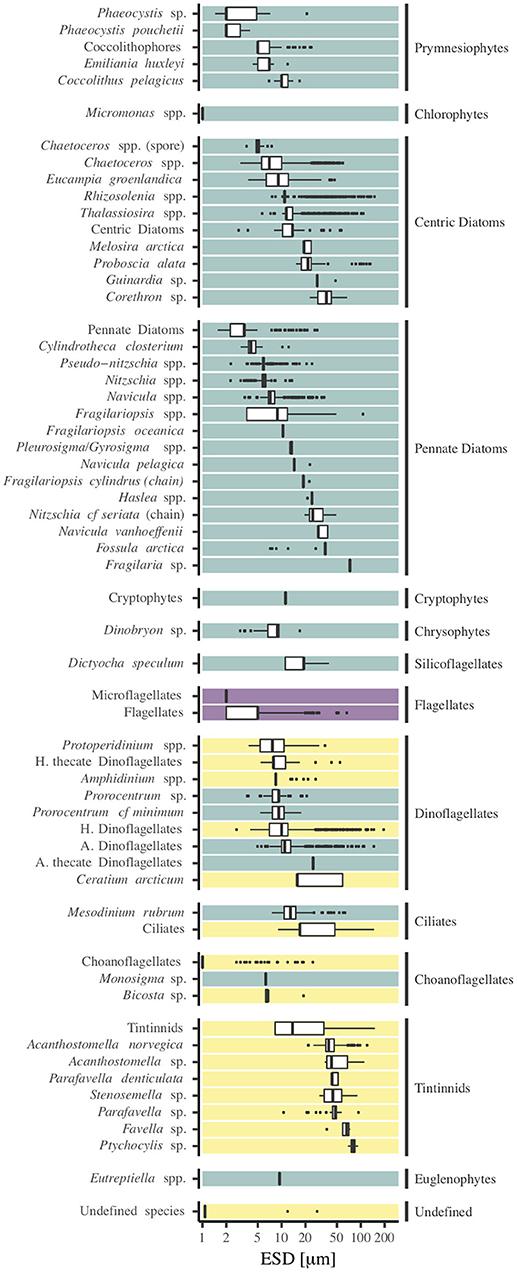
Figure 2. Grouping of all identified species or species groups and their respective size ranges (equivalent spherical diameter (ESD) in μm) on a logarithmic scale. Turquoise species are autotrophic (A.), yellow species are heterotrophic (H.). For purple species, a clear distinction was not possible (in average 10.4% of the total cell concentration), therefore 50% of the cells were treated as autotrophic, and 50% as heterotrophic.

The mean total cell concentration as well as mean total biovolume were generally higher for autotrophic cells (3.02 mm3 L−1; 24.9 × 106 cells L−1) than for heterotrophs, although values differed notably between the cruises (Table 3). The highest cell concentrations were observed in PS107 (44.8 × 106 cells L−1; 5.33 mm3 L−1), followed by PS114 (23.6 × 106 cells L−1; 2.68 mm3 L−1). Phytoplankton concentration was similar in PS99 (3.4 × 106 cells L−1; 0.32 mm3 L−1) and the autumn-cruise MSM77 (4.9 × 106 cells L−1; 1.03 mm3 L−1). Heterotrophic biovolume was 2.30 mm3 L−1 in average, and the mean cell concentration 3.7 × 106 cells L−1, but also varied between the cruises.

TABLE 3

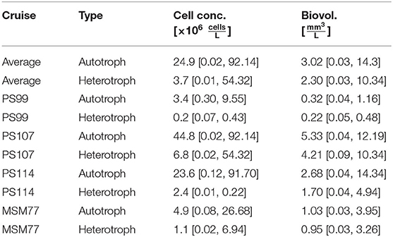
Table 3. Mean [minimum value, maximum value] total cell concentrations and total biovolumes, averaged for all samples and by individual sampling campaigns.

As Figure 2 illustrates, the location of the median cell size varied considerably among species and taxonomic groups. The spread of ESD within species was also highly variable. Variations in cell size were often smaller for precisely identified species than for groups of higher taxonomic level (e.g., flagellates or tintinnids), with exceptions. For most taxa the median ESD laid between 9 and 50 μm.

3.2. Spatial Separation of Cold and Warm Surface Temperature Regimes

With our analyses of SST remote sensing data we were able to separate the water surface of the sampling area (77–81°N, 10°W–12°E) into cold (Polar) and warm (Atlantic) regions for each day of the years 2016–2018. The location of the frontal zone was somewhat variable and changed within days, and we traced how its meandering affected individual sampling sites. Some sites remained within either of the warm or cold clusters at all samplings (e.g., sites EG-1, EG-2, and N-5 within cold; site HG-1 and SV-1 within warm; for a complete list of all stations; see Supplementary Table 1). Especially the central stations, for example sites HG-4 and HG-6, were either subject to cold or to warm waters, depending on the time of sampling. Therefore, the separation was helpful when unraveling differences between the size spectra. An illustration of the variable location of the front relative to the sampling stations is given in Figure 3, displaying four situations during PS99 (Figure 3A), PS107 (Figure 3B), PS114 (Figure 3C), and MSM77 (Figure 3D). Mean SST increased in both regions over the course of the year, reaching their maxima in July (Atlantic section in 2016) or August (Polar section in 2016, both sections in 2017–2018). In the Atlantic region, maximum mean temperatures were between 5.85°C in 2018 and 6.99°C in 2016, whereas the minimum mean temperature was reached between February and April (1.70°C in 2016 and 0.86°C in 2018). The maximum mean temperature in the Polar region was between 0.81°C in 2016 and 1.65°C in 2017. The coldest mean temperature was observed in January 2016 (−1.22°C), and April 2017+2018 (−1.40°C). In the defined area, the Polar region always was in the North-West and the Atlantic in the South-East.

FIGURE 3

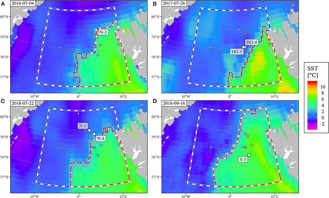
Figure 3. Distinction of Polar (cold, blue dashed line) and Atlantic (warm, red) sections of the study site during the four sampling campaigns. The four snapshots [2016-07-04, PS99 (A), 2017-07-28, PS107 (B), 2018-07-22, PS114 (C), 2018-09-06, MSM77 (D)] illustrate the horizontal variability of the front system. Labeled white squares mark stations sampled on the respective days, remaining stations are indicated as white dots.

Mean total cell concentrations were slightly higher in Polar water samples for both, autotrophs and heterotrophs (26.4 [0.02, 92.14] × 106 cells L−1 and 4.0 [0.01, 54.32] × 106 cells L−1), than in Atlantic water samples (22.1 [0.08, 91.70] × 106 cells L−1 and 3.1 [0.03, 9.22] × 106 cells L−1). While also autotrophic mean total biovolume was higher in Polar samples (3.17 [0.03, 12.19] mm3 L−1 vs. 2.73 [0.03, 14.34] mm3 L−1 in Atlantic samples), heterotrophic biovolume was similar (2.30 [0.04, 9.30] and 2.32 [0.03, 10.34] mm3 L−1). While in the Polar waters autotrophic total biovolume exceeded the heterotrophic total biovolume, similar biovolumes of autotrophs and heterotrophs may indicate a higher activity of the microbial loop in the Atlantic waters.

The size spectra for autotrophs and heterotrophs, separating between Atlantic and Polar samples in Figure 4A, show clear deviations in certain size ranges, in spite of total abundance being similar. Deviations are more pronounced in Figure 4B, where we show the relative difference of the Atlantic (left) and Polar (right) size spectra to the reference (combined-spectra from all samples, see Supplementary Material). Autotrophic cell abundance between 10 and 25 μm (size range D) was higher in the Polar spectrum, as diatoms and chrysophyceans in this size range were more abundant than in Atlantic samples. The high abundance of silicoflagellates and undefined cells around ESD = 40 μm caused an elevated cell concentration density in the Atlantic spectrum relative to the Polar. Large diatoms and autotrophic dinoflagellates around ESD = 110 μm contributed to a local peak, which was missing in the Polar spectrum. Differences between Atlantic and Polar spectra were more noticeable for heterotrophic plankton. Despite high uncertainty, the abundance of cells with ESD < 2 μm was considerably smaller in the Atlantic subset compared to the Polar subset, where small (1 μm) choanoflagellates were common. Interestingly, ciliates in this size range were only observed in Polar samples. However, a high abundance of choanoflagellates, with an ESD around 3 μm, in Atlantic samples lead to a local peak in the Atlantic spectrum in size range A, which was supplemented by ciliates. Since both groups were considerably less abundant in Polar samples, a local minimum could be identified in the size spectrum. The cell concentration density minimum in size range E of the Atlantic spectrum could be attributed to dinoflagellates and flagellates being less abundant relative to the Polar spectrum. The cell concentration density distribution was shifted toward larger ESDs in Atlantic samples, and as a result the Atlantic spectrum exceeded the Polar samples for ESD > 80 μm.

FIGURE 4

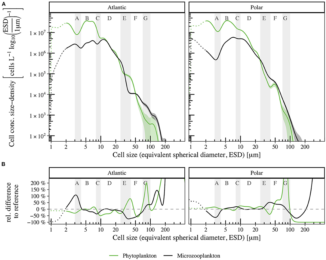
Figure 4. Size spectra for autotrophic phyto- (green) and heterotrophic microzooplankton (black) in samples from the Atlantic (left) and Polar (right) section of the study site (A). Shaded areas indicate the confidence interval (95% CI), dotted lines indicate reduced reliability of size measurements for cells with ESD < 2 μm. Relative differences between the Polar and Atlantic size spectra to the reference (combined spectrum of all samples, see Supplementary Material) in percent (B).

3.3. Spatio-Temporal Distinction of Community Size Spectra

As Figure 5 shows, chlorophyll-a concentration derived through satellite imagery differed over time in the three observed years (temporally) and in the two regions (spatially). From these results we conclude that the development and progression of phytoplankton blooms in the Atlantic and Polar regions of the study site were different. During the four sampling campaigns, protist plankton communities were therefore observed in different growth phases.

FIGURE 5

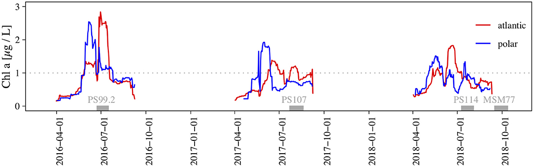
Figure 5. Time series of satellite derived chlorophyll-a concentration estimates. The distinction of Polar and Atlantic areas is described in the materials and methods section. We used daily chlorophyll-a estimates and applied a 15 d moving average, weighed by the number of available data points. Gray bars indicate the duration of sampling campaigns and the dotted gray line indicates the threshold chlorophyll concentration we imposed for classifying as a “bloom” (Wu et al., 2007; Nöthig et al., 2015).

The algal blooms were more intense in the Polar region than the corresponding blooms in the Atlantic region, and started earlier in 2017 and 2018. In the Atlantic region, we observed two pronounced and distinct blooms, with a denser second bloom (2016+2018). The second bloom in the Polar region was hardly expressed. PS99 captured the second bloom of the season in both regions, but while PS107 catched the end of the second bloom in the Atlantic region, the bloom ended already 6 weeks earlier in the Polar region. Chlorophyll-a concentration showed a narrow peak among otherwise moderate values in the Polar region during PS114, and a bloom in the Atlantic region has recently faded. Because of the Polar Night, no satellite observations were available for the autumn cruise MSM77, but in-situ HPLC measurements (data not shown) indicated no further bloom in 2018. A remarkable feature was the increase in variability in autumn. As total cell numbers declined we found certain size ranges with vastly reduced cell numbers (amplified reduction). Size spectra of autotrophs differed greatly in terms of abundance of cells with an ESD < 2 μm. The small chlorophyte Micromonas sp. (ESD ≈ 1 μm) was abundant in summer, but not in autumn. Furthermore, diatoms and the prymnesiophyte Phaeocystis spp., in the size range between 2 and 7 μm, were highly abundant in summer.

By further dividing summer and autumn samples into Polar and Atlantic samples, we could account for spatio-temporal changes in size spectra for autotrophic and heterotrophic plankton (Figure 6). Mean total biovolume was larger in the Atlantic region both in summer and in autumn (Table 4). Furthermore, more autotrophic than heterotrophic biovolume was observed within the investigated size range. In the Polar region, the ratio of autotrophic to heterotrophic biovolume was higher (in summer and autumn) than in the Atlantic region. Autotrophic cell concentration was higher in Atlantic than in Polar samples in summer, and reversed for heterotrophs. In autumn, both autotrophic and heterotrophic cell concentrations were higher in the Atlantic region than in the Polar region.

FIGURE 6

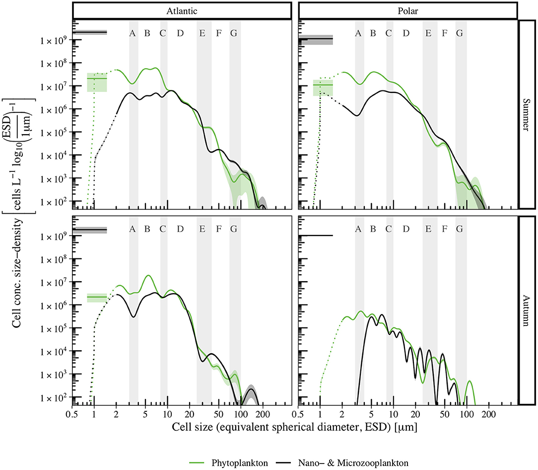
Figure 6. Abundance size spectra for phyto- (green) and microzooplankton (black) of temporally (summer, top panels; autumn, bottom panels) and spatially (Atlantic, left panels; Polar, right panels) separated data. Colored shaded areas indicate the 95% confidence intervals, dotted lines indicate reduced reliability of size measurements for cells with ESD < 2 μm. For comparison, cell concentration densities derived from Flow Cytometry measurements are shown for bacteria (black line, 0.5–1.5 μm, data from corresponding samples in von Jackowski et al. (2020) and for Synechococcus (green line, 0.8–1.5 μm, data from Paulsen et al., 2016; August-south $\stackrel{\wedge }{=}$ Summer-Atlantic, August-north $\stackrel{\wedge }{=}$ Summer-Polar, November $\stackrel{\wedge }{=}$ Autumn-Atlantic).

TABLE 4

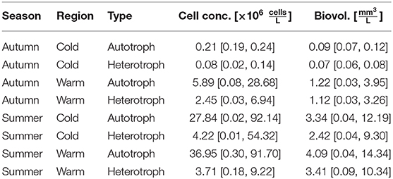
Table 4. Average and [minimum value, maximum value] total cell concentrations and total biovolumes for a spatio-temporally separated dataset.

As Figure 6 (upper panels) shows, Atlantic (left) and Polar (right) size spectra aligned relatively well in summer. However, autotrophic cell concentration density for Atlantic samples was slightly elevated in section B, because even though less diatoms were observed, substantially more prymnesiophytes of this size range were found compared to Polar samples. Mismatches in sections E and > G related to higher dinoflagellate and diatom concentrations in Atlantic samples. Differences in the size distribution of choanoflagellates caused the contrary course of Polar and Atlantic heterotrophic size spectra. Furthermore, less flagellates and dinoflagellates in section E caused a local minimum in the Atlantic spectrum around 40 μm.

In autumn (Figure 6, lower panels), differences between Polar and Atlantic spectra were considerably more pronounced. Autotrophic and heterotrophic cell concentration densities were smaller for ESD < 30 μm, and converged for larger cells. No chlorophytes were observed in autumn, and the cell concentration density of small prymnesiophytes and diatoms was lower in the Polar than in the Atlantic spectrum. In sections A–D, the autotrophic spectra ran relatively parallel, with reduced cell concentration densities in the Polar spectrum (less diatoms and dinoflagellates), and then converged. In contrast to smaller size ranges, diatoms with ESD ≈ 120 μm were more common in the Polar samples. While the Atlantic size spectrum for heterotrophic cells in autumn covered a size range of 1–180 μm, the Polar spectrum only covered 3–80 μm.

The Atlantic and Polar biovolume size spectra shown in Figure 7 likewise showed less deviation in summer, compared to autumn. In the size ranges 3–4 and 8–10 μm the biovolume size density was consistently reduced relative to its neighboring size ranges in all spatio-temporally separated spectra. Furthermore, the size ranges 35–40 and 70–100 μm frequently contained local minima and generally expressed high variability.

FIGURE 7

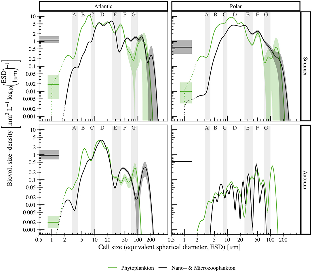
Figure 7. Biovolume size spectra for phyto- (green) and microzooplankton (black) of temporally (summer, top panels; autumn, bottom panels) and spatially (Atlantic, left panels; Polar, right panels) separated data. Colored shaded areas indicate the 95% confidence intervals, dotted lines indicate reduced reliability of size measurements for cells with ESD < 2 μm. For comparison, biovolume concentration densities derived from Flow Cytometry cell count measurements are shown for bacteria (black line, 0.5–1.5 μm, assuming mean ESD = 1 μm, data from corresponding samples in von Jackowski et al. (2020) and for Synechococcus (green line, 0.8–1.5 μm, assuming mean ESD = 1.2 μm, data from Paulsen et al., 2016).

4. Discussion

4.1. Changes in Plankton Community Structure in the Arctic

A long-term gradual increase in phytoplankton biomass was reported for the West Spitsbergen Current (WSC) in the Fram Strait by Nöthig et al. (2015). According to an analysis of satellite-derived chlorophyll-a data of the period between 1991 and 2012, this temporal trend is evident for the warmer Atlantic waters entering the Arctic ocean through the Fram Strait but not for the southward moving colder Polar waters (Nöthig et al., 2020). Following a warm water anomaly between the years 2005 and 2007, Nöthig et al. (2015) also observed a shift in species composition, from a domination of diatoms toward smaller sized cells of haptophyte Phaeocystis and other nanoflagellates in the Atlantic waters of the WSC during the summer months. Our data from 2016, 2017, and 2018 include measurements of Phaeocystis, whose abundance and biovolume decreased from summer to autumn. In both seasons, abundance and biovolume were always higher in Atlantic than in Polar waters.

Changes in plankton composition in the Arctic also involve shifts in the abundance of picophytoplankton, like Micromonas and Synechococcus. Significantly high cell numbers of picophytoplankton were found within the WSC northwest of Spitsbergen, of Synechococcus (Paulsen et al., 2016) as well as of Micromonas (Kilias et al., 2014). The presence of autotrophic picoplankton in northern polar regions was emphasized by Li et al. (2009), who discovered an increase in the abundance of small picoplankton (< 2 μm) in the Canada Basin between 2004 and 2008. This finding was linked to a freshening of surface waters. Likewise, Comeau et al. (2011) stressed the tendency toward observing higher abundance of small plankton cells like haptophytes and Micromonas in the Canadian Beaufort region, which they attributed to enhanced stratification and thus general decrease in nitrate availability. Paulsen et al. (2016) highlighted the high abundance of Synechococcus in August 2014, which was similar to the abundance of Micromonas resolved by our summer microscopic data from the years 2016, 2017, and 2018. In October Micromonas was nearly absent, while significant numbers of Synechococcus can be found even in November within the Atlantic water (Paulsen et al., 2016). On the one hand, the biovolume of Synechococcus reported for November 2014 in Paulsen et al. (2016) is a small fraction relative to our total biovolume estimates of October (see Figures 6, 7). On the other hand, the abundance of Synechococcus might have been higher during October in that year than in November. Paulsen et al. (2016) explained the presence of Synechococcus could be associated with a reduced grazing pressure by heterotrophic nanoflagellates. Our spectra support their interpretation, as we could reveal a drastic decline in heterotrophic nanoflagellate abundance (between 3 and 4 μm) already in the Polar water's summer spectrum and even more so in the autumn spectrum of the Atlantic water (Figures 6, 7). In the Polar water we did not find a significant number of heterotrophic nanoflagellates in October. We here recall the differences between the Polar- and Atlantic water with respect to the timing of the bloom and the successional plankton development, as shown in Figure 5. This indicates that the plankton signal in the Atlantic water was lagged by several weeks compared to the Polar water, and Synechococcus might have been present at higher abundance in October in the Polar water as well, which remained unresolved in our measurements.

Overall, recent observations substantiate the appearance of autotrophic picoplankton in the Arctic, with potential consequences for the functioning of the microbial loop dynamics. However, we learned that great care has to be taken when making inferences about a general trend with respect to heterotrophic bacteria and autotrophic picoplankton in a changing Arctic. Given the high variability in the abundance of the picoplankton it remains difficult to assess whether shifts toward higher abundance of smaller cells can be attributed to variations in timing of the seasonal succession or is a general phenomenon. In this context, it becomes meaningful to relate the here observed spectra to the seasonal bloom development, which will be further addressed in section 4.3.

4.2. Specific Patterns in Plankton Size Spectra

Based on our size spectra we identified distinctive size ranges of local maxima and minima. Four size ranges of high variability at 3–4, 8–10, 25–40, and 70–100 μm indicate size-selective grazing. These patterns cannot be explained by allometric physiological processes of the phytoplankton, because they appeared in size spectra for both, autotrophic and heterotrophic cells. Rather, the variability within these specific size intervals accentuate variations between bottom-up effects and top-down control through grazing. Furthermore, the distinctive size ranges denote the importance of prey size, with no clear discrimination according to the trophic status (omnivory). In contrast, interjacent size ranges showed noticeably less variability, suggesting that these size ranges were less influenced by variations in grazing. Similar size specific patterns had been observed in other studies. For example, Schartau et al. (2010) used a similar approach to generate size-spectra from epi-fluorescence microscopic plankton counts and size measurements from equatorial Pacific samples (Landry et al., 2000). They observed a clear minimum around 4 μm ESD, and a step-like decrease between 30 and 50 μm ESD, which became even more pronounced in samples of a fertilized patch where algal growth was stimulated by the addition of iron. The depression in the proximity of 4 μm ESD of the plankton community size structure was so prominent that it could readily be identified by histogram representations of fixed size classes, with lowered cell abundance in the 2–5 μm size class of the original data set described in Landry et al. (2000). Mainly heterotrophic flagellates, dinoflagellates, prymnesiophytes, and small diatoms were subject to this size-specific grazing impact. Rodríguez et al. (1998) compiled size-abundance spectra for samples from the deep fluorescence maxima at different locations in the Alboran Sea (Mediterranean), combining flow cytometry and microscopy data. Consistently, the abundance of cells between 5 and 6 μm ESD was reduced relative to smaller and larger cells. In a size spectrum compiled by Marañón (2015), log(cell abundance) deviates notably from the linearly decreasing relationship with log(cell volume), especially in a cell size range around 4 μm. Similarly, in size spectra derived by Quinones et al. (2003) from image analyses of samples from the North-West Atlantic, anomalies in biovolume (deviations from a log-linear relationship) are traceable at sizes 3–4 μm and at approximately 30–40 μm. Volume size spectra derived from Laser in-situ Scattering and Transmissometry (LISST) measurements in the Fram Strait by Trudnowska et al. (2018) show maxima in phytoplankton biovolume between 4 and 5 μm, with much lower values for sizes greater than 10 μm. Their spectral measurements represent conditions found in the middle of July 2013. In contrast to their LISST data, our spectra exhibit a substantial fraction of phytoplankton biovolume also in the size range >10 μm not only in summer but also in autumn. Interestingly, the total particle spectra (of the phyto- and other- types of particles) resolved by LISST in Trudnowska et al. (2018) disclose minima between 20 and 30 μm, most noticeably for measurements in the WSC.

Moreno-Ostos et al. (2015) derived a series of size abundance spectra from samples collected in the subtropical Atlantic (south and north of the equator). They concluded that the spectral slope of a log-linear size-abundance relationship of the phytoplankton is not a good indicator for total biovolume, in particular within oligotrophic waters. This was attributed to considerable variability within specific size ranges so that slope and intercept may not become ultimately constrained by the size and abundance data. Amongst size ranges of large variations in their study were those in the vicinity of 4 μm (volume ≈ 101.5 μm3), as well as between 27 μm and 50 μm (volume ranges of ≈ 10⁴–104.8 μm3). Clearly, some of the prominent size ranges with pronounced variations revealed in our study for the Arctic microbial plankton community seem to be generic rather than site-specific.

4.3. Spatial and Temporal Separation

In the study of Trudnowska et al. (2016), spatial variability in the Fram Strait was investigated in July 2012. They could resolve patches of high plankton abundance that occupied between 2 and 17 % of the Fram Strait region. According to their analysis, major differences in normalized biovolume size-spectra could be mainly attributed to differences in oceanographic conditions. For example, consistent with our observations, phytoplankton in the WSC region were larger (higher abundance in the size range larger than 100 μm) than in the Polar water. Based on our analyses of remote sensing chlorophyll-a concentrations, we showed that the temporal development of chlorophyll-a differed between the Polar and Atlantic water masses. The spring blooms in Polar waters appeared earlier than the pronounced blooms of the Atlantic waters, which is consistent with the results of Nöthig et al. (2015), who revealed differences in the variability, trends and bloom duration between EGC and WSC in the period 1991–2012.

Because our samples covered the Polar and Atlantic water masses as well as two different seasons (summer and autumn), we may interpret the spatio-temporally separated size spectra (section 3.3) as independent size spectra that represent four different points in time, relative to the progression of the plankton community succession: Scenario 1–4 (S1–S4, approximately 0, 1–8, 9–11, and 15–17 weeks after the bloom maximum, Figure 8). During the summer cruises (PS99, PS107, PS114), remote sensing indicated high chlorophyll-a averages in the Atlantic section of the sampling site. We therefore interpret size spectra from Atlantic summer samples as Scenario 1 (S1), as they originate from mid to end of bloom situations. Mean chlorophyll-a concentration had decreased already in the Polar section during the summer cruises, and the peak bloom had passed approximately 1–8 weeks ago (S2). In 2018, chlorophyll-a concentration in the Atlantic section peaked approximately 9–11 weeks before MSM77-sampling was undertaken, hence we interpret Atlantic autumn spectra as S3. Mean chlorophyll-a concentration peaked earlier, throughout May in 2018, in the Polar section, so 15–17 weeks passed between the end of the bloom in early June until sampling during MSM77. Polar autumn size spectra therefore represent S4.

FIGURE 8

Figure 8. Spectra at different times relative to the progression of plankton succession (S1–S4). During the summer cruises, the Atlantic waters were subject to bloom conditions (S1 ≈ 0 weeks after bloom), while in the Polar waters the peak bloom had already passed (S2 ≈ 1–8 weeks after bloom). The spatio-temporal separation of the autumn spectra was done likewise (S3 ≈ 9–11, and S4 ≈ 15–17 weeks after bloom). Abundance spectra are shown in (A), biovolume spectra in (B). Dotted lines indicate reduced reliability of size measurements for cells with ESD < 2 μm. For comparison, abundance and biovolume concentration densities derived from Flow Cytometry cell count measurements are shown for bacteria as horizontal lines (0.5–1.5 μm, assuming mean ESD = 1 μm, data from corresponding samples in von Jackowski et al. (2020).

With this approach we could resolve changes in plankton size structure, revealing that while mean total cell concentration and total biovolume decreased (see Supplementary Figure 3), major patterns strengthened, diminished, or even reversed. For example, the maximum around 3 μm in the heterotrophic spectrum at S1 turned to a local minimum at S3–S4. During the decline of the phytoplankton community, the relative abundance of smaller sized cells (ESD < 30 μm) decreased more than the number of larger cells. If interpreted in terms of a log-linear relationship between abundance and ESD, this corresponds to a reduction of the slope. The gradual reduction of the abundance of small cells eventually induced a sign-change in the slope of phytoplankton biovolume spectrum (see Figure 8B), with the biovolume being dominated by cells of ESD > 10 μm. During S4, the maximum abundance of autotrophs was at ESD ≈ 3 μm, which is a size range of noticeable grazing pressure, appearing as a local trough at other times. This inversion suggests some potential for recovery of the standing stocks in this size range. Interestingly, Marañón et al. (2013) showed experimentally that the size-dependent maximum growth rate μ_max has an optimum in the vicinity of this size range, likely as a result of a trade-off between the ability to replenish internal nutrient cell quota and the ability to synthesize new biomass (Ward et al., 2017).

According to our spectra, the size-selective grazing showed clear signs of omnivory, but also of intraguild predation within the microbial community. Ciliates are often regarded as a single functional group (guild) in models of the microbial loop (e.g., Thingstad and Cuevas, 2010). Stoecker and Evans (1985) have shown experimentally that while both, the large tintinnid Favella sp. and the smaller ciliate Balanion sp. fed on the dinoflagellate Heterocapsa triquetra, the large tintinnid could also prey on the smaller ciliate. In their model, ecosystem structure was shaped by the relative efficiencies of the one-step and the two-step pathway of this triangular trophic relationship. The results of our analysis agree with their findings. In our spectra the ciliates occupied a broad size range, from 7 μm small undefined ciliates to the tintinnid Acanthostomella norvegica with ESD = 120 μm, while the majority of cliliates were larger than 10 μm. Heterotrophic cells in the 25–40 μm size range (section E) were composed mainly from dinoflagellates, tintinnids, and other ciliates in slightly varying proportions between S1 and S3, but the absence of ciliates and tintinnids < 40 μm caused a prominent trough at S4. The density of larger tintinnids between 35 and 90 μm however stayed relatively constant, which could indicate a transition from mainly herbivory on phytoplankton to increasing carnivory on smaller ciliates, their former competitors, as total phytoplankton declines. The consideration of larger ciliates grazing on smaller ones increases the length of the food chain and thus the number of loops, which could be approached by considering the theory and size-based model of multiple food chains suggested by Armstrong (1994). For every additional loop cycle within the microbial food web the efficiency of matter transfer to the copepods is reduced, while more organic matter is released and becomes available for bacterial consumption (Azam et al., 1983), with potential consequences for nutrient recycling and organic matter export (Steele, 1998). Although unresolved by our spectra, the loss of the largest microzooplankton (tintinnids and heterotrophic dinoflagellates > 80 μm) at S4 and the decrease of large diatoms were likely associated with copepod grazing and aggregation.

4.4. ESD and Effective Prey Size of Plankton

When comparing plankton size spectra, certain aspects of how cell size was measured and normalized have to be considered. For unicellular nano- and microplankton we could demonstrate that the ESD can be a robust measure of size, otherwise our spectra would have become more blurred because of the various cell shapes and thus distinct patterns would not have been identifiable. Our ESD values are based on cell volumes that were derived from length and width measurements, thereby considering differences in the plankton cell's geometric shapes described in Edler (1979) and Olenina et al. (2006). This approach is more advanced than assuming ellipsoids, but with respect to biovolume, the ESD is likely a less accurate proxy than the area-based diameter (ABD), a normalized measure based on the entire area of a single cell or organism of various shapes. The ABD is a valuable approximation of the biovolume, which would be a good measure for investigating allometric physiological dependencies, e.g., size dependent variations in nutrient affinity (e.g., Aksnes and Egge, 1991). In our plankton size spectra we could identify recurrent patterns but did not find a perfect match in ESD of the distinctive minima due to size-selective grazing. This is likely because of morphological differences. The ESD of a prey cell does not necessarily reflect the actual dimension that a predator might face. For example, the star-shaped Dictyocha speculum has a relatively small cell volume and a small ESD accordingly, but appears bulky due to its spines. Care has to be taken when elaborating predator-prey interactions from changes in ESD based size spectra. In other words, while ESD might work well for explaining bottom-up allometric effects we do not expect that ESD is equally representative as prey size. Identical ESDs can be assigned to cells of very different morphology. Bearing this in mind, we recommend the consideration of an effective prey size when looking at predator-prey dependencies, while using ESD for biovolume dependent processes. In this manner, the formation of colonies impacts the effective prey size, with ecological implications.

We treated cells that were part of colonies as single cells, because the sample fixation with hexamine neutralized formaldehyde may have an impact on the durability of cell colonies. The prymenesiophyte Phaeocystis sp. can reach high abundance in the Marginal Ice Zone (Gradinger and Baumann, 1991; Nöthig et al., 2015) and is known to occur in form of small flagellated cells or to grow to large colonies (Rousseau et al., 2007). We observed mostly free living, flagellate single cells of P. pouchetii with an average diameter of 2.4 μm, while spherical colonies can reach 0.1 mm and cloud-shaped colonies may reach 2 mm, as reviewed in Rousseau et al. (2007). Interestingly, with the formation of colonies, the P. pouchetii cells can overrun the 8–10 and 25–40 μm size ranges of definite grazing pressure, generating a loophole for their growth and reaching the size range of large chain forming diatoms. Such an effect could not be resolved with our measurements, but should be better addressed in future studies. The formation of colonies is hypothesized to be a defence mechanism against microzooplankton grazers, with the consequence of entering the size range of prey for copepods (Nejstgaard et al., 2007). Furthermore, some diatom species are known to form chains to escape size ranges of high grazing pressure (Bjærke et al., 2015). In our study we indeed observed colonial assemblages of Chaetoceros sp., Pseudo-nitzschia spp., Eucampia groenlandica, Navicula vanhoeffenii, Navicula pelagica, Navicula sp., Fragilariopsis spp., Fossula arctica, and other undefined pennate diatoms.

4.5. Limitations and Outlook

Microscopic measurements depend on the experience of the observer. Therefore, comparisons between data or their combination need to made with caution. We respected uncertainties in plankton counts and in size measurements by introducing a resampling approach, but some uncertainties in taxonomic identification may still exist. A study by Jakobsen et al. (2015) has shown large variations not only between different taxonomists, but also for repeated measurements of the same taxonomists. The purpose of grouping and averaging size-spectra of individual samples was to eliminate potential biases and compensate for major methodological variations. The mixotrophic lifestyle may be common or even predominant among protist plankton (Flynn et al., 2013), however we could not resolve this microscopically. Instead, all dinoflagellates containing chloroplasts were regarded as photo-autotrophic, and the colorless as heterotrophic. We furthermore assigned half of the flagellates an autotrophic and half a heterotrophic nutrition, which contributes to further blur in the trophic identifications. Our classifications of autotrophic and heterotrophic feeding modes therefore do not refer to strict trophic strategies, but rather indicate a tendency toward one or the other, without resolving all intermediate lifestyles.

All samples considered in our analysis were collected during four cruises within a three years period, covering different times of the natural plankton succession in the Fram Strait. Each of the cruises span a 3 week period, being “snapshots” of the protist plankton community. In spite of these short term observations, the specific size ranges discussed above were distinctive within all size spectra, which implies that the trophic dynamics of the microbial community in the Fram Strait are well reflected in our size spectra within the size range between 2 and 200 μm. Considerable uncertainties exist in our spectra for sizes smaller than 2 μm. With our microscopic measurements we could not resolve the abundance of picoplanktonic cyanobacteria and of heterotrophic bacteria. However, for comparison we considered picoplankton data from the studies of von Jackowski et al. (2020) (bacteria) and Paulsen et al. (2016) (Synechococcus). These data are typically available as measurements of a different type, e.g., flow cytometry. Likewise, the consideration of copepod data would provide a more complete picture of the microbial loop dynamics, including mass transfer. A synthesis of our derived size spectra with complementary ecological and biochemical data appears as constructive objective for future studies.

The here presented size spectra are particularly valuable for constraining solutions obtained by size-based model applications. Only by modeling we could disentangle some of the complex interdependencies between the phyto- and the microzooplankton. Our spectra reflect the state of the microbial community structure at times after the bloom maximum, a period when the microbial dynamics is critical for regenerated production. The identified size ranges of high grazing pressure and size niches that favor autotrophic growth impose strong constraints on model solutions, in particular with respect to resolving variations between bottom-up and top-down regulatory effects and trophic efficiency. The latter is of vital importance for estimating mass transfer to higher trophic levels in model applications, i.e., prey availability for copepods.

5. Conclusion

The primary aim of our study was to gain insight to the plankton community size structure within the Arctic environment of the Fram Strait. The employed KDE method for analysing the size structure (as equivalent spherical diameter, ESD) of the nano- and microplankton community was shown to reveal details that may become masked by introducing individual size classes. In conclusion, with our extensive approach we documented how laborious and thus valuable microscopic measurements can be well transferred to continuous size spectra of autotrophic and heterotrophic plankton of ESD between 1 μm and ≈ 200 μm. With this approach we could accentuate details that show distinct deviations from any log-linear dependency between plankton size, abundance, and biovolume.

From our remote sensing data analyses we learned that the plankton community within the polar Arctic Water lead the seasonal succession by approximately 2–3 weeks relative to the plankton observed in the Atlantic Water. Our plankton size spectra document the decline in total biovolume during the post bloom period as well as a substantial shift in the phytoplankton's relative biovolume toward larger cell sizes (> 30 μm) in autumn. We conclude that the spatial separation between Arctic and Atlantic waters within the Fram Strait was crucial, as both water masses contained plankton and likely a biogeochemical signal that differed with respect to the timing in seasonal succession.

Amongst the most interesting details are four specific size ranges (3–4, 8–10, 25–40, 70–100 μm). The four size ranges induce pronounced deviations from a log-linear dependency between plankton size, abundance, and biovolume. Thus, these specific size ranges appear to be valuable indicators for temporal changes between bottom-up and top-down regulatory processes within the microbial food web.

The identified size ranges disclose size-selective grazing impacts on the Arctic nano- and microplankton community, regardless of the trophic status. Since autotrophs and heterotrophs seemed to be subject to similar grazing pressures within specific size ranges, we conclude that the conjecture of phytoplankton and heterotrophic nanoflagellates being the only prey for ciliates is inappropriate. Instead, omnivory and intraguild predation seem to be vital pathways within the pelagic microbial food web in the Arctic. Whether the identified grazing-sensitive size ranges are specific for the Arctic or generic for the microbial food webs remained unresolved here, but comparisons with other spectra clearly indicated similar grazing impacts, at least within the size ranges 3–4 and 25–40 μm.

Data Availability Statement

The data analyzed in this study is subject to the following licenses/restrictions. Results from data analysis (individual size-spectra) will be made available via institutional (GEOMAR) repository. Requests to access these datasets should be directed to Vanessa Lampe, vlampe@geomar.de.

Author Contributions

VL generated and analyzed the size spectra and produced all figures and tables. E-MN provided the microscopic measurements, based on samples collected during four cruises to the Fram Strait. She guided the analysis with respect to discrimination between taxonomic groups and trophic strategies. MS initiated this study and guided the analyses with respect to the statistical methods applied. All authors contributed in writing the manuscript.

Funding

This study was funded by the Helmholtz Association and the German Federal Ministry of Education and Research (BMBF) as a contribution to the microARC project (03F0802A), part of the Changing Arctic Ocean programme, jointly funded by the UKRI Natural Environment Research Council (NERC) and BMBF.

Conflict of Interest

The authors declare that the research was conducted in the absence of any commercial or financial relationships that could be construed as a potential conflict of interest.

Acknowledgments

Data were obtained during four POLARSTERN and MARIA S. MERIAN cruises and we thank the captains and crews. Special gratitude is owed to the student helpers Malte Schmidt and Lisa Zacharski for their tedious hours of plankton counting. We thank Ben Ward, whose comments helped improving the manuscript. Fruitful discussions about the Arctic plankton community with Neil Banas and Friederike Prowe are much appreciated. We are grateful for constructive comments by the two reviewers.

Supplementary Material

The Supplementary Material for this article can be found online at: https://www.frontiersin.org/articles/10.3389/fmars.2020.579880/full#supplementary-material

Footnotes

1. ^https://psl.noaa.gov/data/gridded/data.noaa.oisst.v2.highres.html (accessed February 21, 2019)

2. ^https://coastwatch.noaa.gov/cw/satellite-data-products/ocean-color/science-quality/viirs-snpp.html (accessed July 31, 2019)

References

Acevedo-Trejos, E., Mara nón, E., and Merico, A. (2018). Phytoplankton size diversity and ecosystem function relationships across oceanic regions. Proc. R. Soc. B Biol. Sci. 285:1879. doi: 10.1098/rspb.2018.0621

PubMed Abstract | CrossRef Full Text | Google Scholar

Aksnes, D. L., and Egge, J. K. (1991). A theoretical model for nutrient uptake in phytoplankton. Mar. Ecol. Prog. Ser. 70, 65–72. doi: 10.3354/meps070065

CrossRef Full Text | Google Scholar

Amon, R. M. W., Budéus, G., and Meon, B. (2003). Dissolved organic carbon distribution and origin in the Nordic Seas: exchanges with the Arctic Ocean and the North Atlantic. J. Geophys. Res. 108, 1–17. doi: 10.1029/2002JC001594

CrossRef Full Text | Google Scholar

Armstrong, R. A. (1994). Grazing limitation and nutrient limitation in marine ecosystems: steady state solutions of an ecosystem model with multiple food chains. Limnol. Oceanogr. 39, 597–608. doi: 10.4319/lo.1994.39.3.0597

CrossRef Full Text | Google Scholar

Azam, F., Fenchel, T., Field, J. G., Gray, J. S., Meyer-Reil, L. A., and Thingstad, F. (1983). The ecological role of water-column microbes in the Sea. Mar. Ecol. Prog. Ser. 10, 257–263. doi: 10.3354/meps010257

CrossRef Full Text | Google Scholar

Bakun, A., and Broad, K. (2003). Environmental–loopholes' and fish population dynamics: comparative pattern recognition with focus on El Ni no effects in the Pacific. Fisher. Oceanogr. 12, 458–473. doi: 10.1046/j.1365-2419.2003.00258.x

CrossRef Full Text | Google Scholar

Barton, A. D., Pershing, A. J., Litchman, E., Record, N. R., Edwards, K. F., Finkel, Z. V., et al. (2013). The biogeography of marine plankton traits. Ecol. Lett. 16, 522–534. doi: 10.1111/ele.12063

PubMed Abstract | CrossRef Full Text | Google Scholar

Barton, B. I., Lenn, Y. D., and Lique, C. (2018). Observed atlantification of the Barents Sea causes the Polar Front to limit the expansion of winter sea ice. J. Phys. Oceanogr. 48, 1849–1866. doi: 10.1175/JPO-D-18-0003.1

CrossRef Full Text | Google Scholar

Beszczynska-Möller, A., Fahrbach, E., Schauer, U., and Hansen, E. (2012). Variability in Atlantic water temperature and transport at the entrance to the Arctic Ocean, 1997-2010. ICES J. Mar. Sci. 69, 852–863. doi: 10.1093/icesjms/fss056

CrossRef Full Text | Google Scholar

Bjærke, O., Jonsson, P. R., Alam, A., and Selander, E. (2015). Is chain length in phytoplankton regulated to evade predation? J. Plankton Res. 37, 1110–1119. doi: 10.1093/plankt/fbv076

CrossRef Full Text | Google Scholar

Chisholm, S. W. (1992). “Phytoplankton size,” in Primary Productivity and Biogeochemical Cycles in the Sea, eds P. G. Falkowski, A. D. Woodhead, and K. Vivirito (Boston, MA: Springer Science and Business Media), 213–237. doi: 10.1007/978-1-4899-0762-2_12

CrossRef Full Text | Google Scholar

Comeau, A. M., Li, W. K., Tremblay, J. É., Carmack, E. C., and Lovejoy, C. (2011). Arctic ocean microbial community structure before and after the 2007 record sea ice minimum. PLoS ONE 6:27492. doi: 10.1371/journal.pone.0027492

PubMed Abstract | CrossRef Full Text | Google Scholar

Comiso, J. C., and Hall, D. K. (2014). Climate trends in the Arctic as observed from space. Wiley Interdisc. Rev. 5, 389–409. doi: 10.1002/wcc.277

PubMed Abstract | CrossRef Full Text | Google Scholar

de Steur, L., Hansen, E., Gerdes, R., Karcher, M., Fahrbach, E., and Holfort, J. (2009). Freshwater fluxes in the East Greenland Current: a decade of observations. Geophys. Res. Lett. doi: 10.1029/2009GL041278. [Epub ahead of print].

CrossRef Full Text | Google Scholar

Edler, L. (1979). Recommendations on Methods for Marine Biological Studies in the Baltic Sea: Phytoplankton and Chlorophyll. Publication: Baltic Marine Biologists. Department of Marine Botany, University of Lund.

Google Scholar

Falkowski, P. G., Barber, R. T., and Smetacek, V. (1998). Biogeochemical controls and feedbacks on ocean primary production. Science 281, 200–206. doi: 10.1126/science.281.5374.200

PubMed Abstract | CrossRef Full Text | Google Scholar

Falk-Petersen, S., Haug, T., Hop, H., Nilssen, K. T., and Wold, A. (2009). Transfer of lipids from plankton to blubber of harp and hooded seals off East Greenland. Deep-Sea Res. Part II Top. Stud. Oceanogr. 56, 2080–2086. doi: 10.1016/j.dsr2.2008.11.020

CrossRef Full Text | Google Scholar

Finkel, Z. V., Beardall, J., Flynn, K. J., Quigg, A., Rees, T. A. V., and Raven, J. A. (2010). Phytoplankton in a changing world: Cell size and elemental stoichiometry. J. Plankton Res. 32, 119–137. doi: 10.1093/plankt/fbp098

CrossRef Full Text | Google Scholar

Flynn, K. J., Stoecker, D. K., Mitra, A., Raven, J. A., Glibert, P. M., Hansen, P. J., et al. (2013). Misuse of the phytoplankton-zooplankton dichotomy: the need to assign organisms as mixotrophs within plankton functional types. J. Plankton Res. 35, 3–11. doi: 10.1093/plankt/fbs062

CrossRef Full Text | Google Scholar

Gradinger, R. R., and Baumann, M. E. (1991). Distribution of phytoplankton communities in relation to the large-scale hydrographical regime in the Fram Strait. Mar. Biol. 111, 311–321. doi: 10.1007/BF01319714

CrossRef Full Text | Google Scholar

Hartigan, J. A., and Wong, M. A. (1979). Algorithm AS 136: A K-means clustering algorithm. Appl. Stat. 28, 100–108. doi: 10.2307/2346830

CrossRef Full Text | Google Scholar

Huete-Ortega, M., Cerme no, P., Calvo-Díaz, A., and Mara nón, E. (2012). Isometric size-scaling of metabolic rate and the size abundance distribution of phytoplankton. Proc. R. Soc. B Biol. Sci. 279, 1815–1823. doi: 10.1098/rspb.2011.2257

PubMed Abstract | CrossRef Full Text | Google Scholar

Huete-Ortega, M., Mara nón, E., Varela, M., and Bode, A. (2010). General patterns in the size scaling of phytoplankton abundance in coastal waters during a 10-year time series. J. Plankton Res. 32, 1–14. doi: 10.1093/plankt/fbp104

CrossRef Full Text | Google Scholar

Irigoien, X., Flynn, K. J., and Harris, R. P. (2005). Phytoplankton blooms: a ‘loophole’ in microzooplankton grazing impact? J. Plankton Res. 27, 313–321. doi: 10.1093/plankt/fbi011

CrossRef Full Text | Google Scholar

Jakobsen, H. H., Carstensen, J., Harrison, P. J., and Zingone, A. (2015). Estimating time series phytoplankton carbon biomass: Inter-lab comparison of species identification and comparison of volume-to-carbon scaling ratios. Estuar. Coast. Shelf Sci. 162, 143–150. doi: 10.1016/j.ecss.2015.05.006

CrossRef Full Text | Google Scholar

Kilias, E. S., Nöthig, E. M., Wolf, C., and Metfies, K. (2014). Picoeukaryote plankton composition off West Spitsbergen at the entrance to the Arctic Ocean. J. Eukaryot. Microbiol. 61, 569–579. doi: 10.1111/jeu.12134

PubMed Abstract | CrossRef Full Text | Google Scholar

Landry, M. R., Ondrusek, M. E., Tanner, S. J., Brown, S. L., Constantinou, J., Bidigare, R. R., et al. (2000). Biological response to iron fertilization in the eastern equatorial Pacific (IronEx II). I. Microplankton community abundances and biomass. Mar. Ecol. Prog. Ser. 201, 27–42. doi: 10.3354/meps201027

CrossRef Full Text | Google Scholar

Larsen, A., Egge, J. K., Nejstgaard, J. C., Di Capua, I., Thyrhaug, R., Bratbak, G., et al. (2015). Contrasting response to nutrient manipulation in Arctic mesocosms are reproduced by a minimum microbial food web model. Limnol. Oceanogr. 60, 360–374. doi: 10.1002/lno.10025

PubMed Abstract | CrossRef Full Text | Google Scholar

Li, W. K., McLaughlin, F. A., Lovejoy, C., and Carmack, E. C. (2009). Smallest algae thrive as the Arctic ocean freshens. Science 326:539. doi: 10.1126/science.1179798

PubMed Abstract | CrossRef Full Text | Google Scholar

Litchman, E., and Klausmeier, C. A. (2008). Trait-based community ecology of phytoplankton. Annu. Rev. Ecol. Evol. Syst. 39, 615–639. doi: 10.1146/annurev.ecolsys.39.110707.173549

CrossRef Full Text | Google Scholar

Mara nón, E. (2015). Cell size as a key determinant of phytoplankton metabolism and community structure. Annu. Rev. Mar. Sci. 7, 241–264. doi: 10.1146/annurev-marine-010814-015955

PubMed Abstract | CrossRef Full Text | Google Scholar

Mara nón, E., Cerme no, P., López-Sandoval, D. C., Rodríguez-Ramos, T., Sobrino, C., Huete-Ortega, M., et al. (2013). Unimodal size scaling of phytoplankton growth and the size dependence of nutrient uptake and use. Ecol. Lett. 16, 371–379. doi: 10.1111/ele.12052

PubMed Abstract | CrossRef Full Text | Google Scholar

Moreno-Ostos, E., Blanco, J. M., Agustí, S., Lubián, L. M., Rodríguez, V., Palomino, R. L., et al. (2015). Phytoplankton biovolume is independent from the slope of the size spectrum in the oligotrophic Atlantic Ocean. J. Mar. Syst. 152, 42–50. doi: 10.1016/j.jmarsys.2015.07.008

CrossRef Full Text | Google Scholar

Nejstgaard, J. C., Tang, K. W., Steinke, M., Dutz, J., Koski, M., Antajan, E., et al. (2007). Zooplankton grazing on Phaeocystis: a quantitative review and future challenges. Biogeochemistry 83, 147–172. doi: 10.1007/978-1-4020-6214-8_12

CrossRef Full Text | Google Scholar

Nöthig, E.-M., Bracher, A., Engel, A., Metfies, K., Niehoff, B., Peeken, I., et al. (2015). Summertime plankton ecology in Fram Strait - a compilation of long- and short-term observations. Polar Res. 34:23349. doi: 10.3402/polar.v34.23349

CrossRef Full Text | Google Scholar

Nöthig, E.-M., Ramondenc, S., Haas, A., Hehemann, L., Walter, A., Bracher, A., et al. (2020). Summertime in situ chlorophyll a and particulate organic carbon standing stocks in surface waters of the Fram Strait and the Arctic Ocean (1991–2015). Front. Mar. Sci. 7:350. doi: 10.3389/fmars.2020.00350

CrossRef Full Text | Google Scholar

Olenina, I., Hajdu, S., Edler, L., Wasmund, N., Busch, S., Göbel, J., et al. (2006). Biovolumes and size-classes of phytoplankton in the Baltic Sea. HELCOM Balt. Sea Environ. Proc. 106:144. Available online at: https://www.helcom.fi/wp-content/uploads/2019/08/BSEP106.pdf

Google Scholar

Paulsen, M. L., Doré, H., Garczarek, L., Seuthe, L., Müller, O., Sandaa, R.-A., et al. (2016). Synechococcus in the Atlantic Gateway to the Arctic Ocean. Front. Mar. Sci. 3:191. doi: 10.3389/fmars.2016.00191

PubMed Abstract | CrossRef Full Text | Google Scholar

Quinones, R. A., Platt, T., and Rodríguez, J. (2003). Patterns of biomass-size spectra from oligotrophic waters of the Northwest Atlantic. Prog. Oceanogr. 57, 405–427. doi: 10.1016/S0079-6611(03)00108-3

CrossRef Full Text | Google Scholar

R Core Team (2018). R: A Language and Environment for Statistical Computing. (Vienna). Available online at: https://www.R-project.org/

Google Scholar

Raven, J. A. (1998). The twelfth Tansley Lecture. Small is beautiful: the picophytoplankton. Funct. Ecol. 12, 503–513. doi: 10.1046/j.1365-2435.1998.00233.x

CrossRef Full Text | Google Scholar

Reul, A., Rodríguez, V., Jiménez-Gómez, F., Blanco, J. M., Bautista, B., Sarhan, T., et al. (2005). Variability in the spatio-temporal distribution and size-structure of phytoplankton across an upwelling area in the NW-Alboran Sea, (W-Mediterranean). Contin. Shelf Res. 25, 589–608. doi: 10.1016/j.csr.2004.09.016

CrossRef Full Text | Google Scholar

Rodríguez, J., Blanco, J. M., Jiménez-Gómez, F., Echevarría, F., Gil, J., Rodríguez, V., et al. (1998). Patterns in the size structure of the phytoplankton community in the deep fluorescence maximum of the Alboran Sea (southwestern Mediterranean). Deep-Sea Res. Part I Oceanogr. Res. Pap. 45, 1577–1593. doi: 10.1016/S0967-0637(98)00030-2

CrossRef Full Text | Google Scholar

Rodriguez, J., and Mullin, M. M. (1986). Relation between biomass and body weight of plankton in a steady state oceanic ecosystem. Limnol. Oceanogr. 31, 361–370. doi: 10.4319/lo.1986.31.2.0361

CrossRef Full Text | Google Scholar

Rousseau, V., Chrétiennot-Dinet, M. J., Jacobsen, A., Verity, P., and Whipple, S. (2007). The life cycle of Phaeocystis: State of knowledge and presumptive role in ecology. Biogeochemistry 83, 29–47. doi: 10.1007/s10533-007-9085-3

CrossRef Full Text | Google Scholar

Schartau, M., Landry, M. R., and Armstrong, R. A. (2010). Density estimation of plankton size spectra: a reanalysis of IronEx II data. J. Plankton Res. 32, 1167–1184. doi: 10.1093/plankt/fbq072

CrossRef Full Text | Google Scholar

Sherr, E. B., Sherr, B. F., Wheeler, P. A., and Thompson, K. (2003). Temporal and spatial variation in stocks of autotrophic and heterotrophic microbes in the upper water column of the central Arctic Ocean. Deep-Sea Res. Part I Oceanogr. Res. Pap. 50, 557–571. doi: 10.1016/S0967-0637(03)00031-1

CrossRef Full Text | Google Scholar

Silverman, B. W. (1986). Density Estimation for Statistics and Data Analysis. London: Taylor & Francis.

Google Scholar

Soltwedel, T., Bauerfeind, E., Bergmann, M., Bracher, A., Budaeva, N., Busch, K., et al. (2016). Natural variability or anthropogenically-induced variation? Insights from 15 years of multidisciplinary observations at the arctic marine LTER site HAUSGARTEN. Ecol. Indic. 65, 89–102. doi: 10.1016/j.ecolind.2015.10.001

CrossRef Full Text | Google Scholar

Soltwedel, T., Bauerfeind, E., Bergmann, M., Budaeva, N., Hoste, E., Jaeckisch, N., et al. (2005). HAUSGARTEN: multidisciplinary investigations at a deep-sea, long-term observatory in the Arctic Ocean. Oceanography 18, 46–61. doi: 10.5670/oceanog.2005.24

CrossRef Full Text | Google Scholar

Sprules, W. G., and Munawar, M. (1986). Plankton size spectra in relation to ecosystem productivity, size, and perturbation. Can. J. Fish. Aquat. Sci. 43, 1789–1794. doi: 10.1139/f86-222

CrossRef Full Text | Google Scholar

Steele, J. H. (1998). Incorporating the microbial loop in a simple plankton model. Proc. R. Soc. B Biol. Sci. 265, 1771–1777. doi: 10.1098/rspb.1998.0501

CrossRef Full Text | Google Scholar

Stoecker, D. K., and Evans, G. T. (1985). Effects of protozoan herbivory and carnivory in a microplankton food web. Mar. Ecol. Prog. Ser. 25, 159–167. doi: 10.3354/meps025159

CrossRef Full Text | Google Scholar

Stroeve, J. C., Serreze, M. C., Holland, M. M., Kay, J. E., Malanik, J., and Barrett, A. P. (2012). The Arctic's rapidly shrinking sea ice cover: a research synthesis. Climat. Change 110, 1005–1027. doi: 10.1007/s10584-011-0101-1

CrossRef Full Text | Google Scholar

Thingstad, T. F., Bellerby, R. G., Bratbak, G., Børsheim, K. Y., Egge, J. K., Heldal, M., et al. (2008). Counterintuitive carbon-to-nutrient coupling in an Arctic pelagic ecosystem. Nature 455, 387–390. doi: 10.1038/nature07235

PubMed Abstract | CrossRef Full Text | Google Scholar

Thingstad, T. F., and Cuevas, L. A. (2010). Nutrient pathways through the microbial food web: principles and predictability discussed, based on five different experiments. Aquat. Microb. Ecol. 61, 249–260. doi: 10.3354/ame01452

CrossRef Full Text | Google Scholar

Trudnowska, E., Gluchowska, M., Beszczynska-Möller, A., Blachowiak-Samolyk, K., and Kwasniewski, S. (2016). Plankton patchiness in the Polar Front region of the west Spitsbergen Shelf. Mar. Ecol. Prog. Ser. 560, 1–18. doi: 10.3354/meps11925

CrossRef Full Text | Google Scholar

Trudnowska, E., Sagan, S., and Błachowiak-Samołyk, K. (2018). Spatial variability and size structure of particles and plankton in the Fram Strait. Prog. Oceanogr. 168, 1–12. doi: 10.1016/j.pocean.2018.09.005

CrossRef Full Text | Google Scholar

Utermöhl, H. (1958). Zur Vervollkommnung der quantitativen Phytoplankton-Methodik. Int. Vereinigung für Theor. Angew. Limnol. 9, 1–38. doi: 10.1080/05384680.1958.11904091

CrossRef Full Text | Google Scholar

von Jackowski, A., Grosse, J., Nöthig, E. M., and Engel, A. (2020). Dynamics of organic matter and bacterial activity in the Fram Strait during summer and autumn. Philos. Trans. Ser. A Math. Phys. Eng. Sci. 378:20190366. doi: 10.1098/rsta.2019.0366

PubMed Abstract | CrossRef Full Text | Google Scholar

Wang, Q., Wekerle, C., Wang, X., Danilov, S., Koldunov, N., Sein, D., et al. (2020). Intensification of the Atlantic water supply to the Arctic ocean through fram strait induced by Arctic Sea ice decline. Geophys. Res. Lett. doi: 10.1029/2019GL086682. [Epub ahead of print].

CrossRef Full Text | Google Scholar

Ward, B. A., Mara nón, E., Sauterey, B., Rault, J., and Claessen, D. (2017). The size dependence of phytoplankton growth rates: a trade-off between nutrient uptake and metabolism. Am. Nat. 189, 170–177. doi: 10.1086/689992

PubMed Abstract | CrossRef Full Text | Google Scholar

Wassmann, P., Duarte, C. M., Agustí, S., and Sejr, M. K. (2011). Footprints of climate change in the Arctic marine ecosystem. Glob. Change Biol. 17, 1235–1249. doi: 10.1111/j.1365-2486.2010.02311.x

CrossRef Full Text | Google Scholar

Wu, Y., Peterson, I. K., Tang, C. C., Platt, T., Sathyendranath, S., and Fuentes-Yaco, C. (2007). The impact of sea ice on the initiation of the spring bloom on the Newfoundland and Labrador Shelves. J. Plankton Res. 29, 509–514. doi: 10.1093/plankt/fbm035

CrossRef Full Text | Google Scholar