Deep-Sea Coral and Sponge Taxa Increase Demersal Fish Diversity and the Probability of Fish Presence

Introduction

It is well established that fishes co-occur with deep-sea corals and sponges (DSCS), but it is debated whether this relationship is facultative (circumstantial and not restricted to a particular function) or obligate (necessary for sustainability because fishes use them for spawning, breeding, feeding, or growth to maturity). If it is the latter, then DSCS meet the definition of essential fish habitat (Rosenberg et al., 2000), and these sensitive taxa would require protection from human activities that may cause them damage (e.g., benthic trawling). Some researchers have concluded that fishes are found among DSCS species in the same proportion as other structures, suggesting that DSCS are simply facultative habitat (Freese and Wing, 2003; Auster, 2005; Tissot et al., 2006; Edinger et al., 2007). In contrast, others have suggested that some DSCS species are essential fish habitat because they provide fishes nursery and rearing grounds (Stone, 2006; Harter et al., 2009; Baillon et al., 2012), trophic interactions (George et al., 2007; Quattrini et al., 2012), shelter (Du Preez and Tunnicliffe, 2011; Stone, 2014), and increased population growth (Foley et al., 2010). These conflicting conclusions have resulted in a call for more quantitative analyses designed to compare the associations between demersal fishes and DSCS species while controlling for important covariates such as depth and substratum type (Auster, 2005; Tissot et al., 2006).

Due to the difficulty in observing ecological interactions in deep-sea habitats, it is a challenge to examine associations between fishes and structure-forming invertebrates (i.e., coral and sponges) on the appropriate scale. Without the ability to observe in situ ecological interactions, a few studies have defined associations between fishes and DSCS as co-occurrence in trawl catches (Edinger et al., 2007; D’Onghia et al., 2010). This definition can be overly broad because trawls integrate catches through large areas, potentially with different substratum types, and do not provide any information on the proximity of the fishes and DSCS species. In addition, trawling focuses on low-relief mud and sand sediments, while most corals and sponges occur in high-relief rocky substrata. Other catch data, such as from long-lines and gillnets, can yield information on the distribution and abundance of fishes in deep-sea coral habitats (Husebø et al., 2002; D’Onghia et al., 2012). These capture techniques have the benefit of being more spatially explicit if the lines also coincidentally snag a piece of coral. However, these sampling methodologies are much more size selective for fishes and depend on species movement and foraging behaviors. As a result, catch data only reveal a limited sample of the fishes residing within rocky habitat.

More recently, scientists have gained the ability to observe deep-sea habitats in situ using video collected with occupied submersibles, remotely operated vehicles (ROVs), and other camera systems. Underwater video collected with these platforms is a vast improvement over previous collection methods, because we can observe the locations of fishes and DSCS relative to one another. These data generally are collected along line transects through habitats and, like many sampling methods, provide only a ‘snapshot’ of the associations between fishes and DSCS (Sward et al., 2019). These data required a new definition of what constitutes an association between fishes and structure-forming invertebrates. Because proximity is the most apparent evidence of association, many studies have defined the association between fishes and DSCS as being located within 1 m of each other (Krieger and Wing, 2002; Stone, 2006). This definition may be overly restrictive as fishes generally have home ranges thousands of times larger than 1 m. For example, blue (Sebastes mystinus) and black (S. melanops) rockfishes observed with acoustic telemetry had home ranges of approximately 0.2–0.25 km² (Green et al., 2014). Thus, we propose a broader definition of fish-invertebrate associations, which comprises fishes and DSCS found within the same patch of habitat, defined as having the same primary (>50% cover) and secondary (>20% cover) substratum type. This less restrictive definition assumes that fishes may be using the DSCS within the same habitat even if they were not observed in close proximity during the relatively brief observation period of the survey. Two potential explanations for why this definition may be more reasonable are: (1) some fishes may have a core area within their home range and use DSCS taxa only for a specific function (e.g., predator refuge or feeding) (Jorgensen et al., 2006), (2) fishes may be constantly moving throughout their home range looking for food resources (Reese, 1989), which makes the probability of observing them near an individual DSCS during a survey rather low.

Another challenge in examining associations between fishes and structure- forming invertebrates has been interpreting complex datasets that comprise multiple fish and invertebrate species. The need to reduce complexity has often led researchers to focus on individual species of interest (Fosså et al., 2002; Costello et al., 2005; Harter et al., 2009) or to ignore individual species and instead look at species assemblages and species diversity (Krieger and Wing, 2002; Auster, 2005; Ross and Quattrini, 2009). While both of these approaches provide valuable results, they can miss potentially important relationships between individual fish and invertebrate species. Focusing on individual “charismatic” coral species such as the reef-building Lophelia pertusa [(syn. Desmophyllum pertussum, Addamo et al., 2016); Fosså et al., 2002; Costello et al., 2005; Lessard-Pilon et al., 2010; Addamo et al., 2016] and Oculina varicosa (Harter et al., 2009) is intuitive because these are often the dominant structure-forming deep-sea invertebrate taxa resident in many habitats. However, restricting the analyses to these species results in overlooking many other structure-forming taxa such as sponges. Sponges can be the most abundant invertebrate megafauna in areas of the deep sea (Stone, 2006; Buhl-Mortensen et al., 2010; Baillon et al., 2012), and could therefore provide important habitat to various fish populations.

In this study, we used multiple analytical techniques to examine the associations between fishes and DSCS taxa, observed with in situ video collected by submersible in the Southern California Bight (SCB). Our first objective was to classify the SCB demersal habitat into different groups based on the predominant demersal DSCS communities. We used several multivariate methods to classify habitats into different DSCS assemblages. Classifying the different community assemblages is valuable to provide a measure of how much connectivity there is between different habitat types (Bowden et al., 2016). Our second objective was to identify which DSCS taxa co-occurred with demersal fish taxa of management and conservation concern while controlling for potential confounding variables, such as depth and substratum type. To achieve this objective, we used two approaches: (1) logistic regression analysis that allowed us to look at individual relationships between fish taxa and DSCS taxa while controlling for spatial autocorrelation and (2) gradient forest analysis that allowed us to look at how DSCS taxa affected fish biodiversity. For both of these methods we also included additional ecological covariates to account for the effect of depth and substratum type. This approach provided a means to test the hypothesis that the relationship between DSCS and demersal fishes was either obligate or facultative. If the relationship was facultative, we would not expect any DSCS taxa to be associated with demersal fishes after controlling for the other ecological covariates. In contrast, if the relationship was obligate, this approach allowed us to identify the DSCS taxa that specific demersal fish taxa were associating with more than would be expected based on the observed depth and substratum type. Identifying which DSCS taxa might provide essential fish habitats makes it more feasible to locate those areas that are most vulnerable to potential damaging activities such as bottom trawling, petroleum exploitation, and cable laying (Sundahl et al., 2020), and to prioritize these areas for protection.

Materials and Methods

Data Collection

The SCB is one of the most heavily exploited areas on the west coast of North America, having been commercially and recreationally fished over the past 100 years (Love, 2006). More than 5,000 benthic invertebrate species and approximately 500 fish species inhabit this region, likely because the SCB comprises ocean conditions representative of both the northern Oregonian and southern San Diegan zoogeographic provinces and because a wide variety of marine habitats are found in this area (Dailey et al., 1993). Much of the fish diversity within the SCB is dominated by rockfishes (Love et al., 2002), which are also heavily targeted by both recreational and commercial fishers. To protect this diversity of life, many areas within the SCB are now protected from some, or all, types of fishing.

We conducted 497 underwater video transect surveys of demersal communities throughout the SCB (Figure 1) using human occupied submersibles (Delta and Dual Deepworker) during autumn (September, October, and November) between 2002 and 2011 (Supplementary Table 1; see Tissot et al., 2006; Love et al., 2009 for detailed methods). We used the Delta (n = 398 transects, depths: 22–342 m) and the Dual Deepworker (n = 99 transects, depths: 95–437 m) submersibles to conduct transects within 1 m of the seafloor at speeds of 0.5–1.0 knot. We restricted our analysis to transects deeper than 50 m, which is how Roberts et al. (2009) defined deep water. The scientific observer within the submersible verbally recorded the identification, number, and size of all fishes occurring within a strip 2–2.5 m along each transect in real time onto an externally mounted video camera oriented in the same direction as the observer. The video camera on the Delta submersible was a Sony TR-81 Hi-8 camcorder with 400 TVL resolution. The video camera on the Dual Deepworker was a Sony HVR Z1U digital camera with 1080i resolution. The video footage for each transect was later reviewed in the laboratory, and sponges and corals were identified, counted, and measured along the transects. Size of fishes (total length, cm) and DSCS (total height and width, cm) were estimated using reference light points from two parallel lasers installed 20 cm apart on either side of the externally mounted video camera positioned above the middle viewing-porthole on the starboard side of the submersible.

FIGURE 1

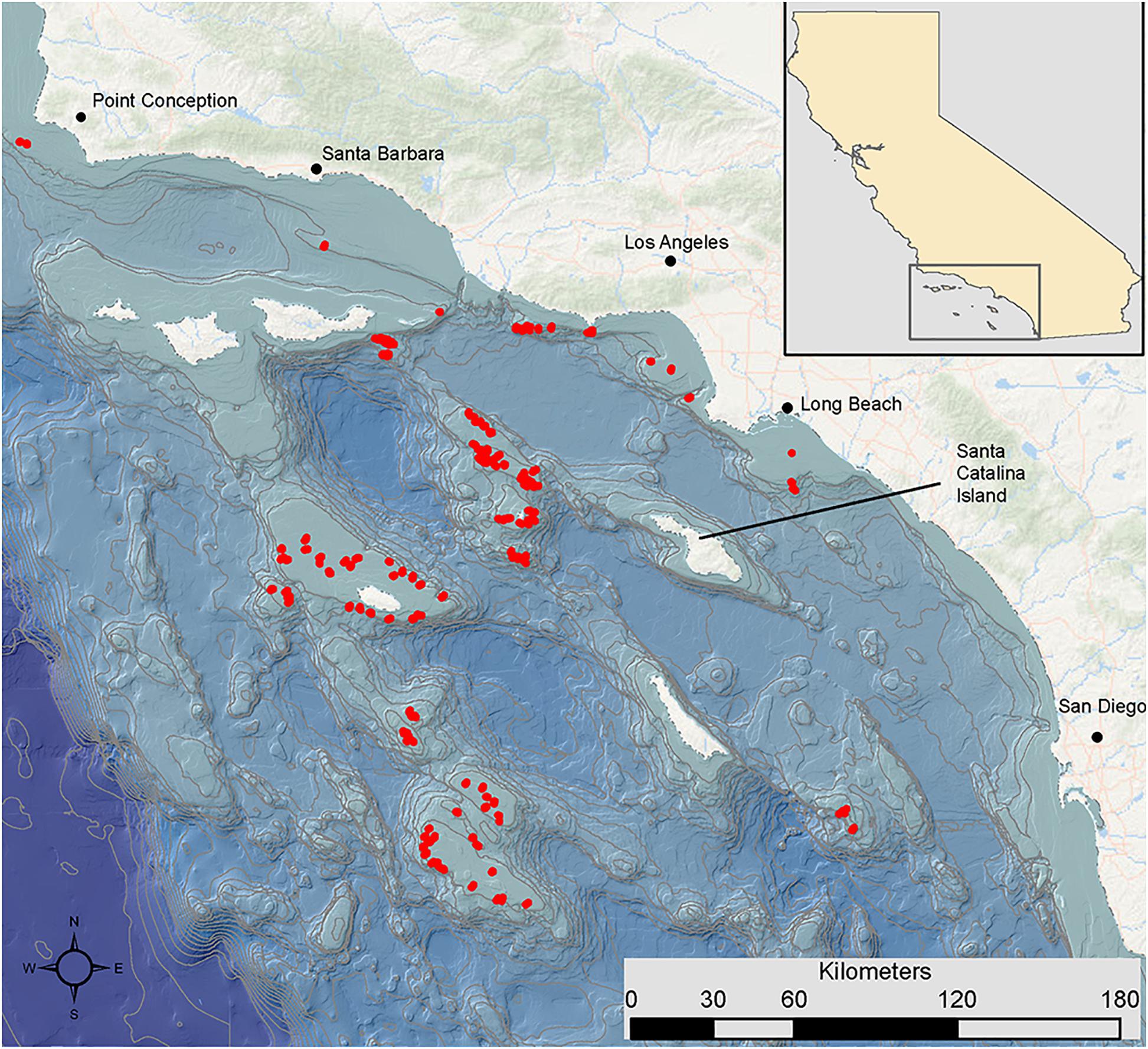
Figure 1. Map of the study area of the Southern California Bight off the coast of California (United States), with dive locations (red points) and 200 m depth contours (gray lines).

Seafloor habitat was characterized during the subsequent video analysis as the extent of substratum types and depth along each transect. Substratum types, comprised of pinnacle rock, boulder, rugose rock, cobble, gravel, pebble, flat rock, sand, and mud, were characterized along each transect by recording primary (>50% of the area) and secondary (>20% of the area) percent cover of each type based on review of the seafloor habitat visible in the video footage. We refer to each unique combination of primary and secondary substratum types along each transect as a patch. For the analyses, we also quantified the substratum types into a relative measure of “relief” based on the rough approximations used to classify each habitat. To do this, we extracted the minimum relief for each substratum type based on Greene et al. (1999; Supplementary Table 2) and summed the values of the primary and secondary habitat relief weighted by their percent cover (i.e., 0.5 for primary and 0.2 for secondary). Thus, we converted the categorical habitat classifications into a relative continuous substratum relief measurement.

Analysis Overview

To characterize associations between DSCS assemblages and demersal fishes, we conducted a series of multivariate analyses followed by fitting logistic regressions and gradient forest models to examine ecological correlates of fish presence. All analyses were conducted using the R programming language (R Core Team, 2019). We first used a cluster analysis to group habitats based on their DSCS assemblages. We then used both an indicator species analysis developed by Dufrene and Legendre (1997) and the “NbClust” package (Charrad et al., 2014) in R to determine the appropriate number of clusters necessary to describe the DSCS and fish assemblages. We then used a combination of random forest and logistic regression models to identify which physical and biological factors had the most influence on rockfishes (Sebastes spp.) density, distribution, and presence as well as to determine if any DSCS and fish taxa were statistically associated with each other while accounting for other physical (e.g., depth and substratum type) covariates. Finally, we used a gradient forest analysis to identify which of the ecological correlates used in the logistic regression analysis had the largest influence on fish biodiversity.

Cluster Analysis

To describe the DSCS assemblages, and improve the interpretability of the cluster analysis, we combined DSCS abundances for all patches of the same substratum type within 50 m depth bins. This unique combination of primary substratum (>50%), secondary substratum (>20%), and depth (hereafter referred to as a habitat unit) was the cluster analysis sample unit. For example, all patches that had boulder as a primary substratum type, rock as a secondary type, and were located at a depth between 100 and 150 m comprised the BR100 habitat unit. These habitat units were not spatially or temporally explicit (i.e., they were comprised of patches dispersed throughout the sample area and sampled anytime between 2002 and 2011), therefore we did not account for spatial or temporal autocorrelation at this stage in our analysis.

We then conducted a hierarchical cluster analysis on the Hellinger-transformed DSCS density data (Legendre and Gallagher, 2001). We calculated the density of DSCS by dividing the number of observed DSCS by patch area. Patch area was estimated as the length of each patch multiplied by transect width. Prior to conducting this cluster analysis, we removed four DSCS taxa that were not identified to a sufficient taxonomic level to contain any useful information (Supplementary Table 3). We used the Hellinger transformation for the cluster analysis because it had the best properties compared with other common multivariate transformations such as Wisconsin, frequency, range, and ubiquity (McCune et al., 2002). This conclusion was based on the “rankindex” function in the R package “vegan” using the Morista-Horn distance metric (Oksanen et al., 2017). Legendre and Gallagher (2001) showed that the Hellinger transformation had good statistical properties when compared to other common transformations used in multivariate transformation. The Morista-Horn distance metric is the recommended distance measure for ecological data due to its relative independence from sample size (Wolda, 1981). We conducted the cluster analysis using the “gaverage” agglomerative clustering algorithm in the R package “cluster” (Belbin et al., 1992; Maechler et al., 2017). The “gaverage” algorithm was referred to by Belbin et al. (1992) as the “flexible beta” and uses the Lance-Williams formula to specify how dissimilarities are computed. We used the default beta value of −0.1 as recommended by Belbin et al. (1992) for a general agglomerative hierarchical clustering strategy.

We next employed both the indicator species method and the “NbClust” package (Charrad et al., 2014) to determine how many clusters most appropriately described our observed data. We used the indicator species method of Dufrene and Legendre (1997) to determine which species were more often associated with a given cluster of habitat units then would be expected by chance. From the indicator species method, we were able to identify species found primarily in one cluster and present within the majority of habitat units of that cluster. Although taxa could be present in multiple clusters, they could only be an indicator species for a single cluster. This method can be used to select an appropriate number of clusters by sequentially increasing the number of clusters and quantifying the total number of indicator species that have a significant (p < 0.05, via Monte Carlo) association with any single cluster (McCune et al., 2002). Because our primary interest was identifying associations between fishes and DSCS assemblages, we quantified the number of fish taxa that were indicator species for a cluster of habitat units defined by the DSCS assemblages. As with the DSCS, prior to the analysis we removed fish taxa that were not demersal or were not identified to a sufficient taxonomic level to contain any useful information (n = 14, Supplementary Table 3). We then selected the number of habitat unit clusters that had the most significant indicator species (McCune et al., 2002). This analysis was conducted using the “multipatt” function in the R package “indicspecies” (De Caceres and Legendre, 2009).

We also used the “NbClust” function (Charrad et al., 2014) to explore the number of clusters recommended by other indices. The “NbClust” function uses 30 indices for determining the number of clusters by varying different combinations of clusters, distance measures, and clustering methods. We used the “kmeans” cluster method because (1) “gaverage” method was not available in “NbClust” and (2) it is an iterative approach to forming clusters and therefore less susceptible to chaining, or forming large clusters from poorly separated groups.

Logistic Regression

Our next objective was to identify which DSCS and rockfish taxa were associated with each other, and our first step was to use logistic regression models to estimate the probability of presence for individual fish taxa as a function of biotic and abiotic covariates in each habitat patch. In contrast to the cluster analysis, where our goal was to identify broad-scale assemblage associations, we used each individual patch as the sample unit for this analysis to ensure that any observed relationships were among fishes and DSCS in relatively close spatial proximity. When examining fish-habitat associations, both the spatial scale of the experimental unit and the choice of statistical model are important in determining the outcome (Sharma et al., 2012).

Because individual patches were our sample unit, we wanted to account for any potential spatial autocorrelation in fish distributions. Therefore, we fit our models using a hierarchical Bayesian framework that easily allowed us to add complexity and determine if the added complexity improved model fit. We fit our logistic regression models using the integrated nested Laplace approximation implemented with the R-INLA package (Lindgren and Rue, 2015). The R-INLA package uses the Matérn correlation function to estimate a spatial covariance matrix based on the distance between two sample locations and two estimated parameters (Zuur et al., 2017). The two estimated parameters are k, which is related to the range of spatial dependency, and s, which is a spatial variance parameter. To determine if spatial autocorrelation improved model fit, we compared the global model (the full model with all potential ecological covariates) with and without spatial autocorrelation using Watanabe’s information criterion (WAIC; Watanabe, 2013). The WAIC value of the model that included spatial autocorrelation had to be more than 4 units lower than the non-spatial model for the spatial model to be selected as the most parsimonious.

Potential ecological covariates included in the model were specific to each patch and included depth, temperature, salinity, substratum, percent DSCS cover, DSCS density, mean DSCS height, and the density of each DSCS taxon. Each of these covariates was selected a priori based on their hypothesized influence on fish presence. Percent DSCS cover was calculated as the total width of all DSCS species observed within a patch divided by the patch area. Although it is common to include measures of bathymetry to derive seafloor characteristics, such as the bathymetric position index (BPI), we chose to only use observations collected in situ and, thus, used our estimate of “relief” from the primary and secondary substratum type. Prior to fitting models, we examined the densities of all DSCS within the patches to determine if there was a minimum habitat patch size where DSCS densities might be biased. Based on this analysis, we removed all patches smaller than 3 m² (Supplementary Figure 1). Also prior to fitting models, we used pairwise Pearson correlations to quantify collinearity among variables and selected a single variable from any pair with a correlation over 0.7. Based on this analysis, we excluded temperature and salinity as covariates because they were collinear with depth. We also excluded any DSCS taxa that were observed in less than 1% of patches to avoid potential analysis issues that could be caused by small sample sizes.

Due to the large number of potential DSCS taxa that were candidates, we decided to use a random forest analysis as an initial screening method to eliminate ecological covariates that had a low likelihood of association with fish presence. To quote from Ellis et al. (2012), “a random forest (Breiman, 2001) is an ensemble of a large number of regression (or classification) trees, in which each tree is fit to a bootstrap sample (i.e., with replacement) of the observations, and each partition within a tree is split on the best of a random subsample of the predictor variables.” Random forests have generally performed better than other approaches to examine species distributions (Prasad et al., 2006) as well as fish-habitat relationships (Knudby et al., 2010). To account for the spatial nature of our analysis, we used a recently developed spatial extension of the random forest that accounts for the spatial dependency and heterogeneity in the data (Georganos et al., 2019). Although random forest is a valuable method for ranking relative variable importance, it is difficult to identify individual relationships between taxa. Because our ultimate goal was to provide managers with a prioritized list of DSCS taxa that were associated with fish taxa, we decided to use the random forest as an initial screening and use the logistic regression to identify the specific taxa that were most associated with the presence of individual fish taxa. After some preliminary examination of the data, we arbitrarily used two criteria to screen variables based on the spatial random forest results: (1) the maximum increase in mean squared error (MSE) was greater than 20 and (2) the percent increase in MSE (calculated as the increase in MSE multiplied by 100 divided by the MSE standard deviation) was greater than 15%.

The response of the logistic regression model was whether or not an individual fish taxon was present or absent within that patch. Thus, for each taxon (i) in each patch (j) our global model without spatial autocorrelation was:

$$\text{Logit}{(\mathrm{fish}\mathrm{pres})}_{\text{ij}}={\text{Depth}}_{\text{ij}}+{\text{Substratum}}_{\text{ij}}+{\text{Cover}}_{\text{ij}}$$

$$+{\text{Height}}_{\text{ij}}+{\text{Density}}_{\text{ij}}+{\mathrm{\epsilon }}_{ij}$$

Where the response was the logit transformed binomial of whether or not a fish was observed within a patch, depth was the mean depth of that patch measured along the transect, substratum was the continuous relative relief as calculated from the primary and secondary substratum types, Cover was the percent DSCS cover, Height was the mean height of all DSCS in each patch, Density was the densities of the DSCS taxa that could be associated with that fish taxa after the random forest screening, and e was the residual error. All fixed covariates were scaled (i.e., z-transformed) so that the model coefficient estimates were on a similar scale.

Our global model with spatial autocorrelation was nearly identical, but included an additional random effect (u) to account for spatial autocorrelation:

$$\text{Logit}{\left(\mathrm{fish}\mathrm{pres}\right)}_{\text{ij}}={\text{Depth}}_{\text{ij}}+{\text{Substratum}}_{\text{ij}}+{\text{Cover}}_{\text{ij}}$$

$$+{\text{Height}}_{\text{ij}}+{\text{Density}}_{\text{ij}}+u_{ij}+{\mathrm{\epsilon }}_{ij}$$

$$u_{ij}\sim GMRF(0,\text{Σ})$$

The spatial autocorrelation term (u) is assumed to have a random intercept and come from a Gaussian Markov random field (GMRF) with mean 0 and covariance matrix S. The covariance matrix (σ) is calculated using the two parameters (κ and σ) estimated by the Matérn correlation function.

We used WAIC to conduct model selection and used area under the curve to assess model performance. We conducted our model selection in two stages to ensure that we accounted for depth- and substratum-related covariates. Our first model selection stage included only depth, substratum, DSCS height, and DSCS cover (i.e., we excluded DSCS densities) and, thus, compared a maximum of 16 models. The purpose of this stage was to identify the physical and biological covariates that accounted for as much variation in fish presence as possible prior to including individual DSCS taxa. We selected the model with the fewest covariates and a delta WAIC values less than 4. We used Bayesian model averaging (Hoeting et al., 1999) if more than one model was selected based on those criteria. In the second model selection stage, we included all potential DSCS taxa in addition to the physical and biological covariates selected in the first stage. Covariate were considered important in estimating whether or not a fish was present within a habitat patch based on whether the 90% credible interval (90% CrI) of that covariate included zero, indicating there was no effect of that covariate on the response. The 90% CrI is the interval in which there is a 90% probability that the true (unknown) parameter estimate exists, given the observed data. During the second model selection stage, we removed any covariates that had 90% CrI that overlapped with zero. We refit the model after removing covariates with 90% CrIs that included zero, and repeated this process until all covariates had 90% CrIs that did not include zero or until there were no significant covariates remaining. We used the area under the receiver operating characteristic curve (AUC) method to gauge the adequacy of the model relative to the observed data (Hosmer et al., 2013).

We chose a subset of nine rockfish taxa that were either of high commercial value or conservation concern to present our logistic regression results. We downloaded commercial landing data for 2000–2017 from the National Oceanic and Atmospheric Administration website: https://foss.nmfs.noaa.gov/apexfoss/. We calculated the average landings in California for each species over that time period and merged those data with our dataset. We then selected the top five most landed rockfish species by pounds. In addition to those species, we included bocaccio (S. paucispinis), canary rockfish (S. pinniger), cowcod (S. levis), and young-of-year rockfish, as these taxa were of conservation interest due to current (or recent) protection status and the importance of young-of-year growth to maturity in the definition of essential fish habitat. To visualize the effect of each covariate, we calculated the probability of fish presence over the observed range (1–99% quantiles) of an individual covariate based on the logistic regression coefficient estimates and plotted these values against the individual covariate. To isolate the effect of that covariate on individual taxa, we constrained the other covariates to median values. We refer to these figures as “response plots.”

Gradient Forest Analysis

In addition to identifying the ecological covariates that are associated with an increased probability of fish presence, we also were interested in determining the covariates that increased fish biodiversity. We used gradient forest analysis (Ellis et al., 2012), which is a multivariate extension of the random forest method, to quantify multispecies responses to environmental gradients and to understand the drivers of differences in biodiversity (Pitcher et al., 2012). This method first uses a random forest to determine which covariates improve fit of the observations, and then uses a novel algorithm to determine the importance of each predicator for all species within a data set (Ellis et al., 2012; Pitcher et al., 2012). The gradient forest component collates the splits from each random forest along the gradient of each predictor (Ellis et al., 2012; Pitcher et al., 2012). See Ellis et al. (2012) for further statistical details regarding this approach. We ran the gradient forest for all observed fish taxa in the same patches as the logistic regression to determine which physical and biological variables had the largest influence fish biodiversity.

Results

Data Summary

There were general trends of primary substratum type and biological community with depth. After removing 51 small patches (<3 m²) from the dataset, and 29 habitat patches that were repeated in multiple surveys, we were left with 5144 habitat patches. We observed a mean of 10.53 ± 0.77 habitat patches on each transect and the mean size of each patch was 72.00 ± 3.42 m². The ratio of hard to soft primary substratum types declined from 57% at 50 m to 33% at 200 m (Figure 2). Between 200 and 350 m, the ratio of hard to soft substrata was approximately 50%.

FIGURE 2

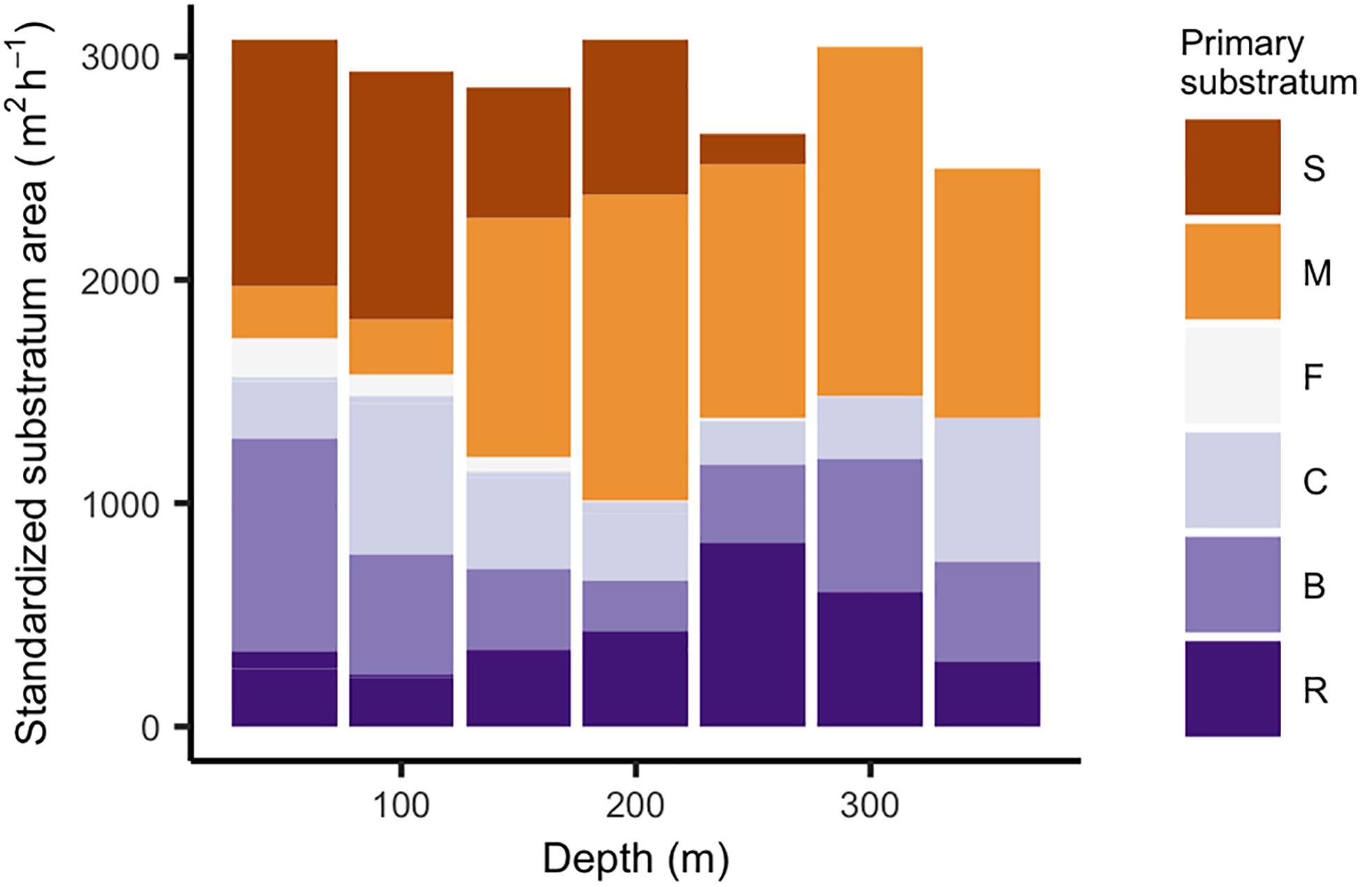
Figure 2. Area of soft (orange hues) and hard (purple hues) primary substratum types within 50-m depth bins. We standardized substratum areas (m²) by the number of survey hours (h) within each depth bin. Standardization was used because time at depth was variable. Substrata include sand (S), mud (M), cobble (C), boulder (B), rock (R). Three rarely observed substratum types were grouped with their closest substratum category based on relief. We categorized pinnacles with rock, and both pebbles and gravel with cobble.

The number of observed DSCS taxa was dependent on both substratum type and depth (Figure 3A). The highest number of DSCS taxa occurred when both primary and secondary substrata were hard. In these patches, the number of DSCS taxa peaked between 250 and 300 m. Soft habitat patches had lower numbers of DSCS taxa and did not co-vary with depth. There was a similar relationship between percent DSCS cover and substratum type and depth, although percent cover declined at deeper depths, whereas the number of species stayed relatively constant (Figure 3B). Patches dominated by hard substrata had the lowest DSCS cover at shallow and deep depths, with the peak DSCS cover between 200 and 250 m (Figure 3B). In contrast, DSCS height was greatest in soft substratum patches and declined with depth in all substratum types (Figure 3C). This was primarily the result of sea pens (Pennatulacea), which were among the tallest DSCS taxa observed (Table 1) and were abundant in the soft substratum patches. The density of fishes was greatest at shallow depths in hard substrata. As with DSCS height, fish density declined with depth (Figure 3D).

FIGURE 3

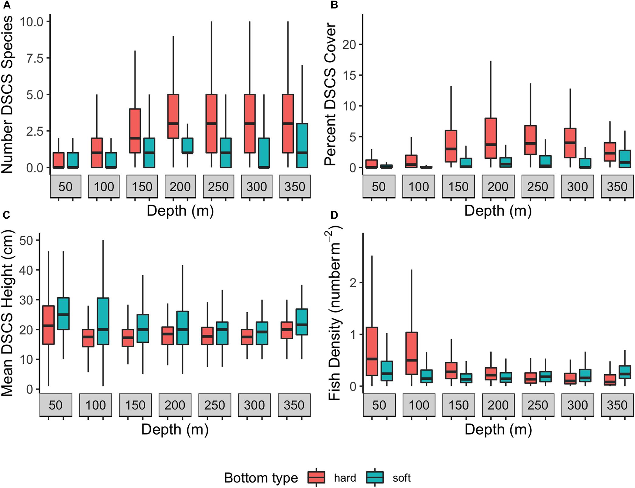
Figure 3. The (A) number of Deep-sea coral and sponge (DSCS) species, (B) percent DSCS cover, (C) mean DSCS height, and (D) fish density by depth in habitats with hard (pinnacle rock, boulder, rugose rock, cobble, gravel, pebble, flat rock) and soft (mud and sand) primary substratum types.

TABLE 1

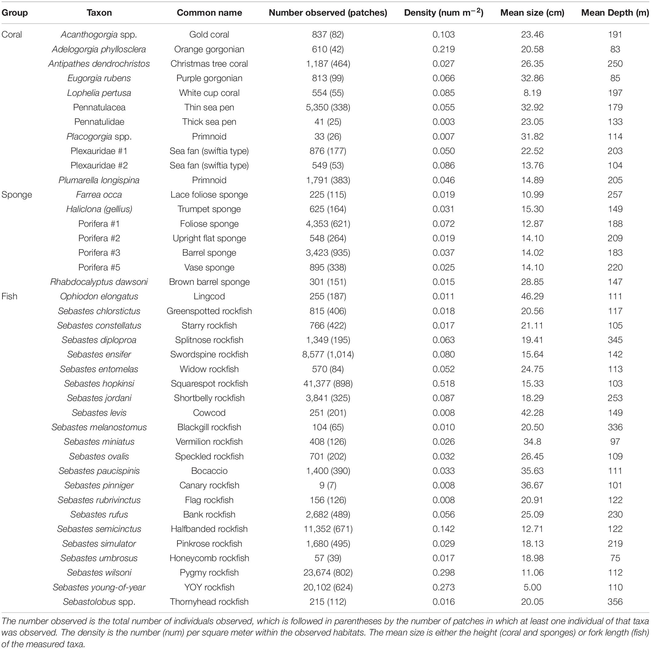
Table 1. Summary of observations of DSCS and fish taxa mentioned throughout text.

Cluster Analysis

The indicator species and “NbClust” methods suggested that our data was best described by four to six clusters (Figure 4). Clusters were defined by the density of DSCS taxa (matrix columns, n = 32) within each habitat unit (matrix rows, n = 213). Using the indicator species method, the maximum number of species was observed with either four or five clusters (Figure 4A). Eight of the indices from “NbClust” indicated that two clusters best describe our data, which we suspect was driven by difference between shallow and deep DSCS communities (Figure 4B). However, based on our ecological knowledge, we believe there are more differences in DSCS communities than those based simply on depth. The second mode from “NbClust” was at six clusters (Figure 4B), which was similar to that from the indicator species approach. Upon further examination, there was no ecological difference between the clusters formed when there was either four, five, or six clusters. The difference between four and five clusters was that some of the habitat units were removed from Cluster 1 and put into a separate cluster. However, this new cluster had no associated indicator species for fishes or DSCS, and therefore does not change our interpretation ecologically. The addition of a sixth cluster split the soft bottom habitat units into two separate clusters: one with thinner sea pens (Pennatulacea) as the indicator species and the other with thicker sea pens (Pennatulidae) as the indicator species. We think these two types of habitats were ecologically similar and should be in the same cluster. Therefore, we selected four clusters as most representative of the SCB.

FIGURE 4

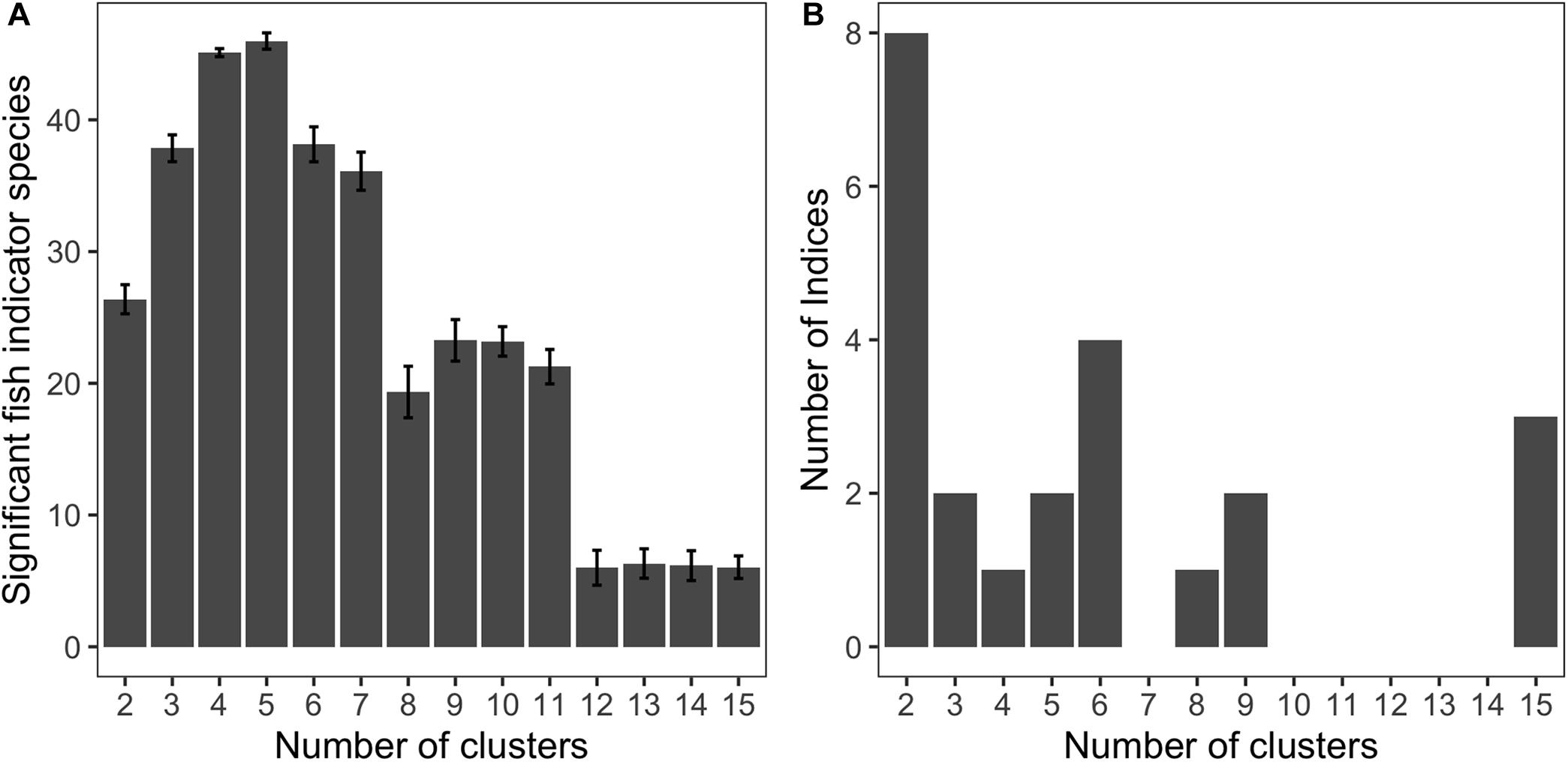
Figure 4. (A) The number of significant indicator fish species as a function of the number of clusters. The error bars were calculated by a Monte Carlo resampling approach to determine which taxa are indicator species for each cluster. (B) A histogram of the number of indices from the NbClust library that selected various number of clusters as the most appropriate based on the habitat unit data.

Habitat clusters were primarily differentiated by their depth and substratum, and they contained a wide range of indicator species in different taxa (Table 2). Clusters 1 and 2 primarily consisted of hard or mixed substratum types found within the 100–300 m depth range (Table 2). Cluster 3 comprised hard and mixed substratum types in the shallowest depths (50 m). Fishes in the Sebastes genus dominated the significant indicator fish species in the first three clusters. The DSCS taxa in the first three clusters primarily were gorgonians from the order Alcyonacea. Notably, Cluster 2 also contained a single species of black coral and a single species of Scleractinian coral, Antipathes dendrochristos (Christmas tree coral) and Lophelia pertusa (white cup coral), respectively. Cluster 4 primarily comprised soft substrata at depths from 100 to 300 m. The fish indicator species in Cluster 4 were primarily flatfish, sculpins, combfish, eelpout, poachers, and pricklebacks. The two indicator DSCS species for this cluster were both corals commonly known as sea pens (order Pennatulacea).

TABLE 2

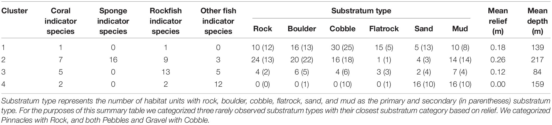
Table 2. Description of the fish and substratum types found within each of four DSCS clusters.

The four clusters were defined both by the density of DSCS within the habitat units and the density of DSCS taxa within the cluster (Figure 5). Clusters 3 and 4 were clearly defined by their indicator DSCS taxa, whereas the indicator species in Clusters 1 and 2 were less dominant throughout the habitat units in those clusters. However, Cluster 2 had the most DSCS indicator species of any cluster. Cluster 3 included the shallowest habitat units and was well defined by five indicator DSCS taxa that were found in much higher abundance in the habitat units within this cluster than in any other habitat units: Plexauridae #2 (sea fan), Placogorgia sp. (primnoid), Adelogorgia phyllosclera (Orange gorgonian), Eugorgia rubens (Purple gorgonian), and Leptogorgia chilensis (Red gorgonian). Likewise, the soft bottom Cluster 4 was well defined by Pennatulidae and Pennatulacea, which are both sea pen taxa. In contrast, there were some sponges (Porifera #2, #3, and #5) that were found in both Clusters 1 and 2 (the deeper clusters with high substratum relief) in nearly equal abundances. Table 1 provides descriptions of the observed size, depth, and abundances of these DSCS taxa.

FIGURE 5

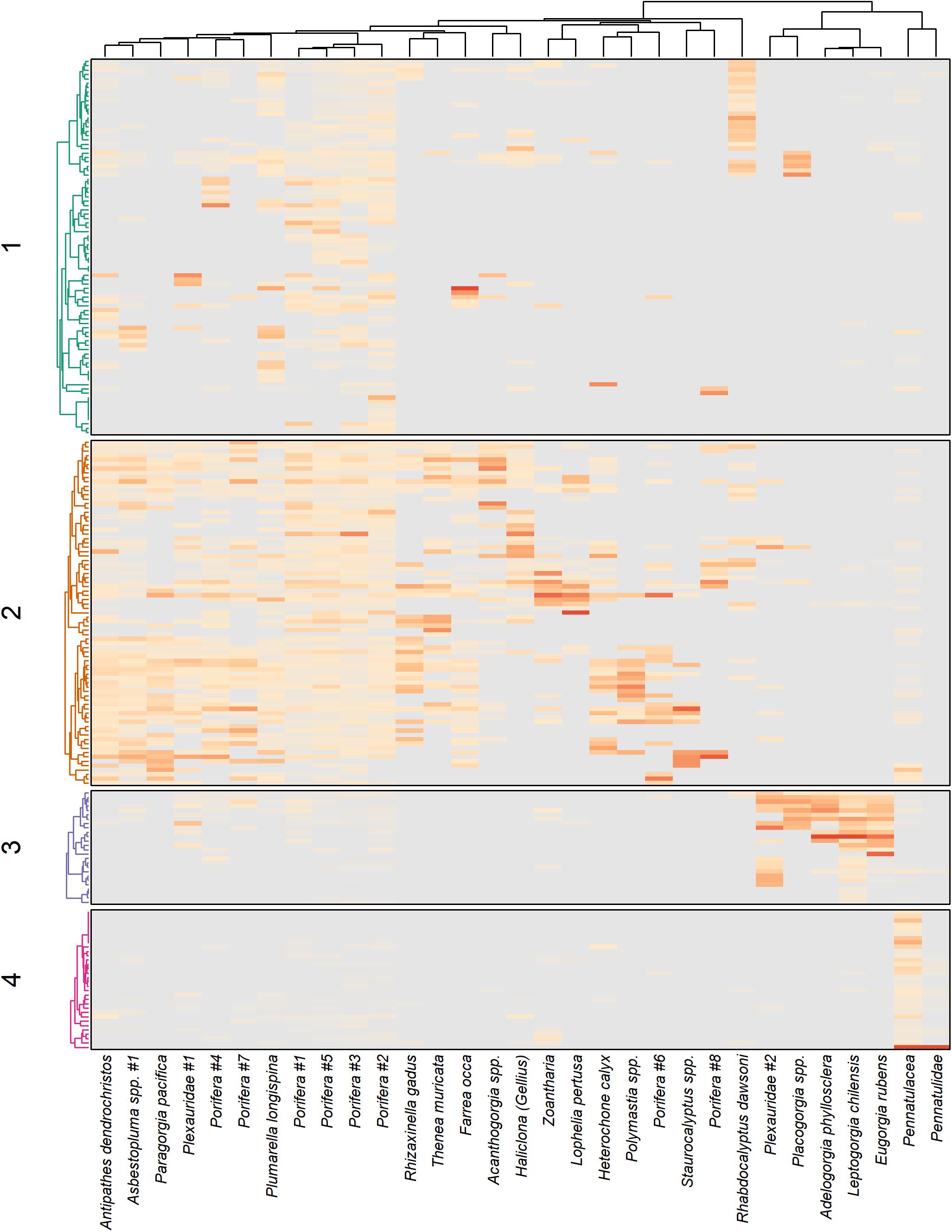
Figure 5. Density (darker colors represent higher densities) of DSCS taxa within each of four clusters. Dendrograms on the left-hand side represent the classification of the habitat units (defined as the combination of primary and secondary substratum type together with 50 m depth bin). The large number of habitat units cannot be individually labeled, but the general classifications for each cluster are described in the text.

Logistic Regression

From the logistic regression analysis, depth and coral height were the primary ecological covariates correlated with the increased probability of fish presence within habitat patches. The vast majority (43 of 45; 96%) of the fish taxa were better represented by models that included a spatial correlation term. Thus, fishes within these taxa were more likely to be present in patches closer to one another. Water depth was included as an important covariate in 76% (34 of 45) of the models (Supplementary Table 4). As expected, the fish taxa could be categorized into fishes found in deeper water (positive depth odds ratio) or fishes in shallower water (negative depth odds ratio). DSCS height also was included in a large percentage (30 of 45; 67%) of fish taxa models. In contrast to water depth, all of the fishes had positive DSCS height odds ratios, indicating that fishes were more likely to be present in patches with taller-than-average DSCS. Interestingly, this correlation only became clear after we included the spatial correlation term in the models. The correlation between DSCS height and fish presence depended on which cluster the fishes were associated with. The vast majority of models (86%) for fishes in Cluster 4 included the DSCS height term, whereas only 36% of models for fishes in Cluster 2 included this term. Because Cluster 4 represents habitats with softer sediments without much relief except the exceptionally tall sea pens, it is intuitive that fishes in these habitats would more likely associate with taller corals. Although substratum was included in 58% of the logistic regression models, there was not an obvious pattern of how substratum was related to fish presence. Only 10 of the 45 fishes (22%) had models with a positive odds ratio for substratum, implying that our measure of substratum relief was not a major driving factor in predicting fish presence for most taxa. There also were 16 taxa that had a negative substratum odds ratio, and 11 of those fishes (69%) were in Cluster 4. DSCS cover was only included in 22% of logistic regression models and had a negative odds ratio in all the models it was found in except one (Supplementary Table 4). As with substratum, the majority (67%) of fishes with logistic regression models that included DSCS cover were in Cluster 4.

A few key DSCS taxa were associated with fish presence, after accounting for depth, DSCS height, DSCS cover, and substratum (Table 3). The DSCS taxa that recurred in the most logistic regression models were sponges in the phylum Porifera. These sponges were important for multiple rockfish species (Table 2) as well as lingcod (Ophiodon elongatus) (Supplementary Table 4). Multiple coral taxa were positively associated with the increased probability of fish presence. In contrast to the sponge taxa, the coral taxa tended to be associated with only one or two fish taxa (Table 2). The results from the logistic regression models also suggest that the densities of DSCS taxa were less likely to affect the presence of rockfish taxa in deeper habitats. Most (11 of 14, 79%) of the rockfish taxa that had a negative depth odds ratio in their logistic regression models (i.e., they were more likely to be found in shallower depths) also had a positive association with the densities of at least one DSCS taxa. In contrast, none of the seven rockfish taxa that had positive depth odds ratios had a positive association with any DSCS taxa.

TABLE 3

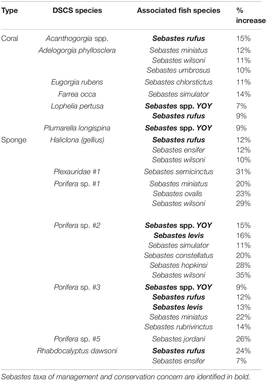
Table 3. Associated DSCS and Sebastes taxa and the percent increase in the probability of fish presence with a standard deviation increase in DSCS abundance based on the logistic regression models.

The top five rockfish taxa landed by pounds in commercial fisheries, and observed within at least 1% of patches in our dataset, were thornyhead (Sebastolobus spp.) (846,152 lbs), blackgill rockfish (S. melanostomus) (214,554 lbs), widow rockfish (S. entomelas) (152,604 lbs), bank rockfish (S. rufus) (137,770 lbs), and splitnose rockfish (S. diploproa) (98,722 lbs). Bank rockfish was the only one of these top commercially landed taxa that was positively associated with any DSCS taxa (Table 3). Both bank rockfish and widow rockfish were the only two of these five taxa found in shallower depths (i.e., negative depth odds ratios). As previously mentioned, the deeper rockfish taxa generally were not positively associated with DSCS taxa. The taxa of conservation interest we selected were young-of-year rockfish, cowcod, bocaccio, and canary rockfish. We were unable to fit a reasonable model for canary rockfish using these ecological covariates. For the other three conservation taxa, DSCS height was positively correlated with the probability of fish presence, where substratum was only correlated with bocaccio (Figure 6 and Table 4). Both young-of-year rockfish and cowcod were positively associated with multiple DSCS taxa (Figure 6 and Table 4).

FIGURE 6

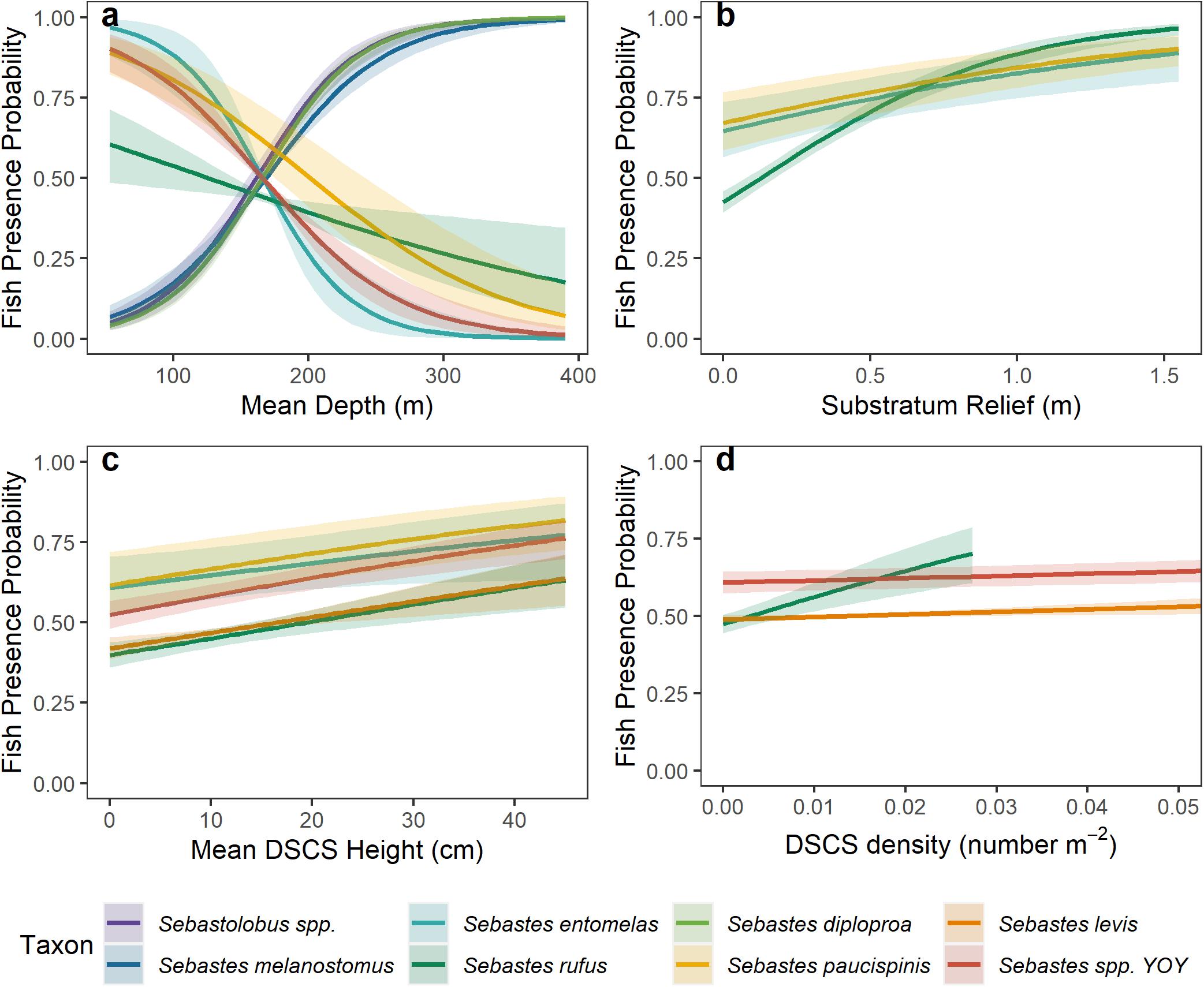
Figure 6. Response plots of the probability of fish presence relative to (A) Mean Depth, (B) Substratum Relief, (C) Mean DSCS Height, and (D) DSCS density based on results from the covariates included in the logistic regression. No line is shown if a covariate was not included in the best model for that fish taxon. In (D) we only plot the relationship for DSCS taxa with the largest response greater than zero, because we were interested only in taxa that increased the probability of taxon presence.

TABLE 4

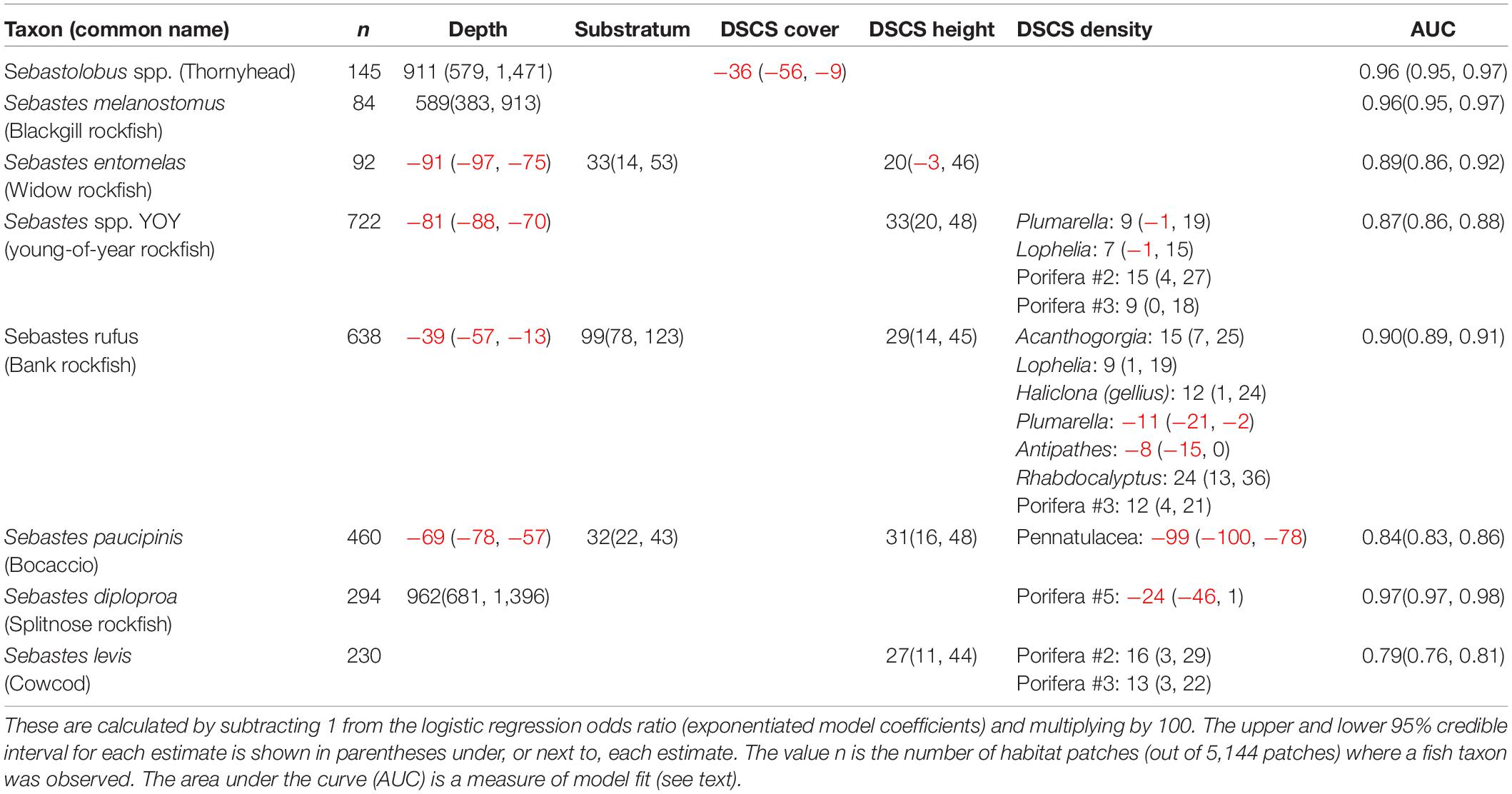
Table 4. Results of logistic regression showing the percent increase (black), or decrease (red), in the probability of fish presence with a standard deviation increase in each covariate.

Gradient Forest

The gradient forest analysis generally supported the results from the logistic regression and indicated that depth and ecological covariates related to DSCS were the primary factors that influenced the biodiversity of demersal taxa throughout the SCB. Using the gradient forest method, the importance of each predictor can be evaluated based on their contributions to the accuracy importance (R²) for each random forest and averaged across all species to provide an overall importance (see Ellis et al., 2012 for statistical details). Although we originally hypothesized that depth and substratum would be the strongest predictors of biodiversity, it was actually depth and percent DSCS cover that were the strongest predictors (Figure 7). Many of the same DSCS taxa that were associated with increased presence of fish taxa based on the logistic regression models also were associated with increased fish biodiversity based on the gradient forest. In fact, 6 of the top 10 DSCS taxa from the gradient forest (selected out of 39 potential DSCS taxa) were those also associated with increased probability of fish presence based on the logistic regression (Table 3 and Figure 7).

FIGURE 7

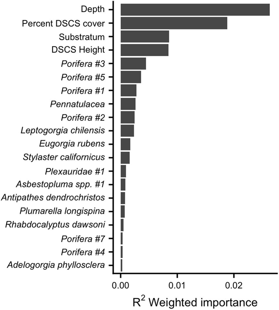
Figure 7. Gradient forest estimated relative importance of physical and biological covariates for predicting biodiversity of fish taxa in the SCB. Note that for clarity we have displayed only the top 20 covariates out of a total of 43.

Interesting patterns relative to depth and coral height were evident from a plot of the ratio of forest splits to observed data along the gradient of these variables (Figure 8). Locations on the gradient where splits density was greater than data density (Figure 8: blue line ratio > 1) indicate higher relative importance for species composition change (Pitcher et al., 2012). Note that because these values are standardized by the observed data, they represent the density of the random forest splits corrected for sampling bias. The depth results indicate that shallow depths (<100 m) and deeper depths (>250 m) have the greatest relative importance for species compositional change (Figure 8A). Likewise, DSCS taxa between 5 and 60 cm have the greatest relative importance for compositional change (Figure 8C). No clear patterns were apparent for percent DSCS cover or substratum.

FIGURE 8

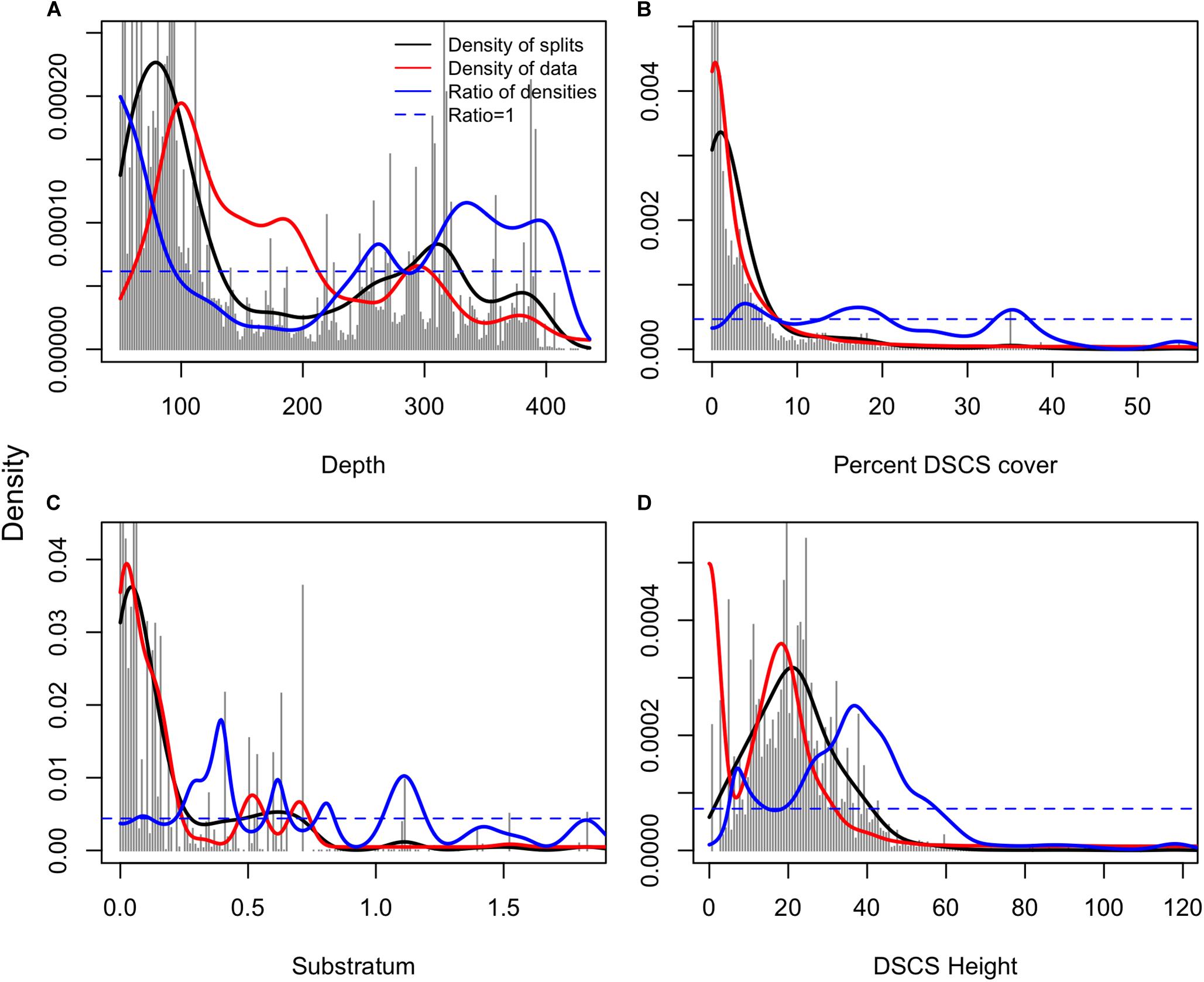
Figure 8. Gradient forest output showing the locations of the random forest splits (gray bars), densities of splits (black line), densities of observations (red line), and the ratio of splits standardized by observation density (blue line). Ratio > 1 indicate locations of relative greater change in composition. Note that the panels are on different scales based on the number of bins the data is split between for each variable.

The cumulative importance plots revealed varying levels of association between various rockfish taxa and each of the DSCS taxa (Figure 9). Some rockfish taxa were strongly associated with one DSCS taxon well beyond any of the other rockfish taxa. For example, bank rockfish and swordspine rockfish (S. ensifer) exhibited a strong association with Acanthogorgia spp. (gold coral). Although both fish taxa responded strongly to Acanthogorgia spp., it took larger densities of this DSCS taxa before the probability of bank rockfish presence increased compared with swordspine rockfish. This was indicated by a steep cumulative importance curve as the density of Acanthogorgia spp. increased, while most other fish taxa cumulative importance curves remained close to zero and relatively constant (Figure 9A). In contrast, the probability of fish presence increased for most fish taxa with increasing densities of Porifera #2 (Figure 9B). For most taxa, this increase occurred as Porifera #2 densities reached 0.05–0.15 individuals per m². Note there is an order of magnitude difference in the y-axis scale for the plots of these two DSCS taxa. This illustrates why Porifera #2 was ranked as the 4th most important DSCS taxa while Acanthogorgia spp. was the 19th most important DSCS taxa and does not even appear in Figure 7.

FIGURE 9

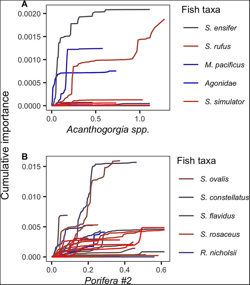
Figure 9. Cumulative importance distributions of standardized random forest splits for each fish taxa (individual lines) along the observed density gradient for (A) Acanthogorgia spp. and (B) Porifera #2.

Discussion

We described four communities of deep-sea coral, sponge, and fish assemblages in the SCB, and demonstrated that the density of DSCS taxa increased the probability of presence for multiple fish taxa and increased fish biodiversity. The results from two different analytical approaches indicated the same DSCS taxa were correlated with fish taxa in the SCB, which strongly suggests that these DSCS taxa play an important role in the ecosystem. From the logistic regression analysis, it was evident that increased densities of DSCS taxa increased the probability of at least three rockfish taxa of management and conservation interest, including young-of-year rockfish. These fish taxa occupy DSCS habitat potentially because DSCS provide benefits such as increased prey density (Quattrini et al., 2012), predation refuge (Krieger and Wing, 2002; Costello et al., 2005), and nursery habitat (Stone, 2006, 2014; Baillon et al., 2012).

Our finding that young-of-the-year rockfish are more likely to occur in habitat patches with taller DSCS supports the suggestion that DSCS can provide important nursery habitats for these taxa (Edinger et al., 2007; Harter et al., 2009; Baillon et al., 2012). Specifically, our results suggest that young-of-the-year rockfish were more likely to be present in habitat patches with increased densities of Lophelia pertusa (7%), Plumarella longispina (9%), Porifera #2 (15%), and Porifera #3 (9%). In addition to the association with these specific taxa, the model also indicated that young-of-the-year rockfish were more likely to be present in patches with taller corals. Baillon et al. (2012) also observed Atlantic Sebastes larvae associated with deep-sea coral, implying that they use these habitats as nursery grounds. Multiple authors have noted the presence of gravid Sebastes near Lophelia reefs (Fosså et al., 2000 cited in Husebø et al., 2002; Costello et al., 2005), suggesting they may release their young near these reefs. However, we note that Lophelia has a much different reef-forming pattern in the Atlantic (where these previous studies were conducted) than in the Pacific so it is best not to assume that fishes are using these corals in the same way. The use of DSCS by gravid Sebastes may be due to the protection these corals provide from predators (Krieger and Wing, 2002; Costello et al., 2005) or the additional feeding opportunities, because researchers anecdotally have noted that zooplankton abundances are higher near DSCS (Costello et al., 2005). Although our study cannot establish why young-of-year rockfish are using these DSCS habitats, our results imply that DSCS are important to these fishes growth to maturity, which supports the classification of DSCS as essential fish habitat (Rosenberg et al., 2000). Similarly, a modeling study in the Northeast Atlantic (Foley et al., 2010) also concluded that Sebastes population dynamics were important to the intrinsic growth rate of the stock. Their results were consistent with corals serving as essential fish habitat and suggested that coral removal would result in the decline, and potential extirpation, of some Sebastes populations.

Our analytical approach also identified some specific DSCS taxa that were associated with demersal fishes, and we suggest species distribution maps should be developed for these taxa to ensure they are protected from future damaging human practices (e.g., benthic trawling). Deep-sea coral taxa are slow growing, so it can take a long time for them to recover once they have been damaged (Roberts et al., 2006; Althaus et al., 2009). Consequently, it is important to identify locations where these taxa may be found in the highest densities, validate their presence, and provide protection to these areas before any further damage is inflicted. Species distribution models are one method to identify the areas where taxa are expected to be found based on sample observations. Species distribution models have been developed for multiple DSCS taxa to examine the factors that influence habitat suitability at a variety of scales. Multiple authors have developed species distribution models to predict global habitat suitability for various DSCS taxa (Tittensor et al., 2009; Davies and Guinotte, 2011; Yesson et al., 2012). In general, these models have predicted that the majority of suitable coral habitat was on the continental shelves and slopes of the Atlantic, South Pacific, and Indian Oceans as well as seamounts along the northern Mid-Atlantic Ridge and in the South Pacific Ocean. Models developed at finer scales are perhaps more useful to identify areas that could be protected from anthropogenic practices that may potentially damage these fragile DSCS taxa (Rengstorf et al., 2013; Gullage et al., 2017; Sundahl et al., 2020). For example, Huff et al. (2013) found that the distribution of the Christmas tree coral in the SCB (Antipathes dendrochristos) was positively affected by a combination of persistently high surface productivity, water current velocity and direction near the seafloor, warmer temperature and shallow depth. Developing similar distribution maps for the other DSCS taxa associated with demersal fishes would be invaluable to fisheries managers seeking to protect these vulnerable fish habitats as they seek to rebuild overfished populations (Rosenberg et al., 2000).

The logistic regression analysis indicated that the probability of fishes being associated with DSCS was primarily related to depth, and we did not find that this association was as highly related to substratum relief as we anticipated. All the fish taxa that had positive relationships with DSCS taxa were found in depths shallower than 230 m, while all the fish taxa at mean depths greater than 300 m generally had no, or negative, relationships with DSCS taxa. One explanation for this is that at deeper depths DSCS cover decreases (Figure 3). Therefore, we are less likely to see fishes and DSCS on the same transect, or in the same patch, unless we have a sufficiently high sample size. Unfortunately, the fish taxa with deeper mean depths had smaller sample sizes, thus we cannot say if there was an ecological reason why fishes at deeper depths were not associated with DSCS taxa (e.g., reduced need for predation refuge at depth) or if this was an artifact due to reduced sampling effort at deeper depths. We suspect that the probability of fish presence was correlated with relief for only a few taxa was likely due to the way we calculated relief from visual estimates of the primary and secondary substratum. Future surveys should consider simultaneously collecting bathymetry data (e.g., side-scan or multibeam sonar) to better correlate relief to fishes and invertebrate habitat.

Results from the gradient forest analysis revealed both expected and surprising relationships between fish biodiversity and various physical and biological covariates. Depth and DSCS cover had the largest influence on rockfish biodiversity in habitat patches. It was not surprising that depth was important, as we know that various taxa have specific depth preferences. Based on the results of the logistic regression, it was surprising that DSCS cover was considerably more important than either DSCS height or substratum type. This may have been due to the taxa that were included in this analysis (all 111 fish taxa were included in the gradient forest biodiversity analysis while just the significant indicator species were included in the logistic regression analysis), the fact that the gradient forest did not explicitly account for spatial autocorrelation as was done in the logistic regression, or simply that the two analyses were measuring different responses (univariate vs. multivariate). In any case, it is intuitive that fish diversity would increase as coral cover increases, as fishes generally associate with habitats having increased cover. It also is noteworthy that six of the top ten DSCS taxa selected from the gradient forest analysis (out of 39 possible taxa) also increased the probability of rockfish presence based on the results from the logistic regressions (Table 3). This suggests that some of the other DSCS taxa that were near the top of the gradient forest analysis (e.g., Pennatulacea and Antipathes dendrochristos) also may have important habitat roles for other taxa that were not included in our logistic regression models. Habitats with persistent localized upwelling resulting from complex seafloor topography are areas where Antipathes dendrochristos are denser (Huff et al., 2013), and also may comprise the most important benthic habitats for other DSCS and fishes in the SCB.

As with any survey method, there are weaknesses of using submersible observations to record species data that can potentially bias results. Behavioral reactions of fishes to submersibles have been documented, including avoidance, attraction, and no reaction (Stoner et al., 2008; Laidig et al., 2012; Sward et al., 2019). As Sward et al. (2019) state in their review of ROV surveys for visually assessing fish assemblages: “the type and severity of the reaction to the ROV can be influenced by a variety of factors, including the species, trophic position, and the body size and position of the individual relative to the seafloor as well as to different aspects of the ROV system (i.e., artificial lighting, thruster noise, speed).” Laidig et al. (2012) found that a smaller percentage of fishes (11%) reacted to the larger, manned submersibles (as we used in this study) than to ROVs (57%). Those fishes that did react to the manned submersibles tended to be smaller fishes, suggesting that it is more difficult to accurately count these smaller fishes (Laidig et al., 2012). Likewise, it is likely that the observers overlooked cryptic species that were able to hide among rocks, DSCS, and sediment. We would expect this bias to increase relative to the complexity of the habitat, although we are unaware of any studies that have conducted experiments to quantify this potential bias. Stoner et al. (2008) qualitatively noted that the reaction of most rockfish species was relatively low and concluded that bias was probably minimal. Finally, although the distribution of many species is influenced by time of day (Hart et al., 2010), our study only examined movement during the day. In their review, Sward et al. (2019) found that very few submersible studies (∼2%) were conducted at night. Telemetry studies have indicated that home ranges and behavior of Pacific rockfishes change both diurnally and seasonally (Tolimieri et al., 2009; Zhang et al., 2015). A quantitative comparison of diel habitat use using submersible video surveys would be an excellent future study.

Another area of future research is understanding the trophic dynamics of these DSCS habitats. Our results indicate that DSCS provide important habitat for multiple rockfish taxa, but we cannot identify what functional benefit these structure-forming invertebrates provide to the associated fishes. These DSCS may be found in areas where the hydrodynamics enhance the density of zooplankton and other potential prey items, some of which may be reliant on the DSCS (Husebø et al., 2002; George et al., 2007; Lessard-Pilon et al., 2010; Huff et al., 2013). Based on simplified trophic ecosystem models for deep-sea coral reef ecosystems, George et al. (2007) concluded that the degradation of corals and sponges would negatively impact populations of commercially important fish species. Thus, to understand the functional benefit of DSCS to fish populations, it would be valuable to compare diets of fishes in areas of high DSCS density and nearby habitats that have lower DSCS densities, such as those that have been disturbed by trawl fisheries.

Furthermore, future research could improve upon our results by incorporating a temporal component to the associations between fishes and DSCS taxa and by incorporating a measure of fishing impact as an additional covariate. Although DSCS generally are long-lived, and thus large changes in their distribution would not be expected over a short time scale, regional climatic variations (e.g., El Nino and ocean warming) can affect fish recruitment and distribution. These changes in the distribution and abundance of fishes could influence the interpretation of the observed associations between fishes and DSCS. Additionally, acute and rapid change in DSCS distribution can be caused by the impacts of benthic trawling (Yoklavich et al., 2018). For example, Clark and Rowden (2009) found differences in macro-invertebrate assemblages between fished and unfished seamounts in New Zealand. Future development of habitat suitability models could include amount of benthic trawling as a measure of habitat alteration. Continuing to collect long-term datasets of these deep-sea habitats and associated assemblages will help to understand the ecological importance of DSCS.

This study has provided evidence of the importance of DSCS as habitat for multiple taxa of fishes, including some with commercial importance, and re-enforces the importance of conserving these important structure-forming invertebrates. Previous research on structure-forming deep-sea invertebrates primarily focused on larger species, and our results highlight the importance of sponges that are generally overlooked as habitat forming invertebrates. Sponges are often the largest structure-forming invertebrates in their associated habitats, and provide considerable biotic complexity, predator refuge, and enhanced food supply (Tissot et al., 2006; Buhl-Mortensen et al., 2010).

DSCS taxa throughout the world’s seas are threatened by multiple factors. The impacts of fishing gear, primarily benthic trawling, have been documented on deep-sea reefs along the West Ireland continental shelf break (Hall-Spencer et al., 2002), Norway (Fosså et al., 2002), Tasmania (Koslow et al., 2001), and Alaska (Krieger and Wing, 2002; Heifetz et al., 2009). DSCS also are threatened due to climate change. A recent study estimated there would be no suitable habitat for deep-sea coral by 2099 assuming an upper temperature tolerance of 7°C (Thresher et al., 2015). Likewise, ocean acidification due to an increasing production of anthropogenic CO₂ has resulted in declining aragonite and calcite saturation states, which may impair the ability of DSCS taxa to build sufficiently robust skeletons (Guinotte et al., 2006). In the face of these potential threats, further conservation efforts are essential to protect these ecologically important DSCS.

Data Availability Statement

The raw data supporting the conclusions of this article will be made available by the authors, without undue reservation, to any qualified researcher.

Ethics Statement

Ethical review and approval was not required for the animal study because it was an observation only study.

Author Contributions

MY contributed the data and essential background for the study. MH and DH conceived the analysis. MH conducted the statistical analysis and prepared result figures. All authors conceived the study, contributed to writing, editing, and approved the submitted manuscript.

Funding

The authors would like to acknowledge the NMFS Office of Habitat Conservation Deep Sea Coral Research and Technology Program for funding portions of this research.

Conflict of Interest

The authors declare that the research was conducted in the absence of any commercial or financial relationships that could be construed as a potential conflict of interest.

Acknowledgments

We thank Tom Laidig, Linda Snook, and Mary Nishimoto for analyzing the visual surveys, and Tom Laidig and Diana Watters for maintaining the databases used in this study. We also thank Tom Hourigan, Chris Rooper, and four reviewers for reviewing early drafts of the manuscript and providing comments that greatly improved the final product. We appreciate the assistance of many experts in the identification of deep-sea corals and sponges. Any use of trade, product, or firm names is for descriptive purposes only and does not imply endorsement by the U.S. Government.

Supplementary Material

The Supplementary Material for this article can be found online at: https://www.frontiersin.org/articles/10.3389/fmars.2020.593844/full#supplementary-material

References

Addamo, A. M., Vertino, A., Stolarski, J., García-Jiménez, R., Taviani, M., and Machordom, A. (2016). Merging scleractinian genera: the overwhelming genetic similarity between solitary Desmophyllum and colonial Lophelia. BMC Evol. Biol. 16:108. doi: 10.1186/s12862-016-0654-8

PubMed Abstract | CrossRef Full Text | Google Scholar

Althaus, F., William, A., Schlacher, T. A., Kloser, R. J., Green, M. A., Barker, B. A., et al. (2009). Impacts of bottom trawling on deep-coral ecosystems of seamounts are long-lasting. Mar. Ecol. Prog. Ser. 397, 279–294. doi: 10.3354/meps08248

CrossRef Full Text | Google Scholar

Auster, P. J. (2005). “Are deep-water corals important habitats for fishes?,” in Cold-water corals and ecosystems, eds A. Freiwald and J. M. Roberts (Berlin: Springer), 747–760. doi: 10.1007/3-540-27673-4_39

CrossRef Full Text | Google Scholar

Baillon, S., Hamel, J.-F., Wareham, V. E., and Mercier, A. (2012). Deep cold-water corals as nurseries for fish larvae. Front. Ecol. Environ. 10, 351–356. doi: 10.1890/120022

CrossRef Full Text | Google Scholar

Belbin, L., Faith, D. P., and Milligan, G. W. (1992). A comparison of two approaches to beta-flexible clustering. Multivar. Behav. Res. 27, 417–433. doi: 10.1207/s15327906mbr2703_6

PubMed Abstract | CrossRef Full Text | Google Scholar

Bowden, D. A., Rowden, A. A., Leduc, D., Beaumont, J., and Clark, M. R. (2016). Deep-sea seabed habitats: Do they support distinct mega-epifaunal communitites that have different vulnerabilities to anthropogenic disturbance? Deep Sea Res. I 107, 31–47. doi: 10.1016/j.dsr.2015.10.011

CrossRef Full Text | Google Scholar

Breiman, L. (2001). Random forests. Machine Learning 45, 5–32.

Google Scholar

Buhl-Mortensen, L., Vareusel, A., Gooday, A. J., Levin, L. A., Priede, I. G., Buhl-Mortensen, P., et al. (2010). Biological structures as a source of habitat heterogeneity and biodiversity on the deep ocean margins. Mar. Ecol. 31, 21–50. doi: 10.1111/j.1439-0485.2010.00359.x

CrossRef Full Text | Google Scholar

Charrad, M., Ghazzali, N., Bioteau, V., and Niknafs, A. (2014). NbClust: An R package for determining the relevant number of clusters in a data set. J. Statist. Soft. 61, 1–36.

Google Scholar

Clark, M. R., and Rowden, A. A. (2009). Effect of deepwater trawling on the macro-invertebrate assemblages of seamounts on the Chatham Rise. N Z. Deep Sea Res. I 56, 1540–1554. doi: 10.1016/j.dsr.2009.04.015

CrossRef Full Text | Google Scholar

Core Team. (2019). R: A language and environment for statistical computing. R Foundation for Statistical Computing. Vienna: R Core Team.

Google Scholar

Costello, M. J., McCrea, M., Freiwald, A., Lundalv, T., Jonsson, L., Brett, B. J., et al. (2005). “Role of cold-water Lophelia pertusa coral reefs as fish habitat in the NE Atlantic,” in Cold-water corals and ecosystems, eds A. Freiwald and J. M. Roberts (Berlin: Springer), 771–805. doi: 10.1007/3-540-27673-4_41

CrossRef Full Text | Google Scholar

D’Onghia, G., Maiorana, P., Sion, L., Giove, A., Capezzuto, F., Carlucci, R., et al. (2010). Effects of deep-water coral banks on the abundance and size structure of the megafauna in the Mediterranean Sea. Deep Sea Res. II 57, 397–411. doi: 10.1016/j.dsr2.2009.08.022

CrossRef Full Text | Google Scholar

D’Onghia, G., Maiorano, P., Carlucci, R., Capezzuto, F., Carluccio, A., Tursi, A., et al. (2012). Comparing deep-sea fish fauna between coral and non-coral ‘megahabitats’ in the Santa Maria di Leuca cold-water coral province (Mediterranean Sea). PLoS One 7:e44509. doi: 10.1371/journal.pone.0044509

PubMed Abstract | CrossRef Full Text | Google Scholar

Dailey, M. D., Reish, D. J., and Anderson, J. W. (1993). Ecology of the Southern California Bight: a synthesis and interpretation. Berkeley, CA: University of California Press.

Google Scholar

Davies, A. J., and Guinotte, J. M. (2011). Global habitat suitability for framework-forming cold-water corals. PLoS One 6:e18483. doi: 10.1371/journal.pone.0018483

PubMed Abstract | CrossRef Full Text | Google Scholar

De Caceres, M., and Legendre, P. (2009). Associations between species and groups of sites: indices and statistical inference. Ecology 90, 3566–3574. doi: 10.1890/08-1823.1

CrossRef Full Text | Google Scholar

Du Preez, C., and Tunnicliffe, V. (2011). Shortspine thornyhead and rockfish (Scorpaenidae) distribution in response to substratum, biogenic structures and trawling. Mar. Ecol. Prog. Ser. 425, 217–231. doi: 10.3354/meps09005

CrossRef Full Text | Google Scholar

Dufrene, M., and Legendre, P. (1997). Species assemblages and indicator species: the need for a flexible asymmetrical approach. Ecol. Monogr. 67, 345–366. doi: 10.2307/2963459

CrossRef Full Text | Google Scholar

Edinger, E. N., Wareham, V. E., and Haedrich, R. L. (2007). Patterns of groundfish diversity and abundance in relation to deep-sea coral distributions in Newfoundland and Labrador waters. Bull. Mar. Sci. 81, 101–122.

Google Scholar

Ellis, N., Smith, S. J., and Pitcher, R. (2012). Gradient forests: calculating importance gradients on physical predictors. Ecology 93, 156–168. doi: 10.1890/11-0252.1

CrossRef Full Text | Google Scholar

Foley, N. S., Kahui, V., Armstrong, C. W., and van Rensburg, T. M. (2010). Estimating linkages between redfish and cold water coral on the Norwegian coast. Mar. Resour. Econom. 25, 105–120. doi: 10.5950/0738-1360-25.1.105

CrossRef Full Text | Google Scholar

Fosså, J. H., Mortensen, P. B., and Furevik, D. M. (2000). Lophelia-korallrev langs norskekysten. Forekomst og tilstand. Fisken og Havet 2:94.

Google Scholar

Fosså, J. H., Mortenson, P. B., and Furevik, D. M. (2002). The deep-water coral Lophelia pertusa in Norwegian waters: distribution and fishery impacts. Hydrobiologia 471, 1–12.

Google Scholar

Freese, J. L., and Wing, B. (2003). Juvenile red rockfish. Sebastes sp., associations with sponges in the Gulf of Alaska. Mar. Fish. Rev. 65, 38–42.

Google Scholar

Georganos, S., Grippa, T., Gadiaga, A. N., Linard, C., Lennert, M., Vanhuysse, S., et al. (2019). Geographical random forest: a spatial extension of the random forest algorithm to address spatial heterogeneity in remote sensing and population modelling. Geocarto Int. 2019, 1–16. doi: 10.1080/10106049.2019.1595177

CrossRef Full Text | Google Scholar

George, R. Y., Okey, T. A., Reed, J. K., and Stone, R. P. (2007). “Ecosystem-based fisheries management of seamount and deep-sea coral reefs in U.S. waters: conceptual models for proactive decisions,” in Conservation and adaptive management of seamount and deep-sea coral ecosystems, eds R. Y. George and S. D. Cairns (Florida, FL: University of Miami).

Google Scholar

Green, K. M., Greenley, A. P., and Starr, R. M. (2014). Movements of blue rockfish (Sebastes mystinus) off Central California with comparisons to similar species. PLoS One 9:e98976. doi: 10.1371/journal.pone.0098976

PubMed Abstract | CrossRef Full Text | Google Scholar

Greene, G., Yoklavich, M. M., Starr, R. M., O’Connell, V. M., Wakefield, W. W., Sullivan, D. E., et al. (1999). A classification scheme for deep seafloor habitats. Oceanol. Acta 22, 663–678. doi: 10.1016/s0399-1784(00)88957-4

CrossRef Full Text | Google Scholar

Guinotte, J., Orr, J., Cairns, S., Freiwald, A., Morgan, L., and George, R. (2006). Will human-induced changes in seawater chemistry alter the distribution of deep-sea scleractinian corals? Front. Ecol. Environ. 4, 141–146. doi: 10.1890/1540-92952006004[0141:WHCISC]2.0.CO;2

CrossRef Full Text | Google Scholar

Gullage, L., Devillers, R., and Edinger, E. (2017). Predictive distribution modelling of cold-water corals in the Newfoundland and Labrador region. Mar. Ecol. Prog. Ser. 582, 57–77. doi: 10.3354/meps12307

CrossRef Full Text | Google Scholar

Hall-Spencer, J. M., Allain, V., and Fosså, J. (2002). Trawling damage to Northeast Atlantic ancient coral reefs. Proc. R. Soc. B Biol. Sci. 269, 507–511. doi: 10.1098/rspb.2001.1910

PubMed Abstract | CrossRef Full Text | Google Scholar

Hart, T. D., Clemons, J. E. R., Wakefield, W. W., and Heppell, S. S. (2010). Day and night abundance, distribution, and activity patterns of demersal fishes on Heceta Bank. Oregon. Fish. Bull. 108, 466–477.

Google Scholar

Harter, S. L., Ribera, M. M., Shepard, A. N., and Reed, J. K. (2009). Assessment of fish populations and habitat on Oculina Bank, a deep-sea coral marine protected area off eastern Florida. Fish. Bull. 107, 195–206.

Google Scholar

Heifetz, J., Stone, R., and Shotwell, S. K. (2009). Damage and disturbance to coral and sponge habitat of the Aleutian Archipelago. Mar. Ecol. Prog. Ser. 397, 295–303. doi: 10.3354/meps08304

CrossRef Full Text | Google Scholar

Hoeting, J. A., Madigan, D., Raftery, A. E., and Volinsky, C. T. (1999). Bayesian Model Averaging: A Tutorial. Statist. Sci. 14, 382–401.

Google Scholar

Hosmer, D. W. Jr., Lemshow, S., and Sturdivant, R. X. (2013). Applied Logistic Regression, 3rd Edn, New Jersey. John Wiley & Sons, Inc.

Google Scholar

Huff, D. D., Yoklavich, M. M., Love, M. S., Watters, D. L., Chai, F., and Lindley, S. T. (2013). Environmental factors that influence the distribution, size, and biotic relationships of the Christmas tree coral Antipathes dendrochristos in the Southern California Bight. Mar. Ecol. Prog. Ser. 494, 159–177. doi: 10.3354/meps10591

CrossRef Full Text | Google Scholar

Husebø, A., Nøttestad, L., Fosså, J. H., Furevik, D. M., and Jørgensen, S. B. (2002). Distribution and abundance of fish in deep-sea coral habitats. Hydrobiologia 471, 91–99.

Google Scholar

Jorgensen, S. J., Kaplan, D. M., Klimley, A. P., Morgan, S. G., O’Farrell, M. R., and Botsford, L. W. (2006). Limited movement in blue rockfish Sebastes mystinus internal structure of home range. Mar. Ecol. Prog. Ser. 327, 157–170. doi: 10.3354/meps327157

CrossRef Full Text | Google Scholar

Knudby, A., Brenning, A., and LeDrew, E. (2010). New approaches to modelling fish-habitat relationships. Ecol. Modell. 221, 503–511. doi: 10.1016/j.ecolmodel.2009.11.008

CrossRef Full Text | Google Scholar

Koslow, J. A., Gowlett-Holmes, K., Lowry, J. K., O’Hara, T., Poore, G. C. B., and Williams, A. (2001). Seamount benthic macrofauna off southern Tasmania: community structure and impacts of trawling. Mar. Ecol. Prog. Ser. 213, 111–125. doi: 10.3354/meps213111

CrossRef Full Text | Google Scholar

Krieger, K. J., and Wing, B. L. (2002). Megafauna associations with deepwater corals (Primnoa spp.) in the Gulf of Alaska. 1st International Deep-Sea Coral Symposium. Hydrobiologica 471, 83–90.

Google Scholar

Laidig, T. E., Krigsman, L. M., and Yoklavich, M. M. (2012). Reactions of fishes to two underwater survey tools, a manned submersible and a remotely operated vehicle. Fish. Bull. 111:67.

Google Scholar

Legendre, P., and Gallagher, E. D. (2001). Ecologically meaningful transformations for ordination of species data. Oecologia 129, 271–280. doi: 10.1007/s004420100716

PubMed Abstract | CrossRef Full Text | Google Scholar

Lessard-Pilon, S. A., Podowski, E. L., Cordes, E. E., and Fisher, C. R. (2010). Megafauna community composition associated with Lophelia pertusa colonies in the Gulf of Mexico. Deep Sea Res. II 57, 1882–1890. doi: 10.1016/j.dsr2.2010.05.013

CrossRef Full Text | Google Scholar

Lindgren, F., and Rue, H. (2015). Bayesian spatial modelling with R-INLA. J. Statist. Soft. 63, 1–25. doi: 10.1002/9781118950203.ch1

CrossRef Full Text | Google Scholar

Love, M. S. (2006). “Subsistence, Commercial, and Recreational Fisheries. 567-594,” in The Ecology of Marine Fishes: California and Adjacent Waters, eds Allen, Horn, Pondella (California: University of California Press).

Google Scholar

Love, M. S., Yoklavich, M., and Schroeder, D. M. (2009). Demersal fish assemblages in the Southern California Bight based on visual surveys in deep water. Environ. Biol. Fishes 84, 55–68. doi: 10.1007/s10641-008-9389-8

CrossRef Full Text | Google Scholar

Love, M. S., Yoklavich, M., and Thorsteinson, L. (2002). The Rockfishes of the Northeast Pacific. California, CA: University of California Press, 405.

Google Scholar

Maechler, M., Rousseeuw, P., Struyf, A., Hubert, M., and Hornik, K. (2017). cluster: Cluster analysis basics and extensions. R package version 2.0.6.

Google Scholar

McCune, B., Grace, J. B., and Urban, D. L. (2002). Analysis of ecological communities. Gleneden Beach, OR: MJM Software Design.

Google Scholar

Oksanen, J., Guillaume Blanchet, F., Friendly, M., Kindt, R., Legendre, P., McGlinn, D., et al. (2017). vegan: Community Ecology Package. R package version 2.4-5. Available Online at: https://CRAN.R-project.org/package=vegan

Google Scholar

Pitcher, C. R., Lawton, P., Ellis, N., Smith, S. J., Incze, L. S., Wei, C.-L., et al. (2012). Exploring the role of environmental variables in shaping patterns of seabed biodiversity composition in regional-scale ecosystems. J. Appl. Ecol. 49, 670–679. doi: 10.1111/j.1365-2664.2012.02148.x

PubMed Abstract | CrossRef Full Text | Google Scholar

Prasad, A. M., Iverson, L. R., and Liaw, A. (2006). Newer classification and regression tree techniques: Bagging and random forests for ecological prediction. Ecosystems 9, 181–199. doi: 10.1007/s10021-005-0054-1

CrossRef Full Text | Google Scholar

Quattrini, A. M., Ross, S. W., Carlson, M. C. T., and Nizinski, M. S. (2012). Megafaunal-habitat associations at a deep-sea coral mound off North Carolina. U S A. Mar. Biol. 159, 1079–1094. doi: 10.1007/s00227-012-1888-7

CrossRef Full Text | Google Scholar

Reese, E. (1989). Orientation behavior of behavior of butterflyfishes (family Chaetodontidae) on coral reefs: spatial learning of route specific landmarks and cognitive maps. Environ. Biol. Fish. 25, 79–86. doi: 10.1007/bf00002202

CrossRef Full Text | Google Scholar

Rengstorf, A. M., Yesson, C., Brown, C., and Grehan, A. J. (2013). High-resolution habitat suitability modelling can improve conservation of vulnerable marine ecosystems in the deep sea. J. Biogeogr. 40, 1702–1714. doi: 10.1111/jbi.12123

CrossRef Full Text | Google Scholar

Roberts, J. M., Wheeler, A. J., and Freiwald, A. (2006). Reefs of the deep: the biology and geology of cold-water coral ecosystems. Science 312, 543–547. doi: 10.1126/science.1119861

PubMed Abstract | CrossRef Full Text | Google Scholar

Roberts, J. M., Wheeler, A., Freiwald, A., and Cairns, S. (2009). Cold Water Corals: The Biology and Geology of Deep-Sea Coral Habitats. Cambridge University Press, Cambridge. doi: 10.1017/CBO9780511581588

CrossRef Full Text | Google Scholar

Rosenberg, A., Bigford, T. E., Leathery, S., Hill, R. L., and Bickers, K. (2000). Ecosystem approaches to fishery management through essential fish habitat. Bull. Mar. Sci. 66, 535–542.

Google Scholar

Ross, S. W., and Quattrini, A. M. (2009). Deep-sea reef fish assemblage patterns on the Blake Plateau (Western North Atlantic Ocean). Mar. Ecol. 30, 74–92. doi: 10.1111/j.1439-0485.2008.00260.x

CrossRef Full Text | Google Scholar

Sharma, S., Legendre, P., Boisclair, D., and Gauthier, S. (2012). Effects of spatial scale and choice of statistical model (linear versus tree-based) on determining species-habitat relationships. Can. J. Fish. Aqua. Sci. 69, 2095–2111. doi: 10.1139/cjfas-2011-0505

CrossRef Full Text | Google Scholar

Stone, R. P. (2006). Coral habitat in the Aleutian Islands of Alaska: depth distribution, fine-scale species associations, and fisheries interactions. Coral Reefs 25, 229–238. doi: 10.1007/s00338-006-0091-z

CrossRef Full Text | Google Scholar

Stone, R. P. (2014). The ecology of deep-sea coral and sponge habitats of the central Aleutian Islands of Alaska. Washington, DC: U.S. Department of Commerce, 1–52.

Google Scholar

Stoner, A. W., Clifford, H. R., Parker, S. J., Auster, P. J., and Wakefield, W. W. (2008). Evaluating the role of fish behavior in surveys conducted with underwater vehicles. Can. J. Fish. Aqua. Sci. 65, 1230–1243. doi: 10.1139/f08-032

CrossRef Full Text | Google Scholar

Sundahl, H., Buhl-Mortensen, P., and Buhl-Mortensen, L. (2020). Distribution and suitable habitat of the cold-water corals Lophelia pertusa. Paragorgia arborea, and Primnoa resedaeformis on the Norwegian continental shelf. Front. Mar. Sci. 7:213. doi: 10.3389/fmars.2020.00213

CrossRef Full Text | Google Scholar

Sward, D., Monk, J., and Barrett, N. (2019). A systematic review of remotely operated vehicle surveys for visually assessing fish assemblages. Front. Mar. Sci. 6:134. doi: 10.3389/fmars.2019.00134

CrossRef Full Text | Google Scholar

Thresher, R. E., Guinotte, J. M., Matear, R. J., and Hobday, A. J. (2015). Options for managing impacts of climate change on a deep-sea community. Nat. Clim. Change 5, 635–639. doi: 10.1038/nclimate2611

CrossRef Full Text | Google Scholar

Tissot, B. N., Yoklavich, M. M., Love, M. S., York, K., and Amend, M. (2006). Benthic invertebrates that form habitat on deep banks off southern California, with special reference to deep-sea coral. Fish. Bull. 104, 167–181.

Google Scholar

Tittensor, D. P., Baco, A. R., Brewin, P. E., Clark, M. R., Consalvey, M., Hall-Spencer, J., et al. (2009). Predicting global habitat suitability for stony corals on seamounts. J. Biogeogr. 36, 1111–1128. doi: 10.1111/j.1365-2699.2008.02062.x

CrossRef Full Text | Google Scholar

Tolimieri, N., Andrews, K., Williams, G., Katz, S., and Levin, P. S. (2009). Home range size and patterns of space use by lingcod, copper rockfish and quillback rockfish in relation to diel and tidal cycles. Mar. Ecol. Prog. Ser. 380, 229–243. doi: 10.3354/meps07930

CrossRef Full Text | Google Scholar

Watanabe, S. (2013). A widely applicable Bayesian information criterion. J. Machine Learning Res. 14, 867–897.

Google Scholar

Wolda, H. (1981). Similarity indices, sample size and diversity. Oecologia 50, 296–302. doi: 10.1007/bf00344966

PubMed Abstract | CrossRef Full Text | Google Scholar

Yesson, C., Taylor, M. L., Tittensor, D. P., Davies, A. J., Guinotte, J., Baco, A., et al. (2012). Global habitat suitability of cold-water octocorals. J. Biogeogr. 39, 1278–1292. doi: 10.1111/j.1365-2699.2011.02681.x

CrossRef Full Text | Google Scholar

Yoklavich, M. M., Laidig, T. E., Graiff, K., Clarke, M. E., and Whitmire, C. E. (2018). Incidence of disturbance and damage to deep-sea corals and sponges in areas of high trawl bycatch near the California and Oregon border. Deep Sea Res. Part II 150, 156–163. doi: 10.1016/j.dsr2.2017.08.005

CrossRef Full Text | Google Scholar

Zhang, Y., Xu, Q., Alós, J., Liu, H., Xu, Q., and Yang, H. (2015). Short-term fidelity, habitat use and vertical movement behavior of the black rockfish Sebastes schlegelii as determined by acoustic telemetry. PLoS One 10:e0134381. doi: 10.1371/journalpone.0134381

CrossRef Full Text | Google Scholar

Zuur, A., Ieno, E. N., and Saveliev, A. A. (2017). Beginner’s guide to spatial, temporal, and spatial-temporal ecological data analysis with R-INLA. Volume I: Using GLM and GLMM. Newburgh: Highland Statistics Ltd.

Google Scholar