Internal Model Variability of Ensemble Simulations With a Regional Coupled Wave-Atmosphere Model GCOAST

1. Introduction

Air-sea interaction processes and the feedbacks of their interdependence must be better understood to further improve both the operational and the climate research capabilities of model systems. On the one hand, improving operational forecasts is particularly important for all human activities at sea, such as maintaining and installing offshore wind farms, ship routing, and recreational activities (Gautier and Caires, 2015; Thomas and Dwarakish, 2015). On the other hand, precise and low-uncertainty climate projections are crucial for coastal protection and offshore activities, which are highly vulnerable to extreme weather events and waves (Quante and Colijn, 2016). One approach for reducing these model uncertainties is the coupling of different earth system elements. In this context, the exchange processes near the ocean surface are described more realistically by considering two-way fully coupled sea surface waves and atmospheric components. Using stand-alone models of the atmosphere, the roughness length of the water surface is usually parameterized as a function of wind speed (e.g., Lionello et al., 1998; Doms et al., 2013; Wu et al., 2017). When waves interact with the atmosphere, wave models estimate the sea surface roughness using wave parameters, which can account for influencing factors, such as swells and wave age (e.g., Janssen et al., 2002; Wu et al., 2017; ECMWF, 2019). The linkage between waves and atmospheric components can lead to increased roughness lengths over the ocean surface (e.g., Lionello et al., 1998; Cavaleri et al., 2012a; Katsafados et al., 2016; Wu et al., 2017). This increase in roughness then affects the overlying atmosphere, resulting in diminished wind speeds and significant wave heights. For extratropical lows, an increased roughness length weakens low-pressure systems, which Doyle (1995)and Lionello et al. (1998) have shown for idealized cases. Doyle (1995) employed an idealized cyclone to study the responses of the boundary-layer, mesoscale and synoptic-scale environment associated with marine cyclogenesis to the sea state. They found that the boundary-layer structure is influenced by ocean waves in the vicinity of a marine cyclone, reducing the wind speed by as much as 12% in coupled simulations as a result of high surface roughness due to young waves along the warm front and behind the cyclone. Furthermore, in coupled simulations, they detected an increase in pressure at the center of the low. Lionello et al. (1998) found similar effects of the two-way coupling between waves and atmosphere and tested the sensitivity of the wave-atmosphere interaction to the cyclone intensity and horizontal model resolution. They stated that the impact of waves on cyclogenesis depends on the storm intensity and is proportionally larger for extreme storms since intense and continuously changing winds maintain young waves. Furthermore, the influence on the increase in the minimum pressure is enhanced with increasing model resolution, which the authors lead back to a more detailed description of the cyclone center.

In addition to studies on idealized cyclones, researchers have previously studied realistic cases in the North Atlantic (Perrie and Zhang, 2001; Janssen et al., 2002; Wu et al., 2017), the North Sea (Wahle et al., 2017; Wu et al., 2017, 2019; Wiese et al., 2019) and the Mediterranean Sea (Cavaleri et al., 2012b; Varlas et al., 2018, 2020). In all these areas, the general consequence of wave-atmosphere coupling on cyclones is very similar to that depicted for the idealized cases described above. While Cavaleri et al. (2012b) and Varlas et al. (2018) concentrated on the effects of the interaction between waves and atmosphere during intense cyclone events, Varlas et al. (2020) assessed the impacts of this coupling over the Mediterranean and Black Seas during a whole year and discovered significantly improved forecast skills for the 1-year time period due to this interaction. However, they detected the largest improvements due to the wave-atmosphere linkage under intense wind and sea state conditions. In the North Sea, a decline in storm intensity due to the wave-atmosphere interaction was found to be caused by the enhanced surface roughness due to young waves (Wu et al., 2017; Wiese et al., 2019). Since the roughness length is often underestimated by atmospheric models, Wu et al. (2017) sought to improve the Charnock parameterization by increasing the Charnock parameter and adding variance to the roughness emulating the variance in the surface roughness presented by wave models. However, both attempts to tune the Charnock parameterization in the atmospheric model failed to replace the wave-atmosphere linkage under storm conditions. Having shown the importance of waves for atmospheric responses, Wu et al. (2019) assessed the impacts of waves in a fully coupled system considering atmospheric, waves and oceanic components on the transfer of momentum and heat between the ocean and atmosphere and showed significant effects on coastal areas. As coupled systems consisting of waves and atmospheric components have superior forecast skills over stand-alone models, such a system have been used at the European Centre for Medium-Range Weather Forecasts (ECMWF) for operational wind and wave forecasting since 1998 (Janssen et al., 2002; Janssen, 2004). Recently, the interactions among waves and oceanic and atmospheric components have been shown to have important impacts on predicting the power generated by offshore wind farms (Larsén et al., 2019; Wu et al., 2020). In addition to studies on synoptic time scales, the influences of coupling on the atmospheric and wave climates have also been investigated. Significant impacts on the atmosphere by the wave-atmosphere linkage have been shown on both the global scale (Janssen and Viterbo, 1996) and the regional scale (Perrie and Zhang, 2001; Rutgersson et al., 2010). Furthermore, coupled systems showed superior forecast skills over stand-alone models for the estimation of the wind climate for the choice of offshore wind turbines (Larsén et al., 2019).

The increased roughness length calculated by wave models compared to atmospheric models also leads to enhanced heat flux, which is important for hurricane studies, as enhanced heat fluxes lead to an intensification of hurricanes (Bao et al., 2000). When simulating hurricanes, a decrease in or saturation of the roughness length at very high wind speeds is particularly important, as this allows the hurricane to intensify further (Chen et al., 2013; Donelan, 2018). Accordingly, Chen et al. (2007) showed the importance of waves in a coupled atmosphere-wave-ocean model for the prediction of hurricane winds.

In the context of both operational and climate research capabilities, it is important to examine and quantify the variability and levels of uncertainties. One source of uncertainty in atmospheric model simulations stems from ambiguous initial conditions since the dynamic evolution varies among different model simulations when the models are initialized with slightly different initial conditions. This uncertainty is usually referred to as internal model variability, hereafter called internal variability. (Laprise et al., 2012; Sieck, 2013; Rummukainen, 2016; Sanchez-Gomez and Somot, 2018; Ho-Hagemann et al., 2020). This is not be confused with the internal climate variability, which is the natural variability of the climate system (Ho-Hagemann et al., 2020). Internal variability can be estimated from the spread of ensemble simulations using slightly varying initial conditions (e.g., Sieck, 2013; Ho-Hagemann et al., 2020) and is often larger on a regional scale than on the global scale (Rummukainen, 2016). Internal variability was shown to be reduced by the coupling between oceanic and atmospheric models, resulting in a stabilizing influence on the atmospheric model (Schrum et al., 2003; Ho-Hagemann et al., 2020). Therefore, incorporating the effects of waves on the atmosphere might have a similar consequence of stabilizing the atmospheric model, which has not yet been investigated to the best of our knowledge.

In addition, the internal variability of a regional atmospheric model can be reduced by applying spectral nudging to the model (von Storch et al., 2000; Weisse and Feser, 2003; Schaaf et al., 2017). This method is widely used to keep the large-scale atmospheric state close to the forcing data, while the regional scale can develop (Feser et al., 2001; Alexandru et al., 2009; Weisse et al., 2009; Geyer, 2014). This technique is beneficial for studies reconstructing past climates or specific events with the maximum possible precision since reanalysis data can be used for spectral nudging under these circumstances (von Storch et al., 2000; Weisse and Feser, 2003). However, the performance of regional climate models using spectral nudging strongly depends on the accuracy of the global data. Moreover, in research on the future climate, this technique might not be advantageous since the global data contain uncertainties (Ho-Hagemann et al., 2020). This source of uncertainty, called the forcing uncertainty, is introduced into a regional model through the boundary forcing driven by global simulations (Sieck, 2013; Ho-Hagemann et al., 2020). Consequently, the choice of global climate model simulations as the boundary forcing for a regional climate model has been shown to greatly influence the regional model solution (Déqué et al., 2007; Kjellström et al., 2011; Keuler et al., 2016). Moreover, previous studies have shown that the use of both different global climate models and differing reanalysis data as the boundary forcing can have large impacts on regional model simulations (Meißner, 2008).

Furthermore, models contain inherent uncertainty called structural model uncertainty, hereafter called model uncertainty, which can be explained by the parameterizations, dynamical core and spatial resolution of the model (Murphy et al., 2004). Since numerical models cannot resolve processes smaller than twice their resolution, these processes have to be parameterized as a function of resolved large-scale features. These parameterizations lead to uncertainties in numerical models (Rummukainen, 2016). Furthermore, processes occurring in the real atmosphere-wave system are neglected in the model system or only insufficiently understood and for that reason not incorporated. At the interface between atmosphere and ocean, energy and momentum are exchanged through the waves (Cavaleri et al., 2012b). These exchanges are one example of processes that are not fully incorporated in uncoupled models, since they have to be parameterized in the absence of models for the other components of the earths system. Hence, when coupling the two models the model uncertainty might be reducible. By replacing the wind dependent parameterization in the atmospheric model with the wave-atmosphere coupling a step toward a better depiction of the real atmosphere-wave system is made.

Previous studies on assessing the impacts of atmosphere-wave interaction relative to the internal variability of atmospheric models, have discussed the significance of the coupling in comparison with the extents of uncertainties with differing conclusions. For instance, Weisse et al. (2000) and Weisse and Schneggenburger (2002) stated that the regional-scale effects of linking the wave model to the atmospheric model on the mean sea level pressure (MSLP) in the North Atlantic are not significant, indicating that the internal variability is similarly large during events with large influences due to this coupling, and thus, the impacts cannot be differentiated from the internal variability. In contrast, Janssen and Viterbo (1996) reported a significant impact of the sea state-dependent momentum exchange on their ensemble mean of a global model and suggested that the spatial resolution is crucial for studying the significant consequences of waves on the atmosphere. Similarly, Wu et al. (2017) showed that the impacts of coupling increase with increasing model resolution. Rutgersson et al. (2010) demonstrated significant effects of the wave-atmosphere interaction on the regional climate but did not use an ensemble approach. Rather, they employed longer time scales to assess the significance of this coupling. Since the studies of Weisse et al. (2000) and Weisse and Schneggenburger (2002), the formulation and resolution of regional models have been improved and refined, enabling us to re-evaluate the sensitivity of extremes to the influences of waves and atmosphere in regional models. Therefore, in this study, a state-of-the-art high-resolution regional wave-atmosphere coupled model system for the North and Baltic Sea in the framework of the Geesthacht COAstal model SysTem (GCOAST) is used to investigate the effects of the wave-atmosphere coupling relative to the internal variability of atmospheric models, especially during extreme events, by conducting ensemble simulations. Furthermore, the influence of the coupling on the model uncertainty is assessed, as is the sensitivity of the impacts of coupling to the application of spectral nudging in atmospheric models, and the choice of boundary conditions.

The structure of this paper is as follows. The numerical models, measurement data and design of the numerical experiments are described in section 2. Then, the ensemble simulations are analysed with regard to the differences between coupled and reference simulations, and the internal variability is compared between them, as is the impact of the coupling on the internal variability (section 3). This is followed by an analysis of the sensitivity of the effects of coupling to the use of spectral nudging and different boundary conditions (section 4). Furthermore, one extreme event in January 2017 is investigated in more detail (section 5). Finally, a summary and conclusions along with a discussion of the results are given (section 6).

2. Numerical Models, Experimental Design, and Measurement Data

2.1. Numerical Models

The atmospheric model used herein is the Consortium for Small-Scale Modeling (COSMO)-Climate Mode (CLM) (CCLM) regional climate model (Rockel et al., 2008; Doms and Baldauf, 2013). CCLM is the community model of the German regional climate research community and has already been utilized in several studies employing coupled systems with waves (e.g., Cavaleri et al., 2012b; Wahle et al., 2017; Li et al., 2020) or oceanic and other earth system components (e.g., Ho-Hagemann et al., 2013, 2015, 2017, 2020; Van Pham et al., 2014; Will et al., 2017; Kelemen et al., 2019). CCLM is based on the primitive thermo-hydrodynamical equations describing a compressible flow in a moist atmosphere. The equations are solved on a rotated geographical Arakawa-C grid and generalized terrain-following height coordinates. The domain of the atmospheric model extends north to Iceland and Norway and south to Spain and Italy. The domain is just large enough to cover the area of the wave model (Figure 1A), and the horizontal grid spacing is 0.0625°. A high horizontal resolution is desirable since the impacts of the coupling increase at higher resolutions, where the structure of cyclones is better resolved (Janssen and Viterbo, 1996; Lionello et al., 1998; Wu et al., 2017).

FIGURE 1

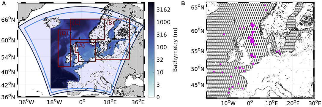
Figure 1. Bathymetry of the wave model WAM (shaded) and domain of the CCLM regional climate model (dark blue box). The area between the dark and light blue boxes is regarded as the buffer zone and is neglected in the analysis. The four different study areas are indicated by the gray boxes in (A) the North Sea (A), the Baltic Sea (B), the southern Norwegian Sea (C), and the North Atlantic Ocean west of the British Isles (D). The locations of the GTS (magenta dots) and Sentinel-3A measurements (gray lines) are shown in (B).

The wave model utilized in this study is the third-generation WAve Model WAM (WAMDI Group, 1988; ECMWF, 2019). WAM has also been used successfully in several studies that assessed the wave-atmosphere coupling together with CCLM (e.g., Cavaleri et al., 2012b; Wahle et al., 2017; Li et al., 2020). However, WAM has also been employed with other atmospheric models, such as the ECMWF model (e.g., Janssen and Viterbo, 1996; Janssen et al., 2002) or the Weather Research and Forecasting (WRF) model (e.g., Wu et al., 2017). WAM is a spectral wave model (WAMDI Group, 1988; ECMWF, 2019) that includes parameterizations for shallow water, depth refraction and wave breaking, making it applicable for the area studied herein. The 2-D wave spectra are calculated on a polar grid with 24 directional 15° sectors and 30 frequencies logarithmically spaced from 0.042 to 0.66 Hz. For the spatial dimensions, a spherical grid is used with a 0.06° longitudinal resolution and a 0.03° latitudinal resolution. The domain of the wave model covers the Baltic and North Seas and the Northeast Atlantic Ocean. The model domain and bathymetry are shown in Figure 1A. At the open boundaries of the model domain, the forcing values come from simulations with a coarser model covering the whole North Atlantic driven by ECMWF Reanalysis Version 5 (ERA5) winds (Copernicus Climate Change Service, 2017). The coarser model has a spatial resolution of 0.25° in both directions and the same spectral resolution as the finer model described above.

These two models are coupled through the OASIS3-Model Coupling Toolkit (MCT) version 2.0 with a coupling time step of 300 s. In the reference simulation, CCLM sends the 10 m wind components to WAM and applies its own parameterization to calculate the roughness length over the ocean using the Charnock formula (Doms et al., 2013), and therefore, the roughness length is dependent only on wind:

$\begin{array}{ll}{z}_0=\frac{{\alpha }_c}{g}max(u_{*}^2,w_{*}^2)& (1)\end{array}$

In Equation 1, the Charnock constant α_c is set to 0.0123, g denotes the acceleration due to gravity, u_* is the friction velocity, and w_* is the scaling velocity for free convection. The roughness length over ice is set to a constant value of 0.001 m.

In the coupled simulation, WAM still receives the wind components but also sends the roughness length calculated through the wave parameters to the atmospheric model. Hence, over the ocean surface, waves are taken into account when estimating the roughness length by using the wave-induced stress (τ_w) for the calculation of z₀.

$\begin{array}{ll}{z}_0=\frac{\widehat{\alpha }\tau }{g}\frac{1}{\sqrt{1-\frac{\tau }{{\tau }_w}}}& (2)\end{array}$

The total stress ($\tau =u_{*}^2$), the acceleration due to gravity (g) and the modified Charnock constant ($\widehat{\alpha }=0.01$) are also taken to calculate the roughness length over the ocean.

2.2. Experimental Design

To analyse the internal variability of the atmospheric model in comparison with the internal variability of the coupled model system and the effects of the wave-atmosphere coupling on the atmospheric model, six different ensemble simulations are carried out and described in Table 1. The ensembles are designed such that there is always a corresponding reference and coupled simulation. The basic set of ensembles is conducted using ERA5 boundary conditions (Copernicus Climate Change Service, 2017), and no spectral nudging is applied in CCLM to allow the atmospheric model to freely develop and to estimate the impacts of coupling on the freely evolving atmosphere. Furthermore, two sensitivity experiments are carried out: one set of ensembles is conducted with spectral nudging, and another set of ensembles is performed using different boundary conditions. Spectral nudging is used to ensure that the large-scale circulation and positions of low-pressure systems are approximately correct using coarser global data, such as reanalyses (von Storch et al., 2000; Weisse and Feser, 2003). For the simulations with spectral nudging, boundary values for the open lateral boundaries as well as for spectral nudging are taken from ERA5 (Copernicus Climate Change Service, 2017) similar to simulations without spectral nudging. To estimate the sensitivity of coupling to the choice of boundary conditions and to assess the impacts of the boundary conditions of the atmospheric model on the effects of the coupling, one set of ensembles is performed using ERA-Interim as boundary conditions (Berrisford et al., 2009; Dee et al., 2011).

TABLE 1

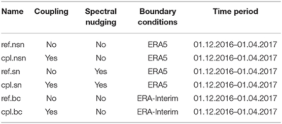
Table 1. Experimental design.

In the atmospheric model, the soil moisture content needs time to adapt (Geyer, 2014). This adaptation occurs faster closer to the surface than for deeper soil layers and depends both on the accuracy of the initial conditions and on the regional conditions. Considering the model domain and that the evaluation of the results is performed mainly for ocean areas, 1 year of spin up is performed starting on 1 January 2016. This spin-up simulation is conducted with the reference set-up involving spectral nudging, which is initialized with ERA5 data. The ensemble initialization is accomplished following Ho-Hagemann et al. (2020) using different dates. Other studies have adopted a similar approach to assess the internal variability of atmospheric models (Alexandru et al., 2007; Lucas-Picher et al., 2008; Sieck, 2013). Lucas-Picher et al. (2008) further assessed other ways to disturb the initial ensemble conditions and found that neither the source nor the magnitude of the perturbations of initial conditions has an impact on the internal variability 15 days past the initialization. Like in Sieck (2013), each experiment consists of 10 ensemble members using restart fields from 1 to 10 December 2016 from the spin-up simulation, as Alexandru et al. (2009) showed 10 members are required for a robust estimate of the internal variability. All restart fields are then used to initiate the ensemble on 1 December 2016, which spans one winter season until 1 April 2017. For the study period the month of december is then dicarded as a spin up for the ensemble. This period is chosen to account for the effects of coupling, especially during extreme events that occur during this time of the year (Janssen et al., 2002; Wahle et al., 2017; Wu et al., 2017; Wiese et al., 2019).

2.3. Observations

2.3.1. In situ Measurements

Observations from the Global Telecommunication System (GTS) of the significant wave height and wind speed are used to estimate the agreement between the model simulations and observations. The data are obtained from and archived at ECMWF (Bidlot and Holt, 2006). Moreover, data are gathered by ECMWF as part of the Joint Technical Commission for Oceanography and Marine Meteorology (JCOMM) wave forecast verification project (Bidlot et al., 2002). The data are recorded either by moored wave buoys anchored at fixed locations to serve national forecasting needs or by instruments mounted on platforms or rigs managed by the oil and gas industry. As in Wiese et al. (2018), the wave height measurements are collocated with the model data using the closest grid point to the location of the in situ observations. The wind speed measurements are interpolated to a height of 10 m above the surface and then collocated with the model using the closest grid point to the location of the observation. The locations of in situ observations are presented in Figure 1B.

2.3.2. Satellite Data

The significant wave height and wind speed observations from the Sentinel-3A satellite are used to assess the realism of the simulated wave characteristics. Sentinel-3A, which was launched in February 2016, is the first altimeter to operate entirely in synthetic aperture radar (SAR) mode (ESA, 2015). The revisit time of Sentinel-3A is 27 days. The data gathered by Sentinel-3A are retrieved from 1D profiles along the ground track of the satellite, and the footprint size is between 1.5 and 10 km depending on the sea state across the track. The along-track resolution of Sentinel-3A is ~7 km for 1 Hz measurements. Figure 1B shows the locations of the satellite measurements. The satellite data are collocated with the model using the nearest model grid point and the closest time with a maximum time lag of 30 min. The in-situ and Sentinel-3A observational data are also described in Wiese et al. (2019).

3. Impacts of the Wave-Atmosphere Coupling

Wind is directly influenced by the coupling through changes in the roughness length that alter the wind speed and direction. Furthermore, the roughness length impacts the MSLP since the roughness determines the angle of wind with respect to the isobars and therefore drives the mass transport from higher to lower pressures (Janssen, 2004). Hence, hourly outputs of wind speed and the MSLP are chosen for more detailed analyses in the following.

In addition, the effects of the internal variability in the atmospheric model and the impacts of coupling on the significant wave height are analysed. For these analyses, four regions are chosen with different wave conditions and storm activity characteristics: the North Sea (A), the Baltic Sea (B), the southern Norwegian Sea (C), and the North Atlantic Ocean west of the British Isles (D). The Baltic Sea exhibits only a very small opening to the North Sea through the Danish Straits and is therefore classified as a closed area for waves. As a result, the fetch conditions are limited within the Baltic Sea, especially in the longitudinal direction. The North Sea is open to the Atlantic Ocean through the English Channel, and swells stemming from the North Atlantic regularly enter the North Sea from the northern opening between Scotland and Norway. The Norwegian Sea and the North Atlantic west of Great Britain are exposed to large swells and long fetch conditions, which are conducive to the development of large waves.

3.1. Differences Between Coupled and Reference Ensembles

The average synoptic situation of ref.nsn during the whole study period and the differences between ref.nsn and cpl.nsn are analysed. For this, the mean values over the ensemble members and over the whole study period of ref.nsn along with the differences between the mean values over the ensemble members and the study period of cpl.nsn and ref.nsn are depicted (Figures 2A,C,E,G). In general, over the entire study period, an increase in the roughness length leads to decreases in the wind speed, significant wave height and pressure gradient. Moreover, while the effects of the coupling on the wind speed and roughness length are limited to the domain coupled to the wave model, changes in the MSLP and geopotential height extend over the whole atmospheric model domain, outside the coupled area and over the European continent.

FIGURE 2

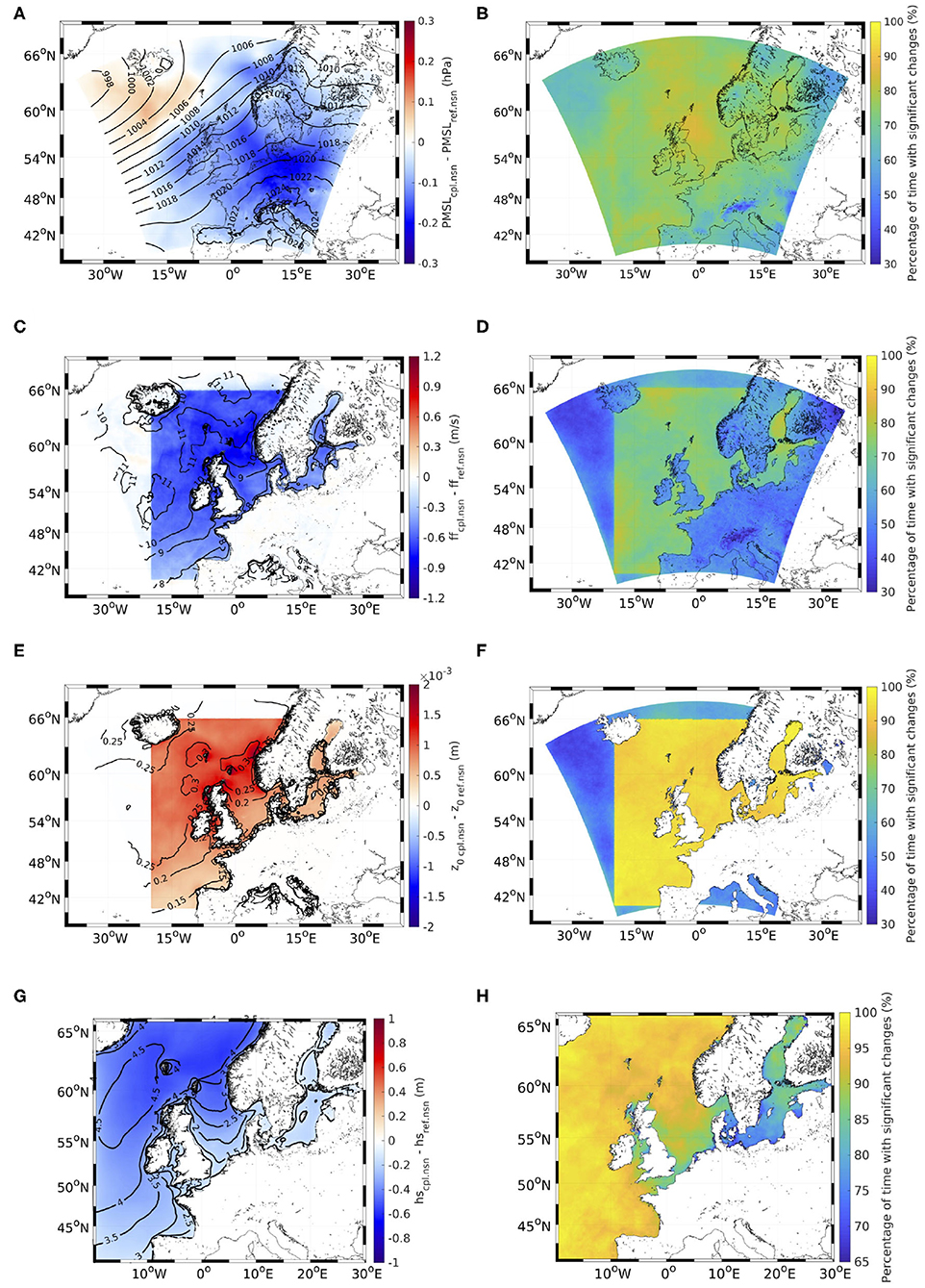
Figure 2. Mean values over 3 months of the MSLP (A), wind speed (C), roughness length (E), and significant wave height (G). The contours reflect the values of the reference simulation, while the colors represent the difference between the coupled (cpl.nsn) and reference (ref.nsn) ensembles for the ensembles without spectral nudging. The percentage of time with significant differences between the coupled and reference ensembles in the MSLP (B), wind speed (D), roughness length (F), and significant wave height (H) are also shown [Note the different color bar range for (H)].

The mean MSLP conditions are characterized by lower pressures west of Iceland and higher pressures over southern Europe. However, due to the wave-atmosphere coupling, this pressure gradient is slightly reduced (Figure 2A). This reduction can be traced directly to the enhancement of the roughness length (Figure 2E) since the surface roughness determines the ageostrophic wind component, responsible for cross-isobar mass transport. This corresponds to the results found by Lionello et al. (1998), Janssen et al. (2002), and Wu et al. (2017). Additionally, the wind speed at 10 m is reduced over the coupled ocean surface (Figure 2C), which can also be attributed directly to the enhanced surface roughness (Figure 2E). This similarly corresponds to several previous studies (e.g., Doyle, 1995; Lionello et al., 1998; Wahle et al., 2017). While the MSLP changes spread over the whole model area, the effect of the reduced wind speed is mostly limited to the coupled model area. The significant wave height is accordingly reduced with the wind speed (Figure 2G). The largest reduction is observed between Norway, Great Britain and Iceland. In this area, the significant wave height, wind speed and roughness length in the reference simulation are the largest, and consequently, the roughness length is considerably enhanced, which results in the largest wind speed and the greatest significant wave height reduction. Smaller reductions in wind speed occur in the Bay of Biscay, the southeastern North Sea and the Baltic Sea, especially in the northern and southern Baltic Sea. The largest part of these small wind speed reductions can be traced to the weaker winds and smaller significant wave heights in those areas, leading to smaller roughness lengths and therefore smaller reductions in wind speed. This leads to a pattern featuring the whole southern North Sea having a relatively small reduction in wind speed, but along the British coast, the reduction in wind speed is larger than in the rest of the North Sea. Moreover, the impacts of the coupling extend further upwards. At 850 hPa, the change in geopotential displays a similar pattern as the change in MSLP with a reduction over the European continent and an increase between Iceland and Scotland (Supplementary Figure 1A). This pattern leads to a reduced geopotential gradient since the geopotential is higher over the southeastern part of the model domain and lower over the northwestern part. At a height of 500 hPa, this pattern is still visible, but the increase in the geopotential between Iceland and Scotland is larger than the decrease over the continent (Supplementary Figure 1C), which is contrary to the changes in the 850 hPa geopotential and MSLP. Nevertheless, this pattern can be interpreted as a reduction in the geopotential gradient at 500 hPa.

Ensemble simulations are conducted with the aim of making conclusions about the significance of differences between the coupled and reference simulations in comparison with the internal variability of the models. This is carried out in order to distinguish whether the coupling has a significant effect on the atmosphere or the impacts are within the range of internal variability of the atmospheric model. To ascertain the significance of these changes, for each grid cell and time step, it is determined whether cpl.nsn and ref.nsn differ significantly from each other using a t-test with a significance interval of 95% (Janssen and Viterbo, 1996; Weisse et al., 2000). With the results of the t-test for each grid cell and time step, the percentage of time in each grid cell where cpl.nsn and ref.nsn differ significantly from one another is calculated, and the results are shown in Figures 2B,D,F,H. For the results presented in Table 2, the mean values over the different areas are calculated. This analysis reveals that cpl.nsn and ref.nsn differ significantly during the majority of the study period not only for parameters close to the surface but also for parameters in higher parts of the atmosphere.

TABLE 2

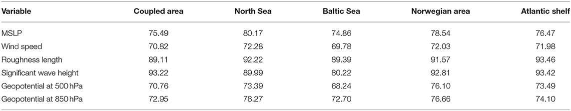
Table 2. Time with significant differences between the coupled (cpl.nsn) and reference (ref.nsn) ensembles (%).

The enhancement of the roughness length is significant 89% of the time within the whole coupled area (Figure 2F and Table 2). This is also the case for the Baltic Sea, whereas in the North Sea, the Norwegian Sea and the North Atlantic Shelf, the changes are significant more than 90% of the time. Regarding the wind speed, the differences between ref.nsn and cpl.nsn are significant 71% of the time within the whole coupled area (Figure 2D). Again, the Baltic Sea has the lowest value with just under 70%, while the other three areas have significant changes in wind speed due to the coupling for ~72% of the study period. For the roughness length and wind speed, the significance of changes decline outside the coupled area, while for the MSLP, significant changes are observed over the entire model area (Figure 2B). In the case of the MSLP, the changes due to coupling are significant 75% of the time within the whole coupled area. As before, the Baltic Sea has the smallest value with 74.86% out of the four areas analysed, while the North Sea has the largest value with significant changes 80.17% of the time due to the coupling. The percentages of time in the Norwegian Sea and the North Atlantic west of the British Isles range between the values in the Baltic and North Sea.

The changes in significant wave height are significant 93% of the time within the whole model area (Figure 2H). In the Baltic Sea, this percentage is reduced to 80.22%, and in contrast to the other parameters, the North Sea has lower values than those elsewhere with significant changes almost 90% of the time. For the Norwegian Sea and the North Atlantic Shelf, which are more exposed to higher significant wave heights and larger changes, the changes are significant for ~93% of the study period.

The coupling also has significant impacts higher in the atmosphere. At 850 hPa, the changes are significant 73% of the time (Supplementary Figure 1B). The changes are significant for the most time within the North Sea region and for the least amount of time in the Baltic Sea, whereas the other two areas have values between those in the North and Baltic Seas. The time with significant differences between cpl.nsn and ref.nsn reduces with increasing height. At 500 hPa, the time characterized by significant differences averaged over the whole coupled area is 70.76% (Supplementary Figure 1D). The longest percentage of time with significant changes is detected in the Norwegian Sea at 76.1%, while the percentages in the North Sea and the North Atlantic Shelf are 73.39 and 73.49%, respectively. The shortest amount of time with significant changes is again found in the Baltic Sea at 68.25%. Hence, it can be concluded changes in roughness length still lead to significant changes higher in the atmosphere.

3.1.1. Probability of Ensemble Differences

Figure 3 shows histograms of the probability of differences between ref.nsn and the cpl.nsn for the four study areas over the whole study period. In general, the wind speed is reduced in cpl.nsn compared to ref.nsn since energy is needed for wave growth. These strengthened waves subsequently enhance the surface roughness, which leads to a reduction in wind speed. However, the magnitude of this reduction varies among the four areas.

FIGURE 3

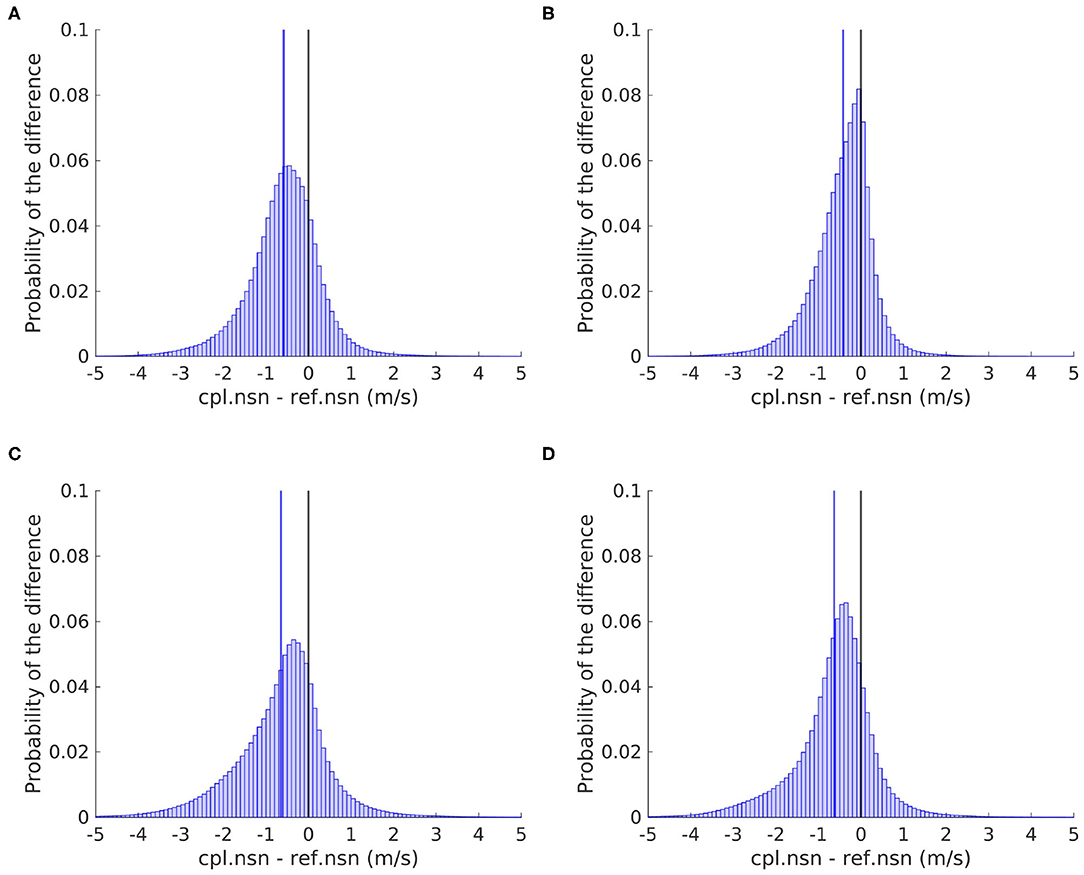
Figure 3. Histogram of the difference in the wind speed between the coupled (cpl.nsn) and reference (ref.nsn) ensembles within the North Sea (A), the Baltic Sea (B), the southern Norwegian Sea (C), and the North Atlantic Ocean west of the British Isles (D). The blue line indicates the mean of the distribution, and the black indicates the zero line.

The mean reductions in the wind speed within the Norwegian Sea and the North Atlantic Ocean west of the British Isles are very similar with values of −0.64 m/s (Figure 3C) and −0.63 m/s (Figure 3D), respectively. In the North Sea, the mean reduction is −0.58 m/s (Figure 3A), while the Baltic Sea has the smallest mean reduction of −0.42 m/s (Figure 3B). These differences can be explained by the significant wave heights in these areas (Figure 4). The Baltic Sea is a very sheltered area surrounded by coastline on all sides. Therefore, the fetch is very limited, and only swells travelling north-south can become larger. Due to mostly short fetches, the wave field cannot develop fully at higher wind speeds, as the distance to the coast is too short. For a fully developed sea state at a wind speed of 20 m/s, a fetch well exceeding 1,000 km is needed (Komen, 2002), which is far greater than the Baltic Sea can provide in most directions. Therefore, winds provide less energy and momentum to waves, and thus, the waves cannot reach their full height, which results in smaller wind speed reductions. Another aspect of wave growth important for fully developing the sea state is the wind speed and the duration of wind speeds. Full development takes more time for high wind speeds, than low wind speeds. The mean wind speed within the Baltic Sea being smaller than those in the other areas (Figure 2C), contributes further to smaller significant wave heights and hence smaller reductions in the roughness length and wind speeds in the Baltic Sea. The distribution of the significant wave height in the Baltic Sea shows a peak at 0.4 m with 99% of all significant wave heights below 4.2 m (Figure 4B). Since the significant wave heights are small, the roughness length is short. Hence, the wind speed changes are small when small significant wave heights occur. In the North Sea, the significant wave heights are larger than those in the Baltic Sea (Figure 4A). The North Sea is open to the Atlantic Ocean in the north and accesses the Atlantic in the west through the English Channel. Through these openings, especially that in the north, large swells can enter the North Sea. Furthermore, the fetch in the North Sea is larger than that in the Baltic Sea. Since large significant wave heights occur, the impacts of the coupling are larger in the North Sea than in the Baltic Sea. The largest impacts, however, occur in the areas that are truly exposed to the open ocean, such as the Norwegian Sea and the North Atlantic Ocean west of the British Isles. Significant wave heights up to 17.87 m in the reference ensemble and 13.53 m in the coupled ensemble occur. Furthermore, the mean significant wave heights in these areas are much larger at ~4 m compared with values of ~2 and 1 m in the North and Baltic Seas, respectively. Since the Norwegian Sea and the North Atlantic Ocean are subject to the largest significant wave heights (Figure 4), the impact of the coupling is the largest (Figure 3). Due to the corresponding reductions in wind speed, the significant wave heights are reduced in the coupled ensemble in all four areas (Figure 4).

FIGURE 4

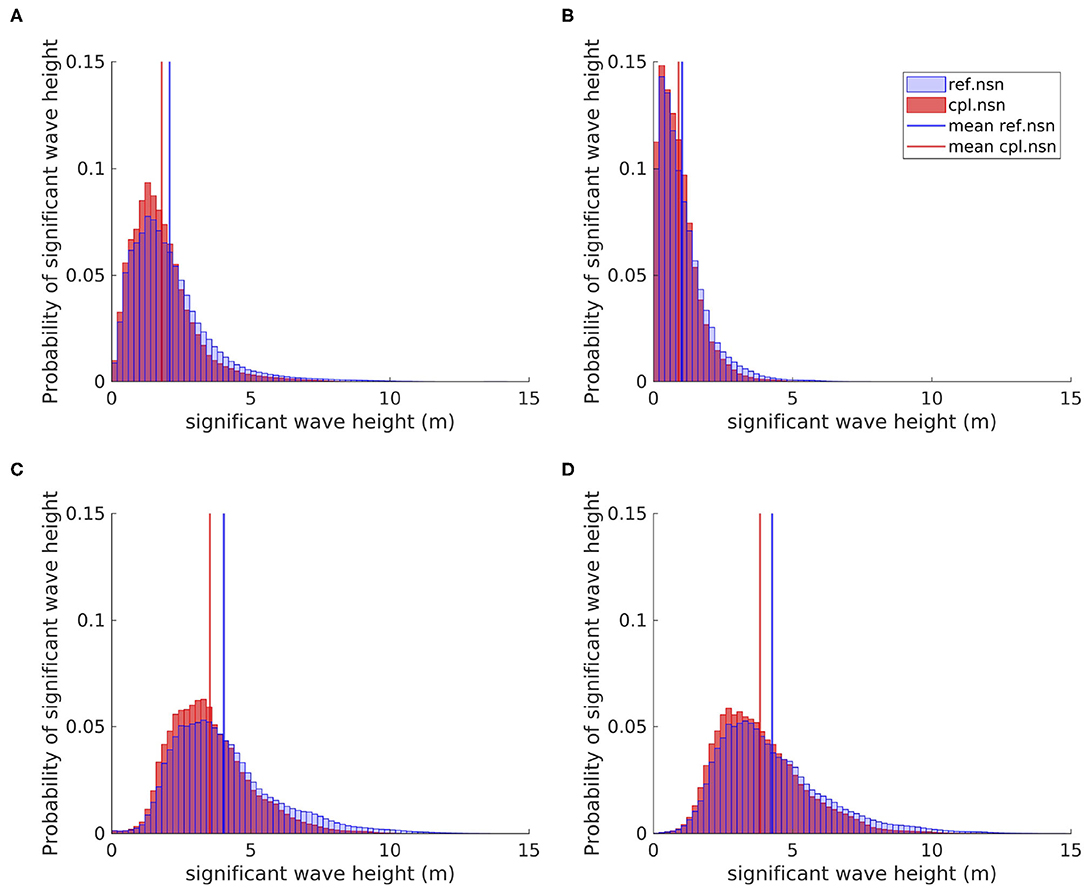
Figure 4. Histogram of the significant wave heights of the reference (ref.nsn) and coupled (cpl.nsn) ensembles within the North Sea (A), the Baltic Sea (B), the southern Norwegian Sea (C), and the North Atlantic Ocean west of the British Isles (D).

The spreads of the distributions of the changes due to the coupling vary among the different areas. The Norwegian Sea and the North Atlantic Ocean west of the British Isles have the largest spreads with values of 1.11 and 1.01 m/s, respectively, since the significant wave heights in these areas similarly show the largest spreads. Small significant wave heights occur during phases with low wind speeds, but very large significant wave heights can be present during stormy periods, when waves are given sufficient time and long fetches to develop. In the North Sea, the spread of the distribution is 0.86 m/s, while that in the Baltic Sea is 0.71 m/s. These small spreads are due to the limited wave growth in these areas due to the fetch and water depth conditions. Thus, the largest significant wave heights in the Norwegian Sea and the North Atlantic Shelf cannot develop in the North and Baltic Seas. Therefore, the spreads of the significant wave height are smaller in the North and Baltic Seas, resulting in smaller distributions of changes in the wind speed. Therefore, the coupling has the largest impacts on the Norwegian Sea and the North Atlantic Ocean west of the British Isles, followed by the North Sea, while the smallest impact is found on the Baltic Sea.

The mean MSLP difference between cpl.nsn and ref.nsn tends toward lower pressures in the coupled ensemble than in the reference ensemble (Figure 5). This trend is the largest in the North Sea and might be related to the geography of the North Sea, which is generally positioned between a low-pressure system moving through the area to the north and a high-pressure system moving over the continent but is more influenced by the reduction in the pressure over the continent (Figure 2A). Since the general change in MSLP constitutes a reduction in the pressure gradient, both reduced and enhanced MSLPs can be found due to the coupling between the wave and atmospheric models in all four areas. In particular, the Norwegian Sea and the North Atlantic Ocean are situated along the border between increasing and decreasing pressure (Figure 2A). This is further reflected in the distribution of the MSLP differences in, where the mean is very close to zero and the distributions are spread similarly in positive and negative sectors (Figures 5C,D). The Baltic Sea is again the least influenced by the coupling (Figure 5B) since the waves are smaller in this area (Figure 4B), influencing the winds less (Figure 3B).

FIGURE 5

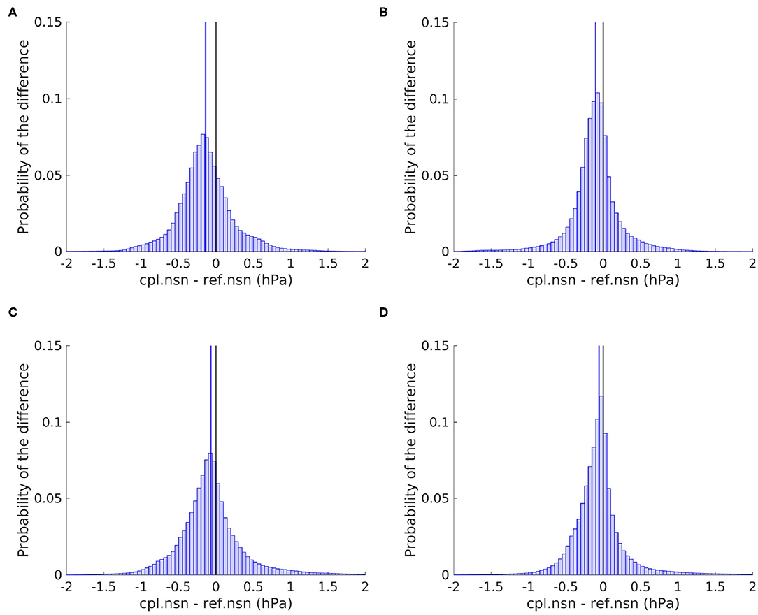
Figure 5. Histogram of the MSLP difference between the coupled (cpl.nsn) and reference (ref.nsn) ensembles within the North Sea (A), the Baltic Sea (B), the southern Norwegian Sea (C), and the North Atlantic Ocean west of the British Isles (D). The blue line indicates the mean of the distribution, and the black indicates the zero line.

3.1.2. Ensemble Spread

The standard deviation (Equation 3) between the ensemble members is regarded as the spread of the ensemble, which is a measure for the internal variability of the system (Ho-Hagemann et al., 2020):

$\begin{array}{ll}Sdt=\sqrt{\frac{1}{N-1}{\displaystyle \sum _{i=1}^N}{(x_i-\overline{x})}^2}& (3)\end{array}$

where {x₁, x₂, x₃, ..., x_N} are the values of each ensemble member for a given variable, $\overline{x}$ represents the mean of the ensemble for the variable and N is the number of members of the ensemble, which is 10 in this study.

The probabilities of the standard deviation of the ensembles of the 10 m wind speed, MSLP and significant wave height are shown in Figure 6. In general, the ensemble spread in cpl.nsn is smaller than that in ref.nsn, with larger probabilities for small standard deviations and smaller probabilities for larger standard deviations. This change is near the mean standard deviation of both ensembles (vertical lines).

FIGURE 6

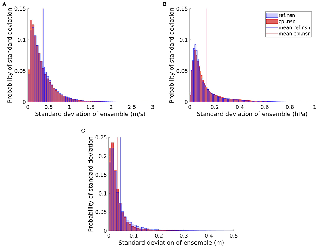
Figure 6. Histogram of the standard deviation of the reference (ref.nsn) and coupled (cpl.nsn) ensembles within the North Sea for the wind speed (A), MSLP (B), and significant wave height (C).

The mean of the standard deviation of wind speed in ref.nsn is 0.37 m/s, and that in cpl.nsn is 0.35 m/s, which constitutes a reduction of 7.46% (Table 3). The reduction in the 99th percentile is 10.53%, but the largest reduction is found in the maximum of the ensemble spread with 23.48%. This shows that the spread in cpl.nsn is generally smaller than that in ref.nsn. Hence, due to the reduction in internal variability, the uncertainty in the coupled system is reduced compared to the reference model.

TABLE 3

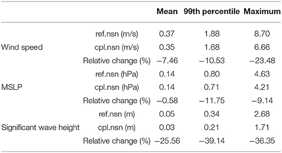
Table 3. Evaluation of ensemble spread.

The MSLP spread in the ensembles is generally quite low (Figure 6B) with a mean of ~0.14 hPa (Table 3). The maximum spread is reduced by 9.14% due to the wave-atmosphere coupling. Therefore, although the internal MSLP variability of the ensembles is already very low, the maximum internal variability can still be reduced due to the coupling.

The variability of the significant wave height due to the wind speed variability is generally quite low at 5 cm in the reference ensemble and 3 cm in the coupled ensemble (Figure 6C and Table 3). The maximum spread, however, can be quite large (up to 2.68 m in the reference simulation). This spread is considerably reduced by 36.35% to 1.71 m due to the coupling and the related reduction in the wind speed uncertainty within the atmospheric model (Figure 6A and Table 3).

In summary, coupling the wave model to the atmospheric model reduces the ensemble spread and therefore also the internal variability of the atmospheric model. In addition, the wave model profits from the reduction in wind speed variability with less variability of the significant wave height.

3.2. Temporal Evolution

After generally assessing the impacts of the wave-atmosphere coupling in comparison with the internal variability of the atmospheric model, a temporal analysis is performed. Figure 7 presents the average wind speed, MSLP and significant wave height in the reference ensemble within the North Sea, which is the area the main analysis is conducted for. Furthermore, the absolute value of the mean differences between the coupled and reference ensembles are depicted along with the spread of the ensembles. This analysis is conducted in order to estimate under which conditions the spread of the ensembles and, therefore, the internal variability, as well as the effects of the coupling become large. Furthermore, this shows whether the ensemble spread or the effects of the coupling are larger and whether during events with high impacts by the coupling, the influence of the waves on the atmosphere is still larger than the internal variability of the atmospheric model. The analysis generally shows that the differences between cpl.nsn and ref.nsn are larger than the internal variability. Thus, the effects of the coupling can be clearly differentiated from the internal variability of the model. Furthermore, the internal variability is reduced in cpl.nsn compared to ref.nsn, especially when the internal variability is large.

FIGURE 7

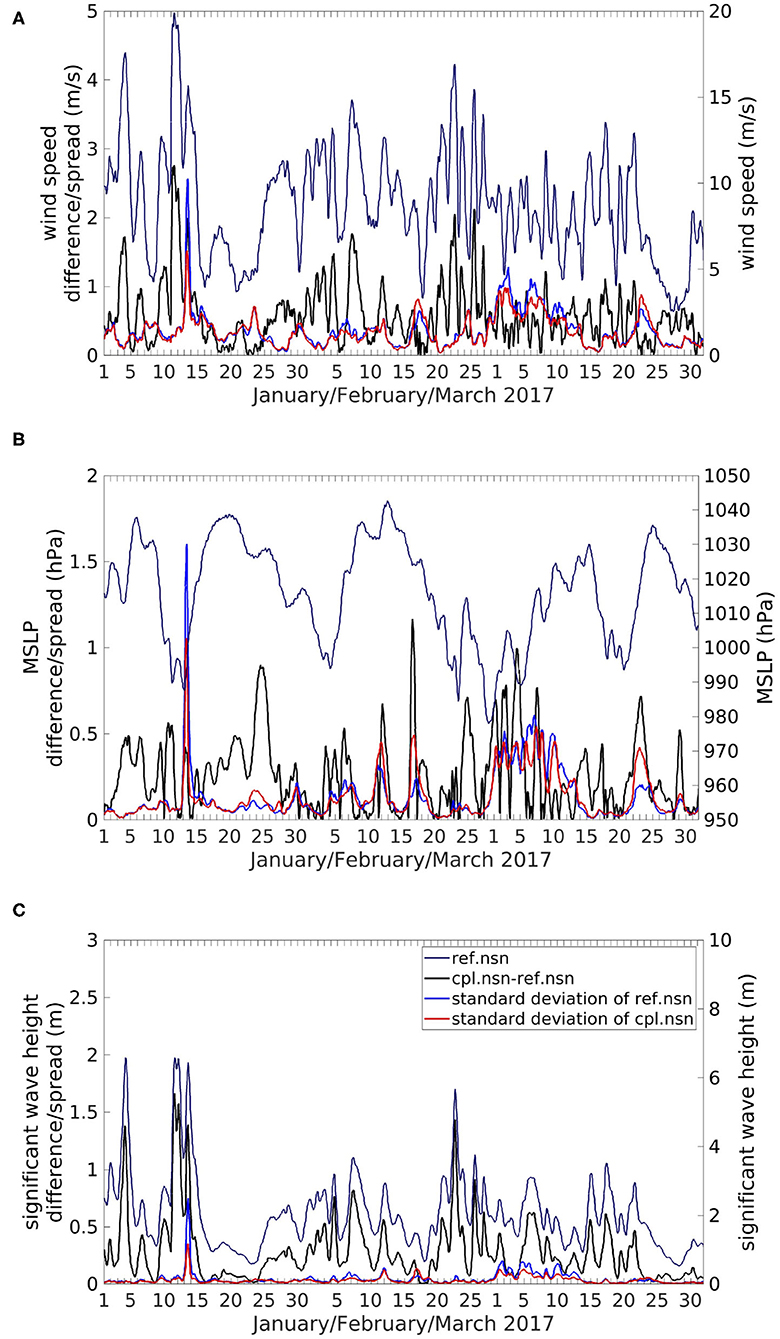
Figure 7. Time series of the absolute differences in the ensemble means (black), standard deviations of the ensembles (red and blue) and values in the reference ensemble (ref.nsn, dark blue, right y-axis) in the North Sea for the wind speed (A), MSLP (B), and significant wave height (C).

A peak in difference between cpl.nsn and ref.nsn can be detected simultaneously with the peak wind speed in ref.nsn (Figure 7A). This indicates that at higher wind speeds, the impact of the coupling between the two models is larger than that at lower wind speeds. At high wind speeds, the sea state needs more time to reach a fully developed state, and before that, the transfer of momentum and energy from the atmosphere to the waves is larger than when the sea state is already fully developed. Moreover, the roughness length is larger for young, developing waves than for old, mature waves, and thus, when the sea state is fully developed, the roughness length becomes smaller, and less energy is transferred from the atmosphere to the waves (Wu et al., 2017). The largest impacts of the coupling on the wind speed and significant wave height appear on 11 January, and the largest internal variability is identified 2 days later. This event is analysed in more detail in section 5.

During the majority of the simulation period, the difference between cpl.nsn and ref.nsn is larger than the internal variability (Figure 7A), which corresponds to significant changes by the coupling ~70% of the time (Figure 2D). This is especially the case when the wind speed is high and when the differences between the coupled and reference ensembles are larger. Therefore, when the coupling has large impacts on the atmosphere by reducing the wind speed, the internal variability is still small, and the differences between the ensemble means can be differentiated from the internal variability of the atmospheric model and traced back as impacts of the coupling. Furthermore, events can occur during which the internal variability becomes larger than the differences between the ensemble means, and as a result, the ensembles cannot be differentiated from one another. Nevertheless, only sporadic events occurred during our study period, whereas the times when the differences between the ensemble means are larger than the ensemble spread are dominant. Furthermore, during events with large internal variability, the uncertainty is reduced in cpl.nsn compared to ref.nsn, which is in accordance with the results of Figure 6.

Since the initial and boundary conditions and the wave model set-up are identical for all simulations, the variability of the wave model is attributable to the different winds in the atmospheric model initiated with different initial conditions. The variability in the wave model, however, is very small most of the time (Figure 7C). Only in very few events is the variability of the significant wave height increased, which is due to an increase in the wind speed variability within the atmospheric model. Therefore, when the internal variability for wind speed is reduced due to the coupling, the variability of the significant wave height is reduced as well. The differences in the significant wave height between cpl.nsn and ref.nsn follow the curve of the significant wave height in ref.nsn in the area. This indicates that the coupling impacts are larger for situations with large significant wave heights and smaller for situations with small significant wave heights. The impacts of the coupling in this case can be very clearly differentiated from the variability of the significant wave height, which is in accordance withthe differences between ref.nsn and cpl.nsn being significant 93% of the time (Figure 2H).

Examining the MSLP time series reveals a similar scenario (Figure 7B). Here, like for the wind speed and significant wave height, the differences between cpl.nsn and ref.nsn are larger than the internal variability of the ensembles most of the time and can be differentiated from one another, especially when large differences between the two ensembles are present, even though events can occur during which the internal variability and the ensemble difference have the same magnitude or the internal variability is larger than the differences. In addition, although events sometimes occur where the internal variability is increased in cpl.nsn compared to ref.nsn, during events with large internal variability of the MSLP, the uncertainty is smaller in cpl.nsn than in ref.nsn. Furthermore, the peaks of differences between cpl.nsn and ref.nsn are not always correlated with significant wave height peaks and hence changes in the roughness length (e.g., on 25 January 2017 and 30 March 2017). Therefore, the wave-atmosphere coupling can have impacts on the MSLP that are not directly linked to the change in the roughness length at that location and time, but are due to lasting effects of the coupling on the atmosphere. The findings for the North Sea exist in the other three study areas in a similar way (Supplementary Figures 3–5).

While the main effects of the coupling on the wind speed and the significant wave height are reductions, for the MSLP, increases are also common. The method used here takes the absolute value of the mean of the difference among the areas of interest. Therefore, increases and decreases cancel each other out, which constitutes a conservative approach to assessing the magnitudes of the differences between the ensembles. Another approach was tested in which the mean of the absolute differences among the areas and was found to differ only marginally from the approach used herein.

3.3. Comparison With Measurements

To investigate whether the wave-atmosphere coupling improves the realism of the observations, the results of the ensemble simulations are compared with wind speed and significant wave height measurements. In this study, Sentinel-3A satellite measurements are used in conjunction with in situ GTS station measurements. The combination of satellite and in situ data is highly complementary since the satellite data have good spatial coverage and the in situ data possess good temporal coverage. The general agreement between the measurements and the ensemble means is good but can still be improved with the wave-atmosphere coupling (Figure 8).

FIGURE 8

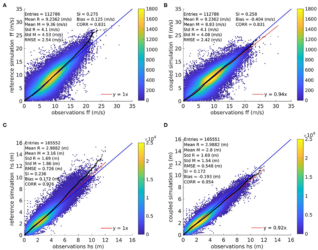
Figure 8. Q-Q scatter plots for the measured (Sentinel-3A and GTS) (reference, R) and modelled (M) wind speeds (A,B) and significant wave heights (C,D) with the reference (ref.nsn) (A,C) and coupled (cpl.nsn) (B,D) ensemble model simulations. The Q-Q plot is shown as black crosses, the 45° reference line is denoted by the blue line, and the least-squares best-fit line is the red line. The equations for the statistical values are provided in the Supplementary Material.

Especially for wind speeds below 7 m/s, the results of both ensembles are very similar to the observations (Figures 8A,B). Beyond that, however, differences begin to show. As in the times series, the most obvious differences between cpl.nsn and ref.nsn can be detected in high wind speed areas. The wind speed in cpl.nsn is reduced compared to that in ref.nsn, which leads to better agreement with the observations. By taking the wave effects on the roughness length into account, the realism of the model simulations is enhanced. The parameterization of the roughness length in the atmospheric model accounting for only the wind speed neglects the variety of wave states and development phases of the sea state at similar wind speeds, which the wave model can depict (Wu et al., 2017). This weakness of the atmospheric model becomes more apparent at higher wind speeds. Thus, the coupling leads to an improved realism of the atmospheric model. This weakness can likewise be detected in comparisons between the measurements and ensemble means of the significant wave height (Figures 8C,D). These differences begin to appear for significant wave heights above 2 m and are especially large for extreme significant wave heights. Although cpl.nsn tends to slightly underestimate large significant wave heights, the agreement between the measurements and cpl.nsn is better than the agreement between the observations and ref.nsn. Mainly the scatter index (Supplementary Equation 5) in significant wave height can be reduced in the coupled ensemble compared to the reference ensemble by 6.4%, hence, increasing the correlation (CORR, Supplementary Equation 7) by 2.8% indicating, that the scatter in the comparison between observed and modelled significant wave height is decreased. Furthermore, the root-mean-square error (RMSE, Supplementary Equation 4) is reduced in the coupled ensemble by 18 cm compared to the reference ensemble. This is to some degree also visible in the wind speed with a reduction of the SI of 1.7% and RMSE of 0.12 m/s.

4. Sensitivity of Coupling to the Application of Spectral Nudging and Different Boundary Conditions in CCLM

4.1. Sensitivity to Spectral Nudging

In the atmospheric model, spectral nudging can be enabled to keep the large-scale atmospheric state close to the forcing data, while regional-scale details are permitted to develop conditioned by the large scales. This method is used for regional and local reconstructions or impact studies, where the representation of the exact weather situation is vital. Furthermore, this method suppresses the internal variability of regional models (von Storch et al., 2000; Weisse and Feser, 2003; Schaaf et al., 2017). Therefore, simulations with spectral nudging are usually reliably closer to observations than those without spectral nudging. On the other hand, this approach might suppress the effects of the coupling (Ho-Hagemann et al., 2020). As shown in the previous section 3, the wave-atmosphere coupling has a positive effect on freely evolving regional models forced only at the lateral boundaries. In this section, it is investigated whether these effects can also be detected in simulations using spectral nudging in the atmospheric model. Hence, we perform a comparison between the effects of the coupling with and without spectral nudging enabled in the atmospheric model. This comparison is conducted mainly for the North Sea. The results show that the coupling has significant impacts on the atmosphere, resulting in better agreement with observations in simulations where spectral nudging is used, with similar impacts of the coupling on the atmosphere as in simulations without spectral nudging.

The wind speed differences in the ensembles with and without spectral nudging are very similar (Figure 9A). The spread of the distribution is smaller for the ensemble with spectral nudging (0.73 m/s) than for the ensemble without spectral nudging (0.86 m/s). This demonstrates that the most extreme coupling effects are smaller in the simulation with spectral nudging, but the general effect is very similar to the effects in the simulation without spectral nudging. For the MSLP, however, this influence is more pronounced than for the other parameters (Figure 9B). Since spectral nudging keeps the larger scales in position, the variability of the MSLP is kept low. Therefore, the coupling tends to reduce the MSLP rather than shift the pressure systems or reduce the pressure gradient.

FIGURE 9

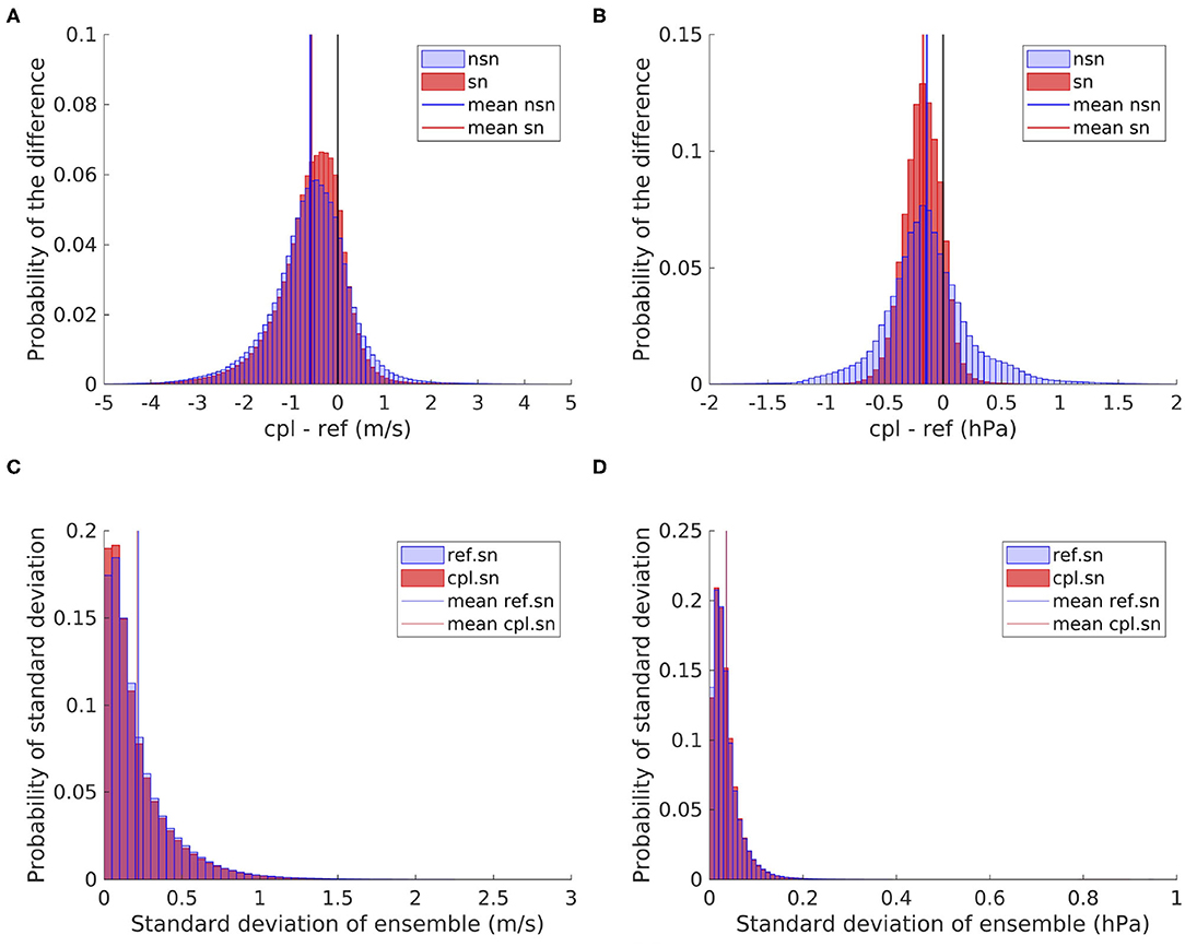
Figure 9. Histogram of the differences between the coupled and reference ensembles in the wind speed (A) and MSLP (B) within the North Sea, as well as the standard deviation of the reference and coupled ensembles within the North Sea area for the wind speed (C) and MSLP (D).

The internal variability is reduced due to spectral nudging (Figures 9C,D) compared to the internal variability of the ensemble without spectral nudging (Figures 6A,B). This has been shown before in several studies (e.g., Weisse and Feser, 2003). The reduction in internal variability due to the coupling, which has been demonstrated in the previous section for simulations without spectral nudging (section 3.1.2), can still be detected in the simulations with spectral nudging (Figures 9C,D and Supplementary Table 1). Therefore, the wave-atmosphere coupling reduces the internal variability even further, which supports the supposition that introducing the wave model reduces the model uncertainty of the atmospheric model.

Weisse and Feser (2003) found that the internal variability appears to be small in ensembles both with and without spectral nudging most of the time and is increased during some periods only in the ensemble without spectral nudging. We detect a similar effect upon examining the time series (Supplementary Figures 2A,C,E). Nevertheless, we discover that the coupling effects on the wind speed (Supplementary Figure 2A) and significant wave height (Supplementary Figure 2E) are almost identical most of the time in simulations with and without spectral nudging. Therefore, although the large scales of the forcing data are kept in the regional model, the coupling of the wave model still influences the wind and wave fields similar to the situation without spectral nudging. Furthermore, as in the simulations without spectral nudging, this coupling leads to better agreement with observations and especially reduces the overestimation of high wind speeds and significant wave heights (Supplementary Figure 6). Hence, coupling the wave model to the atmospheric model enhances the realism of the model simulations also with spectral nudging enabled.

With regard to the impacts of the coupling on the MSLP, the application of spectral nudging in the atmospheric model has a larger impact (Figure 9B; Supplementary Figure 2C). Here, the differences between the coupled and reference ensembles can be differentiated from each other. Most of the time, the impacts of the coupling are very similar, but during events with large differences between cpl.nsn and ref.nsn, these differences become smaller in the simulations with spectral nudging than in those without spectral nudging. Due to spectral nudging, the large-scale atmospheric state is kept close to the forcing data. Hence, the atmosphere has less freedom to develop, and therefore, the coupling impacts on the MSLP are smaller in the simulations with spectral nudging than in those without spectral nudging. Hence, spectral nudging has only a small impact on the effects of the wave-atmosphere coupling on the wind speed and significant wave height, while the effects of the coupling on the MSLP can be suppressed at times.

Furthermore, since the internal variability is reduced due to the inclusion of spectral nudging but the effects of the coupling remain almost identical, the percentage of time with significant changes due to the coupling is increased. The percentage of time that the MSLP is significantly changed is increased from 75.49% in the ensemble without spectral nudging to 87.47% in the ensemble with spectral nudging within the whole coupled model area. The increase in the percentage for the wind speed is ~4–74.89%, and that for the roughness length is ~2.5–91.65%. Additionally, in the higher parts of the atmosphere, the percentages of time with significant changes are similarly increased. The percentage of time with significant changes in the 850 hPa geopotential height increases by more than 10–84.58%, while that in the 500 hPa geopotential height increases by ~9–79.03% within the whole coupled area. Thus, in the ensemble simulations, where spectral nudging is used, the coupling has significant impacts on the atmosphere, resulting in better agreement with observations.

4.2. Sensitivity to Boundary Conditions

The boundary conditions for regional models are usually taken from global models to give realistic values at the lateral boundaries. Here, two different sets of reanalysis data are used as the boundary forcing for the regional model. The boundary conditions can have large impacts on the results of regional model simulations (Déqué et al., 2007; Meißner, 2008; Kjellström et al., 2011; Keuler et al., 2016). Thus, in this study, the impacts of two different boundary conditions, namely, ERA5 and ERA-Interim, in the atmospheric model on the effects of the wave-atmosphere coupling are tested to assess whether the findings in section 3 are robust to different boundary conditions, which is found to be the case.

The general impact of the coupling between the atmospheric model and the wave model is very similar with both boundary conditions, as the distributions of the differences in the wind speed and MSLP are very similar for the ensembles with ERA5 and ERA-Interim boundary conditions (Figures 10A,B). Also the reduction in internal variability is still present with different boundary conditions (Figures 10BC,D). Hence, the effects of the coupling are robust to different reanalysis data used as the boundary forcing (a more detailed analysis can be found in the Supplementary Material).

FIGURE 10

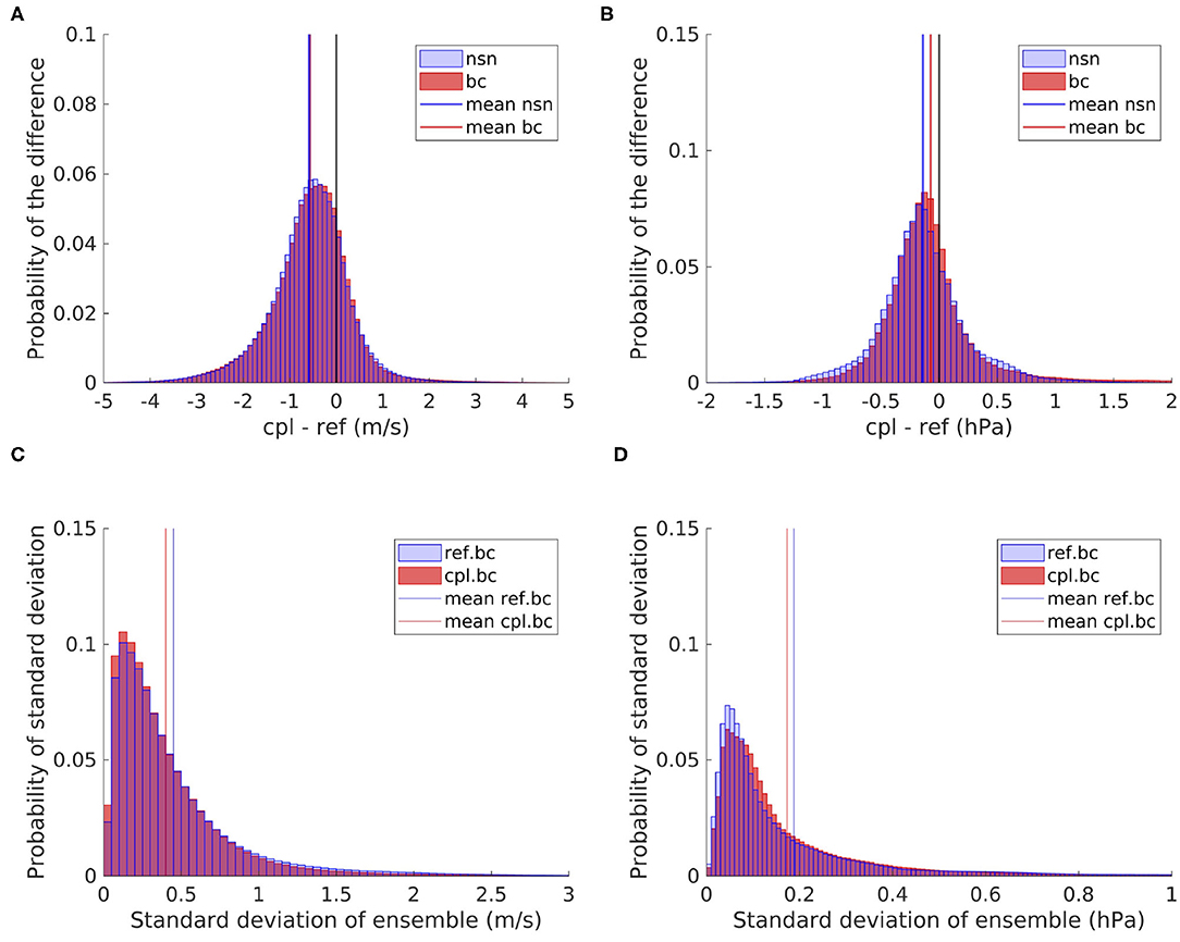
Figure 10. Histogram of the differences between the coupled and reference ensembles in the wind speed (A) and MSLP (B) within the North Sea, as well as the standard deviation of the reference and coupled ensembles within the North Sea area for the wind speed (C) and MSLP (D).

5. Case Study of an Extreme Event

The largest difference in the wind speed and significant wave height between cpl.nsn and ref.nsn is observed on 11 January 2017 (Figure 7A), and the largest internal variability appears 2 days later. Therefore, this event is studied in more detail along with an analysis of the storm tracks of this low-pressure system.

The low-pressure system that passed over the North Sea during mid-January of 2017 formed as a secondary low in the Norwegian Sea. The secondary low was cut off from the main low-pressure system and made its way south across the North Sea, while the core of the main low-pressure system was filled and slowly moved eastwards (Supplementary Figure 8; Figures 11, 12).

FIGURE 11

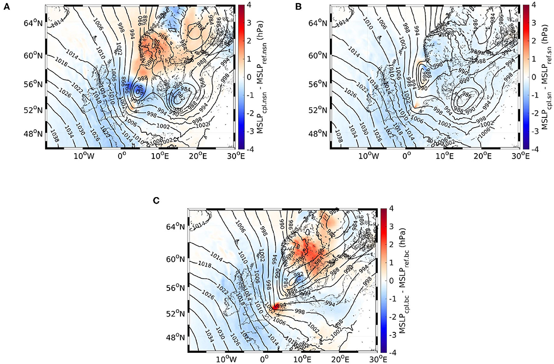
Figure 11. MSLP in the reference simulation on 13 January 2017 at 12 UTC (contour plots) and the differences between the ensemble means of the reference and coupled ensembles both without (A) and with spectral nudging (B), as well as with the changed boundary conditions (C).

FIGURE 12

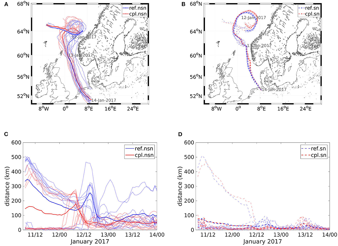
Figure 12. Storm track of the secondary low from 11 January until 14 January 2017 in the simulations without (A) and with spectral nudging (B). Light lines indicate the tracks of individual ensemble members, while the thick lines show the ensemble mean tracks. The distances from the locations of the low of individual ensemble members to the track of the ensemble mean (light lines) and the mean distances of the ensemble members to the ensemble mean (thick lines) in the simulations without (C) and with spectral nudging (D) are also shown.

5.1. Differences in and Variability of the MSLP, Wind Speed, and Significant Wave Height

The largest difference in the wind speed between cpl.nsn and ref.nsn is observed on 11 January 2017 (Figure 7A). At that time, the wind speed is ~20 m/s within the North and Baltic Seas. Since this wind speed is quite high, the reduction in the wind speed is also quite large, transferring energy from the atmosphere to the developing waves. The reduction in wind speed is fairly uniform. The internal variability is very small at that time and only slightly larger in ref.nsn than in cpl.nsn. This is very similar in the ensembles with spectral nudging and the changed boundary conditions (Supplementary Figure 7). Due to the wave-atmosphere coupling, the pressure gradient is reduced at that time in all three ensembles. This reduction in the gradient is due to the enhanced surface roughness, which results in a larger ageostrophic wind component and leads to cross-isobar mass transport from higher to lower pressures. This results in faster filling of the pressure system and hence a reduction in the pressure gradient. This finding is in accordance with previous studies (Lionello et al., 1998; Janssen et al., 2002; Wu et al., 2017). The reduction in the pressure gradient further adds to the reduction in the wind speed. The internal variability of the MSLP is very low in all ensembles, with slightly larger values in the reference ensembles than in the coupled ensembles (Supplementary Figure 8). The reduction in wind speed ultimately leads to a reduced significant wave height. Although the amount of the wind speed reduction is fairly similar within the North and Baltic Seas and in the region between Iceland and Scotland, the decrease in the significant wave height is not uniform. The main attenuation of the significant wave height appears in the areas where the significant wave height peaks in the North Sea and the region between Iceland and Scotland. Since waves have the freedom to develop and are not limited by the fetch or water depth, the energy and momentum from the atmosphere can be converted into wave growth. Furthermore, the reduction in the significant wave height in the Baltic Sea is much smaller than the reductions in the other areas due to fetch limitations. The internal variability of the significant wave height is very low. This scenario is present in all three ensembles, with very slight variations in the magnitude of the difference between the coupled and reference ensembles (Supplementary Figure 9).

The event with the largest internal variability during the study period is observed 2 days later (Figure 7). At that time, the center of the low-pressure system is located directly over the North Sea (Figure 11) with a convergence zone extending from the center of the low-pressure system to the British coast and a wind speed front embedded in that extending north-south over the North Sea (Supplementary Figure 10). The overall changes in the MSLP in both ensembles without spectral nudging again reflect a reduction in the pressure gradient (Figures 11A,C), although other variations can also be detected. One of them is, that the location of this convergence zone differs among the ensembles. The internal variability is quite high in ref.nsn but is reduced in cpl.nsn (Supplementary Figures 11D,G). Nevertheless, this large internal variability is concentrated in the center of the secondary low in the North Sea, while the difference between ref.nsn and cpl.nsn spreads out considerably over the whole area. In the ensemble with the ERA-Interim boundary conditions, the internal variability is substantially diminished (Supplementary Figures 11F,I). In the ensemble with spectral nudging, the internal variability of the MSLP is very low (Supplementary Figures 11E,H), but the differences between cpl.sn and ref.sn are slightly different from those between the ensembles without spectral nudging. However, a shift in the location of the convergence zone can still be detected in the ensembles with spectral nudging (Figure 11B), but instead of a reduction in the pressure gradient, the pressure is reduced in the majority of the area. The differences when spectral nudging is enabled are smaller than those when spectral nudging is not enabled. This shows, that the changes in the MSLP are more sensitive toward the pressure field that is present, which differs due to the varying boundary conditions, and the spectral nudging.

In wind speed a similar picture as in MSLP occurs, although the changes due to the coupling are more similar among the three ensembles (Supplementary Figure 10). In all cases, the differences between the coupled and reference ensembles is a slight varying in the position of the front, and a wind speed reduction, especially behind the front. Since in all ensembles the coupling-induced differences are very similar, these differences can be attributed to the wave-atmosphere coupling. Especially in the simulations with spectral nudging, the differences are much larger than the internal variability, which implies that the differences are the effect of the coupling between the two models. As in MSLP the internal variability can be reduced in the coupled simulations. The effect of the reduction in the wind speed is directly evident in the significant wave height (Supplementary Figure 12). In the North Sea west of the front, the significant wave height is reduced according to the reduction in wind speed. This effect is very similar in all three ensembles. The weaker reduction in the significant wave height can be explained by the water depth on the Dogger Bank (Figure 1). Since the waves can reach only a certain height before breaking, the reduction in the significant wave height is lower in that area than elsewhere. Furthermore, the internal variability of the wind speed is transferred straight into the wave model. Therefore, the uncertainty in the wave model is very similar to the uncertainty in the wind speed, although the changes in the significant wave height are always larger than the internal variability.

5.2. Variability of Storm Tracks

Additionally, the tracks of the secondary low across the North Sea are analysed (Figure 12). A track is defined as the path of the minimum MSLP (for example, in Schrum et al., 2003; Wu et al., 2015; Rizza et al., 2018; Ho-Hagemann et al., 2020). The analysis in the present study shows that the variability of storm tracks can be reduced when the wave-atmosphere coupling is enabled.

The low forms as a secondary low of the low-pressure system situated off the Norwegian coast. In most ensemble members, the low circles around the center of the main low before cutting off and making its way south across the North Sea (Figure 12A). The uncertainty in the exact position of the center of the low is most pronounced during the formation of the secondary low until it starts to move southwards. Furthermore, the distances from the tracks of individual ensemble members to the track of the ensemble mean are the largest during the formation stage (Figure 12C). On 12 January at approximately noon, the low starts to makes its way south across the North Sea. In the area of the Norwegian Sea, the spread of cpl.nsn is reduced compared to ref.nsn, with the tracks becoming more confined farther to the west. The distances from the tracks to the mean ensemble track drop in cpl.nsn as soon as the low is formed and starts moving south on 12 January at noon. The distances remain small for the remainder of the time the low travels across the North Sea. In ref.nsn, however, the tracks spread over the whole North Sea, with larger distances to the mean track. This further illustrates that the coupling reduces the spread in the simulations.

For the simulations where spectral nudging is enabled, the tracks of one ensemble are very close together, which is eventually the goal of using spectral nudging. Nevertheless, variations between ref.sn and cpl.sn can be detected (Figure 12B). One difference is the path of the low is during the formation stage, when the secondary low circles around the center of the main low-pressure system. This is also the area with the largest uncertainty, as the distances from individual ensemble tracks to the track of the ensemble mean are the largest (Figure 12D) since one ensemble member in each ensemble takes a different track during the formation stage. Another difference in the tracks can be detected along the southern tip of Norway. In cpl.sn, the tracks are shifted farther eastwards compared to the tracks of ref.sn. This shift is present in most ensemble members, not only in the ensemble mean. In the Norwegian Sea, where ref.nsn shows large variations, ref.sn also exhibits some variations, albeit much smaller. During that time, the reduction in the variability of the storm track is also visible in the distances from the individual tracks to the ensemble mean. In general, though, the tracks are much closer together in the simulations with spectral nudging, as the distances from individual ensemble members to the mean track are much smaller than in the simulations without spectral nudging. This spread of the storm tracks observed in ref.sn is reduced in cpl.sn, where the path of the low is very similar among all ensemble members.

The above analysis shows that the variability of storm tracks is reduced due to the wave-atmosphere coupling, and spectral nudging reduces the variations in possible storm tracks more than the coupling. However, in simulations with spectral nudging, small changes in storm tracks generated by the coupling are still possible.

6. Summary, Conclusions, and Discussion

From this study on assessing the uncertainties in ensemble simulations with a wave-atmosphere coupled model relative to the impacts of the coupling, it can be concluded that the ensembles of the coupled system and the reference model differ significantly from one another during the majority of the study period but especially during extreme events. Furthermore, the model uncertainty and hence the internal variability can be reduced when using the coupled system compared with a stand-alone atmospheric model. These findings are still valid when using different boundary conditions or spectral nudging in the atmospheric model.

For most of the study period, the reference ensemble differs significantly from the coupled ensemble with regard to surface parameters such as the roughness length, 10 m wind speed, significant wave height and MSLP but also the geopotential heights at 850 and 500 hPa, showing that the signals of waves are transported high into the atmosphere. These differences are especially large during extreme events, while the internal variability usually remains smaller than the impacts of the coupling, particularly in the wind speed and significant wave height. Hence, we can conclude that the effects of the coupling and the internal variability of the atmospheric model in particular can be differentiated when large differences between the coupled and reference ensembles occur. Therefore, we can verify the significant impacts of the wave-atmosphere coupling on the atmosphere for the global ocean found by Janssen and Viterbo (1996) for our regional model set-up.

Moreover, the internal variability of the atmospheric model can be reduced by its coupling to the wave model. This effect can be detected particularly during events where the internal variability increases but is likewise present in the mean over the whole period. These findings are proven robust to the application of different sets of reanalysis data at the lateral boundaries of the atmospheric model.

In addition, one set of ensemble simulations is performed where spectral nudging is enabled in the atmospheric model to test the sensitivity of the coupled system to the implementation of spectral nudging in the atmospheric model. Spectral nudging seems to have almost no influence on the effects of the coupling on the wind speed and significant wave height during the analysed period. The differences in the MSLP, though, can deviate between the simulations without and with spectral nudging for short time periods and are in general smaller for simulations with spectral nudging than for simulations without spectral nudging. In addition, the internal variability is reduced even further due to the coupling.

From this study, it can be concluded that the wave-atmosphere coupling can be advantageous to the operational and climate modelling of waves and atmospheric components. This is especially important for all human activities on the ocean and close to the coast. For marine traffic and the installation and maintenance of offshore energy, precise forecasts are essential. By having significant impacts of the coupling approaching observational data, operational models can clearly benefit from the coupling of wave and atmospheric models, especially during events with high wind speeds. Furthermore, this coupling is also advantageous for regional climate studies. For coastal protection, harbor and offshore energy planning, projections with low uncertainties are needed. The analysis of this winter season showed that the coupling of wave and atmospheric models reduces their uncertainties, and therefore, regional climate studies can profit from this coupling. Since the impacts of the coupling are significant in simulations using spectral nudging in the atmospheric model, in order to keep the large scales closer to the forcing data, for a better local or regional reconstruction, the coupling is recommended to use, especially for the reconstruction of extreme events, where realistic simulation results are desired. With the coupling of the wave model to the atmospheric model, the realism in the atmospheric model is increased and the model uncertainty decreased since the roughness of ocean surfaces depends on the sea state and the development phase of the waves and cannot be sufficiently represented by functions of wind speed only (Wu et al., 2017). This enhanced realism leads to better agreement with observations in the simulations using spectral nudging, as well as in simulations where no spectral nudging is used.

This study highlights the importance of the wave-atmosphere coupling, especially during extreme events, which are greatly important for guaranteeing safety at sea, and thereby emphasizes the importance of utilizing coupled atmosphere-wave models for weather prediction. Another topic to assess in future research is how the impact of this coupling behaves during other seasons of the year. The focus of this study is on the winter months, when the largest impacts of the coupling can be expected due to high storm activity (Janssen et al., 2002; Wahle et al., 2017; Wu et al., 2017; Wiese et al., 2019; Varlas et al., 2020). Furthermore, assessing the model uncertainty stemming from the structure of the model, like grid resolution and altering the model parameters within their range of uncertainty would add to the understanding of uncertainties in the atmospheric model. In the last couple of years, regional climate models have transitioned from stand-alone atmospheric or ocean models to coupled ocean-atmosphere models, thereby adding value to regional climate projections (Schrum, 2017). However, these coupled models rarely incorporate wave models (Schrum, 2017). Therefore, a logical next step for future research would be to integrate a wave model into a coupled ocean-atmosphere model. The benefits of coupling waves with oceanic components have already been shown (Breivik et al., 2015; Staneva et al., 2016a,b). Furthermore, the exchange of heat and mass between the ocean and atmosphere are controlled by the waves (Cavaleri et al., 2012b). Hence, the effects of the waves on these fluxes needs to be investigated in fully coupled atmosphere-waves-ocean systems, since they are highly dependent on all three components of the system. Moreover, Ho-Hagemann et al. (2020) have shown the stabilizing effect of the ocean on the atmosphere. Hence, the effects of coupling all three together on the uncertainty of the system is a point worth to investigate, when using fully coupled models including atmosphere, waves and ocean. With each component added to the coupled system, the depicted processes come closer to the ones occurring in the real earth system, since this interacts on all scales transporting and exchanging energy and momentum. Still, there are approximations in the description of the coupling and other processes within the models, which need further analysis. Therefore, future research on the added value of coupling all three components would be beneficial, as indicated by research on hurricanes (Chen et al., 2007; Warner et al., 2010; Olabarrieta et al., 2012; Zambon et al., 2014; Pant and Prakash, 2020) and offshore energy (Wu et al., 2020). However, further research is needed to assess the interactions among all three components during extratropical storms. The study by Wu et al. (2019) makes for a good starting point for research in this field.

Data Availability Statement

The datasets presented in this article are not readily available because the observational and reanalyses data needs to be requested. The model output can be made available upon request to the corresponding author. Publicly available datasets used in this study can be found from: the ECMWF dataserver (https://apps.ecmwf.int/datasets/) for ERA-Interim data, https://cds.climate.copernicus.eu/cdsapp#!/search?type=application for ERA5 data, https://sentinels.copernicus.eu/documents/247904/1848151/Sentinel-3_Altimetry_Data_Access_and_Products.pdf for Sentinel-3A data.

Author Contributions

AW and JS conceived the work. AW set up the COSMO-CLM, performed all the coupled and reference model simulations, conducted the analyses, and wrote the paper. HTMH-H provided the assistance with the set-up of the COSMO-CLM regional climate model and the initialization of the ensembles. SG and WK implemented the coupling in CCLM and WAM and provided technical support with the model system. CS and JS provided guidance on the overall direction of the work. All authors reviewed the manuscript.

Funding

This publication has received funding from the European Union's H2020 Programme for Research, Technological Development and Demonstration under grant agreement no. H2020-EO-2016-730030-CEASELESS. This work is a contribution to the Excellence Cluster of Universität Hamburg, funded by the DFG under Germany's Excellence Strategy EXC 2037 “Climate, Climatic Change, and Society” Project 390683824. The work described in this article is a contribution to the project “Advanced Earth System Modelling Capacity (ESM)”, financed through the Initiative and Networking Fund of the Helmholtz Association and to the Helmholtz initiative REKLIM.

Conflict of Interest

The authors declare that the research was conducted in the absence of any commercial or financial relationships that could be construed as a potential conflict of interest.

Acknowledgments

The authors would like to thank Jean-Raymond Bidlot from ECMWF for providing the in situ observations, Luciana Fenoglio-Marc from the University of Bonn for making the Sentinel-3A altimeter data available, Arno Behrens for providing the boundary conditions for the wave model, and Ronny Petrik for technical support with CCLM.

Supplementary Material

The Supplementary Material for this article can be found online at: https://www.frontiersin.org/articles/10.3389/fmars.2020.596843/full#supplementary-material

References

Copernicus Climate Change Service (C3S) (2017). ERA5: Fifth Generation of ECMWF Atmospheric Reanalyses of the Global Climate. Available online at: https://cds.climate.copernicus.eu/cdsapp#!/home (accessed July 16, 2020).

Alexandru, A., de Elia, R., and Laprise, R. (2007). Internal variability in regional climate downscaling at the seasonal scale. Mon. Weather Rev. 135, 3221–3238. doi: 10.1175/MWR3456.1

CrossRef Full Text | Google Scholar

Alexandru, A., De Elia, R., Laprise, R., Separovic, L., and Biner, S. (2009). Sensitivity study of regional climate model simulations to large-scale nudging parameters. Mon. Weather Rev. 137, 1666–1686. doi: 10.1175/2008MWR2620.1

CrossRef Full Text | Google Scholar

Bao, J., Wilczak, J., Choi, J., and Kantha, L. (2000). Numerical simulations of air–sea interaction under high wind conditions using a coupled model: a study of hurricane development. Mon. Weather Rev. 128, 2190–2210. doi: 10.1175/1520-0493(2000)128<2190:NSOASI>2.0.CO;2

CrossRef Full Text | Google Scholar

Berrisford, P., Dee, D., Fielding, K., Fuentes, M., Kallberg, P., Kobayashi, S., et al. (2009). The ERA-Interim Archive. Available online at: https://www.ecmwf.int/sites/default/files/elibrary/2011/8174-era-interim-archive-version-20.pdf, (accessed March 01, 2018).

Google Scholar

Bidlot, J., and Holt, M. (2006). Verification of Operational Global and Regional Wave Forecasting Systems Against Measurements From Moored Buoys. Geneva: WMO & IOC.

Google Scholar

Bidlot, J.-R., Holmes, D. J., Wittmann, P. A., Lalbeharry, R., and Chen, H. S. (2002). Intercomparison of the performance of operational ocean wave forecasting systems with buoy data. Weather Forecast. 17, 287–310. doi: 10.1175/1520-0434(2002)017<0287:IOTPOO>2.0.CO;2

CrossRef Full Text | Google Scholar

Breivik, Ø., Mogensen, K., Bidlot, J.-R., Balmaseda, M. A., and Janssen, P. A. (2015). Surface wave effects in the nemo ocean model: forced and coupled experiments. J. Geophys. Res. Oceans 120, 2973–2992. doi: 10.1002/2014JC010565

CrossRef Full Text | Google Scholar

Cavaleri, L., Fox-Kemper, B., and Hemer, M. (2012a). Wind waves in the coupled climate system. Bull. Am. Meteorol. Soc. 93, 1651–1661. doi: 10.1175/BAMS-D-11-00170.1

CrossRef Full Text | Google Scholar

Cavaleri, L., Roland, A., Dutour Sikiric, M., Bertotti, L., and Torrisi, L. (2012b). “On the coupling of COSMO to WAM,” in Proceedings of the ECMWF Workshop on Ocean-Waves (Reading: ECMWF), 25–27.

Google Scholar

Chen, S. S., Price, J. F., Zhao, W., Donelan, M. A., and Walsh, E. J. (2007). The cblast-hurricane program and the next-generation fully coupled atmosphere–wave–ocean models for hurricane research and prediction. Bull. Am. Meteorol. Soc. 88, 311–318. doi: 10.1175/BAMS-88-3-311

CrossRef Full Text | Google Scholar

Chen, S. S., Zhao, W., Donelan, M. A., and Tolman, H. L. (2013). Directional wind–wave coupling in fully coupled atmosphere–wave–ocean models: results from cblast-hurricane. J. Atmos. Sci. 70, 3198–3215. doi: 10.1175/JAS-D-12-0157.1

CrossRef Full Text | Google Scholar

Dee, D. P., Uppala, S., Simmons, A., Berrisford, P., Poli, P., Kobayashi, S., et al. (2011). The ERA-interim reanalysis: configuration and performance of the data assimilation system. Q. J. R. Meteorol. Soc. 137, 553–597. doi: 10.1002/qj.828

CrossRef Full Text | Google Scholar

Déqué, M., Rowell, D., Lüthi, D., Giorgi, F., Christensen, J., Rockel, B., et al. (2007). An intercomparison of regional climate simulations for europe: assessing uncertainties in model projections. Clim. Change 81, 53–70. doi: 10.1007/s10584-006-9228-x

CrossRef Full Text | Google Scholar

Doms, G., and Baldauf, M. (2013). A Description of the Nonhydrostatic Regional COSMO Model. Part I: Dynamics and Numerics. Offenbach: Deutscher Wetterdienst.

Doms, G., Förstner, J., Heise, E., Herzog, H., Mironov, D., Raschendorfer, M., et al. (2013). A Description of the Nonhydrostatic Regional COSMO Model. Part II: Physical Parameterization. Offenbach: Deutscher Wetterdienst.

Donelan, M. A. (2018). On the decrease of the oceanic drag coefficient in high winds. J. Geophys. Res. Oceans 123, 1485–1501. doi: 10.1002/2017JC013394

CrossRef Full Text | Google Scholar

Doyle, J. D. (1995). Coupled ocean wave/atmosphere mesoscale model simulations of cyclogenesis. Tellus A 47, 766–778. doi: 10.1034/j.1600-0870.1995.00119.x

CrossRef Full Text | Google Scholar

ECMWF (2019). Part VII: ECMWF Wave Model. Number 7 in IFS Documentation. Reading: ECMWF.

Google Scholar

ESA (2015). Sentinel-3: Data Access and Products. Available online at: https://sentinels.copernicus.eu/documents/247904/1848151/Sentinel-3_Altimetry_Data_Access_and_Products.pdf (accessed February 5, 2019).

Feser, F., Weisse, R., and von Storch, H. (2001). Multi-decadal atmospheric modeling for europe yields multi-purpose data. EOS Trans. Am. Geophys. Union 82, 305–310. doi: 10.1029/01EO00176

CrossRef Full Text | Google Scholar

Gautier, C., and Caires, S. (2015). “Operational wave forecasts in the southern North Sea,” in 36th IAHR World Congress, 28th June–3 July, Number 1 (The Hague), 2–5.

Google Scholar

Geyer, B. (2014). High-resolution atmospheric reconstruction for Europe 1948–2012: coastDat2. Earth Syst. Sci. Data 6:147. doi: 10.5194/essd-6-147-2014

CrossRef Full Text | Google Scholar

Ho-Hagemann, H. T. M., Gröger, M., Rockel, B., Zahn, M., Geyer, B., and Meier, H. M. (2017). Effects of air-sea coupling over the North Sea and the Baltic Sea on simulated summer precipitation over central Europe. Clim. Dyn. 49, 3851–3876. doi: 10.1007/s00382-017-3546-8

CrossRef Full Text | Google Scholar

Ho-Hagemann, H. T. M., Hagemann, S., Grayek, S., Petrik, R., Rockel, B., Staneva, J., et al. (2020). Internal model variability of the regional coupled system model GCOAST-AHOI. Atmosphere 11:227. doi: 10.3390/atmos11030227

CrossRef Full Text | Google Scholar

Ho-Hagemann, H. T. M., Hagemann, S., and Rockel, B. (2015). On the role of soil moisture in the generation of heavy rainfall during the oder flood event in july 1997. Tellus A 67:28661. doi: 10.3402/tellusa.v67.28661

CrossRef Full Text | Google Scholar

Ho-Hagemann, H. T. M., Rockel, B., Kapitza, H., Geyer, B., and Meyer, E. (2013). COSTRICE: An Atmosphere-Ocean-Sea Ice Model Coupled System Using OASIS3. Geesthacht: Helmholtz-Zentrum Geesthacht.

Google Scholar

Janssen, P. (2004). The Interaction of Ocean Waves and Wind. Cambridge: Cambridge University Press.

Google Scholar

Janssen, P., Doyle, J. D., Bidlot, J., Hansen, B., Isaksen, L., and Viterbo, P. (2002). Impact and feedback of ocean waves on the atmosphere. Adv. Fluid Mech. 33, 155–198. Available online at: https://www.ecmwf.int/sites/default/files/elibrary/2001/10225-impact-and-feedback-ocean-waves-atmosphere.pdf

Google Scholar

Janssen, P. A., and Viterbo, P. (1996). Ocean waves and the atmospheric climate. J. Clim. 9, 1269–1287. doi: 10.1175/1520-0442(1996)009<1269:OWATAC>2.0.CO;2

CrossRef Full Text | Google Scholar

Katsafados, P., Papadopoulos, A., Korres, G., and Varlas, G. (2016). A fully coupled atmosphere-ocean wave modeling system for the Mediterranean Sea: interactions and sensitivity to the resolved scales and mechanisms. Geosci. Model Dev. 9, 161–173. doi: 10.5194/gmd-9-161-2016

CrossRef Full Text | Google Scholar

Kelemen, F. D., Primo, C., Feldmann, H., and Ahrens, B. (2019). Added value of atmosphere-ocean coupling in a century-long regional climate simulation. Atmosphere 10:537. doi: 10.3390/atmos10090537

CrossRef Full Text | Google Scholar

Keuler, K., Radtke, K., Kotlarski, S., and Lüthi, D. (2016). Regional climate change over europe in COSMO-CLM: influence of emission scenario and driving global model. Meteorol. Zeitschr. 25, 121–136. doi: 10.1127/metz/2016/0662

CrossRef Full Text | Google Scholar

Kjellström, E., Nikulin, G., Hansson, U., Strandberg, G., and Ullerstig, A. (2011). 21st century changes in the european climate: uncertainties derived from an ensemble of regional climate model simulations. Tellus A 63, 24–40. doi: 10.1111/j.1600-0870.2010.00475.x

CrossRef Full Text | Google Scholar

Komen, G. J. (2002). “Forecasting wind-driven ocean waves,” in Ocean Forecasting, eds N. Pinardi and J. Woods (Berlin; Heidelberg: Springer), 267–279.

Google Scholar

Laprise, R., Kornic, D., Rapaić, M., Šeparović, L., Leduc, M., Nikiema, O., et al. (2012). “Considerations of domain size and large-scale driving for nested regional climate models: impact on internal variability and ability at developing small-scale details,” in Climate Change, eds A. Berger, F. Mesinger, and D. Sijacki (Vienna: Springer), 181–199.

Google Scholar

Larsén, X. G., Du, J., Bolaños, R., Imberger, M., Kelly, M. C., Badger, M., et al. (2019). Estimation of offshore extreme wind from wind-wave coupled modeling. Wind Energy 22, 1043–1057. doi: 10.1002/we.2339

CrossRef Full Text | Google Scholar

Li, D., Staneva, J., Grayek, S., Behrens, A., Feng, J., and Yin, B. (2020). Skill assessment of an atmosphere–wave regional coupled model over the East China Sea with a focus on typhoons. Atmosphere 11:252. doi: 10.3390/atmos11030252

CrossRef Full Text | Google Scholar

Lionello, P., Malguzzi, P., and Buzzi, A. (1998). Coupling between the atmospheric circulation and the ocean wave field: an idealized case. J. Phys. Oceanogr. 28, 161–177. doi: 10.1175/1520-0485(1998)028<0161:CBTACA>2.0.CO;2

CrossRef Full Text | Google Scholar

Lucas-Picher, P., Caya, D., de Elía, R., and Laprise, R. (2008). Investigation of regional climate models' internal variability with a ten-member ensemble of 10-year simulations over a large domain. Clim. Dyn. 31, 927–940. doi: 10.1007/s00382-008-0384-8

CrossRef Full Text | Google Scholar

Meißner, C. (2008). High-resolution sensitivity studies with the regional climate model COSMO-CLM. Meteorol. Zeitschr. 18, 543–557. doi: 10.1127/0941-2948/2009/0400

CrossRef Full Text | Google Scholar

Murphy, J. M., Sexton, D. M., Barnett, D. N., Jones, G. S., Webb, M. J., Collins, M., et al. (2004). Quantification of modelling uncertainties in a large ensemble of climate change simulations. Nature 430, 768–772. doi: 10.1038/nature02771

PubMed Abstract | CrossRef Full Text | Google Scholar

Olabarrieta, M., Warner, J. C., Armstrong, B., Zambon, J. B., and He, R. (2012). Ocean–atmosphere dynamics during Hurricane Ida and Nor'Ida: an application of the coupled ocean–atmosphere–wave–sediment transport (COAWST) modeling system. Ocean Modell. 43, 112–137. doi: 10.1016/j.ocemod.2011.12.008

CrossRef Full Text | Google Scholar

Pant, V., and Prakash, K. R. (2020). Response of air–sea fluxes and oceanic features to the coupling of ocean–atmosphere–wave during the passage of a tropical cyclone. Pure Appl. Geophys. 177, 3999–4023. doi: 10.1007/s00024-020-02441-z

CrossRef Full Text | Google Scholar

Perrie, W., and Zhang, Y. (2001). A regional climate model coupled to ocean waves: synoptic to multimonthly simulations. J. Geophys. Res. Atmos. 106, 17753–17771. doi: 10.1029/2001JD900207

CrossRef Full Text | Google Scholar

Quante, M., and Colijn, F. (2016). North Sea Region Climate Change Assessment. Springer Nature, xxxix–xlv, 409, 457.

Google Scholar

Rizza, U., Canepa, E., Ricchi, A., Bonaldo, D., Carniel, S., Morichetti, M., et al. (2018). Influence of wave state and sea spray on the roughness length: feedback on medicanes. Atmosphere 9:301. doi: 10.3390/atmos9080301

CrossRef Full Text | Google Scholar

Rockel, B., Will, A., and Hense, A. (2008). The regional climate model COSMO-CLM (CCLM). Meteorol. Zeitschr. 17, 347–348. doi: 10.1127/0941-2948/2008/0309

CrossRef Full Text | Google Scholar

Rummukainen, M. (2016). “Annex 3: uncertainties in climate change projections,” in North Sea Region Climate Change Assessment, 505.

Google Scholar

Rutgersson, A., Sætra, Ø., Semedo, A., Carlsson, B., and Kumar, R. (2010). Impact of surface waves in a regional climate model. Meteorol. Zeitschr. 19, 247–257. doi: 10.1127/0941-2948/2010/0456

CrossRef Full Text | Google Scholar

Sanchez-Gomez, E., and Somot, S. (2018). Impact of the internal variability on the cyclone tracks simulated by a regional climate model over the Med-CORDEX domain. Clim. Dyn. 51, 1005–1021. doi: 10.1007/s00382-016-3394-y

CrossRef Full Text | Google Scholar

Schaaf, B., von Storch, H., and Feser, F. (2017). Does spectral nudging have an effect on dynamical downscaling applied in small regional model domains? Mon. Weather Rev. 145, 4303–4311. doi: 10.1175/MWR-D-17-0087.1

CrossRef Full Text | Google Scholar

Schrum, C. (2017). “Regional climate modeling and air-sea coupling,” in Oxford Research Encyclopedia of Climate Science.

Google Scholar

Schrum, C., Hübner, U., Jacob, D., and Podzun, R. (2003). A coupled atmosphere/ice/ocean model for the north sea and the Baltic Sea. Clim. Dyn. 21, 131–151. doi: 10.1007/s00382-003-0322-8

CrossRef Full Text | Google Scholar

Sieck, K. (2013). Internal variability in the regional climate model REMO (Ph.D. thesis), Universität Hamburg, Hamburg, Germany.

Google Scholar

Staneva, J., Wahle, K., Günther, H., and Stanev, E. (2016a). Coupling of wave and circulation models in coastal-ocean predicting systems: a case study for the German bight. Ocean Sci. 12, 797–806. doi: 10.5194/os-12-797-2016

CrossRef Full Text | Google Scholar

Staneva, J., Wahle, K., Koch, W., Behrens, A., Fenoglio-Marc, L., and Stanev, E. V. (2016b). Coastal flooding: impact of waves on storm surge during extremes–a case study for the german bight. Nat. Hazards Earth Syst. Sci 16, 2373–2389. doi: 10.5194/nhess-16-2373-2016

CrossRef Full Text | Google Scholar

Thomas, T. J., and Dwarakish, G. (2015). Numerical wave modelling–a review. Aquat. Proc. 4, 443–448. doi: 10.1016/j.aqpro.2015.02.059

CrossRef Full Text | Google Scholar

Van Pham, T., Brauch, J., Dieterich, C., Frueh, B., and Ahrens, B. (2014). New coupled atmosphere-ocean-ice system COSMO-CLM/NEMO: assessing air temperature sensitivity over the north and baltic seas. Oceanologia 56, 167–189. doi: 10.5697/oc.56-2.167

CrossRef Full Text | Google Scholar

Varlas, G., Katsafados, P., Papadopoulos, A., and Korres, G. (2018). Implementation of a two-way coupled atmosphere-ocean wave modeling system for assessing air-sea interaction over the mediterranean sea. Atmos. Res. 208, 201–217. doi: 10.1016/j.atmosres.2017.08.019

CrossRef Full Text | Google Scholar

Varlas, G., Spyrou, C., Papadopoulos, A., Korres, G., and Katsafados, P. (2020). One-year assessment of the CHAOS two-way coupled atmosphere-ocean wave modelling system over the Mediterranean and Black Seas. Mediterr. Mar. Sci. 21, 372–385. doi: 10.12681/mms.21344

CrossRef Full Text | Google Scholar

von Storch, H., Langenberg, H., and Feser, F. (2000). A spectral nudging technique for dynamical downscaling purposes. Mon. Weather Rev. 128, 3664–3673. doi: 10.1175/1520-0493(2000)128<3664:ASNTFD>2.0.CO;2

CrossRef Full Text | Google Scholar

Wahle, K., Staneva, J., Koch, W., Fenoglio-Marc, L., Ho-Hagemann, H., and Stanev, E. V. (2017). An atmosphere-wave regional coupled model: improving predictions of wave heights and surface winds in the southern North Sea. Ocean Sci. 13, 289–301. doi: 10.5194/os-13-289-2017

CrossRef Full Text | Google Scholar

WAMDI Group (1988). The WAM model–a third generation ocean wave prediction model. J. Phys. Oceanogr. 18, 1775–1810. doi: 10.1175/1520-0485(1988)018<1775:TWMTGO>2.0.CO;2

CrossRef Full Text | Google Scholar

Warner, J. C., Armstrong, B., He, R., and Zambon, J. B. (2010). Development of a coupled ocean–atmosphere–wave–sediment transport (COAWST) modeling system. Ocean Model. 35, 230–244. doi: 10.1016/j.ocemod.2010.07.010

PubMed Abstract | CrossRef Full Text | Google Scholar

Weisse, R., and Feser, F. (2003). Evaluation of a method to reduce uncertainty in wind hindcasts performed with regional atmosphere models. Coast. Eng. 48, 211–225. doi: 10.1016/S0378-3839(03)00027-9

CrossRef Full Text | Google Scholar

Weisse, R., Heyen, H., and Von Storch, H. (2000). Sensitivity of a regional atmospheric model to a sea state–dependent roughness and the need for ensemble calculations. Mon. Weather Rev. 128, 3631–3642. doi: 10.1175/1520-0493(2000)128<3631:SOARAM>2.0.CO;2

CrossRef Full Text | Google Scholar

Weisse, R., and Schneggenburger, C. (2002). The effect of different sea-state-dependent roughness parameterizations on the sensitivity of the atmospheric circulation in a regional model. Mon. Weather Rev. 130, 1593–1600. doi: 10.1175/1520-0493(2002)130<1593:TEODSS>2.0.CO;2

CrossRef Full Text | Google Scholar

Weisse, R., von Storch, H., Callies, U., Chrastansky, A., Feser, F., Grabemann, I., et al. (2009). Regional meteorological–marine reanalyses and climate change projections: results for northern europe and potential for coastal and offshore applications. Bull. Am. Meteorol. Soc. 90, 849–860. doi: 10.1175/2008BAMS2713.1

CrossRef Full Text | Google Scholar

Wiese, A., Stanev, E., Koch, W., Behrens, A., Geyer, B., and Staneva, J. (2019). The impact of the two-way coupling between wind wave and atmospheric models on the lower atmosphere over the North Sea. Atmosphere 10:386. doi: 10.3390/atmos10070386

CrossRef Full Text | Google Scholar

Wiese, A., Staneva, J., Schulz-Stellenfleth, J., Behrens, A., Fenoglio-Marc, L., and Bidlot, J.-R. (2018). Synergy of wind wave model simulations and satellite observations during extreme events. Ocean Sci. 14, 1503–1521. doi: 10.5194/os-14-1503-2018

CrossRef Full Text | Google Scholar

Will, A., Akhtar, N., Brauch, J., Breil, M., Davin, E. L., Ho-Hagemann, H., et al. (2017). The COSMO-CLM 4.8 regional climate model coupled to regional ocean, land surface and global earth system models using OASIS3-MCT: description and performance. Geosci. Model Dev. 10, 1549–1586. doi: 10.5194/gmd-10-1549-2017

CrossRef Full Text | Google Scholar

Wu, L., Breivik, Ø., and Rutgersson, A. (2019). Ocean-wave-atmosphere interaction processes in a fully coupled modeling system. J. Adv. Model. Earth Syst. 11, 3852–3874. doi: 10.1029/2019MS001761

CrossRef Full Text | Google Scholar

Wu, L., Rutgersson, A., Sahlée, E., and Larsén, X. G. (2015). The impact of waves and sea spray on modelling storm track and development. Tellus A 67:27967. doi: 10.3402/tellusa.v67.27967

CrossRef Full Text | Google Scholar

Wu, L., Shao, M., and Sahlée, E. (2020). Impact of air–wave–sea coupling on the simulation of offshore wind and wave energy potentials. Atmosphere 11:327. doi: 10.3390/atmos11040327

CrossRef Full Text | Google Scholar

Wu, L., Sproson, D., Sahlée, E., and Rutgersson, A. (2017). Surface wave impact when simulating midlatitude storm development. J. Atmos. Oceanic Technol. 34, 233–248. doi: 10.1175/JTECH-D-16-0070.1

CrossRef Full Text | Google Scholar

Zambon, J. B., He, R., and Warner, J. C. (2014). Investigation of hurricane Ivan using the coupled ocean–atmosphere–wave–sediment transport (COAWST) model. Ocean Dyn. 64, 1535–1554. doi: 10.1007/s10236-014-0777-7

PubMed Abstract | CrossRef Full Text | Google Scholar