Iron Speciation in Fram Strait and Over the Northeast Greenland Shelf: An Inter-Comparison Study of Voltammetric Methods

Introduction

Organic Fe-binding ligands allow dissolved Fe (DFe) to be present at concentrations above the inorganic solubility of Fe in seawater, increase the residence time of DFe and enable DFe to be transported by ocean currents (van den Berg, 1995; Hunter and Boyd, 2007; Boyd and Ellwood, 2010; Gerringa et al., 2015). Despite their importance, not much is known about the origin, loss and residence time of these organic substances (Gledhill and Buck, 2012; Gerringa et al., 2015; Hassler et al., 2017). Whilst more information is becoming available on specific molecules that bind Fe (Mawji et al., 2011; Boiteau et al., 2016) and the acid-base properties of marine dissolved organic matter (Lodeiro et al., 2020), the bulk of the ligands is of unknown identity and is described in terms of broad groups such as siderophores, humic acids and polysaccharides (Laglera et al., 2011; Gledhill and Buck, 2012; Bundy et al., 2016; Hassler et al., 2017; Dulaquais et al., 2018; Laglera et al., 2019a; Whitby et al., 2020).

The concentration and conditional binding strength of the bulk ligands in seawater are typically determined with an electrochemical technique, using the competitive ligand exchange–adsorptive cathodic stripping voltammetry (CLE-AdCSV), where the conditional binding strength is used to infer a broad ligand group. In this technique, a sample aliquot is titrated with Fe to saturate natural Fe-binding ligands. A well-characterized competing ligand, the added ligand (AL), competes with the natural ligands, and forms an electroactive complex Fe(AL)_x that can be deposited at 0 V or a negative potential on a hanging mercury drop. The Fe in the Fe(AL)_x complex is reduced during a potential scan towards more negative potentials (cathodic stripping), and the electrical reduction current is recorded. At each titration point, the electrical signal recorded in nano-Ampere (nA) is converted into a concentration in nM equivalents of Fe (nM eq. Fe). Using the Langmuir isotherm, the data is fitted with non-linear regression to calculate the ligand concentration [L_t] and conditional binding strength expressed as a log value of the conditional stability constant, log K′_Fe’L (Hudson et al., 2003; Gerringa et al., 2014; Omanović et al., 2015).

There are four CLE-AdCSV methods to determine DFe speciation that use different ALs and titration conditions (pH, concentration of AL and equilibration time). The commonly used ALs for DFe speciation study are 2-(2-thiazolylazo)-p-cresol (TAC), salicylaldoxime (SA), 1-nitroso-2-napthol (NN) and 2,3-dihydroxynaphthalen (DHN). The different conditional stability constants and concentrations of each AL will result in different analytical detection windows (Apte et al., 1988; van den Berg, 2006; Pizeta et al., 2015). The center of the detection window (D), expressed in logarithmic form (log D), is defined as the product of the concentration of AL, [AL], and the conditional stability constant of the formed Fe(AL)_x complex. The detection window determines which Fe-binding organic ligands can be detected. It is assumed that ligands with a complexation capacity (product of their conditional stability constant and concentration of ligands not bound to Fe) in the range of one order of magnitude above and below D, the detection window (Dw), can be measured (Apte et al., 1988; van den Berg et al., 1990; Filella and Town, 2000; Hudson et al., 2003; Pizeta et al., 2015). However, it has also been shown that the complexation capacity of detected natural ligands is often above the assumed upper limit of Dw (Bundy et al., 2014; Gerringa et al., 2015; Buck et al., 2017).

The pioneering study on the CLE-AdCSV method for DFe speciation in seawater was conducted by Gledhill and van den Berg (1994) using NN as a competing ligand (log D ∼2.1 at [NN] = 1 μM and pH 6.9). Later this method was adapted to pH 8 by van den Berg (1995) and Boye et al. (2001). Croot and Johansson (2000) introduced TAC as competing ligand (log D = 2.4 at [TAC] = 10 μM and pH = 8.05). The use of SA as competing ligand ([SA] = 27.5 μM, log D = 1.8 at pH = 8.0) was first introduced by Rue and Bruland (1995) using a short equilibration time of 15 to 20 min. Buck et al. (2007) modified the method using a pH of 8.2 and a final concentration of SA of 25 μM (log D = 1.9). Abualhaija and van den Berg (2014) modified the SA method by purging with air instead of nitrogen which has improved the sensitivity considerably. After concluding that the Fe(SA)₂ was actually not the electro-active complex as previously assumed, but rather FeSA, they used a lower SA concentration of 5 μM to prevent loss of sensitivity by formation of Fe(SA)₂. These adaptions enabled an equilibration time of at least 8 h (or overnight) after SA addition, similar to other methods. These changes including the use of a lower SA concentration (5 μM) decreased the center detection window by a factor of 4 (log D = 1.2).

Until recently, methods with TAC or SA as competing AL were the most widely used CLE-AdCSV techniques for DFe speciation in open ocean water, although methods with NN or DHN are also used. Comparisons of the techniques have been restricted to the methods using TAC and SA (Buck et al., 2012, 2016; Slagter et al., 2019). Buck et al. (2016) showed comparable concentrations of ligands (log K′_Fe’L = 12 - 13) obtained with TAC ([TAC] = 10 μM; log D = 2.4) and ligands belonging to the strong ligand group obtained with 25 μM SA ([SA] = 25 μM; log D = 1.8). An additional weaker ligand group was detected using the SA method, whereas the TAC method detected only one ligand group. The detection of two ligand groups using SA is common (Rue and Bruland, 1995; Rue and Bruland, 1997; Bundy et al., 2016; Buck et al., 2017), whereas using TAC, these are seldom detected (Nolting et al., 1998; Gerringa et al., 2019).

Laglera et al. (2011) showed that Suwannee River Fulvic Acid (SRFA), a model Humic substance (HS), cannot be detected using TAC or NN as AL. Slagter et al. (2019) however, showed that TAC detected part of HS, and revealed the role of HS in the Fe-binding ligand pool in the Transpolar Polar Drift (TPD) flow path (Slagter et al., 2019). Using NN, Boye et al. (2001) showed that a longer deposition time was required to obtain acceptable sensitivities for detecting ambient HS concentrations, however, an interference peak appeared. Although such a drawback can be solved by subtracting the interference peak from the scan (Boye et al., 2001), Laglera et al. (2011) reported that the analysis time can take 5 to 10 fold longer as a consequence of the increase in the deposition time.

In addition, using 25 μM SA with a short equilibration time could lead to an overestimation of [L_t] (Slagter et al., 2019; Gerringa et al., unpublished). As complexes of Fe and natural ligand groups have different dissociation rates, the complexes with fast dissociation rate are detected using 25 μM SA. However, a certain number of complexes with slow dissociation rates are not fully outcompeted by SA in such a short time period, and hence, are determined as being strong ligands. Thus, the use of 25 μM SA with a 15 min equilibration time might be too short for natural ligands, SA and Fe to reach equilibrium, even though a stable CSV signal is obtained (Laglera and Filella, 2015).

As described above, it is apparent that there are quite some analytical issues for each method to determine Fe-binding organic ligands, warranting further study. Moreover, previously conducted inter-comparison studies (Buck et al., 2012; Buck et al., 2016) suggested the use of multiple methods to obtain different detection windows and detect a wider spectrum of organic ligands in natural seawaters. Therefore, a comparison of the different detection windows and the ligands they detect can be very useful to assess the overall composition and concentration of organic Fe-binding ligands.

In the Fram Strait and on the northeast Greenland shelf, water mass and heat exchange occurs between the Arctic Ocean and Norwegian Sea. From results from the same expedition where our samples were taken we know that probably phytoplankton is limited by Fe and N in Fram strait. These deficiencies have geographical east west gradients with N being more deficient in the west near Greenland and Fe in the east (Krisch et al., 2020). This region provides an ideal hydrographic setting for comparing different CLE-AdCSV methods with different ALs. As Ardiningsih et al. (2020) showed, there is a difference in ligand properties ([L_t] and log K′_Fe’L) between three biogeochemical provinces in this area; (1) Fram Strait, (2) Norske Trough and (3) Nioghalvfjerdsfjorden (79N) Glacier terminus, and Westwind Trough. The suspected inflow of relatively weak ligands from the Arctic Ocean with the Polar Surface Water (PSW) in the western Fram Strait results in higher ligand concentrations with lower binding strength in comparison to the eastern side of Fram Strait. Concentrations of organic ligands in the vicinity of the 79N Glacier terminus were high, but those ligands were relatively weak compared to organic ligands in Fram Strait and Norske Trough. In addition, it appears that the characteristics of organic ligands control the glacial DFe export from the northeast Greenland continental shelf to the Fram Strait (Ardiningsih et al., 2020; Krisch et al., 2020). Therefore, it is of interest to study whether the different methods will give the same information on ligand presence and environmental Fe transport in this region.

Here we present results for DFe speciation from selected stations of the PS100 GEOTRACES expedition GN05 in Fram Strait and the northeast Greenland shelf. We focus on different CLE-AdCSV methodologies that cover a 63 fold range in D values. The CLE-AdCSV methods in this study include a method using 5 μM SA with overnight equilibration (Abualhaija and van den Berg, 2014) and a method using 10 μM TAC (Croot and Johansson, 2000). Additionally, a method with the AL NN (2 μM (Boye et al., 2001)) was used for a subset of the samples. Unfortunately, we could not add the fourth method using DHN as AL to this study because of lack of sample volume and technical reasons. Since different pH conditions are used for the three methods, we calculated inorganic side reaction coefficients for Fe (α_Fe’, fraction of Fe that forms inorganic hydroxide complexes) using the constants of Liu and Millero (1999) and this resulted in the following log D-values of 0.6 for SA and 2.4 for NN and TAC.

Materials and Methods

All reagents were prepared using ultrapure water (18.2 MΩ cm, Milli-Q element system, Merck Millipore). The DFe samples were acidified with ultraclean hydrochloric acid (onboard, Romil Suprapure; subsample from ligand bottles: Seastar chemical). The AL stock solutions were prepared by dissolving high purity AL (TAC: Alfa Aesar; SA: Acros Organics, Fisher Scientific, 98% purity; NN: Sigma Aldric) into three times-distilled methanol. Sample handling was performed in an ultra-clean environment (ultra-clean laboratory class 100). Outside the ultra-clean environment, samples were handled in a laminar flood hood (ISO class 5, interflow and AirClean systems).

Sample Collection

Samples were collected during GEOTRACES expedition (GN05) from July 22^nd to September 1st, 2016. Water column samples were collected in 24 x 12 L GO-FLO (Ocean Test Equipment) bottles mounted on a trace metal clean rosette frame equipped with a titanium Seabird SBE 911plus. Sampling and sample-handling were done following GEOTRACES sampling procedures for trace elements (Cutter et al., 2010). The detailed sample collection for DFe was reported by Kanzow (2017); (Krisch et al., 2020), and for dissolved Fe-binding organic ligands by Ardiningsih et al. (2020). Right after recovery of the trace metal clean rosette and the GO-FLO bottles were carried into a trace metal clean container for filtration. Samples were collected into pre-cleaned LDPE bottles (high density polyethylene, Nalgene; volume 1000mL for ligand and 125mL for DFe samples). The bottles were rigorously rinsed before use to avoid contaminations from storage material following GEOTRACES protocols (Middag et al., 2009; Cutter et al., 2010).

Seawater samples were collected from 10 full depth stations representing different regions in Fram Strait and the northeast Greenland shelf (Figure 1). Across Fram Strait, sampling sites include an eastern (station 1), middle (station 7) and western (stations 14 and 26) station. On the shelf, stations covered the Norske Trough (stations 17, 18, 19), Westwind Trough (station 11) and the vicinity of the 79N Glacier terminus (stations 21 and 22). Station 21 was located in the bay (about 20 km from 79N Glacier terminus) and station 22 was located at the glacial front.

FIGURE 1

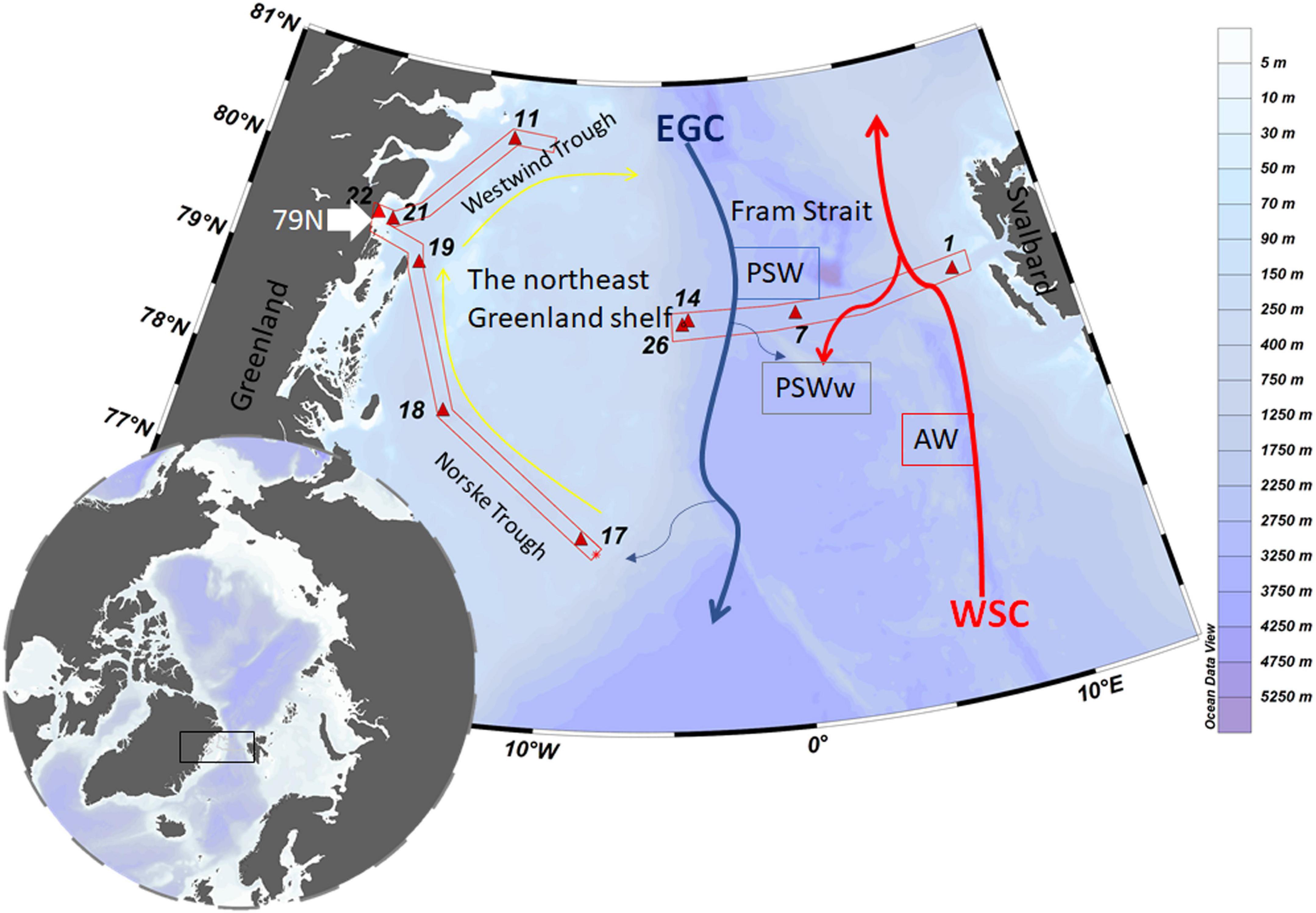
Figure 1. Map of the study area and schematic currents in Fram Strait. The black square indicates the sampling location, and stations are indicated by red triangles. The West-Spitsbergen Current (WSC, red arrows) brings warm Atlantic Water (AW) into the Arctic Ocean. The southward flowing East Greenland (EGC, gray arrows) carries part of the recirculated WSC as well as outflow waters from the Arctic Ocean. The anti-cyclonic circulation through the Norske – Westwind Trough system is indicated by yellow arrows. These schematic currents are simplified from Schaffer et al. (2017) and based on Bourke et al. (1987). Figure was made using the software Ocean Data View (Schlitzer, 2018).

DFe and Fe-Binding Ligand Analysis

Seawater samples for Fe speciation analysis were immediately stored at −20°C without acidification, since pH affects the partitioning of Fe among its different species. In un-acidified samples, however, bottle wall adsorption can cause Fe loss (Fischer et al., 2007; Jensen et al., 2020). The analysis of DFe was undertaken using two different subsamples, one immediately acidified onboard (Kirsch et al., unpublished) and a subsample taken from the ligand samples Ardiningsih et al. (2020) and available at doi: 10.25850/nioz/7b.b.u). DFe was determined in acidified samples, by isotope dilution high-resolution inductively coupled plasma-mass spectrometry (HR-ICP-MS, Thermo Fisher Element XR) after pre-concentration (Rapp et al., 2017), the detailed procedure is described elsewhere (Krisch et al., 2020). Subsamples for a second DFe determination from the ligand bottles, was analyzed using HR-ICP-MS (Thermo Fisher Element XR) after pre-concentration using an automated SeaFAST system (SC-4 DX SeaFAST pico; ESI), and the quantification was done via standard additions. The procedure is described in detail in Ardiningsih et al. (2020). DFe obtained from ligand samples was approximately 15% lower than DFe obtained from immediately acidified samples, as also found by others (Gerringa et al., 2016; Gerringa et al., 2019). DFe from ligand samples was used for the calculation of [L_t] and log K′_Fe’L. The results of the determination in samples immediately acidified onboard and in subsamples taken from the ligand is attributed to either adsorption of Fe on the ligand bottle wall and possibly, even though we worked in laminar flow benches, contamination subsample from the ligand bottle, since this bottle was handled several times for the different applications.

In order to extrapolate DFe speciation to ambient DFe concentrations, DFe from the immediately acidified samples, [L_t] and log K′_Fe’L were used to calculate the excess ligand concentrations [L′] (i.e., concentration of ligands not bound to Fe). The [L′] was subsequently used to calculate the side reaction coefficient of the ligands (α_Fe’L), which is the product of log K′_Fe’L and [L′]. The side reactions coefficient describes the effective affinity of a ligand for Fe, and takes into account the concentrations of the metal, the ligand and other competing cations thus describing the effective affinity between the natural ligands and Fe. The three different ALs used in the voltammetric methods (TAC, SA and NN) in this study will be indicated in subscript letters after the ligand parameters, e.g. [L_t]_TAC or log K′_Fe’L(TAC).

TAC Method

The analytical procedure of the here used TAC method is based on Croot and Johansson (2000), with modifications after Slagter et al. (2017). The method is described in detail by Ardiningsih et al. (2020) and uses a Hg drop electrode stand (VA663 Metrohm, Switzerland) connected to a μAutolab voltammeter and Nova 1.9 (Metrohm Autolab B.V., Netherlands) as the software user-interface. The titrations were done at pH 8.05 using 5 mM ammonium-borate buffer in the presence of 10 μM TAC and left to equilibrate for at least 8 h or overnight before voltammetric analysis. For each sample, duplicate scans were undertaken at a deposition time of 140 s, starting with the lowest added Fe(III) aliquot and working towards the highest added Fe(III) concentration. The Fe additions were 0; 0.2; 0.4; 0.6; 0.8; 1.0; 1.2; 1.5; 2.0; 2.5; 3.0; 4.0; 6.0; 8.0 nM, where the no Fe addition and the highest Fe addition vials were prepared in duplicate and both were analyzed. The limit of detection (LOD) was 0.016 nM eq. Fe, obtained as three times the noise in the scan.

SA Method

The SA method follows the protocol by Abualhaija and van den Berg (2014) with a low SA concentration (5 μM) and overnight (8 hours) equilibration, but using the BioAnalytical System (BASi) controlled growth mercury electrode coupled with an Epsilon ε2 (BASi) electrochemical analyzer (Buck et al., 2015). The voltammetry system was controlled by a computer using BASi Epsilon-EC as the interface software, and ECDsoft was used to quantify the peak height of the voltammetric scan.

Teflon vials (Fluorinated Ethylene Propylene (FEP), Savillex) were conditioned at least three times with seawater amended with buffer, DFe addition and SA. The first conditioning solution was changed immediately after rigorous shaking, followed by the next addition of conditioning solution, whereas the last conditioning solution was left at least for 8 h. The samples were buffered to a final pH of 8.2 with 5 mM of a boric acid-ammonium buffer. The titration consisted of 14 sub-sampled aliquots with Fe(III) standard additions of 0 to 3.0 nM with 0.5 nM intervals followed by concentrations of 4.0, 5.0, 6.0, 8.0, and 10 nM. The no addition and the highest addition were prepared in duplicate and both were analyzed. The chemical blank is measured in between samples to avoid carry over. For each sample, duplicate scans were done in a Teflon vial as voltammetric cell with a deposition time of 90 s. The LOD was 0.12 nM eq. Fe, obtained as three times the noise of our lowest standard (0.5 nM) in the scan.

NN Method

The analytical procedure for the NN method followed (Boye et al., 2001) and was adapted from the original NN method (Yokoi and van den Berg, 1992; Gledhill and van den Berg, 1994). Voltammetric analysis was performed using a mercury drop electrode stand model VA663 (Metrohm, Switzerland) connected to a μAutolab voltammeter (Metrohm Autolab B.V., the Netherlands).

Sample aliquots of 10 mL were buffered to pH 8.0 with 4-(2-Hydroxyethyl)piperazine-1-ethanesulfonic acid (HEPES; final concentration 0.01 M) and a final concentration of 2 μM NN was added. The addition of Fe (III) standards ranged from 0 to 10 nM with increments of 0.5 nM from 0 to 4.5 nM, followed by concentrations of 6.0; 8.0 and 10 nM. The sample mixtures were left to equilibrate overnight (≥ 12 h). The voltammetric scans were done in duplicate for each sample with a deposition time of 240 s. The LOD for the detection of FeNN₃, calculated using three times standard deviation of our lowest standard (0.5 nM)/slope is 0.13 nM eq. Fe for samples analyzed using the conditions used in this study.

Calculation of Speciation Parameters

We define the side reaction coefficient describing the effective affinity of Fe binding to AL as D, in order to prevent confusion with the side reaction coefficient of the natural ligands. It is the product of log K′_Fe’(AL)x and [AL], and calculated as (Table 1).

TABLE 1

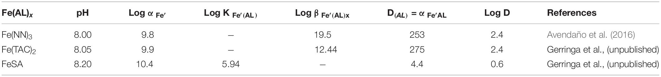
Table 1. Summary of the formed Fe(AL)_x complexes and the detection window of each voltammetric methods.

$$D=[AL]x{K}_{{\mathit{Fe}}^{\prime }(\mathit{AL})x}^{\prime }\mathit{or}D=[\mathit{AL}]{}^{x}x{\beta }_{{\mathit{Fe}}^{\prime }(\mathit{AL})x}^{\prime }(1)$$

The ‘upper’ limit of the detection window (Dw) is defined by the precision and detection limit of the analytical method (Laglera and Filella, 2015), whilst in an internally calibrated system, the lower limit is set by the assumption that all the weak ligand sites have been titrated within the range of added Fe concentrations, which can in practice be restricted by the linear range of the technique (Hudson et al., 2003). For this study, we assumed that the width of the Dw is one order of magnitude above and below the center of detection window, D, as conventionally assumed in the literature (Apte et al., 1988; van den Berg et al., 1990; Hudson et al., 2003; Pizeta et al., 2015).

The inorganic Fe side reaction coefficient (α${}_{{\mathrm{Fe}}^{\prime }})$ is used to transform the conditional stability constant of AL with respect to Fe³⁺ into the one with respect to Fé (log K′ _Fe’L). As the buffer pH differed between the methods, the pH of analysis was slightly different for each AL, thus the value of α_Fe’ is different for each pH (Table 1). Ardiningsih et al. (2020) used the value of α_Fe’ derived from Visual MINTEQ software (Gustafsson, 2011) with the ionic strength (I) is being calculated along with the determination of α_Fe’. In this study, the values of α_Fe’ were calculated based on the solubility products of the Fe-hydroxides at the fixed pH of analysis and I = 0.7 (Liu and Millero, 1999). As a result of different α_Fe’ values compared to previous results obtained with the TAC method, the resulted value of log K′_Fe’L and log α_Fe’L in this study are 0.1 higher than the results of TAC method reported by Ardiningsih et al. (2020).

A non-linear model of the Langmuir isotherm (Gerringa et al., 2014) was used to interpret the ligand parameters, as described for the data obtained with the TAC method by Ardiningsih et al. (2020). A one- and two-ligand model was applied to the data, and the ligand parameters calculated were [L_t], log K′_Fe’L and log α_Fe’L. In case of two ligand groups, the relatively strong ligand group was denoted with 1, the relative weak group with 2, as follows: [L₁]_TAC, and [L₂]_TAC, or log K′_1(TAC) and log K′_2(TAC). The sum of the concentration of [L₁] and [L₂] from the two-ligand model will be denoted as. The absolute difference between [L_t] values derived with two different method is referred to as δ[L_t] (i.e. δ[L_t]_SA–TAC is the absolute difference between [L_t]_SA and [L_t]_TAC). Two ligand groups could not be resolved for the NN method. The mean sensitivity (S) obtained for the samples with the different methods were S = 3.97 ± 0.70 (N = 70) for the TAC method, S = 76.4 ± 23.0 (N = 69) for the SA method, and for the NN method S = 0.93 ± 0.17 (N = 15).

Results

Hydrography

The water mass distribution and circulation are described elsewhere in detail (Rudels et al., 2005; Beszczynska-Möller et al., 2012; Rudels et al., 2015; Laukert et al., 2017; Richter et al., 2018). The selected stations in this study represent the main hydrographic features present in Fram Strait and on the northeast Greenland continental shelf (Figure 1; more details in Ardiningsih et al., 2020). Warm and saline (Temperature > 2°C and Salinity > 35; Rudels et al., 2005; Laukert et al., 2017). Atlantic Water (AW) is present at depths shallower than ∼500 m in our stations. Cold and less saline (Temperature ≤ 0°C and Salinity < 34.5; Rudels et al., 2005) PSW is present on the western side (stations 14, 26) in the upper ∼300 m. AW recirculates in the upper 200 m in the central Fram Strait, forming warmer Polar Surface Water (PSWw) (Swift and Aagaard, 1981). At about 500 to 900 m depth on both sides of Fram Strait, Atlantic Intermediate Water (AIW) (Rudels et al., 2005) exists above the Norwegian Sea Deep Water (NSDW) (Swift and Aagaard, 1981). In this study, AIW and NSWD are referred to as deep waters.

The Norske-Westwind Trough system is situated on the Northeast Greenland shelf (Figure 1). The surface water, PSW, follows this circulation flowing along the Norske Trough to the bay of the 79N Glacier and thereafter continues into the Westwind Trough. Deeper than 200 m, modified-AIW (mAIW) enters the Norske-Westwind Trough system, modified by physical mixing before being propagated toward the inner shelf (Topp and Johnson, 1997; Schaffer et al., 2017). The shallow sill in the Norske Trough restricts the flow of mAIW, causing the mAIW in the Norske Trough was 1^oC warmer than mAIW in the Westwind Trough (Schaffer et al., 2017), therefore in this study, it is referred to as warm-mAIW and cold-mAIW, respectively.

Fe Speciation Using a One-Ligand Model

Total ligand concentration, [L_t], is calculated for each method and grouped based on the water masses existing in the different biogeochemical provinces (Figure 2). We observed similar trends for [L_t]_TAC, [L_t]_SA and [L_t]_NN in various waters (Figures 2A–C; the number of samples for each water masses is given in Table 2), with an increase in the median [L_t] from Fram Strait to the Norske Trough and highest values at the glacier front and in Westwind Trough. The absolute values of [L_t] derived via the three different methods differed considerably. The [L_t]_SA (median = 2.82 nM eq. Fe) was highest followed by [L_t]_TAC (median = 1.79 nM eq. Fe) and [L_t]_NN (median = 0.96 nM eq. Fe). In Fram Strait, the ratio of [L_t]_TAC /[L_t]_SA varied between 0.6 to 1, however, on the shelf, this ratio was nearly constant at approximately 0.6 (median, Figure 3A). The ratio of [L_t]_NN /[L_t]_SA was 0.2 – 0.5 in Fram Strait and 0.2 – 0.8 over the shelf (Figure 3B).

FIGURE 2

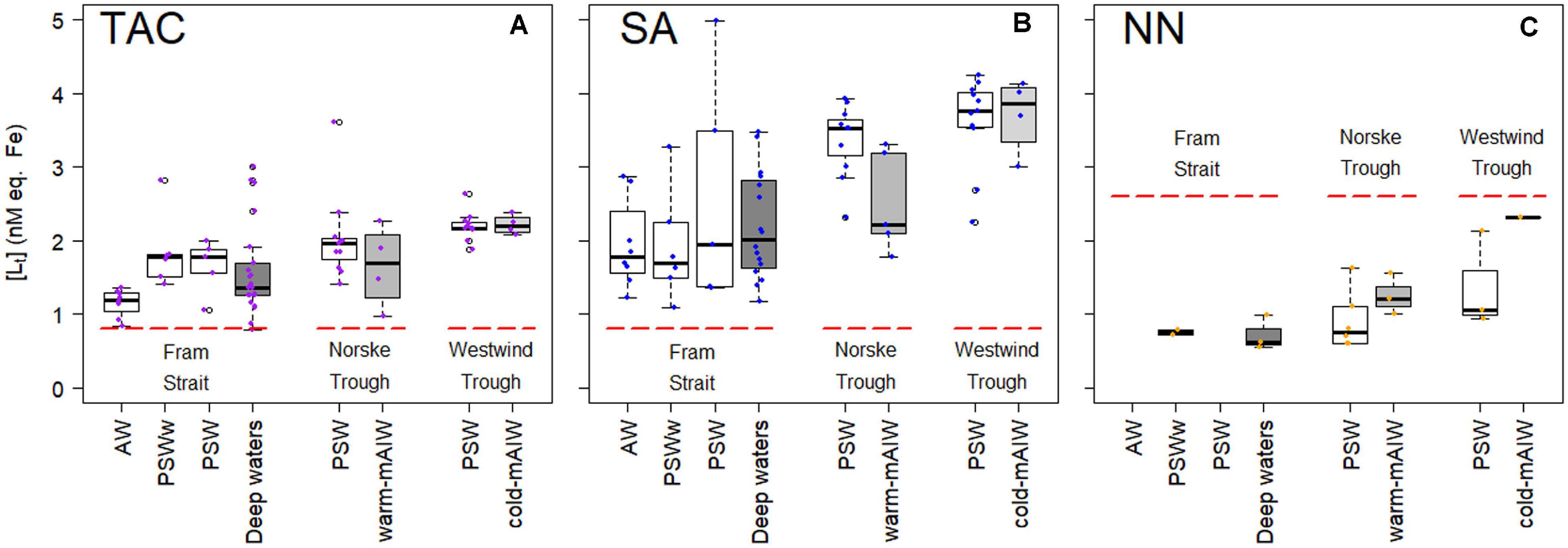
Figure 2. Box plot of ligand concentrations, [L_t], in nM eq. Fe from three different applications of added ligands (A) TAC, (B) SA, and (C) NN, as fitted (non-linear) by a one-ligand model using the Langmuir isotherm. The data is grouped by the biogeochemical provinces as described by Ardiningsih et al. (2020). A thick horizontal line indicates the median, the box contains the first to third quartiles, the whiskers are the range of data excluding the outliers and the circles indicate the outliers being 1.5* interquartile range from the box (Teetor, 2011). Figures were made using the software package R.

TABLE 2

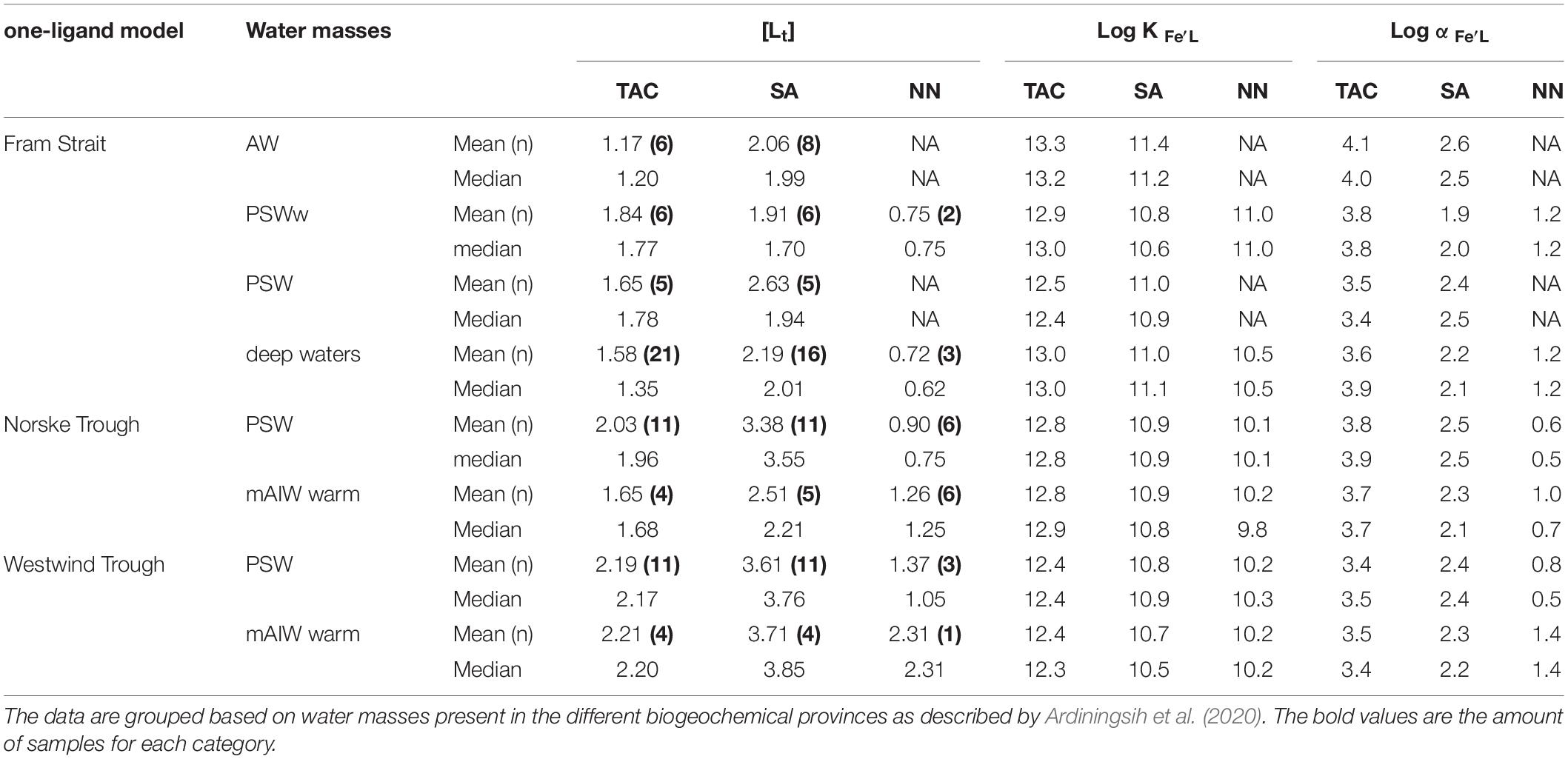
Table 2. Summary of the mean and median total ligand concentrations [L_t], conditional stability constants log K′_Fe’L, and the side reaction coefficients log, from the three applications of added ligands (TAC, SA and NN) according to the one-ligand model.

FIGURE 3

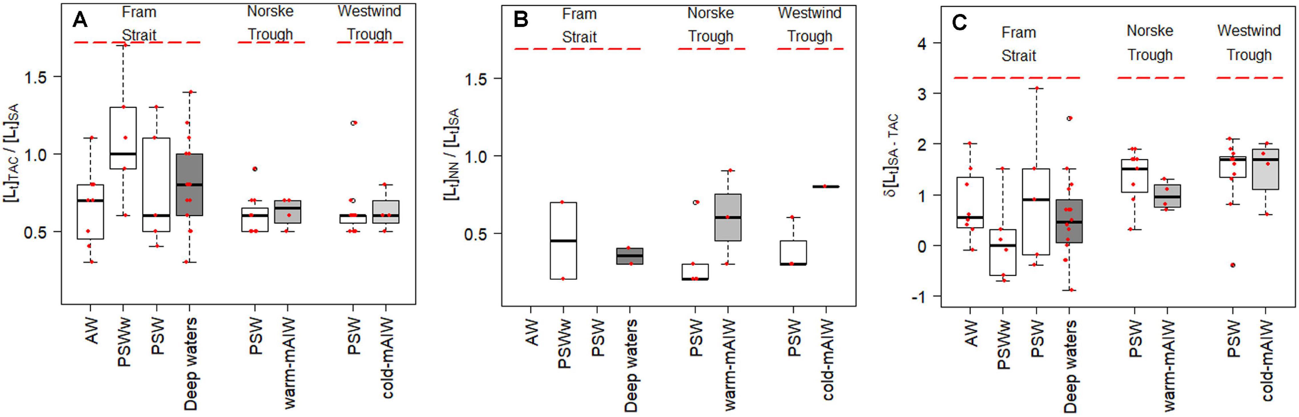
Figure 3. Boxplot showing the difference in ligand concentrations obtained by TAC, SA and NN, [L_t]_TAC, [L_t]_SA and [L_t]_NN, respectively. (A) the absolute difference in concentrations [L_t]_TAC - [L_t]_SA (nM eq. Fe), the relative ratio of (B) [L_t]_TAC / [L_t]_SA and (C) [L_t] _NN / [L_t]_SA. The details of the boxplot are described in Figure 2 caption.

For individual voltammetric methods, the variation in log K′_Fe’L values reached up to two orders of magnitude between samples (Figures 4A–C). The variation in log K′_Fe’L values in Fram Strait was larger than on the shelf. The most constant but lowest log values were observed in Westwind Trough. The value of log K′_Fe’L was highest for TAC, log K′_Fe’L(TAC) (median = 12.8), followed by log K′_Fe’L(SA) (median = 10.9) and log K′_Fe’L(NN) (median = 10.1; Supplementary Figure 1a). The differences in log K′_Fe’L values between the methods are significant (p < 0.05; Supplementary Figure 1a). For NN, median log K′_Fe’L(NN) values were significantly lower and ranged from 9.8 to 11.0 (Figure 4C and Table 2). For the determination of log K′_Fe’L, the curved part is essential. In the non-linear transformation of the Langmuir isotherm, log K′_Fe’L is derived by dividing the tangent of the curve at the lowest determined Fe concentration by the total ligand concentration. However, because ligand concentrations are typically ca. 1 nM eq. Fe in excess of the dissolved Fe concentration, an inability to detect the first titration point and a lower number of points in the curved part of the titration will mean that the tangent of the curve at the first detectable Fe concentration will be considerably lower than the tangent that would have been observed at the ambient DFe concentration and this will lead to an underestimation in log K′_Fe’L (e.g., for a samples with 0.5 nM DFe and a ligand concentration of 1.5 nM eq. Fe, 66 % of the ligands are titrated already at the first titration point of DFe+0.5 nM added). Thus, this difference likely arises because the peak with 0 Fe addition was usually not detected, which compromises the estimate of log K′_Fe’L(NN). Furthermore, for some samples the titration curves were nearly linear and the difference between the determined FeNN₃ concentration and the expected Fe concentration was too low to detect so that values of log K′_Fe’L(NN) and log α_Fe’L(NN) could not be estimated.

FIGURE 4

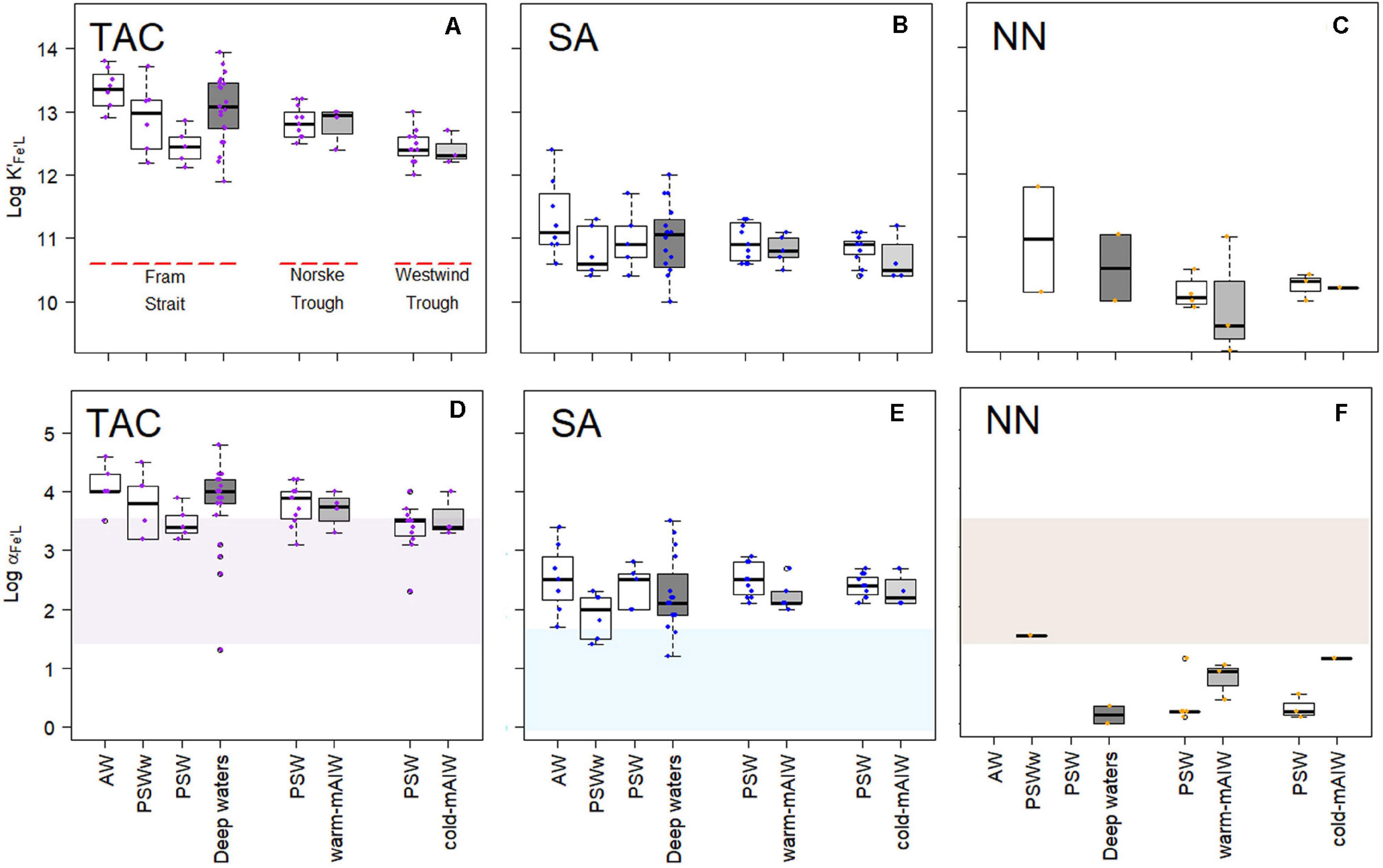
Figure 4. Boxplot of the conditional stability constants (log K′_Fe’L, A–C) and side reaction coefficients (log α _{Fe’L, d,e,f}) from three different methods using TAC, SA and NN as the AL. The shades in (D–F) indicate the detection window (log Dw) for each method. The details of the boxplot are described in Figure 2.

A relatively wide range in log α _Fe’L for both TAC and SA methods was observed in Fram Strait, whereas on the shelf, log α_Fe’L decreased with depth. The median log α_Fe’L(TAC) (3.8) was highest compared to log α_Fe’L(SA) (2.3) and log α_Fe’L(NN) (0.6) (Supplementary Figure 1b). The values of log α_Fe’L(TAC) and log α_Fe’L(SA) fell within and on the upper limit of log Dw (Figures 4D,E), whereas the values of log α_Fe’L(NN) mostly fell below the lower limit of log Dw (Figure 4F).

Fe Speciation Using a Two-Ligand Model

For both the TAC and SA methods, two ligand groups could be resolved in some of the samples, mostly the shelf samples (Figures 5A,B). Only 10% (4 out of 39) of samples from the Fram Strait could be resolved for two ligands using the TAC and SA methods, therefore, it is not possible to make a statistical comparison of the results of TAC and SA in the Fram Strait using the two-ligand model. On the shelf two ligands could be resolved for about 26% (8 out of 30) of the samples using TAC and 77% (24 out of 31) of the samples using the SA method.

FIGURE 5

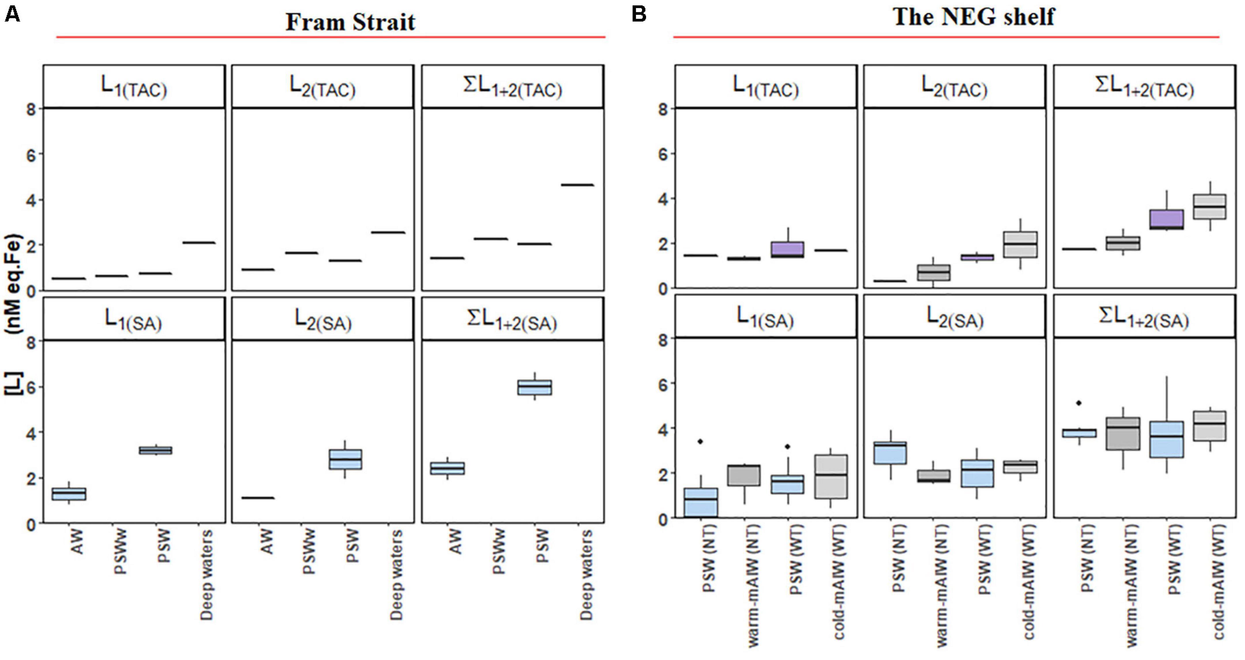
Figure 5. Boxplot of the results from a two-ligand model: ligand concentrations of the strong ligand group [L₁], and the relatively weak ligand group [L₂], together with the sum of [L₁] and [L₂] from samples (A) from Fram Strait and (B) from the northeast Greenland shelf. The details of the boxplot are described in Figure 2.

Using the TAC method, [L₁]_TAC, ranged from 0.48 to 2.66 nM eq. Fe (Figures 5A,B) with values of log K′_1(TAC) between 11.6 and 14 (Figures 6A,B). In comparison, [L₂]_TAC varied between 0.30 to 3.10 nM eq. Fe with log K′_2(TAC) between 11.1 and 11.7. The values of log α_2(TAC) and log α_1(TAC) were mostly within log Dw for TAC, with an exceptions some log α_1(TAC) values were higher than the upper limit of log Dw (Figures 6C,D).

FIGURE 6

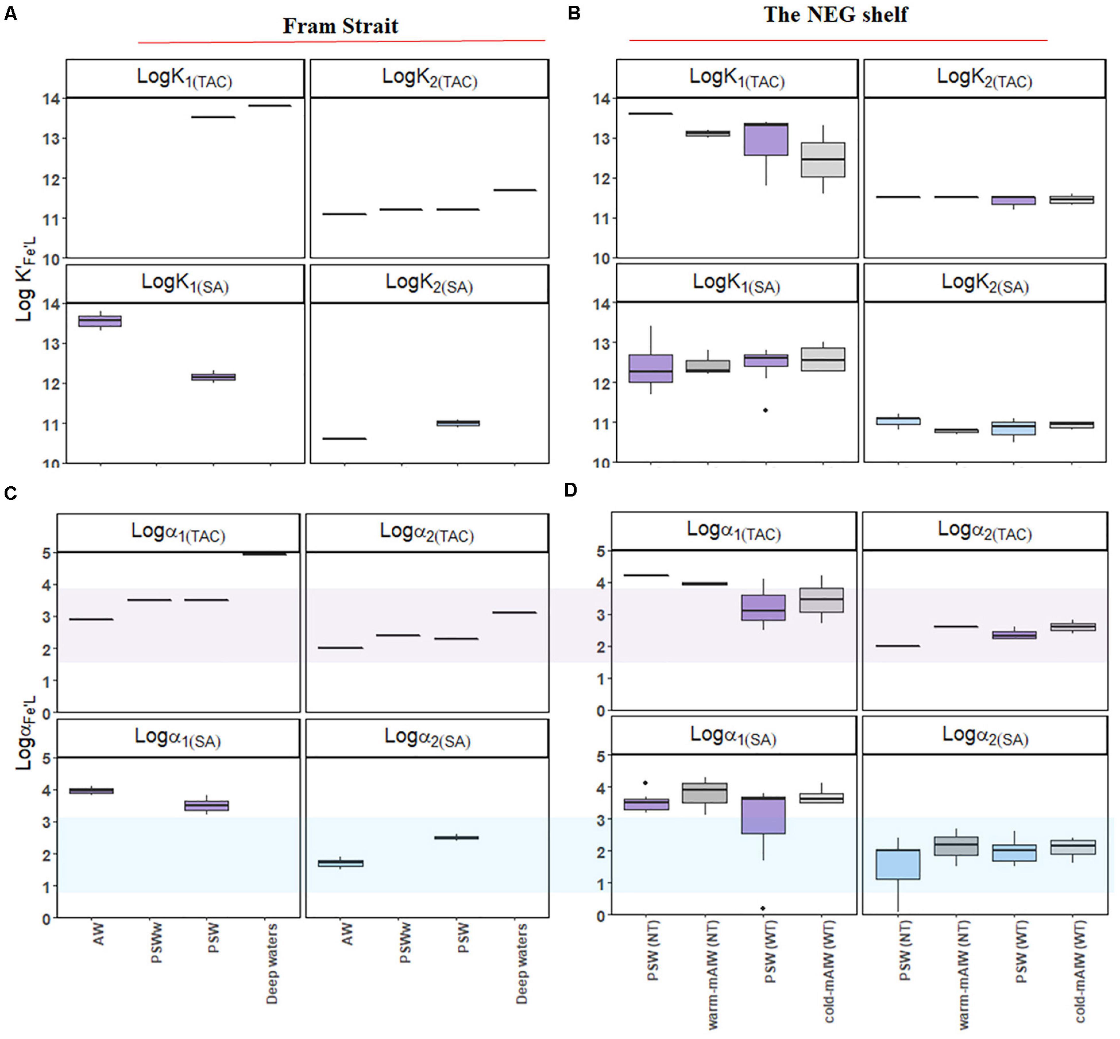
Figure 6. Boxplot of the results from a two-ligand model: the conditional stability constants of the relatively strong (log K′₁) and weak ligand groups (log K′₂) from samples (A) from Fram Strait and (B) from the northeast Greenland shelf; side reaction coefficients of the relatively strong (log α₁) and weak ligand groups (log α₂) from samples (C) from Fram Strait and (D) from the northeast Greenland shelf. The application of TAC and SA are indicated in subscribed letters. The shades in (C) and (D) indicate the detection window (log Dw) for each method. The details of the boxplot are described in Figure 2.

Using the SA method, [L₁]_SA ranged from 0.82 to 3.87 nM eq. Fe and [L₂]_SA from 0.08 to 3.43 nM eq. Fe. The values of log K′_1(SA) ranged from 11.3 to 13.8 and log K′_2(SA) from 10.5 to 11.2. Similar values of log α_{1 (SA)} were higher than log Dw, and log α_{2 (SA)} values fell within log Dw (Figure 5B).

Discussion

In the below discussion the ligand parameters (log K′_Fe’L, log α_Fe’L and [L_t]) derived from each method are related to Dw of the three ALs. Using different Dw, the ‘target ligand pool’ shifts, and it is thus appealing to use the different Dw to distinguish different fractions of binding sites. However, the precision of the Dw, its value and thus the conditional stability constant of AL (K′_Fe’AL or β_Fe’AL) with Fe must be considered. In order to properly evaluate K′_Fe’AL or β_Fe’AL, we must therefore consider uncertainties in the determination of K′_Fe’AL or β_Fe’AL. For example, ionic strength, the side reaction coefficients of the calibration ligand and the pH of the analysis could lead to subtle but important differences in Dw (Gledhill et al., 2015; Laglera and Filella, 2015; Ye et al., 2020).

The calibration of the competing AL is done by comparing the well-defined log α value of calibrating ligand, such as EDTA and diethylenetriaminepentaacetic acid (DTPA) with D. The corrections for ionic strength, the choice of the calibrating ligand side reactions and differences in pH have consequences for the resulting K′_Fe’AL and/or β_Fe’AL. Errors obtained during the derivation of D for the methods applied here range from < log 0.1 to log 0.9 (Gledhill and van den Berg, 1994; Rue and Bruland, 1995; Croot and Johansson, 2000; Abualhaija and van den Berg, 2014). From unpublished results of repeated calibrations, we have also found standard deviations in K′_Fe’AL and/or β_Fe’AL between log 0.5 and log 1 for D.

In addition, uncertainties can emanate during the interpretation of titration data. The competition between AL and the natural ligands determines log K′_Fe’L obtained where Fe additions filled the natural ligand sites, forming the curved part of the titration. The number of data points in the curved part hardly affects the calculation of [L_t], but a lack of data points here propagates high standard deviation in the estimation of log K′_Fe’L. This causes a high standard deviation in log K′_Fe’L in relatively saturated natural organic ligands. In the linear part of the titration, the number of data points affects both the values of [L_t] and log K′_Fe’L (Gerringa et al., 2014). Therefore, in our data we expect larger errors in K′_Fe’L estimated by SA and NN because these methods had fewer data points in the range of 0-1.5 nM added Fe (steps of 0.5 versus 0.2 nM Fe added). Indeed, larger error in estimation of log K′_Fe’L(SA) and log K′_Fe’L(NN) relative to log K′_Fe’L(TAC) were observed¹. Moreover, the sensitivity, which transforms the peak current (nA) into Fe concentration (nM), is obtained also from the slope of the linear part of the titration (Hudson et al., 2003). At high [L_t] it is possible that the linear part is not reached yet, and the titration curve is not truly linear, introducing an error in the estimation of S and [L_t]. The nonlinear Langmuir approach should compensate for this source of error in the data (Turoczy and Sherwood, 1997; Hudson et al., 2003; Gerringa et al., 2014).

The quality of the titration curves is given by the standard deviation of [L_t] and log K′_Fe’L. The variation of duplicate scans, especially in the first few points and at the high end of the titration could have large impact on the quality of the titration curves, adding uncertainties in the [L_t] and log K′_Fe’L, respectively. The zero Fe addition was done and measured twice to ensure that the measurement was not influenced by unconditioned cell. The variation of duplicate scans at low Fe addition could go up to 50%. The zero Fe addition was different from the blank only in a few samples containing near saturated ligands. The variation of duplicate scans at the high end of the titration affects the linear part of the titration curve, and thus the determination of [L_t], log K′_Fe’L and S. Therefore, the highest point Fe addition was done twice and measured with duplicate scans. At the highest Fe addition, the difference between duplicate scans was sometimes quite large, i.e. outliers were more than 20% different from the linear stretch (between 2 and 6 nM additions).

Other sources of uncertainty might come from the nature of the ligands. The heterogeneity of binding sites of large humic type molecules induces uncertainty depending on the saturation of the natural ligands with Fe. In this case, DFe concentration influences the outcome of the titration together with the detection window (Gledhill and Gerringa, 2017). Overall, the following discussion is limited to the above-mentioned uncertainties and the assumptions used on the calculations.

One-Ligand Model

The different detection windows reflect the ability of the methods to detect ligands (Gledhill and Gerringa, 2017) that are characterized by a range of log α_Fe’L. The detection windows of the SA, NN and TAC methods overlap (log Dw_(SA) = 0 – 1.6; log Dw_(NN) and log Dw_(TAC) = 1.4 – 3. 4). Nevertheless, the resulting median values for log α_Fe’L from the natural samples differ one order of magnitude between methods (SA: 1.2 – 3.5; TAC: 1.3 – 4.8; NN: 0.2 - 1.9; Table 2). Having the lowest Dw, the SA method detected ligands with log α_Fe’L values in between the other two methods (Figure 4E), and always had the highest [L_t] (Figure 2B), whereas log K′_Fe’L obtained from each method varied for SA: log K′_Fe’L 10 – 12.4, NN: log K′_Fe’L 9.2 – 11.8 and TAC: log K′_Fe’L 11.9 - 13.9¹. The three methods thus appear to detect different ligand pools in the same samples. However, considering an error of ± 0.5 - 1 due to uncertainties in calibration of the AL, NN and SA could have detected the same ligand group, albeit with different concentrations. With TAC we might have detected a different and stronger ligand group, compared to the results of the other two methods.

Many of the log α_Fe’L values were above the upper limit of Dw for data using the TAC and SA methods (Figures 4D,E), which agrees with reported data using the same analytical procedures (Buck et al., 2015; Gerringa et al., 2015). Buck et al. (2015) reported a range of log α_Fe’L from 2.5 to 3.5 (in their Figure 4C) with log D = 1.8, whereas Gerringa et al. (2015) reported log α_Fe’L values that varied from ∼ 3.0 to 4.0 (in their Figure 4) with log D = 2.4. Observations of log α_Fe’L above log Dw are relatively common (Caprara et al., 2016), which can be explained by the titration process. During a titration with Fe, [L′] decreases as the binding sites get filled with Fe, and consequently decreases the capacity of natural ligands to bind Fe (α_Fe’L = [L’]^∗K′_Fe’L), whereas the capacity of AL (α_Fe’AL) is assumed to be constant (Gledhill and Gerringa, 2017). The equivalence point of the titration is the point at which α_Fe’L = D. If during the titration, the α_Fe’L crosses Dw, then values of α_Fe’L can be estimated. However, if the curve is not evenly weighted (i.e., more titration points lie below D_w than above as is usually the case), then the estimate may be biased. Furthermore, if α_Fe’L is below Dw, then the data must be treated with care, since the values of log α_Fe’L became even lower with the Fe additions during the estimation. This is the case for almost all results obtained with NN and possibly arises as result of the lower sensitivity of the NN method, since this impacts both on the detection limit and the precision of the method. In practice this means that D_w for NN is likely to be narrower than that for SA and TAC and that NN could underestimate log K′_FeL(NN) using the CLE-AdCSV metal titration approach.

The median value of δ[L_t]_SA–TAC in PSW in western Fram Strait was 0.9 nM eq. Fe, whereas δ[L_t]_SA–TAC in PSW on the shelf increased to 1.5 nM eq. Fe and 1.7 nM eq. Fe, respectively, in the Norske Trough and in the Westwind Trough (Figure 3C). According to Laglera et al. (2011), the TAC method cannot detect part of the HS, and the NN method not sufficiently sensitive enough to elucidate stronger HS binding sites at nanomolar Fe concentrations in seawater. No consensus exists, however, on the underestimation of the HS ligands by the TAC method (Gerringa et al., 2007; Batchelli et al., 2010; Slagter et al., 2017; Dulaquais et al., 2018). Slagter et al. (2019) concluded that the TAC method can detect HS ligands when these ligands are either present at high concentrations or of a specific chemical composition. This could explain the lower [L_t] obtained with the TAC and NN methods compared to the SA method, and may even support the above reasoning using D. Since HS are heterogenous - with a distribution of ligand sites- HS does not therefore itself fit into ‘one group’ of ligands as determined by CLE-CSV. Moreover, the observable heterogeneity of ligand binding sites in samples is reduced at a higher detection window, thus a group of binding sites can be missed by an AL with a higher detection window (Gledhill and Gerringa, 2017). As such, the presence of HS as part of the ligand pool, can to some extent explain the difference in results between the methods. The PSW-flow via the TPD from the Arctic likely transfers HS ligands (Laglera et al., 2019a; Slagter et al., 2019). Approximately 62% of the Fe-binding ligands are humics in the TPD flow path in the Arctic (Sukekava et al., 2018), and thus [L_t]_TAC is probably underestimated for the NN method, the influence of HS on the results obtained were only for measurements at high NN concentrations when HS possibly cannot compete with NN (Laglera et al., 2011). However, NN ([NN] = 5 μM; log D = 2.9) has successfully been used to assess DFe speciation in Antarctic sea ice (Lannuzel et al., 2015; Genovese et al., 2018).

The [L_t]_TAC and [L_t]_SA capture the same trend of increasing concentrations from Fram Strait to Norske Trough and Westwind Trough (Figures 2A,B and Supplementary Figure 2a) with a fairly constant ratio of [L_t]_TAC over [L_t]_SA in PSW (median [L_t]_TAC/[L_t]_SA = 0.6; Figure 3B). The absolute differences, δ[L_t]_SA–TAC, varied in Fram Strait, where the HS influence possibly also varied, because the PSW-flow in western Fram Strait likely contains Arctic HS ligands. This suggests that HS play a role in the different results by the TAC and SA methods, however, the constant ratio ∼0.6 suggests a systematic offset between two methods, similar to the earlier studies (Buck et al., 2016; Slagter et al., 2019). Buck et al. (2016) concluded that TAC measurements from Gerringa et al. (2015) determined roughly half the ligand concentrations measured by the 25 μM SA method (Buck et al., 2012) at the BATS station in the Western Atlantic near Bermuda. Comparing the TAC and 25 μM SA methods, Slagter et al. (2019) found a ratio of 0.6 in the Arctic Ocean as well, remarkably both in and outside the influence of the HS-rich TPD. It must be noted that the 25 μM SA method is different in concentration and equilibration time from the SA method used in our study, indicating the offset likely appears irrespective to the used analytical procedure. In addition, even though a ratio near 0.6 is often found, the offset is irregular in Fram Strait outside PSW as we find ratios varying between 0.6 and 1 (Figure 3B). Thus, the question remains, does the TAC method underestimate the ligand concentration because it cannot detect part of the ligands or does SA method overestimate the ligand concentration?

An offset caused by HS should result in varying ratios of [L_t]_TAC/[L_t]_SA with a varying relative amount of HS, as shown in the value of δ[L_t]_SA–TAC. However, no relationship between HS and [L_t]_TAC/[L_t]_SA was observed in a previous study (Slagter et al., 2019) and we also did not see difference between the ratio of [L_t]_TAC/[L_t]_SA in HS-rich PSW compared to HS-poor AW (Figure 3B). Therefore, the difference between TAC and SA cannot solely be ascribed to their respective abilities to detect ligand groups in HS.

To conclude, the method with the highest detection window, i.e., TAC can detect a strong ligand group, and possibly misses weaker ligand groups, which were detected by the method with a lower detection window, SA. In contrast, despite having D_w similar to TAC, The use of NN results in both a lower [L] and log K′_Fe’L. The application of multiple methods as suggested by Buck et al. (2012) thus requires careful consideration. Nevertheless, our results showed that the one ligand model captured a similar trend in [L_t] for all three AL, and [L] increased from Fram Strait to the Norske Trough to the Westwind Trough (Figure 2).

Two-Ligand Model

A one and a two-ligand model were fitted in the same dataset. The one-ligand model gives an overall bulk result of what is present to facilitate the comparison of all samples. The two-ligand model worked only in a few samples where two ligand groups were different enough to be distinguished. Even though the two-ligand model did not work in some samples, this does not mean that the diversity is less, only that the diversity obscures that two groups can be detected.

A strong and progressively weaker ligand group was distinguished (Figures 6A,B) by the methods using TAC and SA as AL. Distinguishing two ligand groups is possible when ligands are distinct enough, although this depends on data quality and interpretation. The number of data points in a titration determines the quality of the interpretation whereas the different pH of the analyses and the different saturation with Fe of the ligand are complicating the interpretation (Gledhill and Gerringa, 2017; Ye et al., 2020). Assuming that two ligand groups exist, [L_t], log K′_Fe’L and log α_Fe’L in the one-ligand model represent a mixture of ligand groups (Figures 4A–C) probably with a continuum binding strength from strong to weak ligands (Buffle et al., 2007; Bundy et al., 2014). The range of log K′_Fe’L that has been reported spans up to five orders of magnitude from 9 to 14 and covers samples from the coastal to the open ocean (Gledhill and Buck (2012) and Hassler et al. (2017) in their Table 1). In this study the distinction of two ligand groups was possible in results from the TAC and SA methods. The conditional stability constants of the L₁ and L₂ ligand group obtained from each AL method are quite distinct and only for SA there is a slight overlap between the strong and weak log K′_Fe’L values (log K′_1(TAC) = 11.6 – 14 and log K′_2(TAC) = 11.1 – 11.7; log K′_1(SA) = 11.3 – 13.8 and log K′_2(SA) = 10.5 – 11.2; Figures 6A,B¹). The log K′_1(TAC) is overlapping with log K′_1(SA). In addition, the log K′_2(TAC) is in between log K′_1(SA) and log K′_2(SA), suggesting that the L₂ ligands detected by the TAC method are also detected by the SA method. Results from the NN method could not be resolved in two ligand groups in any of samples analyzed. To the best of our knowledge, the detection of two ligand groups from samples analyzed using NN as the AL, has never been reported (Boye et al., 2001; Lannuzel et al., 2015; Genovese et al., 2018).

There is a significant correlation between and [L_t] from the TAC and SA methods (p-value < 0.05; Supplementary Figures 2b,c). The SA method can resolve two ligands in more samples than the TAC method, especially for samples from the shelf. The SA method has a lower D, and therefore it should be better equipped to detect the weaker L₂ ligand group.

Given the many sources of uncertainties mentioned above, the error of the D is probably bigger than assumed, reducing likewise the precision of [L_t] and foremost log K′_Fe’L values. The composition of ligands as well as the heterogeneity of binding sites add an unknown error. The use of multiple methods did not simply resolve this issue. Our data shows that the ligand pool may contain two ligand groups or better stated two groups of binding sites.

Environmental Implications of Fe Speciation: Consequences for Fe Transport

Apart from possible method specific bias, similar trends in increasing [L_t]_TAC, [L_t]_NN and [L_t]_SA from Fram Strait to the Norske Trough and Westwind Trough may reflect a spatial and temporal differences in [L_t] in each biogeochemical province as described by Ardiningsih et al. (2020). It is reassuring that this trend is observed regardless of the used AL. The samples from Fram Strait have higher ratios of [L_t]_TAC/[L_t]_SA. This might be explained by a different composition of the ligand pool, compared to the shelf. However, as shown above, a distinction in the L₁-type and L₂-type ligands was not possible in Fram Strait. In deep waters of Fram Strait, [L_t]_TAC is almost equal to [L_t]_SA in near-seafloor samples (stations 7 and 14, Supplementary Figure 3), whereas at intermediate depth (∼400 – 600 m, stations 14 and 26, Supplementary Figure 3) [L_t]_TAC is even higher than [L_t]_SA. Biogeochemical and physical processes may alter the nature of Fe-binding ligands, changing the composition of the existing ligand groups, i.e. decomposition of sinking organic matter and vertical mixing in the water column (Tani et al., 2003). As speculated above, the alteration of ligand characteristics in the water column may explain the large variations of the ratios of [L_t]_TAC/[L_t]_SA in PSWw (Figure 3B). Overall, specific groups of ligands may not be detected by one method, whereas it is detected by the other, influencing the [L_t]_TAC/[L_t]_SA ratio.

Seawater on the shelf has a [L_t]_TAC/[L_t]_SA ratio of 0.5-0.6, and surface waters (> 100 m) in PSW in Fram Strait, show a similar ratio. These similarities may be indicative of a similar composition of the ligand pool in PSW. Bundy et al. (2014) suggested that water mass-specific in situ production of ligands is responsible for the increase in strong ligands in surface waters, whereas ligands from terrestrial origin mainly contributed to a weaker ligand group in surface waters. Ardiningsih et al. (2020) suggested that Fe-binding ligands in surface waters of the western Fram Strait mostly originated from surface microbial activity, with potential addition of HS ligands from the Arctic Ocean via the TPD-flow. In the shelf region, microbial processes seem to be the main source of ligands with possible addition of HS or exo-polymeric substances (EPS) produced in situ (Calace et al., 2001; Laglera and van den Berg, 2009; Poorvin et al., 2011; Burkhardt et al., 2014; Decho and Gutierrez, 2017; Laglera et al., 2019b). Moreover, EPS that are excreted by microbes, are expected to be present abundantly (Hassler et al., 2011; Decho and Gutierrez, 2017), especially in regions with sea ice-coverage (Krembs et al., 2002; Lin and Twining, 2012; Lannuzel et al., 2015; Genovese et al., 2018) such as surface waters over the northeast Greenland shelf. Thus, a mixture of ligand groups is expected in PSW, as confirmed by the distinction of two ligand groups in PSW of the western Fram Strait (by the SA method and only 4 samples by the TAC method) and over the shelf (by the SA and TAC methods) (Figure 5B).

The concentrations of excess ligand [L′] increased from Fram Strait to the Norske Trough and Westwind Trough (Supplementary Figure 4), indicating that ligands became less saturated. This increase is not only seen by TAC (Ardiningsih et al., 2020), but is here also confirmed by the SA method. The results of the two-ligand model have shown that the ligand pool contained the relatively weak ligand group, with a low complexation capacity despite its high concentration. Therefore, even though [L′] is available and provides binding sites for Fe, the low affinity of these ligands for Fe binding implies these ligands are relatively ineffective in preventing Fe scavenging and precipitation. Any additional Fe source to the seawater will effectively not result in more DFe, but rather in more Fe precipitation along with adsorption on sinking particles, thus capping DFe in seawater at the concentration range defined by the effective binding affinity (the product of [L′]^∗$K_{\text{FeL}}^{\prime }$) of the natural ligands. This was previously postulated by Ardiningsih et al. (2020) based solely on the TAC method to explain how ligand characteristics were crucial in controlling DFe export from the 79N Glacier terminus into Fram Strait. The use of the SA method provided a wider view in resolving the L₂ ligands, a relatively weak ligand group.

Conclusion

The assessment of TAC, SA and NN as AL with their specific detection windows in CLE-AdCSV titrations resulted in different ligand characteristics. The values of log K′_Fe’L and log α_Fe’L obtained from the SA method (log K′_Fe’L 10 – 12.4; log α_Fe’L 1.2 – 3.5) fell in between the other two methods (TAC: log K′_Fe’L 11.9 - 13.9, log α_Fe’L 1.3 – 4.8 and NN: log K′_Fe’L 9.2 – 11.8; log α_Fe’L 0.2 - 1.9). Hence, we cannot be sure that the ligands detected by the SA method are chemically similar to the ones detected by TAC and NN. The standard deviation of titration results, published by our group and others, generally considers only the fit of the data to the Langmuir isotherm, and not the underlying uncertainty of the precision of D of the ALs. Taking the uncertainty in D into account the interpretation is hampered by relatively large standard deviations generated by CLE-AdCSV titrations.

Our results showed that the SA and TAC methods detected ligands above or at the upper end of its Dw, whereas NN below its Dw. The results do not reflect the application of a broad detection window by the three ALs which are probably due to uncertainties propagated from the calibration of ALs, the titration procedures and the nature of ligands (i.e., composition of ligands and the heterogeneity of binding sites). The inability of TAC and NN to detect part of HS, is a probable explanation for the lower [L_t]_TAC and [L_t]_NN compared to [L_t]_SA in this study.

Our data from Fram Strait, where [L_t]_TAC/[L_t]_SA changes without relation to Arctic outflow of HS, provides an indication that other ligand groups than humics interfere with the detection efficiency of the AL. Other ligand groups also seem to be detected to a different extent by the TAC and SA methods. The constant ratios of [L_t]_TAC/[L_t]_SA ∼0.5 – 0.6 observed for the shelf region versus the variable ratios of [L_t]_TAC/[L_t]_SA in Fram Strait requires future research looking at the method specific bias in detecting specific types of Fe-binding ligands.

The similar trend of increasing [L_t] from Fram Strait to Norske Trough and Westwind Trough was captured by all three methods. This trend most likely reflects the spatial and temporal variability of Fe-binding ligands in the sampling region. The SA method is more suitable for the distinction of a relatively weak ligand group given that the detection window of SA is lower than TAC. The distinction of two ligand groups by both the TAC and SA methods provides information on the composition of Fe-binding ligands, particularly in PSW of western Fram Strait and in PSW over the shelf.

Data Availability Statement

The original contributions presented in the study are included in the article/Supplementary Material, further inquiries can be directed to the corresponding author/s.

Author Contributions

IA and KZ performed the analysis of the Fe-binding ligands. IA and LG prepared the content of the manuscript. LG designed the research and edited the manuscript. MG, RM, PL, EA, and G-JR performed the research and edited the manuscript.

Funding

This study was supported by Royal Netherland Institute for Sea Research. Collection and analysis of samples were further supported by GEOMAR Helmholtz Centre for Ocean Research (the Helmholtz Association and the German Research Foundation (DFG Award Number AC 217/1-1 to EA). IA was supported by a doctoral scholarship from Indonesia Endowment Fund for Education (LPDP), and KZ was supported by a scholarship from the China Scholarship Council.

Conflict of Interest

The authors declare that the research was conducted in the absence of any commercial or financial relationships that could be construed as a potential conflict of interest.

Acknowledgments

The authors would like to acknowledge Captain Schwarze and his crew of the RV Polarstern, as well as chief scientist Torsten Kanzow and all other participants, for their effort and support during sample collection. Patrick Laan and Stephan Krisch are acknowledged for analyzing DFe. We are grateful for the help of Mathijs van Manen and Hans Slagter during sample analysis.

Supplementary Material

The Supplementary Material for this article can be found online at: https://www.frontiersin.org/articles/10.3389/fmars.2020.609379/full#supplementary-material

Footnotes

1. ^ https://doi.org/10.25850/nioz/7b.b.7

References

Abualhaija, M. M., and van den Berg, C. M. G. (2014). Chemical speciation of iron in seawater using catalytic cathodic stripping voltammetry with ligand competition against salicylaldoxime. Mar. Chem. 164, 60–74. doi: 10.1016/j.marchem.2014.06.005

CrossRef Full Text | Google Scholar

Apte, S. C., Gardner, M. J., and Ravenscroft, J. E. (1988). An evaluation of voltammetric titration procedures for the determination of trace metal complexation in natural waters by use of computers simulation. Analyt. Chim. Acta 212, 1–21. doi: 10.1016/s0003-2670(00)84124-0

CrossRef Full Text | Google Scholar

Ardiningsih, I., Krisch, S., Lodeiro, P., Reichart, G.-J., Achterberg, E. P., Gledhill, M., et al. (2020). Natural Fe-binding organic ligands in Fram Strait and over the northeast Greenland shelf. Mar. Chem. 224:103815. doi: 10.1016/j.marchem.2020.103815

CrossRef Full Text | Google Scholar

Avendaño, L., Gledhill, M., Achterberg, E. P., Rérolle, V. M. C., and Schlosser, C. (2016). Influence of Ocean Acidification on the Organic Complexation of Iron and Copper in Northwest European Shelf Seas; a Combined Observational and Model Study. Front. Mar. Sci. 3. doi: 10.3389/fmars.2016.00058

CrossRef Full Text | Google Scholar

Batchelli, S., Muller, F. L. L., Chang, K.-C., and Lee, C.-L. (2010). Evidence for strong but dynamic iron-humic colloidal associations in humic-rich coastal waters. Environ. Sci. Technol. 44, 8485–8490. doi: 10.1021/es101081c

PubMed Abstract | CrossRef Full Text | Google Scholar

Beszczynska-Möller, A., Fahrbach, E., Schauer, U., and Hansen, E. (2012). Variability in Atlantic water temperature and transport at the entrance to the Arctic Ocean, 1997-2010. ICES J. Mar. Sci. 69, 852–863. doi: 10.1093/icesjms/fss056

CrossRef Full Text | Google Scholar

Boiteau, R. M., Mende, D. R., Hawco, N. J., McIlvin, M. R., Fitzsimmons, J. N., Saito, M. A., et al. (2016). Siderophore-based microbial adaptations to iron scarcity across the eastern Pacific Ocean. Proc. Natl. Acad. Sci. U.S.A. 113, 14237–14242. doi: 10.1073/pnas.1608594113

PubMed Abstract | CrossRef Full Text | Google Scholar

Bourke, R. H., Newton, J. L., Paquette, R. G., and Tunnicliffe, M. D. (1987). Circulation and water masses of the East Greenland shelf. J. Geophys. Res. Oceans 92, 6729–6740. doi: 10.1029/jc092ic07p06729

CrossRef Full Text | Google Scholar

Boyd, P. W., and Ellwood, M. J. (2010). The biogeochemical cycle of iron in the ocean. Nat. Geosci. 3, 675–682. doi: 10.1038/ngeo964

CrossRef Full Text | Google Scholar

Boye, M., van den Berg, C. M. G., de Jong, J. T. M., Leach, H., Croot, P., and de Baar, H. J. W. (2001). Organic complexation of iron in the Southern Ocean. Deep Sea Res. Part I Oceanogr. Res. Pap. 48, 1477–1497. doi: 10.1016/s0967-0637(00)00099-6

CrossRef Full Text | Google Scholar

Buck, K. N., Gerringa, L. J. A., and Rijkenberg, M. J. A. (2016). An intercomparison of dissolved iron speciation at the Bermuda Atlantic Time-series Study (BATS) site: results from GEOTRACES crossover station A. Front. Mar. Sci. 3:262. doi: 10.3389/fmars.2016.00262

CrossRef Full Text | Google Scholar

Buck, K. N., Lohan, M. C., Berger, C. J. M., and Bruland, K. W. (2007). Dissolved iron speciation in two distinct river plumes and an estuary: implications for riverine iron supply. Limnol. Oceanogr. 52, 843–855. doi: 10.4319/lo.2007.52.2.0843

CrossRef Full Text | Google Scholar

Buck, K. N., Moffett, J., Barbeau, K. A., Bundy, R. M., Kondo, Y., and Wu, J. (2012). The organic complexation of iron and copper: an intercomparison of competitive ligand exchange-adsorptive cathodic stripping voltammetry (CLE-ACSV) techniques. Limnol. Oceanogr. Methods 10, 496–515. doi: 10.4319/lom.2012.10.496

CrossRef Full Text | Google Scholar

Buck, K. N., Sedwick, P. N., Sohst, B., and Carlson, C. A. (2017). Organic complexation of iron in the eastern tropical South Pacific: results from US GEOTRACES Eastern Pacific Zonal Transect (GEOTRACES cruise GP16). Mar. Chem. 201, 229–241. doi: 10.1016/j.marchem.2017.11.007

CrossRef Full Text | Google Scholar

Buck, K. N., Sohst, B., and Sedwick, P. N. (2015). The organic complexation of dissolved iron along the U.S. GEOTRACES (GA03) North Atlantic Section. Deep Sea Res. Part II Top. Stud. Oceanogr. 116, 152–165. doi: 10.1016/j.dsr2.2014.11.016

CrossRef Full Text | Google Scholar

Buffle, J., Zhang, Z., and Startchev, K. (2007). Metal flux and dynamic speciation at (Bio)interfaces. Part I:? critical evaluation and compilation of physicochemical parameters for complexes with simple ligands and Fulvic/Humic Substances. Environ. Sci. Technol. 41, 7609–7620. doi: 10.1021/es070702p

PubMed Abstract | CrossRef Full Text | Google Scholar

Bundy, R. M., Biller, D. V., Buck, K. N., Bruland, K. W., and Barbeau, K. A. (2014). Distinct pools of dissolved iron-binding ligands in the surface and benthic boundary layer of the California current. Limnol. Oceanogr. 59, 769–787. doi: 10.4319/lo.2014.59.3.0769

CrossRef Full Text | Google Scholar

Bundy, R. M., Jiang, M., Carter, M., and Barbeau, K. A. (2016). Iron-binding ligands in the Southern California current system: mechanistic studies. Front. Mar. Sci. 3:27. doi: 10.3389/fmars.2016.00027

CrossRef Full Text | Google Scholar

Burkhardt, B. G., Watkins-Brandt, K. S., Defforey, D., Paytan, A., and White, A. E. (2014). Remineralization of phytoplankton-derived organic matter by natural populations of heterotrophic bacteria. Mar. Chem. 163, 1–9. doi: 10.1016/j.marchem.2014.03.007

CrossRef Full Text | Google Scholar

Calace, N., Castrovinci, D., Maresca, V., Petronio, B. M., Pietroletti, M., and Scardala, S. (2001). Aquatic humic substances in pack ice-seawater-sediment system. Intern. J. Environ. Analyt. Chem. 79, 315–329. doi: 10.1080/03067310108044392

CrossRef Full Text | Google Scholar

Caprara, S., Buck, K. N., Gerringa, L. J., Rijkenberg, M. J., and Monticelli, D. (2016). A compilation of iron speciation data for open oceanic waters. Front. Mar. Sci. 3:221. doi: 10.3389/fmars.2016.00221

CrossRef Full Text | Google Scholar

Croot, P. L., and Johansson, M. (2000). Determination of Iron speciation by cathodic stripping voltammetry in seawater using the competing Ligand 2-(2-Thiazolylazo)-p-cresol (TAC). Electroanalysis 12, 565–576. doi: 10.1002/(sici)1521-4109(200005)12:8<565::aid-elan565>3.0.co;2-l

CrossRef Full Text | Google Scholar

Cutter, G., Andersson, P., Codispoti, L., Croot, P., François, R., Lohan, M. C., et al. (2010). Sampling and Sample-Handling Protocols for GEOTRACES Cruises. Toulouse: GEOTRACES International Project Office.

Google Scholar

Decho, A. W., and Gutierrez, T. (2017). Microbial extracellular polymeric substances (EPSs) in ocean systems. Front. Microbiol. 8:922. doi: 10.3389/fmicb.2017.00922

PubMed Abstract | CrossRef Full Text | Google Scholar

Dulaquais, G., Waeles, M., Gerringa, L. J., Middag, R., Rijkenberg, M. J., and Riso, R. (2018). The biogeochemistry of electroactive humic substances and its connection to iron chemistry in the North East Atlantic and the Western Mediterranean Sea. J. Geophys. Res. Oceans 123, 5481–5499. doi: 10.1029/2018jc014211

CrossRef Full Text | Google Scholar

Filella, M., and Town, R. M. (2000). Determination of metal ion binding parameters for humic substances: part 1. Application of a simple calculation method for extraction of meaningful parameters from reverse pulse polarograms. J. Electroanalyt. Chem. 485, 21–33. doi: 10.1016/s0022-0728(00)00083-8

CrossRef Full Text | Google Scholar

Fischer, A. C., Kroon, J. J., Verburg, T. G., Teunissen, T., and Wolterbeek, H. T. (2007). On the relevance of iron adsorption to container materials in small-volume experiments on iron marine chemistry: 55Fe-aided assessment of capacity, affinity and kinetics. Mar. Chem. 107, 533–546. doi: 10.1016/j.marchem.2007.08.004

CrossRef Full Text | Google Scholar

Genovese, C., Grotti, M., Pittaluga, J., Ardini, F., Janssens, J., Wuttig, K., et al. (2018). Influence of organic complexation on dissolved iron distribution in East Antarctic pack ice. Mar. Chem. 203, 28–37. doi: 10.1016/j.marchem.2018.04.005

CrossRef Full Text | Google Scholar

Gerringa, L., Laan, P., Arrigo, K., van Dijken, G., and Alderkamp, A.-C. (2019). The organic complexation of iron in the Ross sea. Mar. Chem. 215:103672. doi: 10.1016/j.marchem.2019.103672

CrossRef Full Text | Google Scholar

Gerringa, L. J., Rijkenberg, M. J., Thuróczy, C.-E., and Maas, L. R. (2014). A critical look at the calculation of the binding characteristics and concentration of iron complexing ligands in seawater with suggested improvements. Environ. Chem. 11, 114–136. doi: 10.1071/en13072

CrossRef Full Text | Google Scholar

Gerringa, L. J. A., Rijkenberg, M. J. A., Bown, J., Margolin, A. R., Laan, P., and de Baar, H. J. W. (2016). Fe-Binding dissolved organic ligands in the oxic and suboxic waters of the Black Sea. Front. Mar. Sci. 3:84. doi: 10.3389/fmars.2016.00084

CrossRef Full Text | Google Scholar

Gerringa, L. J. A., Rijkenberg, M. J. A., Schoemann, V., Laan, P., and de Baar, H. J. W. (2015). Organic complexation of iron in the West Atlantic Ocean. Mar. Chem. 177, 434–446. doi: 10.1016/j.marchem.2015.04.007

CrossRef Full Text | Google Scholar

Gerringa, L. J. A., Rijkenberg, M. J. A., Wolterbeek, H. T., Verburg, T. G., Boye, M., and de Baar, H. J. W. (2007). Kinetic study reveals weak Fe-binding ligand, which affects the solubility of Fe in the Scheldt estuary. Mar. Chem. 103, 30–45. doi: 10.1016/j.marchem.2006.06.002

CrossRef Full Text | Google Scholar

Gledhill, M., Achterberg, E. P., Li, K., Mohamed, K. N., and Rijkenberg, M. J. A. (2015). Influence of ocean acidification on the complexation of iron and copper by organic ligands in estuarine waters. Mar. Chem. 177, 421–433. doi: 10.1016/j.marchem.2015.03.016

CrossRef Full Text | Google Scholar

Gledhill, M., and Buck, K. (2012). The organic complexation of iron in the marine environment: a review. Front. Microbiol. 3:69. doi: 10.3389/fmicb.2012.00069

PubMed Abstract | CrossRef Full Text | Google Scholar

Gledhill, M., and Gerringa, L. J. A. (2017). The effect of metal concentration on the parameters derived from complexometric titrations of trace elements in seawater—a model study. Front. Mar. Sci. 4:254. doi: 10.3389/fmicb.2012.00254

PubMed Abstract | CrossRef Full Text | Google Scholar

Gledhill, M., and van den Berg, C. M. G. (1994). Determination of complexation of iron(III) with natural organic complexing ligands in seawater using cathodic stripping voltammetry. Mar. Chem. 47, 41–54. doi: 10.1016/0304-4203(94)90012-4

CrossRef Full Text | Google Scholar

Gustafsson, J. P. (2011). Visual MINTEQ 3.0 User Guide. Stockholm: KTH, Department of Land and Water Recources.

Google Scholar

Hassler, C. S., Alasonati, E., Mancuso Nichols, C. A., and Slaveykova, V. I. (2011). Exopolysaccharides produced by bacteria isolated from the pelagic Southern Ocean — Role in Fe binding, chemical reactivity, and bioavailability. Mar. Chem. 123, 88–98. doi: 10.1016/j.marchem.2010.10.003

CrossRef Full Text | Google Scholar

Hassler, C. S., van den Berg, C. M. G., and Boyd, P. W. (2017). Toward a regional classification to provide a more inclusive examination of the ocean biogeochemistry of iron-binding ligands. Front. Mar. Sci. 4:19. doi: 10.3389/fmars.2017.00019

CrossRef Full Text | Google Scholar

Hudson, R. J. M., Rue, E. L., and Bruland, K. W. (2003). Modeling complexometric titrations of natural water samples. Environ. Sci. Technol. 37, 1553–1562. doi: 10.1021/es025751a

PubMed Abstract | CrossRef Full Text | Google Scholar

Hunter, K. A., and Boyd, P. W. (2007). Iron-binding ligands and their role in the ocean biogeochemistry of iron. Environ. Chem. 4, 221–232. doi: 10.1071/en07012

CrossRef Full Text | Google Scholar

Jensen, L. T., Wyatt, N. J., Landing, W. M., and Fitzsimmons, J. N. (2020). Assessment of the stability, sorption, and exchangeability of marine dissolved and colloidal metals. Mar. Chem. 220:103754. doi: 10.1016/j.marchem.2020.103754

CrossRef Full Text | Google Scholar

Kanzow, T. (2017). The expedition PS100 of the research vessel POLARSTERN to the Fram Strait in 2016. Rep. Polar Mar. Res. 705:175.

Google Scholar

Krembs, C., Eicken, H., Junge, K., and Deming, J. W. (2002). High concentrations of exopolymeric substances in Arctic winter sea ice: implications for the polar ocean carbon cycle and cryoprotection of diatoms. Deep Sea Res. Part I Oceanogr. Res. Pap. 49, 2163–2181. doi: 10.1016/s0967-0637(02)00122-x

CrossRef Full Text | Google Scholar

Krisch, S., Browning, T. J., Graeve, M., Ludwichowski, K.-U., Lodeiro, P., Hopwood, M. J., et al. (2020). The influence of Arctic Fe and Atlantic fixed N on summertime primary production in Fram Strait, North Greenland Sea. Sci. Rep. 10:15230.

Google Scholar

Laglera, L. M., Battaglia, G., and van den Berg, C. M. G. (2011). Effect of humic substances on the iron speciation in natural waters by CLE/CSV. Mar. Chem. 127, 134–143. doi: 10.1016/j.marchem.2011.09.003

CrossRef Full Text | Google Scholar

Laglera, L. M., and Filella, M. (2015). The relevance of ligand exchange kinetics in the measurement of iron speciation by CLE-AdCSV in seawater. Mar. Chem. 173, 100–113. doi: 10.1016/j.marchem.2014.09.005

CrossRef Full Text | Google Scholar

Laglera, L. M., Sukekava, C. F., Slagter, H. A., Downes, J., Aparicio-Gonzalez, A., and Gerringa, L. J. (2019a). First quantification of the controlling role of humic substances in the transport of iron across the surface of the arctic ocean. Environ. Sci. Technol. 53, 13136–13145. doi: 10.1021/acs.est.9b04240

PubMed Abstract | CrossRef Full Text | Google Scholar

Laglera, L. M., Tovar-Sanchez, A., Sukekava, C. F., Naik, H., Naqvi, S. W. A., and Wolf-Gladrow, D. A. (2019b). Iron organic speciation during the LOHAFEX experiment: iron ligands release under biomass control by copepod grazing. J. Mar. Syst. 207:103151. doi: 10.1016/j.jmarsys.2019.02.002

CrossRef Full Text | Google Scholar

Laglera, L. M., and van den Berg, C. M. G. (2009). Evidence for geochemical control of iron by humic substances in seawater. Limnol. Oceanogr. 54, 610–619. doi: 10.4319/lo.2009.54.2.0610

CrossRef Full Text | Google Scholar

Lannuzel, D., Grotti, M., Abelmoschi, M. L., and van der Merwe, P. (2015). Organic ligands control the concentrations of dissolved iron in Antarctic sea ice. Mar. Chem. 174, 120–130. doi: 10.1016/j.marchem.2015.05.005

CrossRef Full Text | Google Scholar

Laukert, G., Frank, M., Bauch, D., Hathorne, E. C., Rabe, B., von Appen, W.-J., et al. (2017). Ocean circulation and freshwater pathways in the Arctic mediterranean based on a combined Nd isotope, REE and oxygen isotope section across Fram Strait. Geochim. Cosmochim. Acta 202, 285–309. doi: 10.1016/j.gca.2016.12.028

CrossRef Full Text | Google Scholar

Lin, H., and Twining, B. S. (2012). Chemical speciation of iron in Antarctic waters surrounding free-drifting icebergs. Mar. Chem. 128–129, 81–91. doi: 10.1016/j.marchem.2011.10.005

CrossRef Full Text | Google Scholar

Liu, X., and Millero, F. J. (1999). The solubility of iron hydroxide in sodium chloride solutions. Geochim. Cosmochim. Acta 63, 3487–3497. doi: 10.1016/s0016-7037(99)00270-7

CrossRef Full Text | Google Scholar

Lodeiro, P., Rey-Castro, C., David, C., Achterberg, E. P., Puy, J., and Gledhill, M. (2020). Acid-base properties of dissolved organic matter extracted from the marine environment. Sci. Total Environ. 729:138437. doi: 10.1016/j.scitotenv.2020.138437

PubMed Abstract | CrossRef Full Text | Google Scholar

Mawji, E., Gledhill, M., Milton, J. A., Zubkov, M. V., Thompson, A., Wolff, G. A., et al. (2011). Production of siderophore type chelates in Atlantic ocean waters enriched with different carbon and nitrogen sources. Mar. Chem. 124, 90–99. doi: 10.1016/j.marchem.2010.12.005

CrossRef Full Text | Google Scholar

Middag, R., De Baar, H., Laan, P., and Bakker, K. (2009). Dissolved aluminium and the silicon cycle in the Arctic Ocean. Mar. Chem. 115, 176–195. doi: 10.1016/j.marchem.2009.08.002

CrossRef Full Text | Google Scholar

Nolting, R. F., Gerringa, L. J. A., Swagerman, M. J. W., Timmermans, K. R., and de Baar, H. J. W. (1998). Fe (III) speciation in the high nutrient, low chlorophyll Pacific region of the Southern Ocean. Mar. Chem. 62, 335–352. doi: 10.1016/s0304-4203(98)00046-2

CrossRef Full Text | Google Scholar

Omanović, D., Garnier, C., and Pižeta, I. (2015). ProMCC: an all-in-one tool for trace metal complexation studies. Mar. Chem. 173, 25–39. doi: 10.1016/j.marchem.2014.10.011

CrossRef Full Text | Google Scholar

Pizeta, I., Sander, S. G., Hudson, R. J. M., Omanovic, D., Baars, O., Barbeau, K. A., et al. (2015). Interpretation of complexometric titration data: an intercomparison of methods for estimating models of trace metal complexation by natural organic ligands. Mar. Chem. 173, 3–24. doi: 10.1016/j.marchem.2015.03.006

CrossRef Full Text | Google Scholar

Poorvin, L., Sander, S. G., Velasquez, I., Ibisanmi, E., LeCleir, G. R., and Wilhelm, S. W. (2011). A comparison of Fe bioavailability and binding of a catecholate siderophore with virus-mediated lysates from the marine bacterium Vibrio alginolyticus PWH3a. J. Exper. Mar. Bio. Ecol. 399, 43–47. doi: 10.1016/j.jembe.2011.01.016

CrossRef Full Text | Google Scholar

Rapp, I., Schlosser, C., Rusiecka, D., Gledhill, M., and Achterberg, E. P. (2017). Automated preconcentration of Fe, Zn, Cu, Ni, Cd, Pb, Co, and Mn in seawater with analysis using high-resolution sector field inductively-coupled plasma mass spectrometry. Anal. Chim. Acta 976, 1–13. doi: 10.1016/j.aca.2017.05.008

PubMed Abstract | CrossRef Full Text | Google Scholar

Richter, M. E., von Appen, W. J., and Wekerle, C. (2018). Does the east greenland current exist in the northern Fram Strait? Ocean Sci. 14, 1147–1165. doi: 10.5194/os-14-1147-2018

CrossRef Full Text | Google Scholar

Rudels, B., Björk, G., Nilsson, J., Winsor, P., Lake, I., and Nohr, C. (2005). The interaction between waters from the Arctic Ocean and the Nordic Seas north of Fram Strait and along the East Greenland current: results from the Arctic Ocean-02 Oden expedition. J. Mar. Syst. 55, 1–30. doi: 10.1016/j.jmarsys.2004.06.008

CrossRef Full Text | Google Scholar

Rudels, B., Korhonen, M., Schauer, U., Pisarev, S., Rabe, B., and Wisotzki, A. (2015). Circulation and transformation of Atlantic water in the Eurasian Basin and the contribution of the Fram Strait inflow branch to the Arctic ocean heat budget. Prog. Oceanogr. 132, 128–152. doi: 10.1016/j.pocean.2014.04.003

CrossRef Full Text | Google Scholar

Rue, E. L., and Bruland, K. W. (1995). Complexation of iron(III) by natural organic ligands in the Central North Pacific as determined by a new competitive ligand equilibration/adsorptive cathodic stripping voltammetric method. Mar. Chem. 50, 117–138. doi: 10.1016/0304-4203(95)00031-l

CrossRef Full Text | Google Scholar

Rue, E. L., and Bruland, K. W. (1997). The role of organic complexation on ambient iron chemistry in the equatorial Pacific ocean and the response of a mesoscale iron addition experiment. Limnol. Oceanogr. 42, 901–910. doi: 10.4319/lo.1997.42.5.0901

CrossRef Full Text | Google Scholar

Schaffer, J., von Appen, W.-J., Dodd, P. A., Hofstede, C., Mayer, C., de Steur, L., et al. (2017). Warm water pathways toward Nioghalvfjerdsfjorden Glacier, Northeast Greenland. J. Geophys. Res. Oceans 122, 4004–4020. doi: 10.1002/2016jc012462

CrossRef Full Text | Google Scholar

Schlitzer, R. (2018). Ocean Data View. Available online at: www.odv.awi.de

Google Scholar

Slagter, H. A., Laglera, L. M., Sukekava, C., and Gerringa, L. J. A. (2019). Fe-binding Organic ligands in the Humic-Rich TransPolar drift in the surface Arctic ocean using multiple voltammetric methods. J. Geophys. Res. Oceans 124, 1491–1508. doi: 10.1029/2018jc014576

CrossRef Full Text | Google Scholar

Slagter, H. A., Reader, H. E., Rijkenberg, M. J. A., Rutgers van der Loeff, M., de Baar, H. J. W., and Gerringa, L. J. A. (2017). Organic Fe speciation in the Eurasian Basins of the Arctic Ocean and its relation to terrestrial DOM. Mar. Chem. 197, 11–25. doi: 10.1016/j.marchem.2017.10.005

CrossRef Full Text | Google Scholar

Sukekava, C., Downes, J., Slagter, H. A., Gerringa, L. J. A., and Laglera, L. M. (2018). Determination of the contribution of humic substances to iron complexation in seawater by catalytic cathodic stripping voltammetry. Talanta 189, 359–364. doi: 10.1016/j.talanta.2018.07.021

PubMed Abstract | CrossRef Full Text | Google Scholar

Swift, J. H., and Aagaard, K. (1981). Seasonal transitions and water mass formation in the Iceland and Greenland seas. Deep Sea Res. Part A Oceanogr. Res. Pap. 28, 1107–1129. doi: 10.1016/0198-0149(81)90050-9

CrossRef Full Text | Google Scholar

Tani, H., Nishioka, J., Kuma, K., Takata, H., Yamashita, Y., Tanoue, E., et al. (2003). Iron(III) hydroxide solubility and humic-type fluorescent organic matter in the deep water column of the Okhotsk Sea and the northwestern North Pacific Ocean. Deep Sea Res. Part I Oceanogr. Res. Pap. 50, 1063–1078. doi: 10.1016/s0967-0637(03)00098-0

CrossRef Full Text | Google Scholar

Teetor, P. (2011). R Cookbook. O’Reilly Media, Inc.

Google Scholar

Topp, R., and Johnson, M. (1997). Winter intensification and water mass evolution from yearlong current meters in the Northeast Water Polynya. J. Mar. Syst. 10, 157–173. doi: 10.1016/s0924-7963(96)00083-8

CrossRef Full Text | Google Scholar

Turoczy, N. J., and Sherwood, J. E. (1997). Modification of the van den Berg/Ruzic method for the investigation of complexation parameters of natural waters. Analyt. Chim. Acta 354, 15–21. doi: 10.1016/s0003-2670(97)00455-8

CrossRef Full Text | Google Scholar

van den Berg, C. M. G. (1995). Evidence for organic complexation of iron in seawater. Mar. Chem. 50, 139–157. doi: 10.1016/0304-4203(95)00032-m

CrossRef Full Text | Google Scholar

van den Berg, C. M. G. (2006). Chemical speciation of iron in seawater by cathodic stripping voltammetry with dihydroxynaphthalene. Anal. Chem. 78, 156–163. doi: 10.1021/ac051441%2B

CrossRef Full Text | Google Scholar

van den Berg, C. M. G., Nimmo, M., Daly, P., and Turner, D. R. (1990). Effects of the detection window on the determination of organic copper speciation in estuarine waters. Analyt. Chim. Acta 232, 149–159. doi: 10.1016/s0003-2670(00)81231-3

CrossRef Full Text | Google Scholar

Whitby, H., Planquette, H., Cassar, N., Bucciarelli, E., Osburn, C. L., Janssen, D. J., et al. (2020). A call for refining the role of humic-like substances in the oceanic iron cycle. Sci. Rep. 10:6144.

Google Scholar

Ye, Y., Völker, C., and Gledhill, M. (2020). Exploring the iron-binding potential of the ocean using a combined pH and DOC parameterization. Glob. Biogeochem. Cycles 34:e2019GB006425.

Google Scholar

Yokoi, K., and van den Berg, C. M. G. (1992). The determination of iron in seawater using catalytic cathodic stripping voltammetry. Electroanalysis 4, 65–69. doi: 10.1002/elan.1140040113

CrossRef Full Text | Google Scholar