Hard to Manage? Dynamics of Soft-Shell Crab in the Newfoundland and Labrador Snow Crab Fishery

Introduction

Biology of Soft-Shell Crab

Newfoundland and Labrador (NL) snow crab (Chionoecetes opilio) molt over-winter or during spring, with spatiotemporal molting dynamics associated with movement and mating patterns (Mullowney et al., 2018a). Sexual size dimorphism enables a male-only harvest strategy, therefore molting dynamics of large males are of most interest to the fishery. The regulated minimum legal-size of 95-mm carapace width (CW) for males is much larger than maximum sizes typically reached by females (Mullowney et al., 2018a, 2019).

In male snow crab, sexual maturity occurs prior to morphometric maturity, with morphometric maturity delayed until the final terminal molt into adulthood. Terminal molt occurs over a broad size range of about 45–150 mm CW (Mullowney et al., 2019). Both adolescent (sexually mature but not adult) and adult males of legal-size are retained in the fishery. Adolescents below legal-size constitute pre-recruits while recently molted legal-size males constitute immediate recruits, although they are not ready to harvest right away. Upon molting, a larger pliable soft-shell (herein “SS”) replaces the pre-existing shell and internal meat is replaced by water. It takes several months for shells to harden and fill with meat following a molt (Mullowney et al., 2020).

There are two focal molting periods in male snow crab. First, in association with mating of first-time spawning (“primiparous”) mature females, adolescents molt over-winter in shallow water (Sainte-Marie and Hazel, 1992; Sainte-Marie et al., 1999; Mullowney et al., 2018a). Although intraspecific competition from large adult males frequently prohibits adolescent males from successfully mating (Comeau et al., 1998; Kolts et al., 2015), they often molt during the post-mating recovery period (Sainte-Marie and Hazel, 1992; Sainte-Marie et al., 1999). Terminal molt is common during this process because of the cold conditions in which it occurs (Sainte-Marie and Hazel, 1992; Mullowney et al., 2018a). In the second molting period, adolescent males molt in deep water during spring (Mullowney et al., 2018a). This molting process appears most focused on growth because the warm water in which it occurs reduces probability of terminal molt (Burmeister and Sainte-Marie, 2010; Dawe et al., 2012).

Collectively, the two molting processes result in a demographic profile of vertical size stratification, with large males normally distributed deepest (Dawe and Colbourne, 2002). The fishery typically targets large males in deep water, where encounters of large soft-shell males can be common (Mullowney et al., 2019).

The timing of molting is likely affected by temperature, but this relationship has received little directed study in wild populations. Tank-based studies have shown that snow crab maintained in warmer conditions molt earlier and have reduced post-molt recovery times relative to those molting in colder conditions (Dutil et al., 2010). Warmer conditions have also been shown to promote higher synchrony in the primiparous female mating/molting period for snow crab kept in tanks (Sainte-Marie et al., 2010). For context, the snow crab is highly stenothermic, most frequently found in temperatures ranging from −1 to 3°C (Mullowney et al., 2018a).

Management of Soft-Shell Crab

SS discard mortality constitutes biological and economic wastage (Mullowney et al., 2019). Therefore, avoidance of SS crab is a foremost management concern in the fishery (DFO., 2020). Despite this, no explicit knowledge on mortality rates associated with discarding SS snow crab in NL exists. Nonetheless, SS crab are commonly believed to be more susceptible to handling mortality than their hard-shell counterparts (Mullowney et al., 2019). Literature on snow crab discard mortality suggests climatic and physiological factors including air and water temperature, wind speed, sunlight, exposure time, and individual size and shell condition affect handling mortality in snow crab in general (Miller, 1977; Dufour et al., 1997; Grant, 2003; van Temelen, 2005; Urban, 2015).

The NL snow crab management system imposes a spring-summer seasonality for fishing (DFO., 2020), supported by historic observations of high SS incidence in summer and fall fisheries (Mullowney et al., 2012, 2019). The management system also enforces a SS Protocol to invoke spatial fishery closures. This protocol closes either 10 × 7 nautical mile (nm) (offshore) or 5 × 3.5 nm (inshore) grids to fishing once SS incidence reaches 15 or 20% of the catch (only based on large males), depending on area (DFO., 2020). At-sea observers measure the catch to determine if closure thresholds are met.

Two related factors knowingly associated with SS incidence in the fishery are exploitation and catch rates (Mullowney et al., 2018b, 2019). Elevated exploitation rates contribute to reduced fisheries catch per unit effort (CPUE). In turn, depletion of large hard-shell males by the fishery allows increased catchability of SS crab, reflecting relaxed intraspecific competition to access baited traps.

Beyond fisheries exploitation and catch rates, there appears to be underlying spatiotemporal processes regulating SS incidence in the fishery. This likely reflects variation in molting periods across time and space. In particular, there are chronic issues of high SS incidence in fisheries along northern portions of the NL marine shelf (Northwest Atlantic Fisheries Organization (NAFO) Divisions 2H, 2J, and 3K, Figure 1), where SS capture rates typically increase from spring to summer and periodically reach levels of 50% of the catch or more (Mullowney et al., 2012, 2019).

FIGURE 1

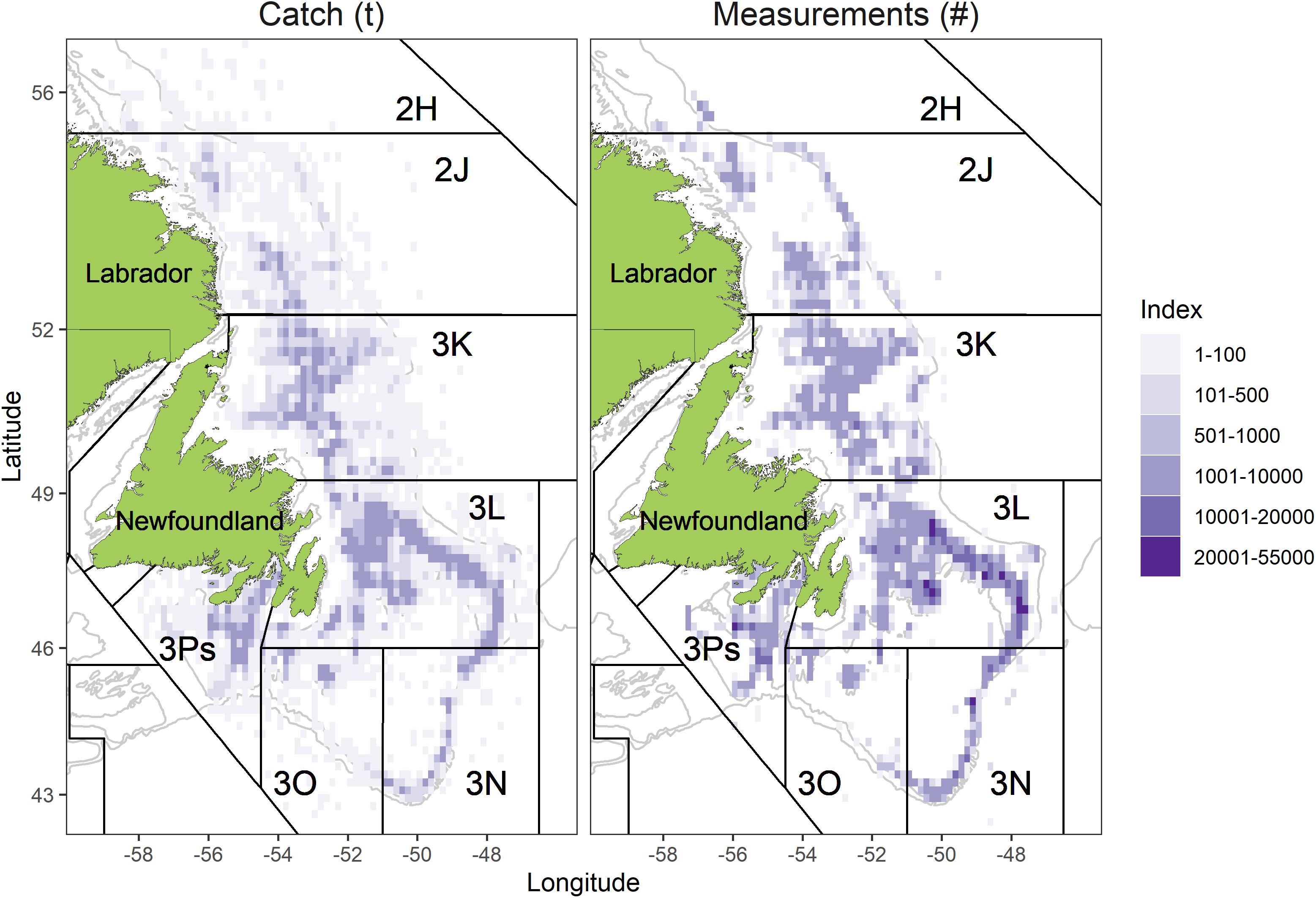
Figure 1. Distribution of total catch (left panel, data source is fishery logbooks) and measurements (right panel, data source is at-sea observer) from the snow crab fishery during 2000–2019.

The primary purpose of this study is to investigate dynamics of how seasonality and fisheries exploitation rates affect SS incidence in the NL snow crab fishery. The analysis is intended to better quantify and understand pathways of effects toward provision of improved management advice for governance of this lucrative fishery. The necessity of the work has become exacerbated by recently reduced levels of at-sea observer coverage in the fishery, affecting in-season monitoring capacities for resource management.

Materials and Methods

Study Area

The study was carried out on snow crab inhabiting the easternmost Canadian territorial waters of the NL marine shelf (Figure 1). This 182,000 nm² of dynamic continental shelf was broken into four Assessment Divisions (ADs) comprised of groupings of the NAFO Divisions, defined as ADs 2HJ, 3K, 3LNO, and 3Ps, and following stock assessment methods (Mullowney et al., 2019).

The two northernmost ADs (2HJ and 3K) are overall deeper and warmer than the two southern ADs (3LNO and 3Ps). This reflects less extensive coverage of the Cold Intermediate Layer (CIL), a body of < 0°C water that persists at intermediate depths (Mullowney et al., 2019; Cyr et al., 2020). Nearest to shore areas in all but AD 3Ps were omitted from analysis (Figure 1) due to lack of consistent coverage by trawl surveys, which form the basis of biomass estimation and fisheries exploitation rates.

Data Sources

Data on SS crab in the fishery came from at-sea observers. In 2000, observers began measuring snow crab using a three-stage shell classification index of soft, new-hard, or old-hard, subjectively approximating time since molting. The fishery occurs from April to August in most ADs. Therefore, SS crab are assumed to have molted in the current winter/spring and old-shell crab are assumed to have molted at least 1 year ago. Most uncertainty in approximating time since molting occurs in new-shell crab, which could have plausibly molted either in the present or preceding year. Along with classifying shell conditions, observers measure dorsal CW.

Observers are randomly deployed on vessels throughout the season, but only a small portion of trips are observed in any given year. In total, 2.6 million male measurements from the 20 years sampling period were used in analyses. Locations of the number of measurements were mapped to 10 × 10 nm cells and compared to the overall fishery distribution, and the annual percentage of observer coverage was calculated based on total weight of the measured catch versus fishery landings enumerated from an obligatory dockside monitoring offload program.

The percentage of SS crab was calculated as the total number of SS male crab divided by the total catch from each measured trap. Kept crab, or fishery CPUE (#/trap), was defined as male crab ≥ 95 mm CW in new- or old-shell condition on a per-trap basis while SS were overall percentage of males in soft-shell condition (regardless of size) in relation to the total catch of male crab in the trap. Only weeks with ≥ 50 measured crab in any given AD were examined. Weekly SS crab percentages were correlated against plausible explanatory variables of fishery CPUE, weekly and cumulative fishery exploitation rates, and calendar week toward isolating explanatory variables for a parsimonious predictive model.

Weekly and cumulative exploitation rates were based on the pace of fishery landings in relation to annual Exploitable Biomass Indices (EBIs) of crab available to the fishery. EBIs were taken from the most recent stock assessment and are based on depth-stratified random multi-species trawl surveys that occur in ADs 2HJ, 3K, and 3LNO during fall and AD 3Ps during spring. A spring survey does occur in AD 3LNO, but is less preferred for biomass estimation due to lower trawl catchability of snow crab by the survey trawl during spring. In a typical year about 600–800 tows occur over the 2HJ3KLNO area during fall, and about 400–600 over the 3LNOPs area during spring (see Mullowney et al., 2019 for further details on biomass estimation).

A 1 year lag is applied to fall biomass estimates to calculate Exploitation Rate Indices (ERIs), defined as landings/biomass, because surveys occur in the preceding calendar year. No recruitment into the biomass is expected to occur during the over-winter period, although natural mortality losses could occur between the time the biomass is measured and the fishery begins. For spring survey biomass estimates in AD 3Ps, the survey is partially in-season (late March to late April), thus some fishery removals occur prior to biomass estimation. Nonetheless, the effect is not major and no accounting for it was done in deriving ERIs. Prior to calculating ERIs, EBIs were smoothed to two-period moving averages to account for survey “year effects” (Mullowney et al., 2019).

The annual pace of fishery removals was determined from fishery logbooks detailing time and location of sets along with catch and effort information. Total landings were summed to weekly bins. Although the majority of logbooks are returned each year (total of 314,000 sets included), the logbook dataset is incomplete, such that the true level of fishery landings is under-estimated. To account for this, the annual ratio of logbook-summed landings to quota-monitored landings was calculated, with the resulting annual bump-up factors applied to weekly catch increments. This invoked an assumption that logbook under-estimation was uniform throughout the season. Weekly and cumulative ERIs were calculated based on the ratios of weekly landings to annual EBI estimates.

Predictive Modeling

Based on correlation analysis, explanatory variables of week and cumulative fishery ERI (“cERI”) were selected for modeling the response variable of percent SS in the catch. It should be highlighted that the time variable (calendar week) could merely be a proxy reflecting underlying variables such as ambient light or temperature conditions in the water column that may be specific mechanisms for any seasonal outcomes in soft-shell crab incidence in the fishery, but for which quantitative weekly data are not available. Moreover, the inclusion of calendar week in the model maintains focus on a directly controllable factor in management of the fishery.

To examine spatiotemporal patterns affecting collinearity among the two explanatory variables, AD- and year-specific curves of SS timing and prevalence levels were examined to investigate if contrast across and within ADs over the study period could help offset concerns of correlation between the two explanatory variables.

A hierarchical Generalized Additive Mixed Model (hGAMM) was run in the mgcv package (Wood, 2011, 2017) in R version 3.6 (R Core Team., 2019). A hGAMM was selected because it enabled the ability to model group-specific (AD) effect processes along with over-arching global effect processes, and the modeling approach partially offsets confounds of collinearity among explanatory variables (Pedersen et al., 2019). The model, defined in [1], regresses main and interaction effects of week and cERI against the response variable, first by AD then at the global level. A beta family data distribution was assumed due to the proportional nature of the response variable and a complementary log-log link was applied due to ad hoc observations of rapid increases in the response variable over small incremental changes in the two explanatory variables. All variables were binned to weekly units with observations of 0% SS in the catch included as 0.0001% to contain response data within the 0–1 range of the beta distribution.

$$[1]\%SS\sim \mathrm{week}{}_{\mathit{AD}}+\mathrm{cERI}{}_{\mathit{AD}}+(\mathrm{week}{}_{\mathit{AD}}{}^{*}\mathrm{cERI}{}_{\mathit{AD}})+\mathrm{week}{}_{\mathit{ge}}+\mathrm{cERI}{}_{\mathit{ge}}+(\mathrm{week}{}_{\mathit{ge}}{}^{*}\mathrm{cERI}{}_{\mathit{ge}})+\mathrm{r}(\mathrm{year},\mathrm{division})$$

Where,

%SS denotes the percentage of SS crab in the catch, week denotes calendar week, cERI denotes cumulative ERI, AD denotes Assessment Division, ge denotes global effect, and r denotes a random intercept effect. Thin-plate regression splines (s) were used to generate smooths for each main effect, while tensor product smooths (Wood, 2006) were used on interaction terms. A full interaction tensor product (“te”) was applied to the random year—division intercept term, while for week and cERI interactions the interaction tensor product (“ti”) did not consider the lower-order main effects. The AD-level effects were penalized on the first-order derivative (m = 1) while global effects were penalized on the second-order derivative (m = 2). Degrees of freedom complexity matrices were set at k = 10 for the AD-level effects and freely allowed to vary for global effects.

The model was assessed as a good fit based on adjusted r² and scaled deviance statistics, as well as distribution of annual AD-level residuals. Marginal effect smooths were examined to assess directional influences of the main effects, developed by re-fitting the model with other explanatory variables held constant while varying focal effects. These constants were time-series means of fishing week and maximum annual cERI within each AD.

Relevant Management Information

The history of weekly proportions of shell conditions in the catch were examined with loess regression curves, pooling all years of data. This was done to qualitatively investigate concerns that capture and potential discard of new-shell crab could constitute additional fishery and biological wastage above that quantified through soft-shell crab observation data. For example, a crab that molted in the winter or spring of the current year and assessed as a new-shell animal in the fishery would still render lower than optimal meat yield, with a recent study showing new-shell meat fullness to range between 50 and 70% from July to November (Mullowney et al., 2020), or could incur higher mortality than an old-shell crab if discarded.

The history of observed weekly catch proportions was also used to estimate surplus amounts of unaccounted for crab potentially killed in the fishery through soft-shell discard mortality. We did not have a reliable basis upon which to estimate true discard mortality rates on soft-shell crab, so we applied arbitrary discard mortality rates of 10, 50, and 90% to represent a range of low to high mortality rates. These arbitrary mortality rates were first applied against observed weekly proportions of soft-shell crab in the catch to determine overall annual totals in each AD, assuming all soft-shell crab were discarded and all new and old-shell legal-size crab were landed. The differential mortalities were subsequently scaled to annual totals of dockside-monitored fishery landings to estimate potential levels of unaccounted surplus mortality in the fishery. Surplus mortality estimates were presented both in terms of tonnage and exploitation rate percentages.

Finally, to investigate if localized temperature conditions could affect molt timing and subsequently optimal fishery timing in different ADs, the peak SS prevalence weeks predicted from hGAMM [1] were examined in relation to bottom temperature at-capture for pre-recruit and recruit crab. All years of data were pooled for this analysis. Crab and temperature data were taken from the seasonal trawl surveys, with bottom temperatures acquired during each tow. Accordingly, both the temperature and specimen data are annual “snap-shots” and not continuous throughout the year. Male crab that were ≥ 75 mm CW adolescents or SS or new-shell adults were selected. These crab represent those that could soon become, presently are, or recently were SS crab in the exploitable biomass. Mean bottom temperatures at-capture were calculated and compared with peak SS week in a log-log linear regression model, by survey series and season, with AD 3LNO having observations from both fall and spring surveys included.

Results

Data Sources

Observer sampling data are overall spatially representative of the fishery. The time-series spatial footprint of measurements reflected that of the fishery in all ADs (Figure 1). Virtually all grid cells located on primary fishing grounds received more than 1,000 crab measurements during the study period.

Maximum observer coverage occurred within the 2005–2008 timeframe in each AD, with annual levels of 6–9% of total landings observed and 0.2–0.6% of the catch measured (Supplementary Figure 1). Coverage has been poor in all but AD 3LNO in recent years, with < 1% of the catch observed and < 0.1% of the catch measured in ADs 2HJ and 3Ps in the past 3 years.

SS crab was negatively correlated with fishery CPUE (r: −0.2 to −0.57) and positively correlated with cERI (r: 0.16–0.51) in each AD (Table 1). SS crab and week were also positively correlated in all ADs (r: 0.10–0.48). This suggests consistency in key processes affecting SS incidence across ADs, but differences in their relative importance.

TABLE 1

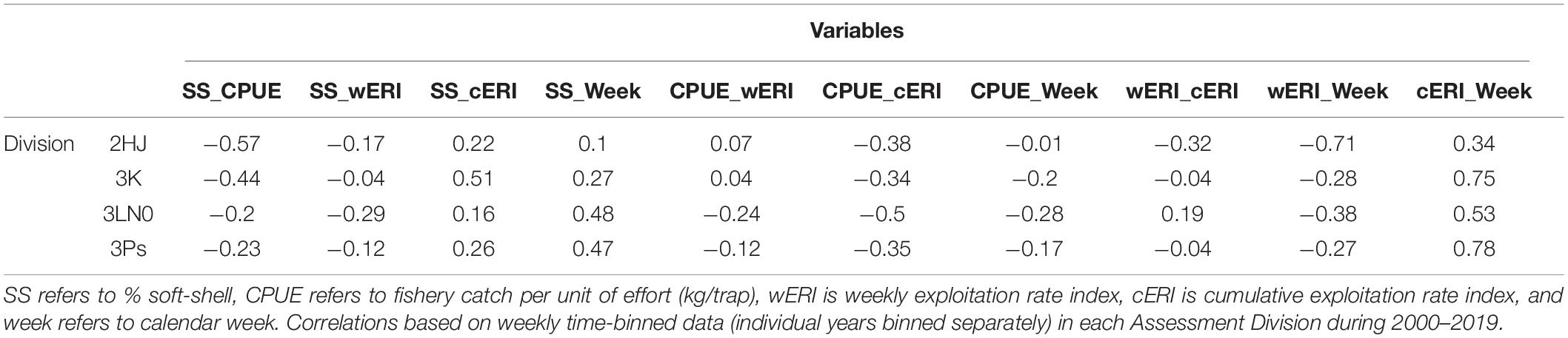
Table 1. Pearson correlation of exploratory explanatory variables considered for modeling soft-shell crab prevalence.

Week and cERI were positively correlated in each AD (r: 0.34–0.78) (Table 1). However, a pattern of progressively higher levels of cERI occurring earlier in the year occurred in each AD over the time series (Figure 2). There was also contrast in fishery duration across ADs. Since 2010, the AD 3Ps fishery has not regularly progressed past June, or even May, while the fishery typically extended into July in the other ADs. These within- and across-AD differences in fisheries exploitation patterns and associated levels of SS prevalence were deemed to provide sufficient contrast to partially offset concerns of collinearity among the two explanatory variables in hGAMM predictive modeling.

FIGURE 2

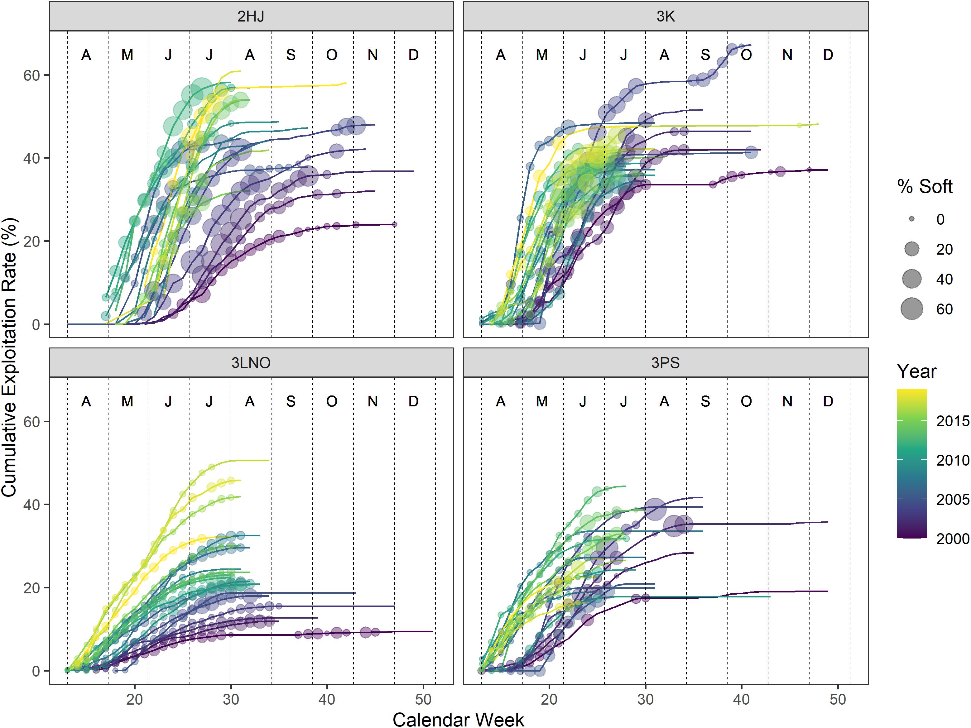
Figure 2. Percentages of soft-shell crab sampled in the catch versus cumulative exploitation rates in the fishery by week during 2000–2019. Weeks without a soft-shell observation denote weeks where no sampling occurred. Vertical dashed lines segregate months, which are denoted by the alphabet symbols near the top of each panel (A=April, D=December).

SS crab percentages in the catch generally increased as both cERI and calendar week increased in all ADs (Figure 2). Overall contrast in harvesting strategies occurred across ADs, with ADs 2HJ and 3K frequently harvesting at rates of 40–60% cERI in any given year, while ADs 3LNO and 3Ps more frequently remained below 40% cERI. Overall highest levels of SS crab in the fishery occurred in ADs 2HJ and 3K where weekly observations above 20% were common.

Predictive Modeling

The hGAMM showed that group-level interactions of week and cERI were significant (p < 0.0001) predictors of percentage of SS crab in the fishery in all but AD 3LNO (Table 2). Moreover, the global-level interaction of these two variables exerted some (albeit weak) statistical influence in the process (p = 0.075). The interaction of year and AD was significant (p < 0.0001). Overall, the model explained 79.2% of the deviance in the process of weekly SS crab incidence in fishery (adj. r² = 0.63).

TABLE 2

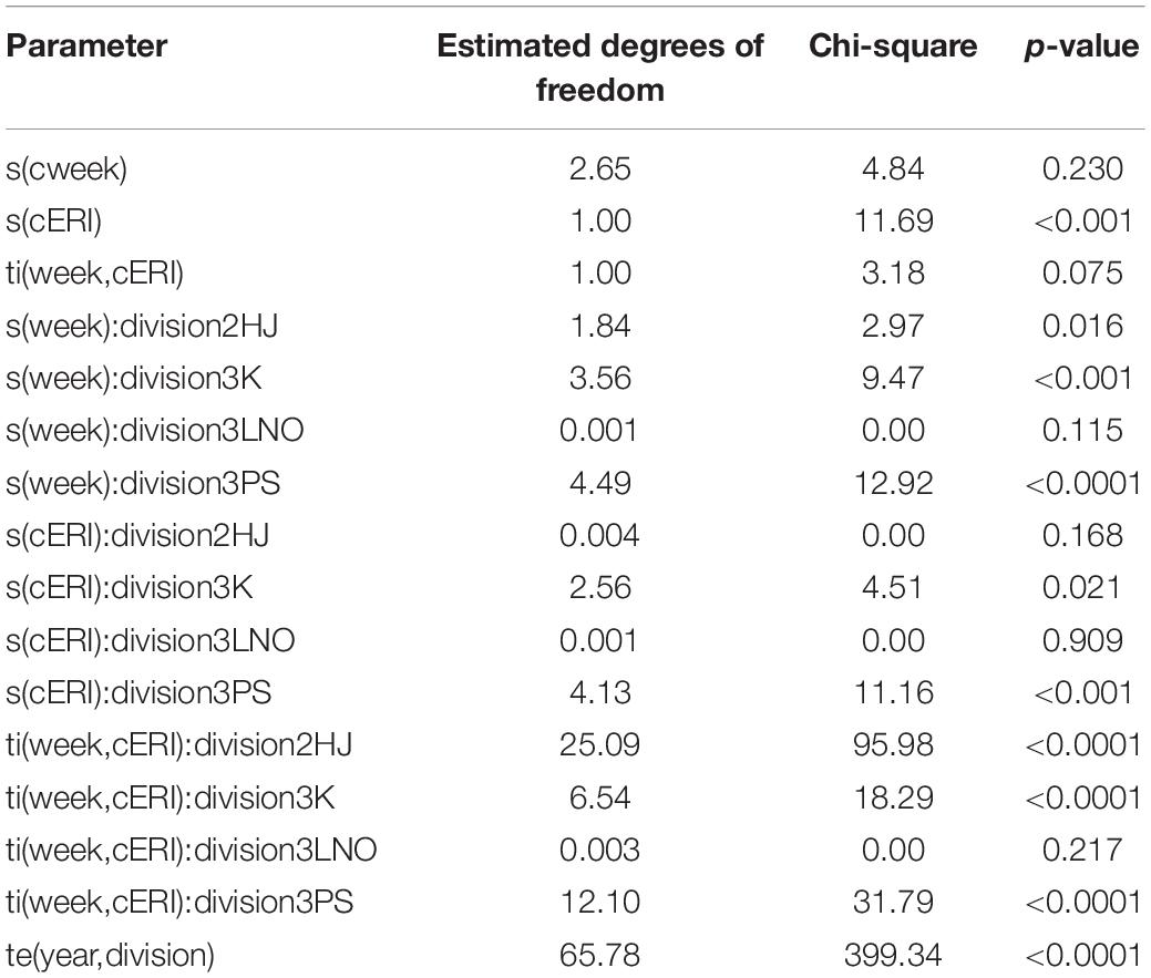
Table 2. Output of hierarchical generalized additive mixed model on factors affecting soft-shell crab levels in the NL snow crab fishery.

The model was able to fit weekly SS proportion data well in most ADs and years (Supplementary Figure 2). However, there was a directionally systematic occurrence of model inability to capture sporadic and unusually high weekly SS estimates. Accordingly, model predictions of SS incidence are likely slightly underestimated. A particularly evident pattern of poor model fit in the form of underestimation in AD 2HJ during 2002–2004 is attributable to data anomalies resulting from unusually high levels of exploitation and changed fishery practices following establishment of an exclusive fishing area in that AD as described in Mullowney et al. (2012).

The marginal effect smooths showed both consistency and differences in how cERI and week affected SS incidence in the fishery across ADs (Figure 3). In ADs 2HJ and 3K, SS percentage quickly increased with exploitation pressure, initially reaching SS Protocol closure thresholds of 15% after about 20% (2HJ) or 30% (3K) of the biomass was removed. In the more lightly exploited ADs 3LNO and 3Ps, the effect of cERI was not easily described (3Ps) or negligible (3LNO) in regulating SS prevalence in the fishery. Temporally, earlier and overall greater levels of peak SS levels occurred in ADs 2HJ (peak at week 25) and 3K (peak at week 27). The results suggest the SS Protocol closure threshold of 15% would typically be reached by late-May or early June in these ADs. Peak SS incidence in the AD 3LNO fishery occurred in week 30 (end of July or early August) at a level of 10%. Finally, there was no consistent directional effect of week on SS incidence in AD 3Ps until the latest stages of the fishery, with estimates of SS ranging from 10 to 14% of the catch from weeks 34 (late August) onward.

FIGURE 3

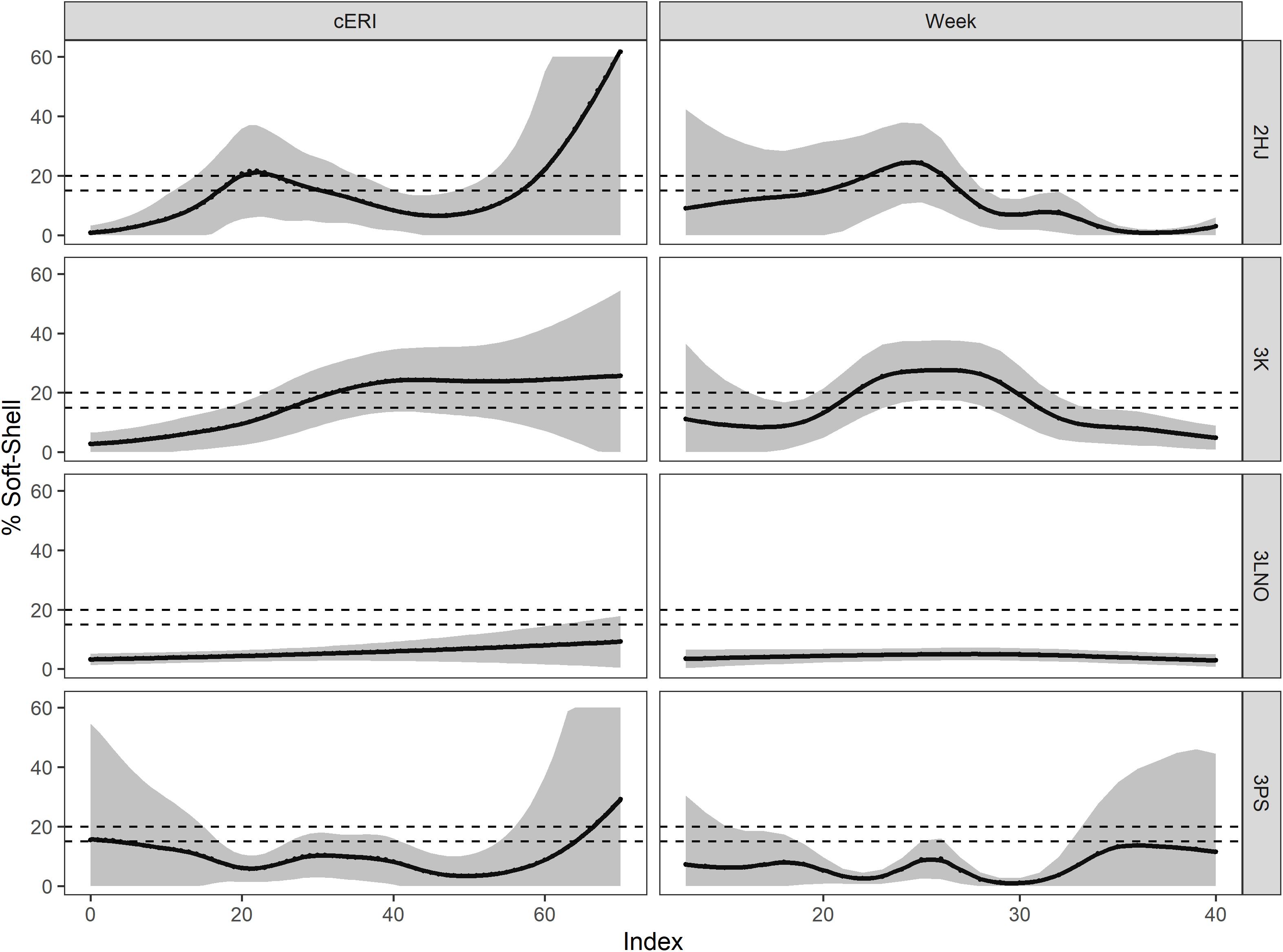
Figure 3. Marginal smooths for main effects of cumulative exploitation rate (cERI, left panels) and calendar week (Week, right panels) in affecting soft-shell prevalence in the fishery during 2000–2019, by Assessment Division. Dashed horizontal lines show management closure thresholds for soft-shell crab in the fishery (15% in AD 3LNO and 20% in ADs 2HJ, 3K, and 3Ps). Shaded areas show 95% prediction intervals.

Relevant Management Information

Shell condition histories of the catch in ADs 3LNO and 3Ps showed relatively little reliance on immediate recruitment in the fishery, with the weekly catch consistently dominated by old-shell crab (typically ≥ 60% of the weekly catch) (Figure 4). In contrast, in ADs 2HJ and 3K, old-shell crab ranged about 40–50% of the catch in most weeks prior to August, after which new-shell crab increased in importance and dominated the catch by September. There was a strong signal of SS crab in June and July catches in ADs 2HJ and 3K (i.e., up to 30% of the weekly catch) from June-August, with little indication of SS incidence in the AD 3LNO catch overall or until August in AD 3Ps.

FIGURE 4

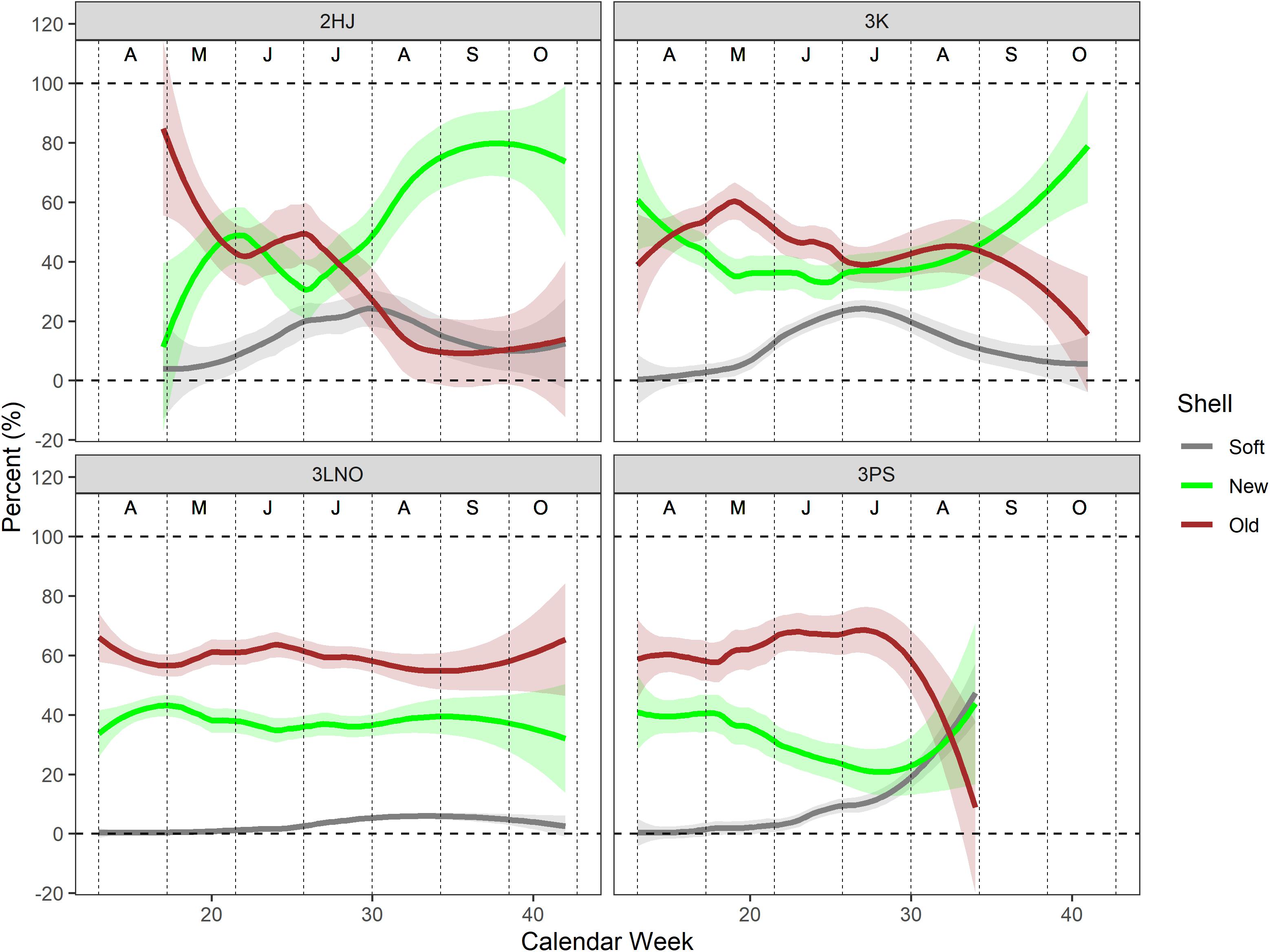
Figure 4. Loess regression curves of shell type composition in the weekly catch during the 2000–2019 period. All years of data pooled. Shaded bands are 95% confidence intervals. Vertical dashed lines segregate months, which are denoted by the alphabet symbols near the top of each panel (A=April, D=December).

Surplus fishing mortality stemming from soft-shell handling was low under both high (90%) and low (10%) assumed mortality rates throughout the time series in ADs 3LNO and 3Ps (Supplementary Figure 3). However, there have been consistently higher levels of unaccounted for surplus mortalities in the ADs 2HJ and 3K fisheries. Although these annual potential surplus mortality levels are typically below 10% of the landings, in extreme cases where the overall percentage of SS crab in the catch is high and a high discard mortality rate (90%) is assumed, wastage levels could elevate to 15–35% of the landings and amounted to maximums of ≥ 1,000 and 5,000 t of crab in ADs 2HJ and 3K, respectively, during the 2000–2005 period. The analysis suggests it is likely that exploitation rates in the ADs 2HJ and 3K fisheries have been consistently under-estimated, and could have realistically been an additional 5–15% higher than the reported index in most years, operating under an assumption of a medium (50%) level of mortality on discarded SS crab.

Temperature-at-capture versus estimated peak SS timing revealed a strong directional trend toward earlier SS incidence associated with fisheries occurring in warmer areas (Figure 5). Males best representing pre-recruits and recruits were captured in warmest waters in AD 2HJ (mean of 3.02°C) and coldest waters in AD 3Ps (mean of 0.24°C). These temperature extremes were associated with peak fishery SS periods of weeks 25 and 36, respectively, an 11 week difference. This 3 months difference suggests the phenomenon is not likely to be fully attributable to potential confounds of differences in exploitation or survey timing across ADs. This assertion is supported by the similar capture temperatures for the crab in the spring (mean of 1.37°C) and fall (mean of 0.99°C) surveys in AD 3LNO.

FIGURE 5

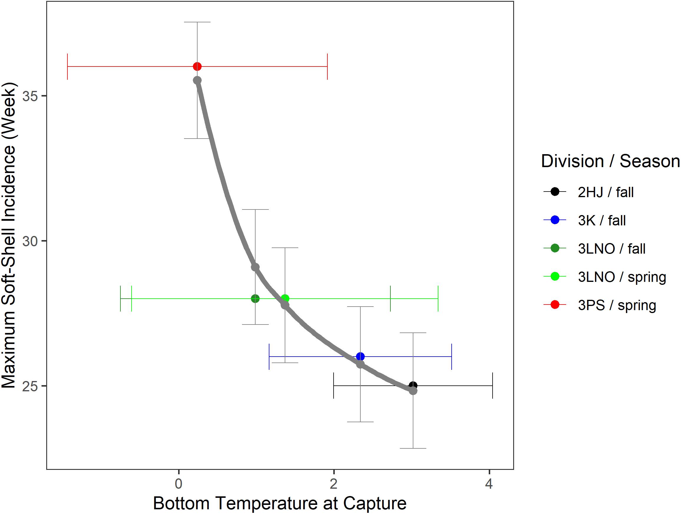
Figure 5. Calendar week of peak incidence of soft-shell crab in the fishery estimated from hGAMM [1] versus bottom temperature of capture during DFO fall or spring research bottom trawl surveys for pre-recruit or recruit crab in the exploitable biomass. Data pooled over the time series within each Assessment Division and season-specific survey series. Horizontal error bars are one standard deviation of temperature away from the mean point-estimate. Solid gray curve is a log-log regression line. Vertical error bars are 95% confidence intervals of maximum soft-shell prevalence week in the fishery estimated from the regression model.

Discussion

Biology of Soft-Shell Crab

This study confirms previous suggestions that seasonality and fisheries exploitation rates are key processes affecting prevalence of SS incidence in snow crab fisheries (e.g., Mullowney et al., 2019). However, the study importantly extends upon this by demonstrating interactions between the two factors in regulating fishery SS levels. The study also advances knowledge on the impacts of temperature on molt-timing in wild populations, supporting previous tank-based observations of earlier molting under warm conditions (Dutil et al., 2010).

In warm areas such as ADs 2HJ and 3K, the peak timing of SS is during late spring or early summer (June–July), while in colder areas (ADs 3LNO and 3Ps) it occurs during summer or early fall (July–September). The phenology of SS incidence is an uncontrollable natural process while fisheries exploitation is a controllable anthropogenic process and evidence shows that despite varying ecological processes, stringent control of fisheries exploitation rates can consistently minimize soft-shell incidence in the catch. The comparative analysis shows that under light to moderate levels of fisheries exploitation (∼30% of the available exploitable biomass) the fishery can normally be prosecuted with relatively low levels of SS in the catch (<15%), even during peak SS periods. Under heavier levels of exploitation, higher incidences of SS crab in the catch are likely to occur.

The anthropogenic perturbation of fisheries exploitation directly affects the biological process of intraspecific competition. As per Mullowney et al. (2019), the present results suggest increased SS crab catchability is associated with competition release stemming from depletion of the residual biomass of large hard-shell males in the population. The impacts of high levels of fisheries exploitation in ADs 2HJ and 3K have long been cited as a biological concern (Mullowney et al., 2012, 2019, 2020). Globally, few other snow crab fisheries consistently harvest the exploitable biomass as heavily as historically fished in ADs 2HJ and 3K (Mullowney et al., 2019, 2020), and biological problems from chronically depleting the residual biomass are becoming increasingly obvious (Mullowney et al., 2020).

Issues of excessive exploitation promoting high incidences of SS crab in a fishery are not exclusive to snow crab. Smith and Jamieson (1989) previously demonstrated this phenomenon in a fishery for dungeness crab (Cancer majister) in British Columbia. Following the definition of recruitment in Ricker (1975), with recruitment referring to animals first contributing to the fishery, SS crab incidence serves as a direct indicator of recruitment overfishing in exploited snow crab resources. The philosophy of recruitment overfishing can be extended to discard or retention of new-shell crab if they are captured in the year of molt because they render less than optimal levels of meat fullness (Mullowney et al., 2020) and necessitate more crab to be extracted to fulfill given quota allocations.

SS crab constitutes, to some degree, the sacrifice of next year’s catch in lieu of catch in the present. Given direct and strong negative correlations between SS incidence and fisheries CPUE, this act of recruitment overfishing is often associated with little to no gain in the fishery in the present.

The problem of SS incidence in the fishery becomes circular under persistently excessive exploitation as the population cannot sufficiently recover from one fishing season to the next. For example, an incoming pulse of recruitment strong enough to promote resource recovery requires several years to become firmly established as a residual biomass because variable portions of each cohort follow a multinomial process of either molting to adolescence, terminally molting, or skip-molting in a given year; complicating annual harvest strategies for fisheries management.

Management of Soft-Shell Crab

The most general management advice to emerge is that late-spring to early fall is a poor time to fish snow crab if the harvest strategy is to heavily exploit the resource. Despite habitat-related differences in peak timing of SS incidence, the contrast among ADs lead to an obvious analytical outcome demonstrating that snow crab fisheries “can’t have it both ways” with respect to high exploitation rates and a summer seasonality. We suggest a level of 30% annual exploitation rate as a guiding measure if minimization of soft-shell crab is to be a focal priority in spring to fall fisheries, either in NL or elsewhere. This is based primarily on the historic success of AD 3LNO fisheries.

Our analysis demonstrates general factors that control levels of soft-shell crab incidence in the fishery (harvest levels and seasonality) across heterogeneous environments but also highlights AD-specific differences in temporal patterns of soft-shell timing associated with temperature conditions. In similar fashion, contrasting management strategies across ADs could also affect outcomes. Two of the main management strategies instituted into the fishery in any given AD and year are exploitation rates and seasonality. These decisions are implemented through a co-management process (Mullowney et al., 2020) and AD-specific factors such as differences in harvester risk tolerance or fishery dependency could plausibly affect decisions on exploitation levels while factors such as sea ice coverage could affect decisions on seasonality. Of the two major processes highlighted, exploitation rate has been the more variable across ADs. A systematic push toward earlier fishing seasons has occurred in all ADs throughout the time series and despite a consistent pattern of the southern AD (ice-free) fisheries occurring earlier, there is a core period during which fisheries in all ADs overlap in any given year. This core period corresponds to April to June for most of the past decade. Accordingly, exploitation rates are overall the more dynamic process of consciously controllable management factors affecting outcomes of soft-shell incidence in the fishery.

The SS Protocol is intended to safeguard against SS mortality in the fishery (DFO., 2020). However, the scientific assessment has long expressed concerns that the SS Protocol is ineffective due to too many grid cells and too little observer coverage, among other issues. In most areas and years a given cell has a 0–25% chance of being monitored for potential closure (Mullowney et al., 2020), operating under a best-case scenario that it need only be visited once during the season. Beyond issues of low observer coverage, the spatiotemporal differences in fishery SS timing shown herein further compound the shortcomings of the SS Protocol as they confirm the necessity to frequently monitor grid cells throughout the season to accurately quantify SS incidence.

Two of the largest global fisheries for snow crab have occurred in NL and Alaska over the past three decades. The Alaska fishery primarily occurs during winter. Contrast among the two fisheries in context of stock composition in relation to optimal fishery timing offers intriguing management theory insights. Beyond increased SS wastage in NL summer fisheries, extraction efficiency of new-shell crab is important to consider. Over the past decade both stocks consistently show a dominance of new-shell crab in the exploitable population at either the stock level (Alaska, Lang et al., 2018) or in sub-component units of the stock (NL, Mullowney et al., 2019). As new-shell crab are not guaranteed to be filled with meat until December (Mullowney et al., 2020), it is more efficient to harvest them over-winter or in the subsequent spring, as opposed to the summer or even fall of their current molt year.

Alaska is more easily able to harvest snow crab during winter due to a different management/fishery system featuring large vessels and a small fleet size (i.e., dozens of vessels) as opposed to a small vessel large fleet size model in NL (Mullowney et al., 2020). In both regions, annual ice coverage would normally be at its maximum extent during early spring (i.e., about March) and therefore have maximum potential to interfere with early spring fisheries. From a biological stance, early spring fisheries would also theoretically have a high potential to interfere with mating periods of both primiparous (over-winter) and multiparous (early spring) females whereas concerns of winter fishing on mating processes would be more exclusive to the primiparous mating period. With respect to mortality rates in soft-shell discarded crab in relation to air temperatures, both winter and summer seasons have been shown to be problematic for discard mortality in snow crab, with both extreme cold (van Temelen, 2005; Urban, 2015) and warm (Dufour et al., 1997) conditions associated with higher mortality rates than more temperate conditions.

Ultimately, optimal fishery timing must coincide with socio-political factors in a fisheries management system. Given the reality that the biologically-optimal harvest time of winter or early spring (periods associated with little to no soft-shell crab in the catch) is a challenge for the small-boat fisheries, a best-advised management strategy for such circumstances is to focus on consistently maintaining a high residual biomass of large hard-shell males in the population at all times. This strategy is readily enabled through persistent low exploitation rates.

Conclusion

The study concludes that seasonality and fisheries exploitation rates interact to govern levels of soft-shell crab incidence in snow crab fisheries. Highest potential for elevated soft-shell incidence to occur in snow crab fisheries is during late-spring or early summer (June–July) in warm areas subjected to high exploitation rates. Despite providing novel evidence on how habitat regimes may affect molt timing in wild snow crab populations, we promote a consistently applicable best-practice management recommendation that an extraction strategy of maintaining low exploitation rates and a high residual biomass in the population at all times will minimize fishery soft-shell encounters in all areas. This strategy is particularly relevant when fisheries cannot be conducted during winter, which we affirm as the most optimal time to harvest snow crab from both biological and extraction efficiency perspectives. Strong residual biomasses of large hard-shell males promote sufficient intraspecific competition to minimize soft-shell incidence in the fishery, even during peak soft-shell periods. Finally, we conclude that spatiotemporal variation in molt-timing further complicates in-season monitoring abilities for programs such as the SS Protocol instituted in management of the NL and other Atlantic Canadian snow crab fisheries to meet objectives of controlling handling mortality.

Data Availability Statement

The data analyzed in this study is subject to the following licenses/restrictions: The Government of Canada is striving to make data publicly available. In the meantime the data can be made available by the authors upon reasonable request. Requests to access these datasets should be directed to JP, Julia.Pantin@dfo-mpo.gc.ca.

Author Contributions

DM, KB, and JP conceived the study and undertook the formal analysis. DM drafted the manuscript. KB and JP reviewed and edited the manuscript. All authors contributed to the article and approved the submitted version.

Conflict of Interest

The authors declare that the research was conducted in the absence of any commercial or financial relationships that could be construed as a potential conflict of interest.

Acknowledgments

We express much respect and appreciation to the team of fisheries observers from SeaWatch in St. John’s, NL, who have collected the data on snow crab shell condition and sizes used in this study. We also express thanks to the DFO technical staff from Science Branch in St. John’s, NL who have collected and compiled survey information used in this analysis as well as screened and edited observer data on our behalf. The study received two constructive reviews by Katherine Skanes and Hannah Murphy prior to submission, with our thanks extended to both for their perspectives and comments. Finally, we thank Eric Pedersen for advanced insights into hierarchical Generalized Additive Modeling in R.

Supplementary Material

The Supplementary Material for this article can be found online at: https://www.frontiersin.org/articles/10.3389/fmars.2021.591496/full#supplementary-material

Supplementary Image 1 | Percent of fishery catch observed (top panel) and measured (bottom panel) by at-sea observers for each Division from 2000-2019.

Supplementary Image 2 | Observed versus hGAMM-predicted values for proportions of the catch the were soft-shell by Division and year. Points represent weekly values. Slanted lines denote a 1:1 relationship.

Supplementary Image 3 | Estimates of surplus fishing mortality associated with capture and discard of soft-shell crab by Division and year. Coloured lines indicate low (10%) to high (90%) mortality scenarios. Left panels show surplus mortality above reported landings by tonnage and right panels show surplus mortality above reported landings by exploitation rates.

References

Burmeister, A. D., and Sainte-Marie, B. (2010). Pattern and causes of a temperature-dependent gradient of size at terminal moult in snow crab (Chionoecetes opilio) along west greenland. Polar Biol. 33, 775–788. doi: 10.1007/s00300-009-0755-6

CrossRef Full Text | Google Scholar

Comeau, M., Robichaud, G., Starr, M., Therriault, J.-C., and Conan, G. (1998). Mating of snow crab (Chionoecetes opilio, O. Fabricius 1788) (decapoda, majidae) in the fjord of bonne bay, newfoundland. Crustaceana 71, 925–941. doi: 10.1163/156854098x00932

CrossRef Full Text | Google Scholar

Cyr, F., Colbourne, E., Galbraith, P. S., Gibb, O., Snook, S., Bishop, C., et al. (2020). Physical oceanographic conditions on the newfoundland and labrador shelf during 2018. DFO Can. Sci. Advis. Sec. Res. Doc. 2020:48.

Google Scholar

Dawe, E. G., and Colbourne, E. B. (2002). “Distribution and Demography of Snow Crab (Chionoecetes opilio) Males on the Newfoundland and Labrador Shelf,” in Crabs in Cold Water Regions: Biology, Management, and Economics, eds A. J. Paul, E. G. Dawe, R. Elner, G. S. Jamieson, G. H. Kruse, R. S. Otto, et al. (Fairbanks, Alaska: Alaska Sea Grant College Program, University of Alaska), 577–594.

Google Scholar

Dawe, E. G., Mullowney, D. R., Moriyasu, M., and Wade, E. (2012). Effects of temperature on size-at-terminal molt and molting frequency in snow crab Chionoecetes opilio from two canadian atlantic ecosystems. Mar. Ecol. Prog. Ser. 469, 279–296. doi: 10.3354/meps09793

CrossRef Full Text | Google Scholar

DFO. (2020). Snow Crab Integrated Management Plan. Available Online at: http://www.dfo-mpo.gc.ca/fisheries-peches/ifmp-gmp/snow-crab-neige/2019/index-eng.htm. [Accessed May 13, 2020]

Google Scholar

Dufour, R., Bernier, D., and Brêthes, J.-C. (1997). Optimization of meat yield and mortality during snow crab (Chionoecetes opilio O. Fabricius) fishing operations in eastern canada. Can. Tech. Rep. Fish. Aquat. Sci. 2152, 30.

Google Scholar

Dutil, J.-D., Dion, C., Gamache, D. L., Larocque, R., and Ouellet, J.-F. (2010). Ration and temperature effects on the condition of male adolescent molter and skip molter snow crab. J. Shellfish Res. 29, 1025–1033. doi: 10.2983/035.029.0404

CrossRef Full Text | Google Scholar

Grant, S. M. (2003). Mortality of snow crab discarded in newfoundland and labrador’s trap fishery: at-sea experiments on the effect of drop height and air exposure duration. Can. Tech. Rep. Fish. Aquat. Sci. 2481:28.

Google Scholar

Kolts, J. M., Lovvorn, J. R., North, C. A., and Janout, M. A. (2015). Oceanographic and demographic mechanisms affecting population structure of snow crabs in the northern bering sea. Mar. Ecol. Prog. Ser. 518, 193–208. doi: 10.3354/meps11042

CrossRef Full Text | Google Scholar

Lang, C. A., Richar, J. I., and Foy, R. J. (2018). The 2017 eastern bering sea continental shelf and northern bering sea bottom trawl surveys: results for commercial crab species. U.S. department of commerce. NOAA Tech. Memo. NMFS-AFSC 372:233.

Google Scholar

Miller, R. J. (1977). Resource underutilization in a spider crab industry. Fisheries 2, 9–13. doi: 10.1577/1548-8446(1977)002<0009:ruiasc>2.0.co;2

CrossRef Full Text | Google Scholar

Mullowney, D., Baker, K., Coffey, W., Pedersen, E., Colbourne, E., Koen-Alonso, M., et al. (2019). An assessment of newfoundland and labrador snow crab (Chionoecetes opilio) in 2017. DFO Can. Sci. Advis. Sec. Res. Doc. 2019:172.

Google Scholar

Mullowney, D., Morris, C., Dawe, E., Zagorsky, I., and Goryanina, S. (2018a). Dynamics of snow crab (Chionoecetes opilio) movement and migration along the newfoundland and labrador and eastern barents sea continental shelves. Rev. Fish Biol. Fish. 28, 435–459. doi: 10.1007/s11160-017-9513-y

CrossRef Full Text | Google Scholar

Mullowney, D., Baker, K., Pedersen, E., and Osborne, D. (2018b). Basis for a precautionary approach and decision making framework for the newfoundland and labrador snow crab (Chionoecetes opilio) fishery. DFO Can. Sci. Advis. Sec. Res. Doc. 2019:66.

Google Scholar

Mullowney, D. R. J., Baker, K. D., Zabihi-Seissan, S., and Morris, C. (2020). Biological perspectives on complexities of fisheries co-management: a case study of newfoundland and labrador snow crab. Fish. Res. 232:105728. doi: 10.1016/j.fishres.2020.105728

CrossRef Full Text | Google Scholar

Mullowney, D. R. J., Morris, C. J., Dawe, E. G., and Skanes, K. R. (2012). Impacts of a bottom trawling exclusion zone on snow crab abundance and fish harvester behavior in the labrador sea, canada. Mar. Policy 36, 567–569. doi: 10.1016/j.marpol.2011.10.005

CrossRef Full Text | Google Scholar

Pedersen, E. J., Miller, D. L., Simpson, G. L., and Ross, N. (2019). Hierarchical generalized additive models in ecology: an introduction with mgcv. PeerJ. 7:e6876. doi: 10.7717/peerj.6876

PubMed Abstract | CrossRef Full Text | Google Scholar

R Core Team. (2019). R: A language and environment for statistical computing. Vienna, Austria: R Foundation for Statistical Computing.

Google Scholar

Ricker, W. E. (1975). Computation and interpretation of biological statistics of fish populations. Bull. Fish. Res. Board Can. 191:382.

Google Scholar

Sainte-Marie, B., Dionne, H., and Alarie, M.-C. (2010). “Temperature and Age Dependent Fertile Period in Female Snow Crab (Chionoecetes opilio) at the Maturity Molt,” in Biology and Management of Exploited Crab Populations under Climate Change, eds G. H. Kruse, G. L. Eckert, R. J. Foy, R. N. Lipcius, B. Sainte-Marie, D. L. Stram, et al. (Fairbanks, Alaska: Alaska Sea Grant, University of Alaska Fairbanks), 217–235.

Google Scholar

Sainte-Marie, B., and Hazel, F. (1992). Moulting and mating of snow crabs, Chionoecetes opilio (O Fabricius), in shallow waters of the northwestern gulf of St Lawrence. Can. J. Fish. Aquat. Sci. 49, 1282–1293. doi: 10.1139/f92-144

CrossRef Full Text | Google Scholar

Sainte-Marie, B., Urbani, N., Hazel, F., Sévigny, J. M., and Kuhnlein, U. (1999). Multiple choice criteria and the dynamics of assortative mating during the first breeding season of the female snow crab Chionoecetes opilio (brachyura, majidae). Mar. Ecol. Prog. Ser. 181, 141–153. doi: 10.3354/meps181141

CrossRef Full Text | Google Scholar

Smith, B. D., and Jamieson, G. S. (1989). Exploitation and mortality of male dungeness crabs (Cancer majister) near tofino, british colombia. Can. J. Fish. Aquat. Sci. 46, 1609–1614. doi: 10.1139/f89-205

CrossRef Full Text | Google Scholar

Urban, J. D. (2015). Discard mortality rates in the bering sea snow crab (Chionoecetes opilio) fishery. ICES J. Mar. Sci. 72, 1525–1529. doi: 10.1093/icesjms/fsv004

CrossRef Full Text | Google Scholar

van Temelen, P. G. (2005). Estimating handling mortality due to air exposure: development and application of thermal models for the bering sea snow crab fishery. Trans. Am. Fish. Soc. 134, 411–429. doi: 10.1577/t04-091.1

CrossRef Full Text | Google Scholar

Wood, S. N. (2006). Low rank scale invariant tensor product smooths for generalized additive mixed models. Biometrics 62, 1025–1036. doi: 10.1111/j.1541-0420.2006.00574.x

PubMed Abstract | CrossRef Full Text | Google Scholar

Wood, S. N. (2011). Fast stable restricted maximum likelihood and marginal likelihood estimation of semiparametric generalized linear models. J. R. Stat. Soc. (B) 73, 3–36. doi: 10.1111/j.1467-9868.2010.00749.x

CrossRef Full Text | Google Scholar

Wood, S. N. (2017). Generalized Additive Models: An Introduction with R (2nd edition). Boca Raton, London. New York: CRC Press.

Google Scholar