Short-Term Spatiotemporal Variability in Picoplankton Induced by a Submesoscale Front South of Gran Canaria (Canary Islands)

Introduction

As higher plants, unicellular marine primary producers’ growth mainly depends on nutrient and light availability. Access to these resources may be limited in the highly dynamic oceanic environments, which are dominated by physical processes that generally alter resource availability. Indeed, a large amount of studies has indicated that the distribution and variability of phytoplankton and other biogeochemical parameters like nutrients and organic matter in the upper layers of the ocean are highly correlated in time and space with physical processes (Abraham, 1998; Mahadevan and Campbell, 2002; Lévy and Klein, 2004; Niewiadomska et al., 2008; Omta et al., 2008; Lehahn et al., 2017).

Mesoscale motions have commonly been assumed to be the most important factor modulating the distribution of biogeochemical properties at the upper levels of the ocean (Falkowski et al., 1991; Oschlies and Garçon, 1998; McGillicuddy et al., 2007; Johnson et al., 2010). However, recent theoretical studies (Lévy et al., 2001; Mahadevan and Campbell, 2002; Mahadevan and Tandon, 2006; Klein and Lapeyre, 2009) have highlighted the role played by smaller processes that operate below the local Rossby radius of deformation, referred to here as submesoscale. An estimated 50% of the total variance of vertical velocities in the upper layer of the ocean may be explained by submesoscale processes (Klein and Lapeyre, 2009). These small-scale motions arise from the disruption of the geostrophic balance by mesoscale straining being common in fronts and eddies edges. Vertical motions associated with ageostrophic secondary circulation (ASC) are originated at both sides of the fronts (upward on the warm side and downward on the cold side) leading to small-scale fluxes of biogeochemical properties like nutrients (Mahadevan and Tandon, 2006; Lévy et al., 2012a). Diapycnal mixing has been shown to be a dominant component of the vertical velocity in submesoscales fronts and filaments by destroying the thermal wind and driving intense ASC in the upper layers (Estrada-Allis et al., 2019). Thus, intensification of diapycnal mixing may enhance vertical transport of nutrients (Arcos-Pulido et al., 2014; Corredor-Acosta et al., 2020; Tsutsumi et al., 2020) as well as upwelling/downwelling of phytoplankton communities from sub-surface layers into the euphotic zone and vice versa. These physical cells act to restore the geostrophy by means of restratification in a process known as frontogenesis (Hoskins and Bretherton, 1972; Hoskins, 1982; Capet et al., 2008; McWilliams, 2016). The importance of submesoscale lies in that their spatiotemporal scales are similar to those in which biological process acts, i.e., from 0.1 to tens of kilometers and of the order of 0 (1–10) days. Phytoplankton productivity and growth may thus be influenced by those changes in nutrient and light availabilities (Allen et al., 2005; Lévy et al., 2009, 2018; Lathuiliere et al., 2011; Taylor and Ferrari, 2011; Shulman et al., 2015; Liu and Levine, 2016; Taylor, 2016; Hosegood et al., 2017). Additionally, submesoscale motions may also induce shifts on phytoplankton community structure (D’Ovidio et al., 2010; Lévy et al., 2018) affecting food web dynamics and, ultimately, the carbon cycle (Mayot et al., 2017).

The study of the mechanisms controlling frontogenesis and the associated ASC is a relevant topic due to its potential impact, not only on the short-term modulation of nutrients, organic matter or light, and hence on phytoplankton communities (Mahadevan and Campbell, 2002; Klein and Lapeyre, 2009; Lévy et al., 2009, 2012a), but also because of its role in example global ocean circulation (D’Asaro et al., 2011; Taylor and Ferrari, 2011; Lévy et al., 2012b), heat transport (Siegelman et al., 2020) or fish and marine mammal distribution (Snyder et al., 2017; Siegelman et al., 2020). However, due to the inherent complexity of sampling at such high-resolution levels, only a few studies have reported in situ data of submesoscale spatial phytoplankton distribution across a frontal region yet (e.g., Martin et al., 2005; Taylor et al., 2012; Clayton et al., 2014; Cotti-Rausch et al., 2016; Mousing et al., 2016; Hernández-Hernández et al., 2020). Therefore, our knowledge about submesoscale-influenced phytoplankton distribution and variability mostly constrained to the information extracted from theoretical and modeling studies (Lévy et al., 2001, 2012a; Li et al., 2012; Liu and Levine, 2016; Taylor, 2016).

In this study, we provide physical and biogeochemical observations on the development and decay of a submesoscale wind-shear front formed on the wake of Gran Canaria Island. Our overarching objective is to discuss how short-term front-generated physical variability affects the distribution and community structure of picophytoplankton organisms, which are major contributors to total phytoplankton biomass and primary production in the subtropical waters surrounding the Canary archipelago (Zubkov et al., 2000a,b; Arístegui et al., 2009). For that aim, we first study the spatiotemporal evolution of the front and biogeochemical parameters. We then statistically examine the effect of the front over the phytoplankton distribution and community structure via Metric Multidimensional Scaling Analysis. We finally compare the variance induced by the spatial and temporal variabilities to determine which source of variability has major influence over picoplankton community variability.

Materials and Methods

Hydrography, Wind and Sampling Design

Data reported in this paper were collected from 9 to 12 of May of 2011 on board R/V Atlantic Explorer from a section across a wind-shear convergent front (Figures 1a,b). In order to assess both spatial and temporal variability at submesoscale range [horizontal scale of O (1–10 km), vertical scale of O (100 m) and temporal scale of O (1 day)], a section consisting in 6–7 oceanographic stations (Figures 1a,b), separated ∼4 km (25 km in total), was entirely sampled every 24 h, during a 96 h period. Unfortunately, intense wind speed (Figure 1c) did not allow the sampling of the section at 48 h (May 11th). At each station, conductivity-temperature-depth (CTD) casts were made from surface to 300 m using a SeaBird SBE25 CTD sensor additionally equipped with a Wet Lab ECO-AFL/FL Fluorometer. The CTD was mounted onto an oceanographic rosette implemented with six Niskin bottles of 12 L. Discrete water samples were collected for chlorophyll a (Chl a), nutrients and picophytoplankton abundances at six levels, from surface to 150 m, including the deep chlorophyll maximum (DCM). TEOS-10 algorithms were used to calculate all physical derived variables. Mixed layer depth (MLD) was calculated following (de Boyer Montégut et al., 2004). Wind velocities and directions every 10 min were obtained from the Meteorological Station based on the Gando Airport, at the wind-exposed eastern coast of the Gran Canaria Island. Raw wind data was averaged every 4 h for plotting (Figure 1c).

FIGURE 1

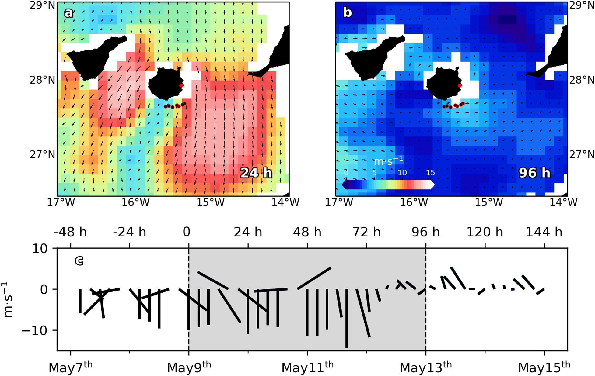
Figure 1. Sea surface winds (m⋅s^{– 1}) and direction (black arrows) from scatterometer on the Meteorological Operational satellite MetOp-A (European Space Agency, ESA), for (a) May 10th 2011 (24 h) and (b) May 13th 2011 (96 h). Black dots with red borders indicate stations positions. Red dot indicates Gando airport location. (c) Wind speed (m⋅s^{– 1}) time series from May 7th to May 15th. Dashed vertical lines delimit sampling period. Negative (positive) values correspond with north (south) and east (west) wind directions.

Satellite-Derived Data

Satellite-derived wind velocities and directions components displayed in Figures 1a,b were obtained from the scatterometer mounted on the polar-orbiting satellite MetOp-A (Meteorological Operational satellite) of the European Space Agency (ESA) and provided by Copernicus Marine Environment Monitoring Services (CMEMS). Sea surface temperature (SST) and salinity (SSS) from the CMEMS’s product, Atlantic -Iberian Biscay Irish- Ocean Physics Reanalysis accessible through https://resources.marine.copernicus.eu, was used to track the frontal evolution during the cruise. Both data sets present daily temporal resolution, while offering a horizontal resolution of 12.5 × 12.5 km and 8 × 8 km for wind and temperature and salinity, respectively.

Vertical Motions

Vertical velocities associated with diapycnal mixing were calculated under the assumption of negligible viscous forces and important rotation effects. In this case, the ageostrophic Coriolis forcing can be balanced by vertical mixing, and it holds by the scaling of Garret and Loder (1981), w_GL hereinafter:

$$w_{GL}\sim \frac{-1}{{\mathrm{\rho }}^2}\frac{\partial }{\partial x}(A_{\text{v}}\frac{\partial b}{\partial x})$$

where x is the cross-frontal direction, A_v is the vertical eddy viscosity, and b is the buoyancy in terms of density (ρ), mean density (ρ_o), and gravitational acceleration (g), such as b = −g (ρ/ρ_o).

Though vertical velocities from w_GL must not be taken as total vertical velocity, it allows us to compare the magnitude of the diffusive flux and vertical advective flux, i.e., the magnitude of the vertical velocity due diapycnal mixing. Modeling studies have shown that w_GL resembles the shape of the total vertical velocity near the surface while differs in its magnitude (Mahadevan and Tandon, 2006; Gula et al., 2014).

Chlorophyll a

For Chl a analysis, 500 mL of water were filtered through 25 mm Whatman GF/F glass-fiber filters, and then stored frozen at −20°C until their analysis in the land-based laboratory. Pigments were extracted overnight in 10 mL of 90% cold acetone. Chl a was measured fluorometrically, before and after acidification (by adding two drops of 37% HCl) by means of a Turner Designs bench fluorometer previously calibrated with pure Chl a (Sigma Co.) following Holm-Hansen et al. (1965). Chl a data were used to calibrate the Wet Lab ECO-AFL/FL Fluorometer mounted on the oceanographic rosette and connected to the CTD probe.

Inorganic Nutrients

Seawater samples for nitrate + nitrite (NO_x^–) determination were collected in 15 mL polyethylene tubes (Van Waters and Rogers Co., VWR) and preserved frozen at −20°C until their analysis in the land-based laboratory. Nitrite was colorimetrically measured using a Bran+Luebbe Autoanalyzer AA3 model following Hansen and Koroleff (1999) protocol for automated seawater nutrient analysis.

Vertical nutrient fluxes were assessed by following Fick’s law:

$$F_{{\mathrm{NO}}_{\mathrm{x}}^{-}}=-k_z\frac{\partial N{O}_x^{-}}{\partial z}$$

where k_z is the vertical eddy diffusivity. Notice that the nature of our survey does not allow us for a direct analysis of the kinetic energy dissipation rates from microstructure profilers to obtain k_z (e.g., Arcos-Pulido et al., 2014; Tsutsumi et al., 2020). Notwithstanding, the increasing interest of the impact of mixing and turbulence in the biological marine systems, prompted a series of studies that compares k_z from microstructure data and fine-structure parameterizations with a reasonable degree of agreement (e.g., Inoue et al., 2007; Arcos-Pulido et al., 2014).

Here, we calculate k_z based on the parameterization of Zhang et al. (1998) validated in Inoue et al. (2007) and Arcos-Pulido et al. (2014), in which both turbulence and double diffusion mixing process are combined to obtain k_z. The approach of Zhang et al. (1998) is valid in a salt-fingering regime as dominance of Turner angles higher than 45° indicates (Supplementary Figure 2). The reader could refer to Arcos-Pulido et al. (2014), for a full derivation of the parameterization used here.

Picoplankton Abundances and Biomass Conversion

Cyanobacteria-like Prochlorococcus (Pro) and Synechococcus (Syn), as well as photosynthetic picoeukaryotes (Euk), were counted with a FACSCalibur (Becton and Dickinson) flow cytometer. Seawater samples (1.8 mL) were collected on 2 mL cryotubes (VWR) and fixed with 20% paraformaldehyde to 2% of final concentration. Fixed samples were stored at 4°C for 20 min and then frozen and preserved in liquid nitrogen (−196°C) until their analysis. 200 μL of sample were transferred to a flow cytometer tube and inoculated with 4 μL of yellow-green 1 μm ø latex beads suspension, as an internal standard (Polyscience Inc). Samples were run at 60 μL⋅min^–1 for 150 s approximately. Groups were identified comparing red (FL3-H) fluorescence versus both orange (FL2-H) fluorescence and side scatter (SSC-H) in bivariate scatter plots.

Carbon biomasses were estimated using empirical conversion factors provided by M. F. Montero (Montero et al., unpublished data). They carried out more than 60 experiments of sequential filtration (through seven polycarbonate filter from 0.2 to 3 μm) with water from the surface and the DCM of the coastal waters of Gran Canaria island. Picoplankton biovolumes were calculated via sigmoidal fits of cell counts obtained by Flow Cytometry. Spherical shape was assumed for picoplankton. Abundances were then multiplied by its corresponding average carbon content (43 fg C⋅cell^–1 for Pro; 100 fg C⋅cell^–1 for Syn and 444 fg C cell^–1 for Euk) obtaining average biomass data for each group. Biomass data were integrated from 0 to 150 m, from 0 to MLD, and in the DCM. Integrated biomass data were then used as input for statistical computations.

Statistical Analysis

In order to identify potential effects of submesoscale processes over picoplankton community structure, a Metric Multidimensional Scaling Analysis (MDS) [also referred to as Principal Coordinate Analysis (PCoA)] was carried out for every sampling day. Ecological distance matrices of integrated picoplankton biomass were calculated by means of Bray-Curtis dissimilarity and then used as inputs for MDS analysis. The two orthogonal axes (MDS1 and MDS2) obtained from the MDS analysis were used as axes for results’ scatter plots.

Stations were grouped using K-means clustering method, which aims at partitioning the data into groups such that the sum of squares from data within the assigned cluster is minimized. The value of between-cluster sum square (BSS) divided by the total sum of squares (TSS) was used to decide the optimal number of clusters. The number of clusters that provides higher BSS/TSS ratio was chosen. A first approximation to the optimal number of clusters was also done following the Elbow method.

To quantify the contribution of each scale of variability to the total variance of picoplankton community, a Variance Component Analysis (VCA) was conducted. Previously, the biomass dataset was Winsorized to avoid extreme values. A random effect Linear Mixed Model (LMM) was then fitted to the whole water column, mixed layer (ML) and DCM. Variance components were extracted from fitted LMM. Finally, variances were expressed as the percentage of total variance. R software¹ was used to conduct all statistical analysis.

Results

Spatiotemporal Evolution of the Front

The cruise took place during a highly variable wind regime according to data provided by the Gando Airport meteorological station (Figure 1c). During the first 48 h of the experiment, trade winds (northeast) increased from ∼8 m⋅s^–1 (0 h) to more than 14 m⋅s^–1 (48 h). 72 h on, wind shifted its direction blowing from the south, and its speed dropped down to less than 6 m⋅s^–1. Satellite-derived wind velocities and direction shown in Figures 1a,b support the above data. At 24 h, intense (up to ∼14 m⋅s^–1) trade winds are observed at both flanks of the island. However, in the lee of the island winds dropped down to ∼6 m⋅s^–1. Notice that the sample section crossed the wind shear zone. Unfortunately, the studied zone was not in the satellite trajectory at 72 h. Instead, wind velocity and direction for the day after (96 h) are plotted in Figure 1b. As Figure 1c shows, 72 and 96 h wind conditions were quite similar. At 96 h, due to weak (∼5 m⋅s^–1) northward winds, the windless zone in the lee of the island disappeared and consequently the wind shear front which crossed the section vanished.

Since S1 was not sampled on the first day (0), only the eastern part of the front (S2, S3, and S4) was recorded. It was characterized by doming of the isopleths inside the ML, introducing relatively colder and denser water into shallower depths (Figures 2a,d,g). Vertical isopleths at S2 (19.80°C, 26.15 kg⋅m^–3, and 36.77) suggest that the downward branch of the front, which would be on S1, was also affecting this station. Downward movement of the isotherms was observed at S5 and S6 (Figure 2a). Highest surface values of T_q, s_q, and S occurred at S7. Vertical velocities tracked pretty well with T_q, s_q, and S fields in the ML (Figure 3a). Negative w_GL (downward) were associated with the deepening of the isopleths at S5 and S6 while positive w_GL (upward) occurred at S2, S3 and S4 where isopleths dome. Thermo and pycnocline were situated at ∼70 m remaining relatively stable along the section as well as MLD.

FIGURE 2

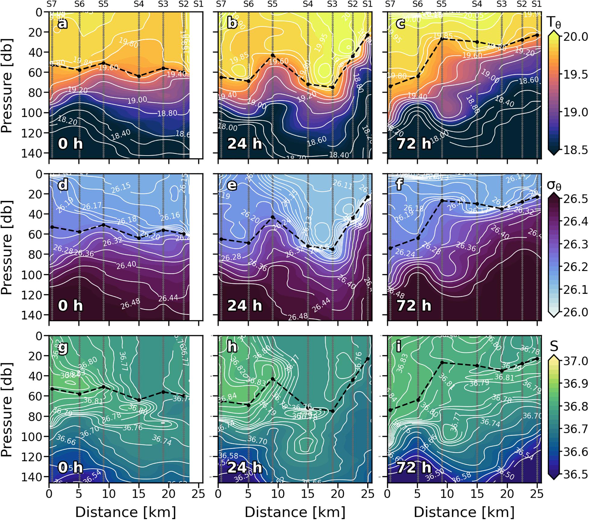
Figure 2. Vertical sections of potential temperature (T_q) (°C) (a–c), potential density (σ_q) (kg⋅m^–3) (d–f) and salinity (S) (g–i) for every sampling day. Stations are indicated in the upper part of the plot. Isopycnal field is superimposed as solid white lines. Dashed black line indicates the mixed layer depth. Sampling depths are represented by gray dots.

FIGURE 3

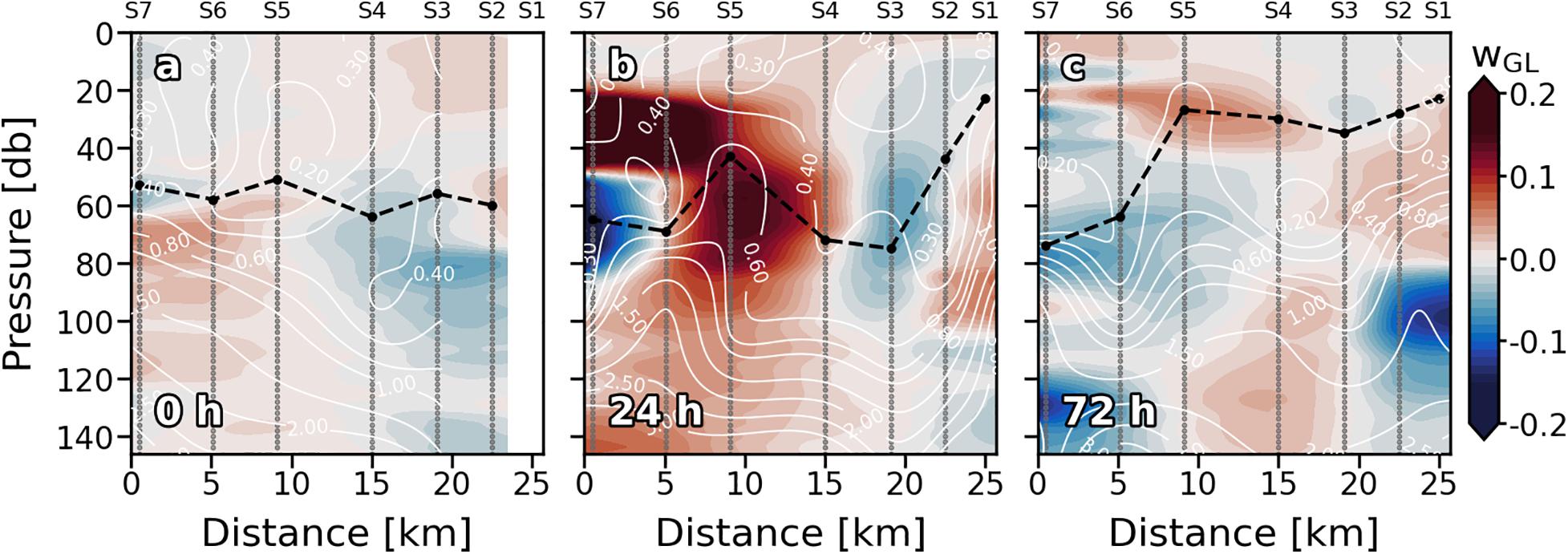
Figure 3. Vertical sections of vertical velocities (w_GL; m⋅day^–1) for every sampling days (a–c). Stations are indicated in the upper part of the plot. Nutrient (mmol⋅m^–3) field is superimposed as solid white lines. Sampling depths are represented by gray dots. Positive (negative) values indicate upward (downward) velocities. Dashed black line indicates the mixed layer depth.

Wind intensification in the first 24 h (Figures 1a,c) strengthened the front that led to a reinforcement of the 19.80°C isotherm, 26.15 kg⋅m^–3 isopycnal and 36.77 isohaline, deepening from ∼30 to ∼90 m and spreading from S5 and S6 to S3, S4, and S5 (Figures 2b,e,h). A doming of the isopleths associated with the front affected the entire S6. Like at 0 h, w_GL field was consistent with the physical structure. Vertical velocities also strengthened at 24 h (Figure 3b). Downward velocities were associated with the front-related downwelling whilst upward velocities coupled with isopleths upwelling. Thermocline (pycnocline) reshaped by the downwelling produced by the front, and the upwelling produced by the doming of the isopleths, presenting a vertical zig-zag pattern along the section.

On day 4 (72 h), neither wind intensity nor direction were favorable for front development (Figures 1b,c). Indeed, 19.80°C isotherm, 26.15 kg⋅m^–3 isopycnal and 36.77 isohaline horizontally crossed the whole section (Figures 2c,f,i). Nevertheless, a relative weak zig-zag pattern was still recognizable in the MLD similar to 24 h scenario (upwelling at S5 and S6, downwelling at S3 and S4; Figures 2b,e,h); probably a remnant of the thermocline deformation caused by the up- and downwelling fluxes driven by the front the day before. w_GL also maintained its bipolar structure between upwelling and downwelling stations above the MLD (Figure 3c). Below the isopleth doming observed at S5 and S6, counterpart bowl-shaped structure with negative w_GL highlights, both conforming a bipolar lentil-like shaped structure. Thermo and pycnocline were placed at ∼ 40 m at S1, S2, S3, and S4, whilst at ∼100 m at S6 and S7. The Shallowest thermo and pycnocline occurred at S5 associated with upwelling motions.

Though satellite-derived data should be used carefully in high-resolution cruises (as is the case) due to their significantly coarse horizontal resolution, a thermo-haline frontal zone is observed crossing through approximately the middle of the sampled section (Supplementary Figure 1) supporting our in situ observations. SST and SSS data also support the front temporal evolution of the front, showing a moderate intense front is observed at 0 and 24 h (Supplementary Figures 1A,B) compared with 72 h (Supplementary Figure 1D).

Biogeochemical Features

Nutrients (NO_x^–) present the typical vertical distributions of oligotrophic systems throughout the cruise (Figures 4a–c). Low values (<0.5 mmol⋅m^–3) were found at surface waters down to the thermocline, where NO_x^– increased into deeper waters (nitracline), reaching more than 3 mmol⋅m^–3 at 150 m. Nevertheless, this typical nutrient distribution is not consistent along the sections. At 0 h (Figure 4a), the nutricline did not coincide with the thermocline along the section, being deeper at S3 and S4 (∼120 m) compared with S5, S6, and S7 (∼80 m). Deeper nutricline at S3 and S4 coincides with downward w_GL below the MLD while shallower nutricline at S5, S6, and S7 is associated with upward velocities (Figure 3a). Highest NO_x^– values were found at S5, S6 and S7 below the MLD and at S3–S4 and S6–S7 above it. Notwithstanding, while high NO_x^– in the first stations seen to be linked to high NO_x^– concentrations below the MLD at S5–S6, high values at S6–S7 are not connected with NO_x^– maximums below the MLD. The most intense upward (positive) F_NOx below the MLD (Table 1) were observed at S5–S7 (0.039, 0.057, and 0.108 mmol⋅m^–2⋅d^–1, respectively) as well as the nutrient gradients (g_NOx). Negative values of g_NOx indicates a favorable nutrient gradients for upward fluxes. Comparing NO_x^– and F_NOx with the w_GL field, it could be observed that the higher values of NO_x^– and F_NOx at S5 and S6 were associated with most intense w_GL in the MLD as well as that w_GL in the MLD at S7 were negative (downward) which may be the reason of the detached high NO_x^– patch observed in the surface waters of S6–S7.

FIGURE 4

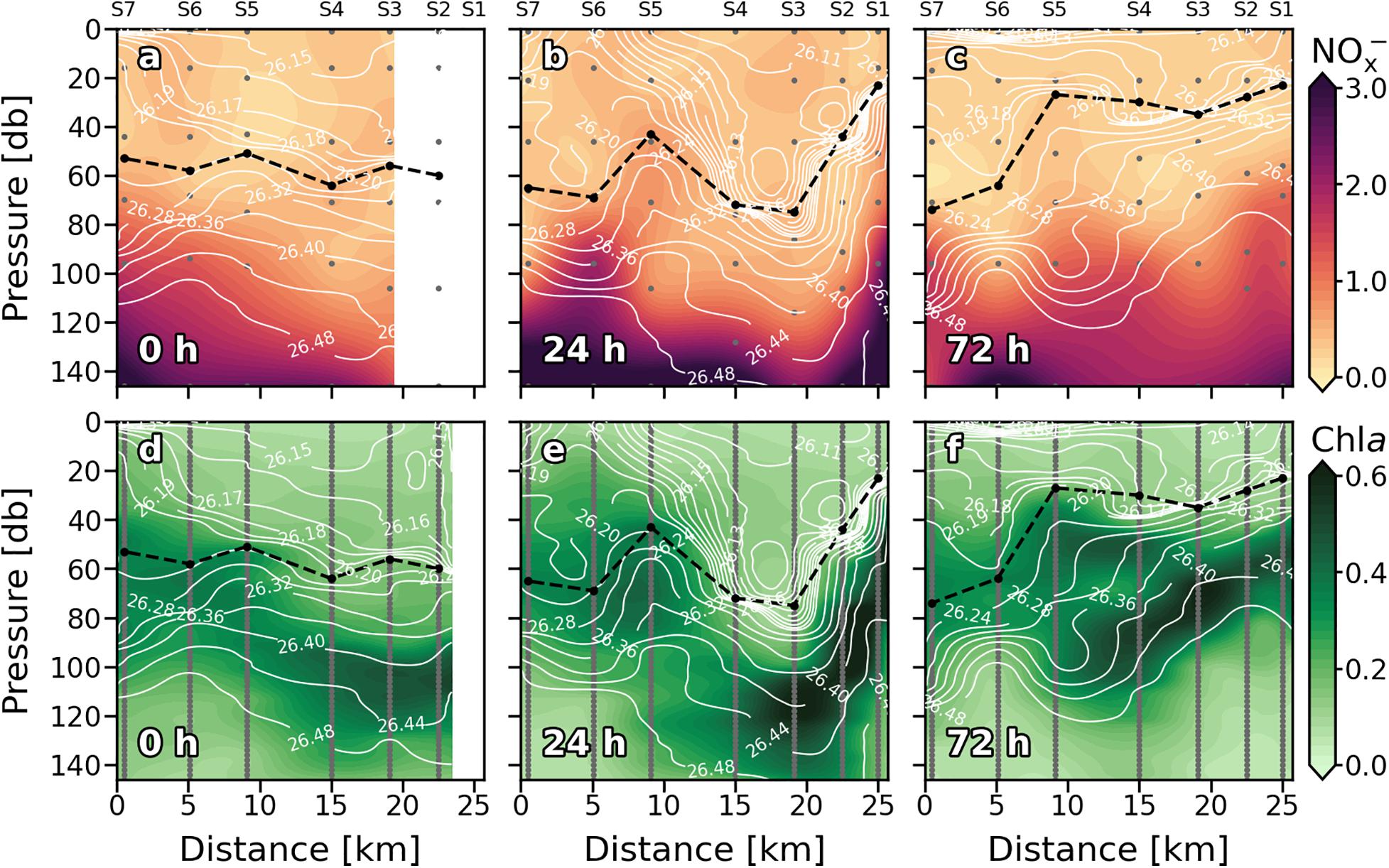
Figure 4. Vertical sections of nitrate + nitrite (NO_x^–) (mmol⋅m^–3) (a–c), and chlorophyll a (Chl a) (mg⋅m^–3) (d–f) for every sampling day. Stations are indicated in the upper part of the plot. Isopycnal field is superimposed as solid white lines. Dashed black line indicates the mixed layer depth. Sampling depths are represented by gray dots.

TABLE 1

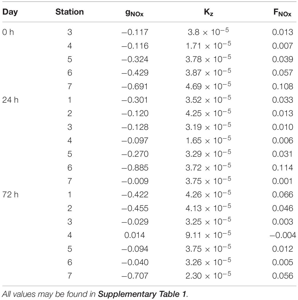
Table 1. Values of nutrient gradients (g_NOx; mmol⋅m^–3), vertical eddy diffusivity (K_z; m²⋅s^–1) and nutrient fluxes (F_NOx; mmol⋅m^–2⋅d^–1) right below the MLD.

The reshaping of the thermocline (pycnocline) by the reinforcement of the front at 24 h also reshaped the nutricline (Figure 4b), which shows the same zig-zag pattern observed in T_q and s_q Figure 2b). At S1 and S6, sloping of the isotherms introduced water with concentrations of about 2 mmol⋅m^–3 ∼ 40 m above the main thermocline reaching the surface at S6 while deepening of the isopleths at S2–S4 sinks surface waters to ∼ 90 m depth. The both, most intense positive and negative w_GL (Figure 3b) occurred associated with this isotherm sloping, respectively. The highest F_NOx and g_NOx were found at S6 and S1 (0.114 mmol⋅m^–2⋅d^–1) while lowest were found at S2–S4 and S7 (Table 1). In day four (72 h; Figure 4c), the doming of the isopleths below the MLD at S1–S2 and S7 introduced nutrient-richer waters from deeper layers into the bottom of the MLD (Figure 4b). Nevertheless, large amounts of NO_x^– inside the ML were observed at S1-S2 and S5 (Figure 4c). The highest F_NOx and g_NOx values right below to the MLD supports the upwelling of nutrients in those stations (Table 1), although w_GL did not completely agree with NO_x^– and F_NOx. Beside NO_x^– distribution suggest that a tongue of nutrient-richer waters outcrop from ∼100 m to about 20 m at S5, upward vertical velocities only dominated on the MLD while downward velocities are presented below the MLD.

Similarly, the vertical distribution of Chl a follows the characteristic pattern of an oligotrophic system (Figures 4d–f), presenting low values (<0.1 mg⋅m^–3) at surface waters, while a DCM was consistently observed over the nitracline. At 0 h (Figure 4d), the horizontal distribution of Chl a along the section revealed a discontinuity in the DCM between eastern stations (S1, S2, S3, and S4), where a deeper and more intense DCM occurred (0.4–0.5 mg⋅m^–3) and western stations (S5 and S6), as seen in nutricline (Figure 4a). This discontinuity became obvious when the front intensified at 24 h (Figure 4e). An intense DCM (∼0.6 mg⋅m^–3) due to the front-driven sloping of the isotherms was placed at 40 m at S1 and at ∼150 m at S3 and S4. Relatively high values of Chl a were also observed at 24 h in surface waters of S6 and S7, coinciding with nutrient upwelling (Figure 4b). In the western stations, the DCM remained centered at 60 m depth. However, a slightly increase in Chl a (∼0.45 mg⋅m^–3) coincided with nutrient upwelling in S5. Weakening of the front at 72 h (Figure 4f) resulted in an overlap of the two DCM cores at S5 coinciding with the lentil-like shaped structure described in the section above (Figures 2c,d).

Picoplankton Distribution and Community Structure

Maximum values of Prochlorococcus (Pro) biomass were generally distributed between subsurface waters (>20 m) and just above the DCM throughout the cruise (Figures 5a–c). At 0 h (Figure 5a), Pro biomass was widely distributed along the section presenting higher values in the MLD of S3, S4, and S5. On the second sampling day (Figure 5b), Pro biomass decreased, and the maximum values were associated with upwelling velocities at S4, S5, and S6 (Figure 3b). At 72 h (Figure 5c), the highest Pro biomass values were found at S2 at 60 m coinciding with positive (upward) w_GL and F_NOx (Figure 3c and Table 1). The highest Pro biomass values were consistently placed in nutrient upwelling zones.

FIGURE 5

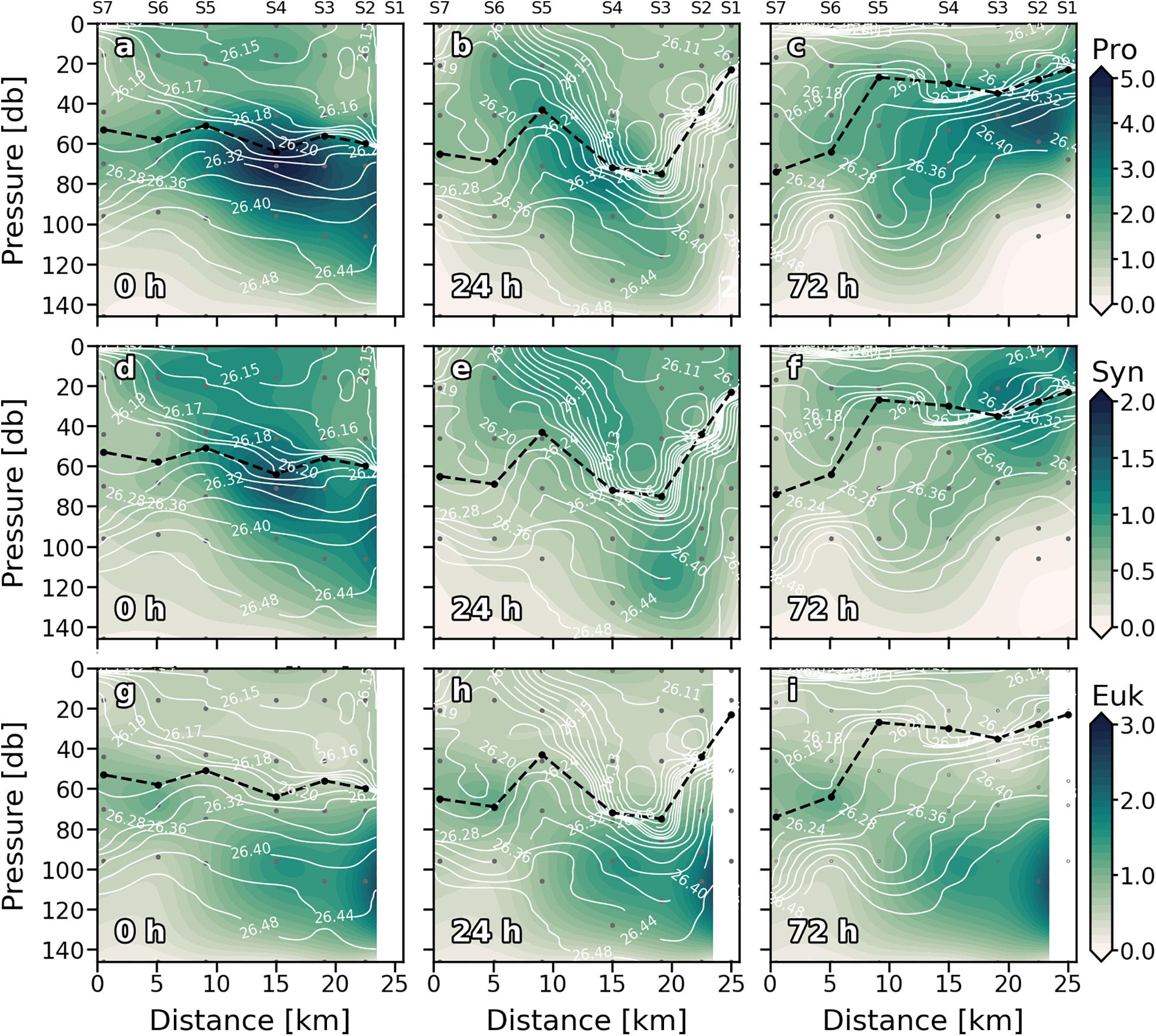
Figure 5. Vertical sections of phytoplankton biomass (mg C⋅m^–3) of Prochlorococcus sp. (Pro) (a–c); Synechococcus sp. (Syn) (d–f) and Eukaryotes (Euk) (g–i) for every sampling day. Stations are indicated in the upper part of the plot. Isopycnal field is superimposed as solid white lines. Dashed black line indicates the mixed layer depth. Sampling depths are represented by gray dots.

Synechococcus (Syn) was generally widely distributed in the well-mixed waters above the thermocline (Figures 5d–f). Like Pro, Syn presented its highest biomass at S4 in the first sampling day (Figure 5d). At 24 h (Figure 5e) the general Syn biomass distribution changed, and high Syn biomass values were found below the thermocline, at the base of the front (∼120 m). Deep high Syn biomass values were also observed on day four (72 h; Figure 5f) associated with the downwelling occurred below the MLD at S5. Nevertheless, maximum values at 72 h were found in surface waters of S1 and S2. The distribution of the Euk and the DCM resembled throughout the first 24 h (Figures 5g,h). At 72 h the relationship between Euk and DCM distribution was observed along S4–S7, while maximum values of Euk biomass were found below the DCM (MLD) in S1–S3 breaking with the observed general pattern (Figure 5i).

Water column integrated biomass values are compiled in Table 2. At 0 h, all picoplankton groups present higher integrated biomass in the eastern stations, showing Cyanobacteria group differences of up to 3-fold between both ends of the section (S2 and S7). Differences of up to 2-fold between S4 and S6 separated by ∼10 km in Cyanobacteria’s biomass can be observed. Pro is the major contributor to picoplankton community biomass along the section at 0 h (56.59 ± 2.64%), while Syn and Euk show similar contributions to total biomass (22.68 ± 3.88% and 20.73 ± 1.43%, respectively; Figure 6a). With the enhancement of the front on day two (24 h) the highest Cyanobacteria biomasses are observed at the front-associated stations (S3–S5) while both ends of the section show similar values (Table 2). Nevertheless, differences are not as high as at 0 h. Euk presents a consistent integrated biomass along the section at 24 h. Pro still is the major contributor to the total biomass (51.32 ± 7.88%) except in S2 where Euk and Pro show similar contribution rates (38.81% and 38.04%, respectively; Figure 6b). At 72 h, both Syn and Euk present similar integrated values among the stations. Pro keeps showing higher values in front-affected stations (S2–S5) as well as in the major contribution percentages to total biomass (48.16 ± 2.51%; Figure 6c).

TABLE 2

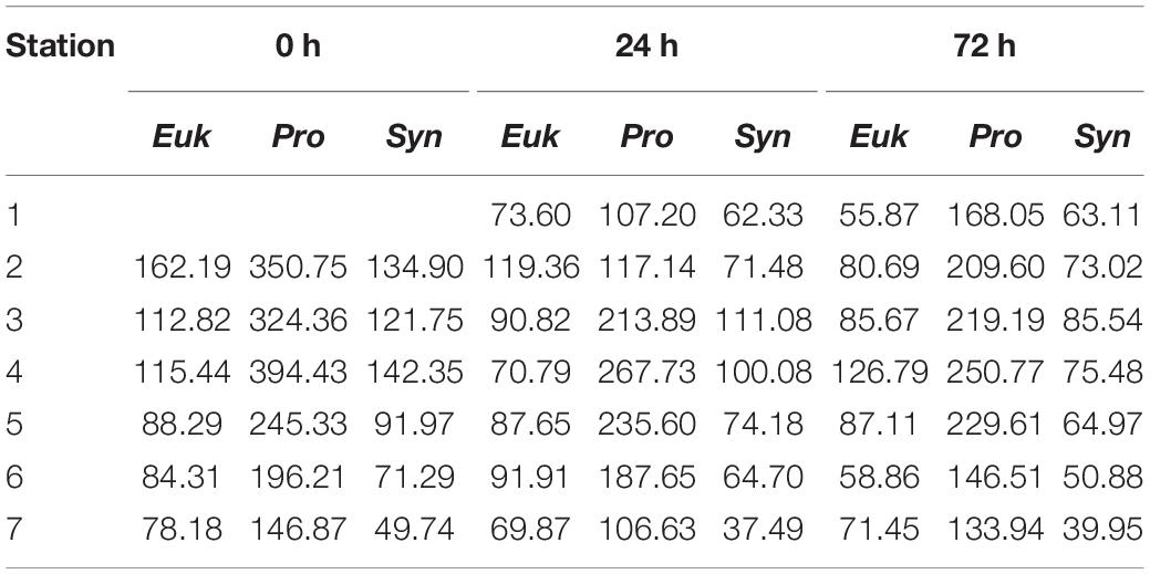
Table 2. Integrated biomass (mg C⋅m−²) between surface and 150 m depth of Eukaryotes (Euk), Prochlorococcus sp. (Pro) and Synechococcus sp. (Syn) for the three sampling days (0, 24, and 48 h) and for every station.

FIGURE 6

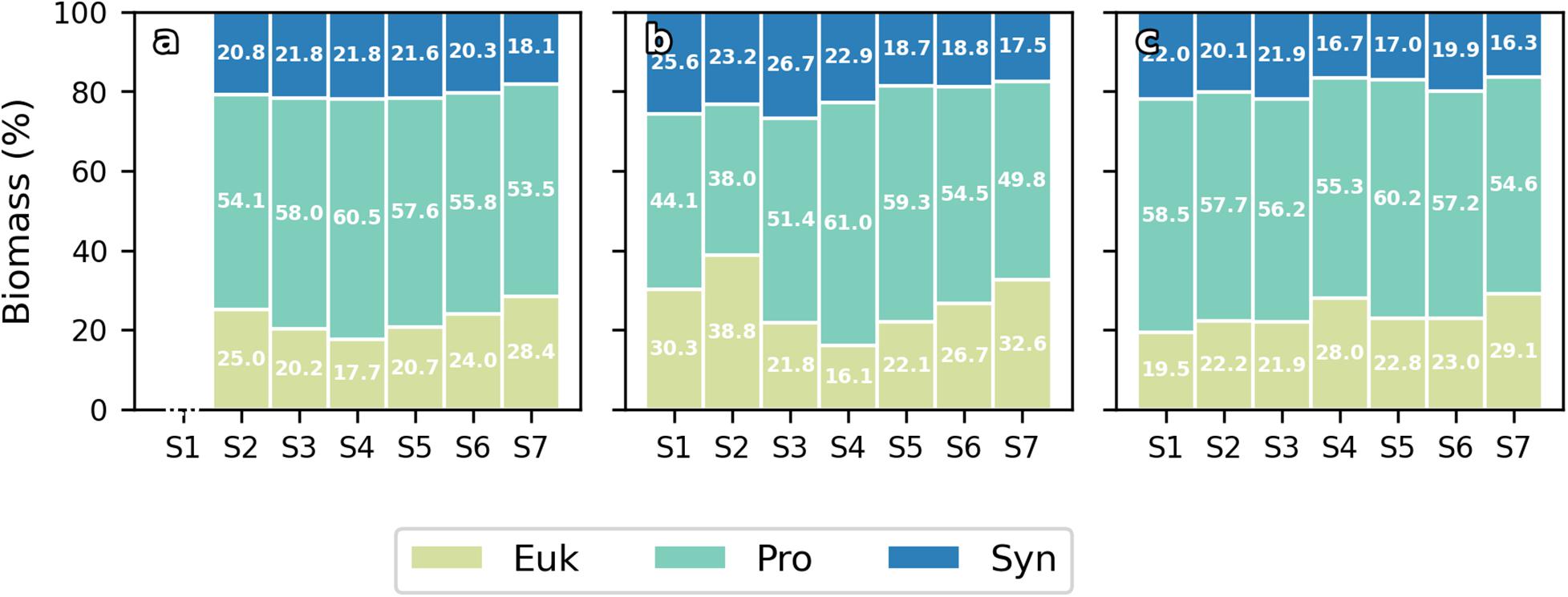
Figure 6. Bar plots of contribution (%) of Eukaryotes (Euk), Prochlorococcus sp. (Pro) and Synechococcus sp. (Syn) to total integrated biomass at 0 h (a), 24 h (b), and 72 h (c) for every station.

Front Effects Over the Community Structure

Metric Multidimensional Scaling Analysis sorts stations according to differences in picoplankton community structure. Therefore, closer stations present similar picoplankton community assemblages and vice versa. At 0 h, three stations groups were obtained from K-means clustering method (Figure 7A): (1) S2, S3, and S4 where front-driven up motions occurred; (2) S5 and S6, that were situated at the western boundary of the front; and (3) S7, the farthest from the front. At 24 h (Figure 7B), three groups were also observed: (1) S1, S2, and S7, that represent the eastern and western boundaries of the front; (2) S3, S4, and S5 situated at the upwelling front; and (3) S6, where the upwelling front occurs. The vanishing of the front at 72 h also lead to the vanishing of community structure heterogeneity and no significant differences were observed among station in community structure (Figure 7C). The selection of three groups at 0 h and 24 h was supported by high BSS/TSS ratio (91.7% and 85.1%, respectively). At 72 h the BSS/TSS ratio is not displayed since there were no differences among stations.

FIGURE 7

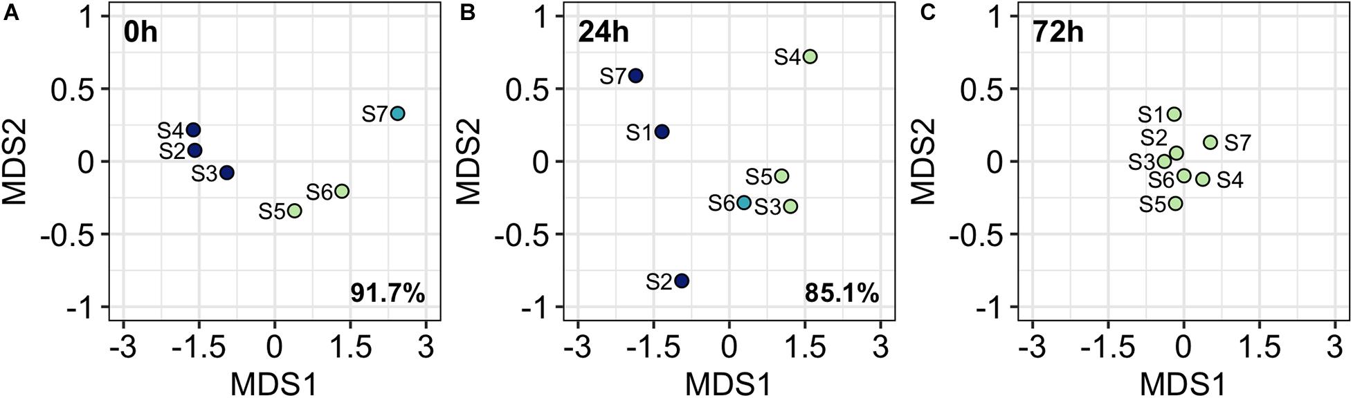
Figure 7. Metric Dimensional Scaling analysis (MDS) ordination plots at 0 h (A), 24 h (B), and 72 h (C). Colors refer to K-mean clustering results. Percentage refers to the BSS/TSS ratio. No BSS/TSS ratio is reported at 72 h since stations are grouped in only one cluster.

Spatial vs. Temporal Variability

The contributions of every source of variability to total variance are compiled in Table 3. Depending on the phytoplankton group, two behaviors may be observed in the entire water column. Cyanobacteria-like Pro and Syn present higher space variability (i.e., among station in the same day), while Euk presents higher temporal variability. This pattern is not observed in the DCM, where all phytoplankton groups show higher temporal than spatial variability. Inside the mixed layer, phytoplankton groups present almost equally spatiotemporal variability. Chl a shows higher temporal variability in all cases.

TABLE 3

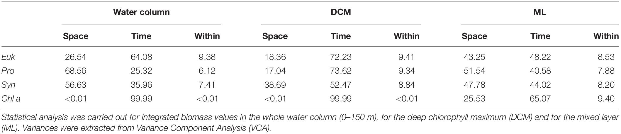
Table 3. Percentage of total variance for each source of variability: Distance among stations (Space), daily variability (Time), and the inner variability (Within) for Eukaryotes (Euk), Prochlorococcus sp. (Pro), Synechococcus sp. (Syn), and Chlorophyll a (Chl a).

Discussion

Wind Forcing Frontogenesis

Oceanic fronts originated south of Gran Canaria in the area of eddy formation at the wind shear flanks were reported in earlier studies describing the eddy field in the region (Arístegui et al., 1994, 1997; Barton et al., 1998). Later, Barton et al. (2000) and Basterretxea et al. (2002), in more front-focused studies, suggested a potential mechanism for their development. They observed that wind velocities dropped down up to one order of magnitude at the lee region of the island with respect to a station placed in the wind exposed region ∼2 km apart. As a consequence, net westward Ekman transport in the lee region would be practically absent, favoring the convergence (divergence) of water in the eastern (western) side of the wake and its subsequent downwelling (upwelling).

The data presented here fit the Barton et al. (2000) and Basterretxea et al. (2002)’s spatial wind field observations (Figures 1a,b) but they also indicate a positive temporal relationship between wind speed and front intensity. During the first 48 h, the increase in down-front blowing winds (Figure 1c) strengthened the front signal as seen in T_q, s_q, and S plots (Figures 2a,b,d,e,g,h). Conversely, the change in wind direction at 72 h (up-front winds) caused the vanishing of the front signal and the increase in water column stratification, as suggested by the shallowest MLD (Figures 2c,f,i). This agrees with the nonlinear Ekman effect theory for frontogenesis of Thomas and Lee (2005), that proposes that winds blowing in the direction of the geostrophic flow generate an Ekman flux that tends to advect colder water from one side of the front over warmer water from the other side, enhancing convective mixing and, thus, strengthening the front. ASC-related upwelling in the warm side of the front and downwelling in the cold side would be triggered as consequence of convective mixing (Nagai et al., 2006; Pallàs-Sanz et al., 2010). By contrast, winds blowing against geostrophic flow generate the advection of warmer water over colder water favoring vertical stratification and, hence, the weakening of the front (frontolisis). This theory has been later sustained by several modeling and numerical studies (Thomas, 2005; Thomas and Lee, 2005; Thomas and Ferrari, 2008; Mahadevan et al., 2010).

The bipolar structure (upwelling/downwelling; warm/cold) described by the nonlinear Ekman effect theory agrees with the physical structure clearly shown in Figures 2b, 3b. A steep deepening of the isotherm in S2–S4 sinks water in the cold side of the front while doming of the isotherm in S5 and S6 entrained deep waters in the warm side suggesting downwelling and upwelling motions, respectively. This is supported by downward and upward w_GL coinciding with S2–S4 and S5 and S6. At 0 h, only the upwelling side of the front is observed (Figures 2a, 3a), being characterized by a less intense doming of the isotherm in the warm side (S2–S4) compared to the one observed at 24 h. Notwithstanding, positive w_GL were also observed at these stations, coinciding with 24 h observations.

Effects of Frontal Dynamics Over Nutrient Distribution

Subtropical oligotrophic areas such as the Canary region are characterized by a well sun light illuminated mixed layer throughout the year, with very low inorganic nutrient concentrations (Levitus et al., 1993) due to the presence of a strong almost permanent thermocline that prevents the outcrop of deeper nutrient-rich waters into the euphotic zone (León and Braun, 1973). It has been suggested that ASC associated with submesoscale fronts may locally alleviate nutrient shortage in oligotrophic surface waters by driving vertical nutrient fluxes into the ML (Mahadevan and Tandon, 2006; Lévy et al., 2012a; Estrada-Allis et al., 2019).

In the present case, the canonical oligotrophic nutrient distribution was broken by high nutrient concentrations that outcropped trough the thermocline into the ML in S4 and S3 at 0 h; S6 at 24 h, and S5 at 72 h (Figures 4a–c). In all cases, nutrient intrusions were associated with isopleths doming driven by front-associated upwelling, where positive (upward) w_GL and F_NOx near the MLD occurred. Though small, the upward fluxes are consistent with other observations in areas of intense mesoscale and submesoscale activity (Arcos-Pulido et al., 2014; Corredor-Acosta et al., 2020). The overlapping of positive w_GL with F_NOx suggests that diapycnal mixing is acting as an important contributor to the vertical velocity (Ponte et al., 2013) and may be associated with submesoscale process (Estrada-Allis et al., 2019). In summary, upward movements at each side of the front favors the injection of NO_x into the euphotic layer as well as downward motions deepens the nutricline impoverishing the ML, supporting earlier theoretical studies (Lévy et al., 2018 and reference therein).

Does Frontal Dynamics Modulate Picoplankton Distribution and Community Structure?

The picoplankton distribution presented here (see Figure 5) largely corroborates the commonly reported distribution described for each group in the region (e.g., Baltar et al., 2009). Syn was abundant in the well-mixed surface layers (Mackey et al., 2013; Grébert et al., 2018), whereas higher amounts of Pro were present in deeper layers (Bouman et al., 2006; Johnson et al., 2006; Biller et al., 2015). Euk were the main contributors to DCM laying close to the nitracline, suggesting that they require higher inorganic nutrients concentrations than prokaryotic phytoplankton for their growth (Painter et al., 2014). Nonetheless, these general distributions were eventually modified by frontal dynamics.

For instance, we observed high Syn concentrations at ∼150 m depth at 24 h coinciding with the downwelling branch of the front. This distribution agrees with the subduction of phytoplankton by submesoscale front-associated downwelling as proposed by several authors (Lévy et al., 2001, 2012a, 2018). Whether the front-driven enlargement of the mixed layer at this station was responsible for the Syn distribution observed or, by contrast, Syn cells found at these depths were dragged from surface waters due to front intensification, is difficult to discern, although front dynamics seem to be behind the distribution patterns in both cases. High Euk biomass at 72 h found below the DCM and the MLD of S1, S2, and S3, is another example of how frontal dynamics subducts phytoplankton biomass. In this case, the high Euk biomass patch appears to be a leftover from the intense DCM observed at 24 h, which has been left out the ML due to frontolisis restratification.

One of the most striking exceptions to the usually reported picoplankton distribution is observed in Pro. The fact that high Pro biomass patches consistently coincided with high nutrient concentrations (Figures 3a–c, 4a–c) differs from the distribution patterns previously reported in the literature. Due to their high nutrient diffusion per unit of cell volume (Raven, 1998; Marañón, 2015) and their capacity of uptake dissolved organic matter (DOC) for growth (Berman and Bronk, 2003; Mulholland and Lee, 2009; Znachor and Nedoma, 2010; Duhamel et al., 2018; osmotrophy), Pro inorganic nutrient requirements are low and thus, they usually present higher abundances in nutrient-poor zones (Bouman et al., 2006; Johnson et al., 2006; Biller et al., 2015). Indeed, several studies have reported low Pro abundances related to eddy-driven nutrient upwelling in the region along with high Pro biomass associated with high dissolved organic matter concentrations (Baltar et al., 2009; Hernández-Hernández et al., 2020). Maximum DOC concentrations along the cruise (not shown here) also coincided with Pro biomass peaks. For these reasons, we considered that Pro and NO_x^– maximums resemblance seems to be a coincidence rather than a causality, and that front-driven accumulation of DOC would be the reason of high abundances of Pro at nutrient upwelling stations.

Besides the general distribution, the data presented in Figure 5 reveal high biomass patches for every picoplankton group. Several authors have reported local increases of different phytoplankton size groups across frontal zones due to the input of nutrients in a constrained zone, which usually favors the growth of large cells such as diatoms (Abraham, 1998; Rivière and Pondaven, 2006; Mahadevan et al., 2012). D’Ovidio et al. (2010) observed that phytoplankton is organized in submesoscale patches of dominant types separated by physical barriers. Our data reflect two main differences with respect to the studies mentioned above: (1) previous works observed that patches were dominated by different phytoplankton size-groups (i.e., pico, nano, or microplankton; Abraham, 1998; Rivière and Pondaven, 2006; D’Ovidio et al., 2010; Mahadevan et al., 2012), while we observed that patchiness also occurs within the same size-group. This finding raises the question of at what level of organization patchiness actually works. (2) They observed high biomass patches related with local nutrient injection (Abraham, 1998; Rivière and Pondaven, 2006; D’Ovidio et al., 2010; Mahadevan et al., 2012). In our study, by contrast, only Pro high abundance spots are related to high nutrient concentrations albeit this is probably not due to a causality, as we explained above. While it is true that we only report picoplankton data, the occurrence of these non-nutrient related “hotspots” of high picoplankton biomass suggests that submesoscale dynamics modulates both the hydrographic and biogeochemical fields, favoring the local growth of some groups against others. It is known that although picoplankton groups generally co-occur in subtropical oceans, they present different nutrient requirements, light harvesting, different temperature or physical forcing acclimation (Moore et al., 2002; Scanlan et al., 2009; Mella-Flores et al., 2012; Flombaum et al., 2013; Otero-Ferrer et al., 2018). Therefore, picoplankton groups’ distribution across a submesoscale front would be expected to be affected by the front-generated physical and biogeochemical variability (Lévy et al., 2018 and references therein).

A relevant result of our study is the modulation of the picoplankton community structure by the front. Phytoplankton community assemblages were strongly structured in the MDS ordination space in accordance with the frontal structure (Figure 7). Few studies have reported the variability in phytoplankton community structures across a frontal systems at submesoscale level (e.g., Taylor et al., 2012; Clayton et al., 2014; Mousing et al., 2016). In all of these studies, different assemblages were observed; at each side of the front and within the front, as the result of the separation of two well-defined water masses and hence two different biomes, with two different communities. Conversely, we observed that picoplankton communities were not separated by the front but showed a mirror-like distribution with respect to the middle of the front. While observations from previously cited authors suggest that fronts work like a physical barrier for different niches, our results suggest that frontal dynamics modulates the phytoplankton community structure. However, it should be noted that while fronts reported by the authors mentioned above were permanent features that separate different water masses, we sampled an ephemeral front that is originated inside the same water mass (Lévy et al., 2018).

Due to section proximity to the coast, tidal forcing was initially considered as another potential driver for the observed picophytoplankton variability. Sangrá et al. (2001) studied the effect of internal waves on Chl a in the shelf break of the lee region of Gran Canaria during a spring and a neap tide. They reported an increase in Chl a of up to 47% during some pulses of the spring tide from a station situated over the shelf (100 m depth). Notwithstanding, depth integrated Chl a values presented little differences between samplings. Since our section was situated on the 2,000 m isobath (i.e., the island slope), the cruise took place during a full neap tide, and phytoplankton biomass increases were significantly larger than those reported by Sangrá et al. (2001), we considered that the tidal forcing effects if any, they would be negligible compare to front-related effects.

Spatiotemporal Variability

In an earlier study, Martin et al. (2005) observed higher variability in picoplankton community biomass at mesoscale ranges than in the normally used large-scale ranges, arguing that sampling should be done at smaller scales to avoid inaccurate plankton distributions. The integrated biomass data presented here (Table 2) reveal that picoplankton biomass varies between 2 and 3-fold on spatial scales of ∼ 2.5 km, and temporal scales of ∼ 24 h. This variability is comparable to the picoplankton biomass seasonality reported for the region (Zubkov et al., 2000b; Baltar et al., 2009).

In order to assess which source of variability was dominant, we compared the temporal and spatial variances observed during our study (Table 2). We found that picoplankton biomass variance is almost equally shared between time and space in the mixed layer, while it mostly depends on time in the DCM, i.e., in the front reported here, picoplankton biomass temporal variability is just as important as, or even more important than spatial variability. Although the front is constrained to a marginal part of the Canary Current region, mesoscale processes and associated submesoscale motions, are ubiquitous around the global ocean (Chelton et al., 2007, 2011). Therefore, our results beg to question whether oceanographic samplings in regions of high mesoscale activity should be designed considering submesoscale spatiotemporal resolutions, in order to gain a more accurate approximation of the biogeochemical fields variability in the region of study.

Conclusion

The spatiotemporal development and decay of the convergent wind-driven submesoscale front south of Gran Canaria, as well as their effects on picoplankton community structure and distribution, is reported for the first time through in situ measurements. Like in earlier studies in the region (Barton et al., 2000; Basterretxea et al., 2002), our data shows a positive relationship between wind and front development and intensity. Upward diapycnal nutrient flux occurs near the mixed layer of the stations located on the front. This diapycnal mixing was implicated in the observed enhancement of nutrients and chlorophyll in the upper layer advected by positive vertical velocities based on the scaling of Garret and Loder (1981). Conversely, picophytoplankton biomass subduction is also reported. The present study is consistent with model outputs and past predictions, supporting that submesoscale fronts may drive nutrient fluxes into the euphotic layer and subduct picoplankton biomass below it (Mahadevan and Archer, 2000; Lévy et al., 2001, 2012a).

On the other hand, our results also provide new insights in front formation and erosion, pointing out to nonlinear Ekman effects as a potential driver of front dynamics, and their effects on picoplankton community structure. The front favors the patch formation of different picoplankton groups’ dominance and modulates the picoplankton community structure. Temporal variability was found to be a significant source of error in phytoplankton variability providing evidence that, at least in regions of high hydrographic variability, plankton, as well as other biogeochemical features, must be sampled at shorter spatial and temporal resolutions than regularly done in order to obtain more accurate datasets. Although daily repeated cruises are in many cases economically unviable and time-consuming, submesoscale measurements would help to get more accurate regional and long-term interpretation of biogeochemical fluxes.

It is worth mentioning that the physical results presented in this study are constrained by the spatiotemporal scales of the survey and the lack of horizontal velocities. However, validated parameterizations and solid scaling of the vertical velocity formulations, allow us to provide a first approximation of submesoscale and diapycnal mixing impact on the biological system in the leeward side of Gran Canaria Island.

Data Availability Statement

The data sets generated for this study are available on request to the corresponding author.

Author Contributions

JA conceived and designed the cruise. NH-H, YS-F, and JA carried out the sampling and data analyses. SE-A contributed to the analysis of the physical data. NH-H wrote the manuscript with inputs from all authors. All authors contributed to the article and approved the submitted version.

Funding

This work is a contribution to the projects PUMP (CTM2012-33355), FLUXES (CTM2015-69392-C3-1-R), and e-IMPACT (PID2019-109084RB-C2) from the Spanish “Plan Nacional de I+D,” co-funded with FEDER funds, and project TRIATLAS (AMD-817578-5) from the European Union’s Horizon 2020 Research and Innovation Program. NH-H was supported by a grant (TESIS2015010036) of the Agencia Canaria de Investigación, Innovación y Sociedad de la Información (ACIISI).

Conflict of Interest

The authors declare that the research was conducted in the absence of any commercial or financial relationships that could be construed as a potential conflict of interest.

Acknowledgments

We thank to the members of the Biological Oceanography group (GOB-IOCAG) for their help with the analysis of the samples, and Laura Marín for reviewing the English grammar.

Supplementary Material

The Supplementary Material for this article can be found online at: https://www.frontiersin.org/articles/10.3389/fmars.2021.592703/full#supplementary-material

Supplementary Figure 1 | Sea surface temperature (°C) time series for (A) May 09th 2011 (0 h), (B) May 10th 2011 (24 h), (C) May 11th 2011 (48 h), and (D) May 12th 2011 (72 h). Salinity contours are superimposed to SST maps. Black dots with red borders indicate stations positions. Red dot indicates Gando airport location.

Supplementary Figure 2 | Vertical sections of Turner angles (T_U; °) for 0 h (A), 24 h (B), and 72 h (C). Stations are indicated in the upper part of the plot. Dashed black line indicates the mixed layer depth. Sampling depths are represented by gray dots. Angles between −90 and −45 are characteristic of diffusive mode; between −45° and 45° is called doubly stable mode; weak salt fingers mode from 45° to 70° and salt finger mode for angles larger than 70.

Supplementary Table 1 | Values of nutrient gradients (g_NOx; mmol⋅m^–4), vertical eddy diffusivity (K_z; m²⋅s^–1), nutrient fluxes (F_NOx; mmol⋅m^–2⋅d^–1) below the MLD for all sampled depths.

Footnotes

1. ^ http://www.r- project.org

References

Abraham, E. R. (1998). The generation of plankton patchiness by turbulent stirring. Nature 391, 577–581. doi: 10.1038/35361

CrossRef Full Text | Google Scholar

Allen, J. T., Brown, L., Sanders, R., Moore, C. M., Mustard, A., Fielding, S., et al. (2005). Diatom carbon export enhanced by silicate upwelling in the northeast Atlantic. Nature 437, 728–732. doi: 10.1038/nature03948

PubMed Abstract | CrossRef Full Text | Google Scholar

Arcos-Pulido, M., Rodríguez-Santana, A., Emelianov, M., Paka, V., Arístegui, J., Benavides, M., et al. (2014). Diapycnal nutrient fluxes on the northern boundary of Cape Ghir upwelling region. Deep. Res. Part I Oceanogr. Res. Pap. 84, 100–109. doi: 10.1016/j.dsr.2013.10.010

CrossRef Full Text | Google Scholar

Arístegui, J., Barton, E. D., Álvarez-Salgado, X. A., Santos, A. M. P., Figueiras, F. G., Kifani, S., et al. (2009). Sub-regional ecosystem variability in the Canary Current upwelling. Prog. Oceanogr. 83, 33–48. doi: 10.1016/j.pocean.2009.07.031

CrossRef Full Text | Google Scholar

Arístegui, J., Sangrá, P., Hernández-León, S., Cantón, M., Hernández-Guerra, A., and Kerling, J. L. (1994). Island-induced eddies in the Canary islands. Deep. Res. Part I 41, 1509–1525. doi: 10.1016/0967-0637(94)90058-2

CrossRef Full Text | Google Scholar

Arístegui, J., Tett, P., Hernández-Guerra, A., Basterretxea, G., Montero, M. F., Wild, K., et al. (1997). The influence of island-generated eddies on chlorophyll distribution: a study of mesoscale variation around Gran Canaria. Deep. Res. Part I Oceanogr. Res. Pap. 44, 71–96. doi: 10.1016/S0967-0637(96)00093-3

CrossRef Full Text | Google Scholar

Baltar, F., Arístegui, J., Montero, M. F., Espino, M., Gasol, J. M., and Herndl, G. J. (2009). Mesoscale variability modulates seasonal changes in the trophic structure of nano- and picoplankton communities across the NW Africa-Canary Islands transition zone. Prog. Oceanogr. 83, 180–188. doi: 10.1016/j.pocean.2009.07.016

CrossRef Full Text | Google Scholar

Barton, E. D., Aristegui, J., Tett, P., Canton, M., García-Braun, J., Hernández-León, S., et al. (1998). The transition zone of the Canary Current upwelling region. Prog. Oceanogr. 41, 455–504. doi: 10.1016/S0079-6611(98)00023-8

CrossRef Full Text | Google Scholar

Barton, E. D., Basterretxea, G., Flament, P., Mitchelson-jacob, E. G., Jones, B., Arístegui, J., et al. (2000). Lee region of Gran Canaria. J. Geophys. Res. 105, 173–193.

Google Scholar

Basterretxea, G., Barton, E. D., Tett, P., Sangrá, P., Navarro-Perez, E., and Arístegui, J. (2002). Eddy and deep chlorophyl maximum response to wind-shear in the lee of Gran Canaria. Deep. Res. Part I Oceanogr. Res. Pap. 49, 1087–1101. doi: 10.1016/S0967-0637(02)00009-2

CrossRef Full Text | Google Scholar

Berman, T., and Bronk, D. A. (2003). Dissolved organic nitrogen: a dynamic participant in aquatic ecosystems. Aquat. Microb. Ecol. 31, 279–305. doi: 10.3354/ame031279

CrossRef Full Text | Google Scholar

Biller, S. J., Berube, P. M., Lindell, D., and Chisholm, S. W. (2015). Prochlorococcus: the structure and function of collective diversity. Nat. Rev. Microbiol. 13, 13–27. doi: 10.1038/nrmicro3378

PubMed Abstract | CrossRef Full Text | Google Scholar

Bouman, H. A., Ulloa, O., Scanlan, D. J., Zwirglmaier, K., Li, W. K. W., Platt, T., et al. (2006). Oceanographic basis of the global surface distribution of Prochlorococcus ecotypes. Science 312, 918–921. doi: 10.1126/science.1122692

PubMed Abstract | CrossRef Full Text | Google Scholar

Capet, X., McWilliams, J. C., Molemaker, M. J., and Shchepetkin, A. F. (2008). Mesoscale to submesoscale transition in the California Current system. Part II: frontal processes. J. Phys. Oceanogr. 38, 44–64. doi: 10.1175/2007JPO3672.1

CrossRef Full Text | Google Scholar

Chelton, D. B., Schlax, M. G., and Samelson, R. M. (2011). Global observations of nonlinear mesoscale eddies. Prog. Oceanogr. 91, 167–216. doi: 10.1016/j.pocean.2011.01.002

CrossRef Full Text | Google Scholar

Chelton, D. B., Schlax, M. G., Samelson, R. M., and de Szoeke, R. A. (2007). Global observations of large oceanic eddies. Geophys. Res. Lett. 34, 1–5. doi: 10.1029/2007GL030812

CrossRef Full Text | Google Scholar

Clayton, S., Nagai, T., and Follows, M. J. (2014). Fine scale phytoplankton community structure across the Kuroshio Front. J. Plankton Res. 36, 1017–1030. doi: 10.1093/plankt/fbu020

PubMed Abstract | CrossRef Full Text | Google Scholar

Corredor-Acosta, A., Morales, C. E., Rodríguez-Santana, A., Anabalón, V., Valencia, L. P., and Hormazabal, S. (2020). The influence of diapycnal nutrient fluxes on phytoplankton size distribution in an area of intense mesoscale and submesoscale activity off Concepción, Chile. J. Geophys. Res. Ocean 125:e2019JC015539. doi: 10.1029/2019JC015539

CrossRef Full Text | Google Scholar

Cotti-Rausch, B. E., Lomas, M. W., Lachenmyer, E. M., Goldman, E. A., Bell, D. W., Goldberg, S. R., et al. (2016). Mesoscale and sub-mesoscale variability in phytoplankton community composition in the Sargasso Sea. Deep. Res. Part I Oceanogr. Res. Pap. 110, 106–122. doi: 10.1016/j.dsr.2015.11.008

CrossRef Full Text | Google Scholar

D’Asaro, E., Lee, C., Rainville, L., Harcourt, R., and Thomas, L. (2011). Enhanced turbulence and energy dissipation at ocean fronts. Science 332, 318–322. doi: 10.1126/science.1201515

PubMed Abstract | CrossRef Full Text | Google Scholar

de Boyer Montégut, C., Madec, G., Fischer, A. S., Lazar, A., and Iudicone, D. (2004). Mixed layer depth over the global ocean: an examination of profile data and a profile-based climatology. J. Geophys. Res. C Ocean. 109, 1–20. doi: 10.1029/2004JC002378

CrossRef Full Text | Google Scholar

D’Ovidio, F., De Monte, S., Alvain, S., Dandonneau, Y., and Lévy, M. (2010). Fluid dynamical niches of phytoplankton types. Proc. Natl. Acad. Sci. U.S.A. 107, 18366–18370. doi: 10.1073/pnas.1004620107

PubMed Abstract | CrossRef Full Text | Google Scholar

Duhamel, S., Van Wambeke, F., Lefevre, D., Benavides, M., and Bonnet, S. (2018). Mixotrophic metabolism by natural communities of unicellular cyanobacteria in the western tropical South Pacific Ocean. Environ. Microbiol. 20, 2743–2756. doi: 10.1111/1462-2920.14111

PubMed Abstract | CrossRef Full Text | Google Scholar

Estrada-Allis, S. N., Barceló-Llull, B., Pallàs-Sanz, E., Rodríguez-Santana, A., Souza, J. M. A. C., Mason, E., et al. (2019). Vertical velocity dynamics and mixing in an anticyclone near the Canary Islands. J. Phys. Oceanogr. 49, 431–451. doi: 10.1175/JPO-D-17-0156.1

CrossRef Full Text | Google Scholar

Falkowski, P. G., Ziemann, D., Kolber, Z., and Bienfang, P. K. (1991). Role of eddy pumping in enhancing primary production in the ocean. Nature 352, 55–58. doi: 10.1038/352055a0

CrossRef Full Text | Google Scholar

Flombaum, P., Gallegos, J. L., Gordillo, R. A., Rincón, J., Zabala, L. L., Jiao, N., et al. (2013). Present and future global distributions of the marine Cyanobacteria Prochlorococcus and Synechococcus. Proc. Natl. Acad. Sci. U.S.A. 110, 9824–9829. doi: 10.1073/pnas.1307701110

PubMed Abstract | CrossRef Full Text | Google Scholar

Garret, C. J. R., and Loder, J. W. (1981). Dynamical aspects of shallow sea fronts. Philos. Trans. R. Soc. Lond. Ser. A Math. Phys. Sci. 302, 563–581. doi: 10.1098/rsta.1981.0183

CrossRef Full Text | Google Scholar

Grébert, T., Doré, H., Partensky, F., Farrant, G. K., Boss, E. S., Picheral, M., et al. (2018). Light color acclimation is a key process in the global ocean distribution of Synechococcus cyanobacteria. Proc. Natl. Acad. Sci. U.S.A. 115, E2010–E2019. doi: 10.1073/pnas.1717069115

PubMed Abstract | CrossRef Full Text | Google Scholar

Gula, J., Molemaker, J. J., and Mcwilliams, J. C. (2014). Submesoscale cold filaments in the Gulf Stream. J. Phys. Oceanogr. 44, 2617–2643. doi: 10.1175/JPO-D-14-0029.1

CrossRef Full Text | Google Scholar

Hansen, H. P., and Koroleff, F. (1999). “Determination of nutrients,” in Methods of Seawater Analysis, eds K. Grasshoff, K. Kremling, and M. Ehrhardt (Weinheim: Wiley-VCH), 159–228. doi: 10.1002/9783527613984.ch10

CrossRef Full Text | Google Scholar

Hernández-Hernández, N., Arístegui, J., Montero, M. F., Velasco-Senovilla, E., Baltar, F., Marrero-Díaz, Á, et al. (2020). Drivers of Plankton distribution across mesoscale eddies at submesoscale range. Front. Mar. Sci. 7:667. doi: 10.3389/fmars.2020.00667

CrossRef Full Text | Google Scholar

Holm-Hansen, O., Lorenzen, C. J., Holmes, R. W., and Strickland, D. H. (1965). Fluorometric determination of chlorophyll. J. Cons. perm. int. Explor. Mer 30, 3–15. doi: 10.1093/icesjms/30.1.3

CrossRef Full Text | Google Scholar

Hosegood, P. J., Nightingale, P. D., Rees, A. P., Widdicombe, C. E., Woodward, E. M. S., Clark, D. R., et al. (2017). Nutrient pumping by submesoscale circulations in the mauritanian upwelling system. Prog. Oceanogr. 159, 223–236. doi: 10.1016/j.pocean.2017.10.004

CrossRef Full Text | Google Scholar

Hoskins, B. J., and Bretherton, F. P. (1972). Atmospheric frontogenesis models: mathematical formulation and solution. J. Atmos. Sci. 29, 11–37. doi: 10.1175/1520-0469(1972)029<0011:afmmfa>2.0.co;2

CrossRef Full Text | Google Scholar

Hoskins, J. B. (1982). The mathematical theory of frontogenesis. Annu. Rev. Fluid Mech. 14, 131–151. doi: 10.1146/annurev.fl.14.010182.001023

CrossRef Full Text | Google Scholar

Inoue, R., Yamazaki, H., Wolk, F., Kono, T., and Yoshida, J. (2007). An estimation of buoyancy flux for a mixture of turbulence and double diffusion. J. Phys. Oceanogr. 37, 611–624. doi: 10.1175/JPO2996.1

CrossRef Full Text | Google Scholar

Johnson, K. S., Riser, S. C., and Karl, D. M. (2010). Nitrate supply from deep to near-surface waters of the North Pacific subtropical gyre. Nature 465, 1062–1065. doi: 10.1038/nature09170

PubMed Abstract | CrossRef Full Text | Google Scholar

Johnson, Z. I., Zinser, E. R., Coe, A., Mcnulty, N. P., Malcolm, E., Woodward, S., et al. (2006). Niche partitioning among ocean-scale environmental gradients Prochlorococcus ecotypes along. Science 311, 1737–1740. doi: 10.1126/science.1118052

PubMed Abstract | CrossRef Full Text | Google Scholar

Klein, P., and Lapeyre, G. (2009). The oceanic vertical pump induced by mesoscale and submesoscale turbulence. Ann. Rev. Mar. Sci. 1, 351–375. doi: 10.1146/annurev.marine.010908.163704

PubMed Abstract | CrossRef Full Text | Google Scholar

Lathuiliere, C., Levy, M., and Echevin, V. (2011). Impact of eddy-driven vertical fluxes on phytoplankton abundance in the euphotic layer. J. Plankton Res. 33, 827–831. doi: 10.1093/plankt/fbq131

PubMed Abstract | CrossRef Full Text | Google Scholar

Lehahn, Y., Koren, I., Sharoni, S., D’Ovidio, F., Vardi, A., and Boss, E. (2017). Dispersion/dilution enhances phytoplankton blooms in low-nutrient waters. Nat. Commun. 8, 1–8. doi: 10.1038/ncomms14868

PubMed Abstract | CrossRef Full Text | Google Scholar

León, A. R., and Braun, J. G. (1973). Ciclo anual de la producción primaria y su relación con los nutrientes en aguas Canarias. Bol. Inst. Esp. Ocean. 167, 1–24. doi: 10.12795/ie.2017.i90.01

CrossRef Full Text | Google Scholar

Levitus, S., Conkright, M. E., Reid, J. L., Najjar, R. G., and Mantyla, A. (1993). Distribution of nitrate, phosphate and silicate in the world oceans. Prog. Oceanogr. 31, 245–273. doi: 10.1016/0079-6611(93)90003-V

CrossRef Full Text | Google Scholar

Lévy, M., Ferrari, R., Franks, P. J. S., Martin, A. P., and Rivière, P. (2012a). Bringing physics to life at the submesoscale. Geophys. Res. Lett. 39, 1–14. doi: 10.1029/2012GL052756

CrossRef Full Text | Google Scholar

Lévy, M., Franks, P. J. S., and Smith, K. S. (2018). The role of submesoscale currents in structuring marine ecosystems. Nat. Commun. 9:4758. doi: 10.1038/s41467-018-07059-3

PubMed Abstract | CrossRef Full Text | Google Scholar

Lévy, M., Iovino, D., Resplandy, L., Klein, P., Madec, G., Tréguier, A. M., et al. (2012b). Large-scale impacts of submesoscale dynamics on phytoplankton: local and remote effects. Ocean Model. 43–44, 77–93. doi: 10.1016/j.ocemod.2011.12.003

CrossRef Full Text | Google Scholar

Lévy, M., and Klein, P. (2004). Does the low frequency variability of mesoscale dynamics explain a part of the phytoplankton and zooplankton spectral variability? Proc. R. Soc. A Math. Phys. Eng. Sci. 460, 1673–1687. doi: 10.1098/rspa.2003.1219

CrossRef Full Text | Google Scholar

Lévy, M., Klein, P., and Jelloul, M. B. (2009). New production stimulated by high-frequency winds in a turbulent mesoscale eddy field. Geophys. Res. Lett. 36, 1–6. doi: 10.1029/2009GL039490

CrossRef Full Text | Google Scholar

Lévy, M., Klein, P., and Treguier, A. M. (2001). Impact of sub-mesoscale physics on production and subduction of phytoplankton in an oligotrophic regime. J. Mar. Res. 59, 535–565. doi: 10.1357/002224001762842181

CrossRef Full Text | Google Scholar

Li, Q. P., Franks, P. J. S., Ohman, M. D., and Landry, M. R. (2012). Enhanced nitrate fluxes and biological processes at a frontal zone in the southern California current system. J. Plankton Res. 34, 790–801. doi: 10.1093/plankt/fbs006

PubMed Abstract | CrossRef Full Text | Google Scholar

Liu, X., and Levine, N. M. (2016). Enhancement of phytoplankton chlorophyll by submesoscale frontal dynamics in the North Pacific Subtropical Gyre. Geophys. Res. Lett. 43, 1651–1659. doi: 10.1002/2015GL066996

PubMed Abstract | CrossRef Full Text | Google Scholar

Mackey, K. R. M., Paytan, A., Caldeira, K., Grossman, A. R., Moran, D., Mcilvin, M., et al. (2013). Effect of temperature on photosynthesis and growth in marine Synechococcus spp. Plant Physiol. 163, 815–829. doi: 10.1104/pp.113.221937

PubMed Abstract | CrossRef Full Text | Google Scholar

Mahadevan, A., and Archer, D. (2000). Modeling the impact of fronts and mesoscale circulation on the nutrient supply and biogeochemistry of the upper ocean. J. Geophys. Res. Ocean. 105, 1209–1225. doi: 10.1029/1999jc900216

CrossRef Full Text | Google Scholar

Mahadevan, A., and Campbell, J. W. (2002). Biogeochemical patchiness at the sea surface. Geophys. Res. Lett. 29, 1–4. doi: 10.1029/2001GL014116

CrossRef Full Text | Google Scholar

Mahadevan, A., D’Asaro, E., Lee, C., and Perry, M. J. (2012). Eddy-driven stratification initiates North Atlantic spring phytoplankton blooms. Science 336, 54–58. doi: 10.1126/science.1218740

PubMed Abstract | CrossRef Full Text | Google Scholar

Mahadevan, A., and Tandon, A. (2006). An analysis of mechanisms for submesoscale vertical motion at ocean fronts. Ocean Model. 14, 241–256. doi: 10.1016/j.ocemod.2006.05.006

CrossRef Full Text | Google Scholar

Mahadevan, A., Tandon, A., and Ferrari, R. (2010). Rapid changes in mixed layer stratification driven by submesoscale instabilities and winds. J. Geophys. Res. Ocean. 115, 1–12. doi: 10.1029/2008JC005203

CrossRef Full Text | Google Scholar

Marañón, E. (2015). Cell Size as a key determinant of phytoplankton metabolism and community structure. Ann. Rev. Mar. Sci. 7, 241–264. doi: 10.1146/annurev-marine-010814-015955

PubMed Abstract | CrossRef Full Text | Google Scholar

Martin, A. P., Zubkov, M. V., Burkill, P. H., and Holland, R. J. (2005). Extreme spatial variability in marine picoplankton and its consequences for interpreting Eulerian time-series. Biol. Lett. 1, 366–369. doi: 10.1098/rsbl.2005.0316

PubMed Abstract | CrossRef Full Text | Google Scholar

Mayot, N., D’Ortenzio, F., Uitz, J., Gentili, B., Ras, J., Vellucci, V., et al. (2017). Influence of the phytoplankton community structure on the spring and annual primary production in the northwestern mediterranean sea. J. Geophys. Res. Ocean. 122, 9918–9936. doi: 10.1002/2016JC012668

CrossRef Full Text | Google Scholar

McGillicuddy, D. J., Anderson, L. A., Bates, N. R., Bibby, T., Buesseler, K. O., Carlson, C. A., et al. (2007). Eddy/Wind interactions stimulate extraordinary mid-ocean plankton blooms. Science 316, 1021–1026. doi: 10.1126/science.1136256

PubMed Abstract | CrossRef Full Text | Google Scholar

McWilliams, J. C. (2016). Submesoscale currents in the ocean. Proc. R. Soc. A Math. Phys. Eng. Sci. 472:20160117. doi: 10.1098/rspa.2016.0117

PubMed Abstract | CrossRef Full Text | Google Scholar

Mella-Flores, D., Six, C., Ratin, M., Partensky, F., Boutte, C., Le Corguillé, G., et al. (2012). Prochlorococcus and synechococcus have evolved different adaptive mechanisms to cope with light and uv stress. Front. Microbiol. 3:285. doi: 10.3389/fmicb.2012.00285

PubMed Abstract | CrossRef Full Text | Google Scholar

Moore, L. R., Post, A. F., Rocap, G., and Chisholm, S. W. (2002). Utilization of different nitrogen sources by the marine cyanobacteria Prochlorococcus and Synechococcus. Limnol. Oceanogr. 47, 1–8. doi: 10.1007/978-3-319-23534-9_1

CrossRef Full Text | Google Scholar

Mousing, E. A., Richardson, K., Bendtsen, J., Cetiniæ, I., and Perry, M. J. (2016). Evidence of small-scale spatial structuring of phytoplankton alpha- and beta-diversity in the open ocean. J. Ecol. 104, 1682–1695. doi: 10.1111/1365-2745.12634

CrossRef Full Text | Google Scholar

Mulholland, M. R., and Lee, C. (2009). Peptide hydrolysis and the uptake of dipeptides by phytoplankton. Limnol. Oceanogr. 54, 856–868. doi: 10.4319/lo.2009.54.3.0856

CrossRef Full Text | Google Scholar

Nagai, T., Tandon, A., and Rudnick, D. L. (2006). Two-dimensional ageostrophic secondary circulation at ocean fronts due to vertical mixing and large-scale deformation. J. Geophys. Res. Ocean. 111:C09038. doi: 10.1029/2005JC002964

CrossRef Full Text | Google Scholar

Niewiadomska, K., Claustre, H., Prieur, L., and D’Ortenzio, F. (2008). Submesoscale physical-biogeochemical coupling across the Ligurian Current (northwestern Mediterranean) using a bio-optical glider. Limnol. Oceanogr. 53, 2210–2225. doi: 10.4319/lo.2008.53.5_part_2.2210

CrossRef Full Text | Google Scholar

Omta, A. W., Kooijman, S. A. L. M., and Dijkstra, H. A. (2008). Critical turbulence revisited: the impact of submesoscale vertical mixing on plankton patchiness. J. Mar. Res. 66, 61–85. doi: 10.1357/002224008784815766

CrossRef Full Text | Google Scholar

Oschlies, A., and Garçon, V. (1998). Eddy-influenced enhancement of primary production in a model of the North Atlantic Ocean. Nature 394, 266–269. doi: 10.1038/28373

CrossRef Full Text | Google Scholar

Otero-Ferrer, J. L., Cermeño, P., Fernández-Castro, B., Gasol, J. M., Morán, X. A. G., Marañon, E., et al. (2018). Factors controlling the community structure of picoplankton in contrasting marine environments. Biogeosci. Discuss. 15, 6199–6220. doi: 10.5194/bg-2018-211

CrossRef Full Text | Google Scholar

Painter, S. C., Patey, M. D., Tarran, G. A., and Torres-Valdés, S. (2014). Picoeukaryote distribution in relation to nitrate uptake in the oceanic nitracline. Aquat. Microb. Ecol. 72, 195–213. doi: 10.3354/ame01695

CrossRef Full Text | Google Scholar

Pallàs-Sanz, E., Johnston, T. M. S., and Rudnick, D. L. (2010). Frontal dynamics in a California Current System shallow front: 1. Frontal processes and tracer structure. J. Geophys. Res. Ocean. 115:C12067. doi: 10.1029/2009JC006032

CrossRef Full Text | Google Scholar

Ponte, A. L., Klein, P., Capet, X., Le Traon, P. Y., Chapron, B., and Lherminier, P. (2013). Diagnosing surface mixed layer dynamics from high-resolution satellite observations: numerical insights. J. Phys. Oceanogr. 43, 1345–1355. doi: 10.1175/JPO-D-12-0136.1

CrossRef Full Text | Google Scholar

Raven, J. A. (1998). The twelfth Tansley Lecture. Small is beautiful: the picophytoplankton. Funct. Ecol. 12, 503–513. doi: 10.1046/j.1365-2435.1998.00233.x

CrossRef Full Text | Google Scholar

Rivière, P., and Pondaven, P. (2006). Phytoplankton size classes competitions at sub-mesoscale in a frontal oceanic region. J. Mar. Syst. 60, 345–364. doi: 10.1016/j.jmarsys.2006.02.005

CrossRef Full Text | Google Scholar

Sangrá, P., Basterretxea, G., Pelegrí, J. L., and Arístegui, J. (2001). Chlorophyll increase due to internal waves on the shelf break of Gran Canaria (Canary Islands). Sci. Mar. 65, 89–97. doi: 10.3989/scimar.2001.65s189

PubMed Abstract | CrossRef Full Text | Google Scholar

Scanlan, D. J., Ostrowski, M., Mazard, S., Dufresne, A., Garczarek, L., Hess, W. R., et al. (2009). Ecological Genomics of Marine Picocyanobacteria. Microbiol. Mol. Biol. Rev. 73, 249–299. doi: 10.1128/mmbr.00035-08

PubMed Abstract | CrossRef Full Text | Google Scholar

Shulman, I., Penta, B., Richman, J., Jacobs, G., Anderson, S., and Sakalaukus, P. (2015). Impact of submesoscale processes on dynamics of phytoplankton filaments. J. Geophys. Res. Ocean. 120, 2050–2062. doi: 10.1002/2014JC010326.Received

CrossRef Full Text | Google Scholar

Siegelman, L., Klein, P., Rivière, P., Thompson, A. F., Torres, H. S., Flexas, M., et al. (2020). Enhanced upward heat transport at deep submesoscale ocean fronts. Nat. Geosci. 13, 50–55. doi: 10.1038/s41561-019-0489-1

CrossRef Full Text | Google Scholar

Snyder, S., Franks, P. J. S., Talley, L. D., Xu, Y., and Kohin, S. (2017). Crossing the line: tunas actively exploit submesoscale fronts to enhance foraging success. Limnol. Oceanogr. Lett. 2, 187–194. doi: 10.1002/lol2.10049

CrossRef Full Text | Google Scholar

Taylor, A. G., Goericke, R., Landry, M. R., Selph, K. E., Wick, D. A., and Roadman, M. J. (2012). Sharp gradients in phytoplankton community structure across a frontal zone in the California Current Ecosystem. J. Plankton Res. 34, 778–789. doi: 10.1093/plankt/fbs036

PubMed Abstract | CrossRef Full Text | Google Scholar

Taylor, J. R. (2016). Turbulent mixing, restratification, and phytoplankton growth at a submesoscale eddy. Geophys. Res. Lett. 43, 5784–5792. doi: 10.1002/2016GL069106

CrossRef Full Text | Google Scholar

Taylor, J. R., and Ferrari, R. (2011). Ocean fronts trigger high latitude phytoplankton blooms. Geophys. Res. Lett. 38, 1–5. doi: 10.1029/2011GL049312

CrossRef Full Text | Google Scholar

Thomas, L., and Ferrari, R. (2008). Friction, frontogenesis, and the stratification of the surface mixed layer. J. Phys. Oceanogr. 38, 2501–2518. doi: 10.1175/2008JPO3797.1

CrossRef Full Text | Google Scholar

Thomas, L. N. (2005). Destruction of potential vorticity by winds. J. Phys. Oceanogr. 35, 2457–2466. doi: 10.1175/JPO2830.1

CrossRef Full Text | Google Scholar

Thomas, L. N., and Lee, C. M. (2005). Intensification of ocean fronts by down-front winds. J. Phys. Oceanogr. 35, 1086–1102. doi: 10.1175/JPO2737.1

CrossRef Full Text | Google Scholar

Tsutsumi, E., Matsuno, T., Itoh, S., Zhang, J., Senjyu, T., Sakai, A., et al. (2020). Vertical fluxes of nutrients enhanced by strong turbulence and phytoplankton bloom around the ocean ridge in the Luzon Strait. Sci. Rep. 10, 1–12. doi: 10.1038/s41598-020-74938-5

PubMed Abstract | CrossRef Full Text | Google Scholar

Zhang, J., Schmitt, R. W., and Huang, R. X. (1998). Sensitivity of the GFDL modular ocean model to parameterization of double-diffusive processes. J. Phys. Oceanogr. 28, 589–605. doi: 10.1175/1520-0485(1998)028<0589:sotgmo>2.0.co;2

CrossRef Full Text | Google Scholar

Znachor, P., and Nedoma, J. (2010). Importance of dissolved organic carbon for phytoplankton nutrition in a eutrophic reservoir. J. Plankton Res. 32, 367–376. doi: 10.1093/plankt/fbp129

PubMed Abstract | CrossRef Full Text | Google Scholar

Zubkov, M. V., Sleigh, M. A., and Burkill, P. H. (2000a). Assaying picoplankton distribution by flow cytometry of underway samples collected along a meridional transect across the Atlantic Ocean. Aquat. Microb. Ecol. 21, 13–20. doi: 10.3354/ame021013

CrossRef Full Text | Google Scholar

Zubkov, M. V., Sleigh, M. A., Burkill, P. H., and Leakey, R. J. G. (2000b). Picoplankton community structure on the Atlantic Meridional Transect: a comparison between seasons. Prog. Oceanogr. 45, 369–386. doi: 10.1016/S0079-6611(00)00008-2

CrossRef Full Text | Google Scholar