Glider-Based Estimates of Meso-Zooplankton Biomass Density: A Fisheries Case Study on Antarctic Krill (Euphausia superba) Around the Northern Antarctic Peninsula

Introduction

Long-term trends in the biomasses of fishes and meso-zooplankton have traditionally been derived from ship-based surveys that integrate both acoustic and net sampling (e.g., Greenlaw, 1979; Johannesson and Mitson, 1983; Demer and Conti, 2003; Reiss et al., 2008; Fielding et al., 2014; Eriksen et al., 2016; Simonsen et al., 2017; Jech et al., 2018). However, given the costs of such surveys, there is broad interest in using both surface and sub-surface autonomous vehicles to augment (e.g., Meinig et al., 2015) or replace the work done from ships (Stommel, 1989; Fernandes et al., 2003; Schofield et al., 2007; Barrett et al., 2010; Mellinger et al., 2012; Ohman et al., 2013; Greene et al., 2014). We believe that autonomous vehicles will become a mainstay of fisheries surveys because such vehicles provide opportunities to measure and monitor marine ecosystems in a manner that minimizes competition for ship time; provides a continuous, three-dimensional, real-time representation of the ecosystem state; and reduces operational expenses.

A variety of autonomous vehicles have been used to collect data on marine ecosystems. These platforms include slow-moving (0.2–1.0 m s^–1) buoyancy-driven gliders (Eriksen et al., 2001; Sherman et al., 2001; Webb et al., 2001; Davis et al., 2002; Rudnick et al., 2004), faster-moving (1–2 m s^–1) surface airfoils (Ghani et al., 2014), and propeller-driven vehicles (Brierley et al., 2002; Moline et al., 2015). Larger autonomous surface vehicles, like the Saildrone, have also been deployed (Meinig et al., 2015). In general, the support networks (e.g., ship resources for deployment and recovery plus laboratory and office infrastructure for maintenance and piloting) required to operate autonomous vehicles scale with the size of the vehicle.

Several long-term ocean-observation programs have used electric gliders to make routine measurements of water-column properties (e.g., Cole and Rudnick, 2012; Rudnick, 2016; Freitas et al., 2018), and gliders are being deployed to collect an ever-growing suite of measurements (Testor et al., 2019). For example, gliders are used to collect data for hurricane forecasting (Domingues et al., 2019), monitoring water quality (Kohut et al., 2014), and detect harmful algal blooms (Robbins et al., 2006). The addition of Acoustic Current Doppler Profilers (ADCPs) to measure water currents and augment physical oceanographic sampling has provided backscatter data used to infer plankton distributions (Davis et al., 2009; Powell and Ohman, 2012, 2015). Recently, acoustic and optical technologies have been deployed on gliders to examine planktonic communities (Guihen et al., 2014; Suberg et al., 2014; Taylor and Lembke, 2017; Benoit-Bird et al., 2018; Chave et al., 2018; Ohman et al., 2019; Ruckdeschel et al., 2020). Passive acoustic instrumentation on gliders has enabled real-time monitoring of marine mammals to minimize ship strikes (Mellinger et al., 2012; Baumgartner et al., 2013), and receivers have been mounted on gliders to track the movements of fishes (Oliver et al., 2013). Together, this body of work demonstrates that gliders can augment ongoing research and monitoring programs in the marine environment.

Gliders have been used in the Antarctic for over a decade, and such efforts will undoubtedly expand. Previous studies characterized seasonal water-column dynamics (Thomalla et al., 2015; Carvalho et al., 2016), mixing and productivity in canyons (Goodrich, 2018) and offshore waters (Heywood et al., 2014; Eriksen et al., 2016), and the dynamics of the spring bloom (Thomalla et al., 2015). Single-frequency active acoustic instruments have been used in predator-prey-oceanography studies (Guihen et al., 2014, Guihen, 2018; Ainley et al., 2015; Kahl et al., 2018). The recent adaptation (Taylor and Lembke, 2017; Chave et al., 2018) of the multi-frequency single-beam Acoustic Zooplankton Fish Profiler (AZFP; ASL Inc.) for gliders has provided new opportunities to acoustically estimate the biomass of meso-zooplankton, specifically Antarctic krill (Euphausia superba; hereafter “krill”).

Around the Antarctic Peninsula (e.g., Reiss et al., 2008) and elsewhere in the Southern Ocean (e.g., Jarvis et al., 2010; Fielding et al., 2014; Krafft et al., 2018), standing estimates of krill biomass have been made from data collected during ship-based acoustic surveys for decades. These surveys are often intended to support management of the krill fishery by the Commission for the Conservation of Antarctic Marine Living Resources (CCAMLR). In tonnage, the krill fishery is the largest fishery in the Southern Ocean, with recent catches nearly exceeding 400,000 tons (SC-CAMLR, 2020). Acoustic surveys conducted by the United States Antarctic Marine Living Resources (U.S. AMLR) Program were designed to estimate krill biomass in an area of about 125,000 km² around the South Shetland Islands and northern Antarctic Peninsula, where the krill fishery historically operated (Nicol et al., 2012). Recent changes in the location, timing, and intensity of krill fishing pose risks that the fishery will negatively impact krill-dependent predators (Hinke et al., 2017; Watters et al., 2020), and CCAMLR has indicated that small-scale surveys would be useful for management (SC-CAMLR, 2020). Additionally, the increasing costs of conducting science in Antarctica have caused some research programs to change their monitoring efforts, eliminate surveys, and reallocate scientific resources (e.g., Reiss and Watters, 2017). The combination of changing requirements for scientific advice, increasing costs, and expanding competition for ship time makes maintaining time series of ship-based krill surveys difficult (Reiss and Watters, 2017). The need to develop alternate tools for conducting ecosystem and fisheries surveys is critical, even beyond Antarctica.

Our ultimate goal is to replace the ship-based krill surveys historically conducted by the U.S. AMLR Program with glider-based surveys. We aim to implement glider surveys that (1) provide management-relevant indices of krill biomass in smaller areas around the northern Antarctic Peninsula, (2) increase data collected from locations where the krill fishery and foraging krill predators (seabirds, pinnipeds, and cetaceans) overlap (see Hinke et al., 2017; Weinstein et al., 2017), and (3) expand the temporal extent of our krill-centric observations.

Here, we evaluate the potential of gliders to replace ship-based krill surveys. We deployed two long-duration gliders, each equipped with a suite of oceanographic instruments and a three-frequency (38, 67.5, and 125 kHz) AZFP, to estimate biomass densities of Antarctic krill. We discriminated krill from other targets using two common approaches, dB differencing (Madureira et al., 1993; Reiss et al., 2008) and SHAPES (Coetzee, 2000; Tarling et al., 2009; Guihen et al., 2014). We compare the glider-based density estimates with those from previous, ship-based U.S. AMLR surveys for context, and to data collected during a contemporaneous broad-scale, multi-ship survey conducted between December 2018 and March 2019 (Macaulay et al., 2019). We also compare the influence of using predator diets to sample the length-frequency distribution (LFD) of krill, used to convert acoustic energy to biomass density, with net-based LFDs from the contemporaneous ship-based survey. We discuss our results in relation to the potential for using gliders to conduct fisheries and ecosystem surveys over space and time scales relevant to management. We also discuss how gliders provide an opportunity to redefine how marine ecosystems and trends in fisheries resources are monitored.

Materials and Methods

We deployed two gliders from the Antarctic Research and Supply Vessel Laurence M. Gould in mid-December 2018 and piloted the vehicles until their recovery by the same vessel in early March 2019 (Table 1). Both cruises (LMG 18-11 for deployment and LMG 19-02 for recovery) were multidisciplinary cruises conducted by the United States Antarctic Program of the U.S. National Science Foundation; deployment and recovery of the gliders were not the only objectives for these cruises. One glider was deployed north of Livingston Island off Cape Shirreff, and the other was deployed in the Bransfield Strait (Figure 1).

TABLE 1

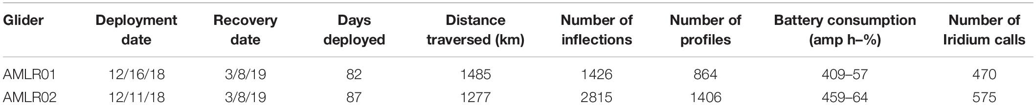
Table 1. Deployment and recovery details for gliders flown around the South Shetland Islands and northern Antarctic Peninsula during the austral summer of 2018/19.

FIGURE 1

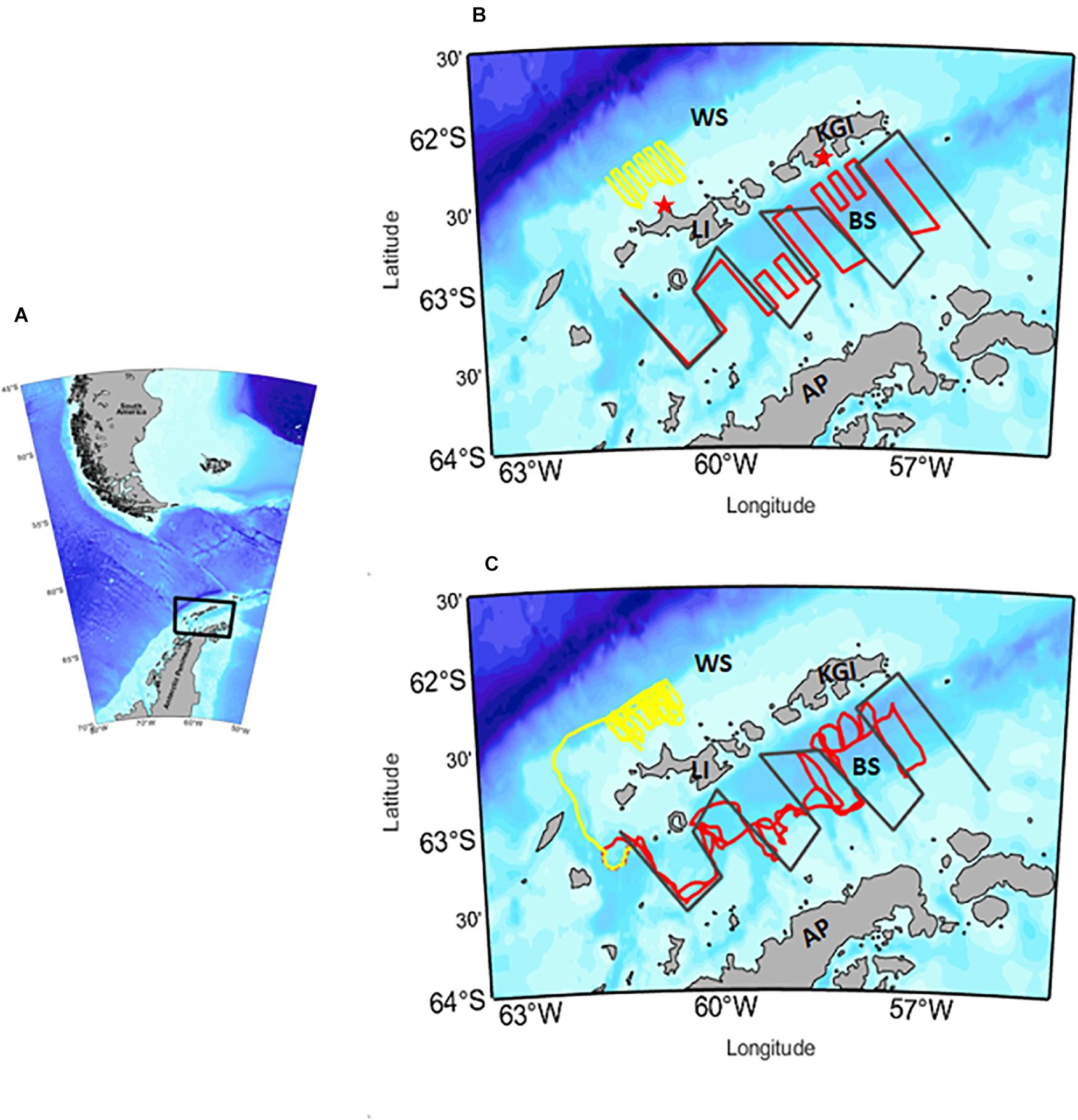
Figure 1. (A) Map of South America and the region surrounding the northern Antarctic Peninsula (AP) showing the region in which gliders were deployed (black box). (B) Map showing planned track lines of acoustically-equipped gliders deployed from mid-December 2018 to mid-March 2019 in two areas: the West Shelf (WS) off Livingston Island (LI; yellow) and the Bransfield Strait (BS; red). Planned track lines for previous ship-based surveys in the Bransfield Strait are illustrated as gray lines. Red stars indicate the locations of U.S. AMLR field camps at Cape Shirreff, LI and in Admiralty Bay, King George Island (KGI), where krill were sampled from penguin diets and used to construct length-frequency distributions. (C) Actual paths of gliders in a restricted area on the WS and in the BS, with planned track lines for previous ship-based surveys in Bransfield Strait for reference (gray lines). Repeat small-scale surveys were conducted in the restricted area (yellow lines) by the glider named AMLR02, and a single out-and-back survey of the BS (red lines) was conducted by AMLR01.

Glider Configuration and Basic Sampling

The U.S. AMLR Program developed a standard glider configuration for long-duration fisheries acoustics missions (Figure 2). Our gliders are Slocum G3 electric gliders manufactured by TWR; the vehicles are rated to 1000 m, with longer hull sections specifically designed to increase their volume and contain the instruments and batteries needed for extended missions (∼90–120 days with 20% power reserve). These deep gliders use an 860-mL oil-filled pump and diaphragm to change the buoyancy of the glider and thereby initiate dives and climbs. The gliders have a volume of approximately 88 L, are 2.7 m long, and weigh approximately 90 kg in air. The gliders were equipped with single-use lithium primary batteries that delivered 870 amp-hours of energy at 14.8 V to power the buoyancy pump, navigational instruments, and all science sensors.

FIGURE 2

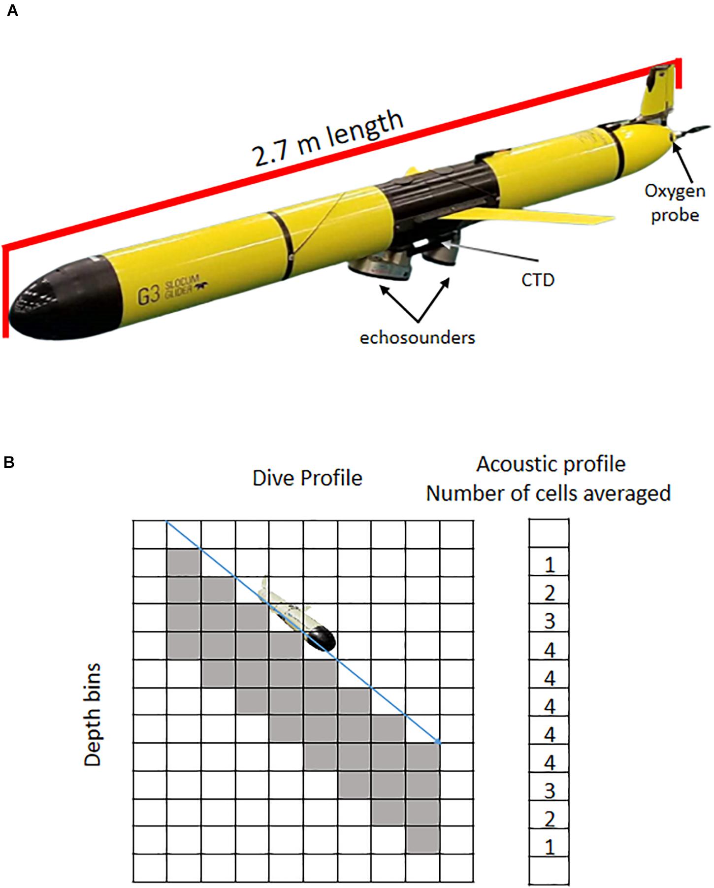
Figure 2. (A) Standard glider configuration illustrating the size and payload of U.S. AMLR gliders. The three frequency Acoustic Zooplankton and Fish Profiler (AZFP) is mounted in an extended science bay, with Seabird CTD visible above it and the oxygen probe near the propeller. (B) Diagram illustrating the process for converting acoustic observations collected during a glider dive into an acoustic profile. Acoustic observations are collected from a fixed range below the glider and along its glide path. Processed acoustic data (1 × 1 m bins) are averaged at each depth to convert the dive profile into a vertical profile.

The science payload of our standard glider includes oceanographic and acoustics packages (Figure 2). The oceanographic package comprises a pumped conductivity, temperature, and pressure sensor (Sea-Bird Electronics Inc., CTD model 41); an optical sensor that measures chlorophyll-a fluorescence, optical backscatter, and colored dissolved organic matter (Sea-Bird Electronics Inc., ECO Puck Triplet FLBBCD-SLC); and an optode to measure dissolved oxygen (model 4831). The acoustic package comprises three single-beam, single-frequency transducers (38, 67.5, and 125 kHz) integrated into the glider’s science bay (Taylor and Lembke, 2017; Chave et al., 2018). The transducers are fixed to the glider at a 22.7° downward angle and have varying beam widths (38 kHz: 30° beam width; 67.5 kHz: 17° beam width; and 125 kHz: 7° beam width).

All science sensors were programmed to sample during dives only, from the surface to the maximum dive depth. The CTDs, ECO Pucks, and optodes sampled at 4-s intervals. We programmed the gliders to dive at 22.7° so that the acoustic transducers were directed normal to the sea surface while sampling (Figure 2). In general, we instructed the gliders to dive to 950 m and ascend when within 10–30 m of the seafloor, as determined from the onboard altimeters. In shallow water (<300 m), the gliders performed three full dive-climb cycles before completely surfacing. In deeper water (>300 m), two dive-climb cycles were completed. Upon surfacing, the gliders updated their positions via the Global Positioning System (GPS); connected via Iridium to TWR’s web-based piloting software [Slocum Fleet Mission Control (SFMC)]; transmitted files containing subsampled flight, navigational, and scientific data (although we were unable to transmit acoustic data); and received new instructions from our pilots. Glider positions underwater were calculated by dead reckoning between surface GPS fixes, and we limited the number of dive-climb cycles between each complete surfacing to minimize positional errors.

We configured the AZFPs to transmit pulses of 500 μs on all three frequencies at an interval of 5 s with one transmission (ping) during each interval. The AZFP fires sequentially, from the highest frequency (125 kHz) to the lowest frequency (38 kHz) with a delay of ∼0.138 s between frequencies. Acoustic data were recorded over a range of 100 m from the vehicle and digitized at 40,000 Hz.

Calibration of Acoustic Sensors

The AZFPs were calibrated twice: once prior to deployment (mid-June 2018) and once after recovery (in late July 2019). Calibrations were performed using a tungsten carbide sphere (12.7 mm diameter), following Foote et al. (1987) and Taylor and Lembke (2017), in a seawater tank with known temperature and salinity at the Southwest Fisheries Science Center (La Jolla, CA, United States). For calibration, each glider was suspended on a custom-made rig at an angle of 22.7° and lowered until the transducers were 1 m below the surface. The target sphere was suspended by monofilament line (4 lb test) looped through a monofilament cradle tied to contain the sphere (Foote et al., 1987). The sphere was suspended approximately 3–4 m from the transducers, avoiding the range (5 m) at which echoes from the tank walls and bottom might interfere with the calibration. We used the upper 10% of on-axis acoustic returns from the beam of each transducer to determine gains and offsets for calibration (Demer et al., 2015). We used the in situ salinity and water temperature data from the CTD aboard the glider to adjust the sound speed in calculations using the echosounders.

Piloting

We piloted the gliders via TWR’s web-based SFMC piloting software (v. 8.3.0-56) from the Southwest Fisheries Science Center and our pilots’ personal residences. As close as possible, the pilots instructed the gliders to transit predetermined sets of waypoints offshore of Cape Shirreff, Livingston Island and within the Bransfield Strait (Figure 1). These survey areas, respectively, cover an important foraging ground for land-based predators on Livingston Island, and an important krill-fishing ground in the southern Bransfield Strait (Watters et al., 2020). The pilots modified waypoints during deployment based on the progress of the gliders, environmental conditions (waves, winds, and currents), and navigational hazards (principally icebergs). Environmental data were examined daily, including oceanographic circulation fields served at http://oceansmap.maracoos.org/. Iceberg locations were extracted from geo-referenced RADARSAT imagery (provided by MDA Geospatial Services Inc. through an agreement with NOAA), other imagery served at https://www.polarview.aq/antarctic, and interpretive sea-ice maps provided by the NOAA National Ice Center (https://www.natice.noaa.gov/). Glider positions, environmental data, and the RADARSAT imagery (including iceberg positions) were imported into a custom QGIS (3.14) project to visualize the operational situation in near real time.

One glider (AMLR02) was deployed off Cape Shirreff on December 11, 2018, and the other glider (AMLR01) was deployed in the Bransfield Strait on December 16, 2018 (Table 1). AMLR02 flew 87 days, performed 1406 dives, and covered 1277 km (Table 1). This glider typically flew in relatively shallow water over the continental shelf, which was reflected in the greater number of dives made by this glider relative to the other. AMLR02 completed two small-scale surveys off Cape Shirreff, each one lasting about 20 days. Other missions (e.g., sampling off the shelf in deeper water) consumed most of the remaining sea days before AMLR02 transited to the recovery area in Bransfield Strait (Figure 1). The oxygen sensor on AMLR02 failed 6 days after the glider was deployed, and its altimeter failed on February 09, 2019. After the altimeter failed, we canceled a third small-scale survey off Cape Shirreff because we could not reliably fly the glider in shallow water.

AMLR01 flew for 82 days, performed 864 dives, and covered 1485 km. During its flight, this glider completed several transects across the Bransfield Strait and two small-scale surveys within the Strait. The first 350 dives completed by AMLR01 comprised the first pass through the Bransfield Strait, and we used the acoustic data collected during these dives to estimate krill density for this paper. Noise in the AZFP (post-cruise analysis identified this noise as the result of a failed connector within the AZFP) precluded using the data from the second half of AMLR01’s deployment to provide a second estimate of krill density in Bransfield Strait.

Target Identification and Krill Length-Frequency Distributions

Length-frequency distributions of krill are required to estimate biomass density. Unlike ship-based surveys that typically use targeted, systematic, or random net tows to identify acoustic targets and determine their LFDs, contemporaneous net sampling was not an integral component of our glider deployment. However, LFDs of krill sampled from the diets of land-based predators (birds and mammals) are often correlated with LFDs of krill sampled using nets (Reid and Brierley, 2001; Miller and Trivelpiece, 2007), although diet-based LFDs may be biased toward larger krill.

We used krill LFDs from penguin diets to represent the size distributions of krill ensonified by our gliders. For the surveys off Cape Shirreff, we combined measurements of krill sampled from the diets of gentoo (Pygoscelis papua) and chinstrap (Pygoscelis antarcticus) penguins, collected by gastric lavage, into a single LFD. For the Bransfield Strait, we measured krill lengths from spilled prey boluses found within gentoo penguin colonies near our field camp on King George Island. All diet samples were collected during January 2019, and the foraging distributions of penguins breeding at both sampling locations overlapped portions of the areas surveyed by the gliders.

We compared estimates of biomass density based on LFDs from predator diets to estimates based on LFDs from net tows conducted during a multi-ship survey (Macaulay et al., 2019) conducted between December 2018 and March 2019. We used size compositions from net tows conducted within the areas surveyed by our gliders. Krill LFDs from these net-based data were smoothed with five-point running averages to reduce variability from measurement error.

Data Analysis—Glider Data

After recovery, data recorded by both gliders were downloaded and quality-controlled using the SOCIB Glider toolbox v 1.31 (Troupin et al., 2016). This toolbox is freely available MATLAB code developed to automate the processing of glider data. Data processing occurs in a number of steps, the first of which links time stamps from the flight and science computers onboard the glider with positions from consecutive GPS fixes. Subsequently, science and navigation data are further processed and quality-controlled through application of several filters and offsets. The processed navigation data (time, latitude, longitude, pitch, and roll) were extracted and linked, again by time stamp, to data collected by the AZFP, which operates with a separate computer and clock.

The gliders collected acoustic data during discrete, oblique dives through the water column. This sampling strategy differs from typical ship-based acoustic surveys, during which echosounders continuously collect data along transects and over a fixed range of depths relative to the water surface. Without considering the beam angles of the transducers, the acoustic targets ensonified by a glider during its dive occur within the polygon defined by the dive angle of the vehicle and the effective range of the acoustic instruments (Figure 2). In the case of gliders, the smallest identifiable patch length is dependent on the dive angle and interval between dives (Guihen et al., 2014). We flew our gliders with relatively constant dive angles (target angle of 22.7°). Therefore, the horizontal distance traversed during each dive-climb cycle and the interval between dives was primarily dependent on dive depth, with increased horizontal sampling resolution when dives were shallower and thus more frequent.

We used Echoview (Echoview Software Pty. Ltd., v 11.0) to process raw acoustic data that were linked to the glider navigation data by time stamp. Data collected within the first three meters from the transducer face were removed, as well as those within five meters of the seafloor. Data where a glider was diving at an angle less than 10° or greater than 30° were also removed. Raw acoustic data from each frequency were cleaned using Echoview’s Background Noise Removal (De Robertis and Higginbottom, 2007), Impulse Noise Removal, and Transient Noise Removal (Ryan et al., 2015) algorithms. Once cleaned, mean volume backscattering strength (MVBS or ${\overline{S}}_v$, dB) and area backscatter coefficient (ABC or s_a, m² m^–2) from each frequency were exported in 1 m × 1 m bins for further processing in MATLAB. We treated each dive as a sample, and generated dive-specific profiles of acoustic backscatter by averaging the acoustic data within the depth bins ensonified during each dive (e.g., Figure 2). We call these profiles because the averaging was horizontal, resulting in vertically-resolved estimates of MVBS and ABC. These profiles of MVBS and ABC were used to calculate biomass density. In general, our treatment of the acoustic data collected by the gliders was akin to the way in which oblique net hauls are used as point estimates of an organism’s density within a survey area. Our approach is not dependent on sampling a fixed number of transects nor entire swarms of krill.

Krill Identification Methods

We used dB differencing methods (Madureira et al., 1993) to limit our estimates of MVBS and ABC to those of krill. Target strengths of krill from 10 to 65 mm were calculated for all three frequencies using the full stochastic distorted-wave Born approximation (SDWBA) model assuming a normal distribution of orientation angles for krill with a mean of −20° and a standard deviation of 28° (SC-CAMLR, 2010). Typically, differences between volume backscattering strengths (ΔS_v) at either two (120 minus 38 kHz) or three frequencies (120 minus 38 kHz, and 200 minus 120 kHz) are used to identify krill from other acoustic scatterers (Reiss et al., 2008; Fielding et al., 2014). The two-frequency algorithm assumes that the ΔSv(120 – 38) of krill echoes fall within 0.69–16.86 dB (see Fielding et al., 2014). The mask for the ΔSv(125 – 38) for our frequencies is 0.02–17.9 dB. Because of problems with the 38 kHz echosounder (see below), we also calculated a two-frequency algorithm with ΔS_v computed from returns at 125 minus 67.5 kHz; this produced a krill mask between −3.4 and 8.98 dB. We note that two-frequency algorithms can erroneously classify krill swarms when other scatterers including copepods and fishes without swim bladders are present in the water column (Fallon et al., 2016).

Finally, we adapted the shoal analysis and patch estimation system (SHAPES) (Coetzee, 2000) to estimate krill biomass density for each glider survey using parameters close to those of a previous glider survey of krill in the Weddell Sea (Supplementary Data; Guihen et al., 2014). Given the challenges of using the two-frequency dB differencing approach (Madureira et al., 1993, see below), we used these estimates to examine variability attributable to the method by which krill were discriminated from other scatterers.

The biomass density of krill ρ_w (g m^–2) for each dive profile was calculated as

$${\mathrm{\rho }}_w=s_a\times \left(\sum _i{f}_i{w}_i\right)/\left(\sum _i{f}_i\mathrm{\sigma }_{bs}{}_i\right)$$

where s_a is the area backscattering coefficient for krill (m² m^–2; computed after target identification and which represents the volume backscattering coefficient s_v integrated over 5–250 m within each profile; MacLennan et al., 2002). σ_bs is the backscattering cross-section (m²) of krill within the ith length bin according to the SDWBA model. f_i is the frequency of krill in each length bin, and w_i is the weight (g) of krill in each length bin using the length-to-weight equation of Hewitt et al. (2004).

The mean biomass density $\overline{{\mathrm{\rho }}_w}$ is obtained by averaging the ρ_w over all dive profiles, where N_d is the total number of profiles.

$$\overline{{\mathrm{\rho }}_w}=\frac{1}{N_d}\sum _{n=1}^{N_d}{\mathrm{\rho }}_{w,n}.$$

We recognize that a number of different methods may be used to estimate the biomass density and its variance, but exploring such alternatives is beyond the scope of this paper.

Data Analysis—Previous Survey Results

To provide context for the interpretation of the biomass densities we estimated using gliders, we compared our results to those from other acoustic surveys in three ways. First, we extracted ship-based estimates of krill density from the U.S. AMLR Program’s survey database. These previous estimates are for a relatively large area encompassing those surveyed by the gliders (Reiss et al., 2008), and cover the period from 1996/97 through 2010/11. These previous estimates are quality-controlled, derived from daytime acoustic data integrated over 1 nmi and approximately 10–15 to 250 m depth, and based on application of the SDWBA and dB differencing of returns at three frequencies (38, 120, and 200 kHz). Biomass densities were estimated from the 120 kHz data; data from the other two frequencies were used for target identification. We considered all previous density estimates from the West Shelf (the area immediately north of Livingston and King George Islands, Figure 1) and the Bransfield Strait as “broad-scale” estimates of krill density. We subsetted the data previously collected from the West Shelf to estimate krill densities within a restricted polygon overlaying the continental shelf near Cape Shirreff, Livingston Island (Figure 3). We also compared glider-based estimates of krill density near Cape Shirreff to those from three nearshore surveys conducted during 2005–2007 (Warren et al., 2009) and within the boundaries of our glider survey (Figure 3). Comparisons to these various, previous density estimates provide context for interpreting the results of our glider surveys.

FIGURE 3

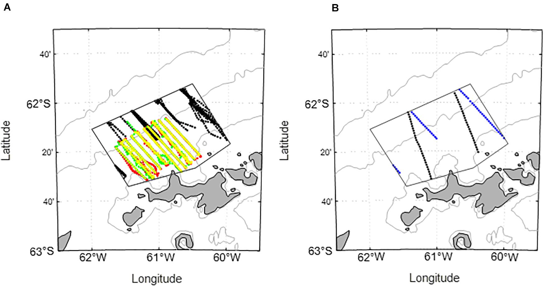
Figure 3. Bathymetric charts (250, 1000, and 3000 m isobaths) of the West Shelf illustrating the overlap of ship-based surveys with the area sampled by a glider during 2019/19. (A) Black points indicate coverage by previous, broad-scale surveys conducted by the U.S. AMLR Program within the restricted polygon subsequently sampled by a glider. Colored points represent the data collected during three [2005 (red), 2006 (green), and 2007 (yellow)] nearshore surveys. (B) Coverage by a multi-ship acoustic survey conducted during 2018/19 within the polygon contemporaneously sampled by a glider. Black points are from a January 19 transit by one ship, and blue points are from a March 05 transit by a second ship.

Second, we extracted acoustic data from a regional-scale multi-ship survey (Macaulay et al., 2019) that was temporally coincident with our glider surveys off Cape Shirreff (Figure 3) and in the Bransfield Strait. In Macaulay et al. (2019), a shoal analysis and patch estimation system (SHAPES) approach (Coetzee, 2000) was used to discriminate krill from other scatterers, and then biomass density was calculated at 120 kHz for each nautical mile of ship track (Macaulay et al., 2019). From the coincident ship survey over the West Shelf, we extracted data that were sampled within the same restricted polygon used to subset the acoustic data previously collected during U.S. AMLR ship surveys. It should be noted, however, that coverage of the restricted polygon during the multi-ship survey was fortuitous and not planned; ship-based coverage off the area near Cape Shirreff during 2018/19 was not optimized for comparison to the glider data. We calculated the biomass densities in the Bransfield Strait for the area where our glider survey and the multi-ship survey overlapped. Glider-based biomass densities were calculated using separate LFDs from predators and net tows performed as part of the multi-ship survey to examine variability attributable to how length-frequency data were sampled during the glider survey.

Results

Glider Stability

Excessive variability in vehicle roll and pitch can greatly impact acoustically-derived biomass estimates, but our gliders were relatively stable throughout their deployments. The gliders did not exhibit excessive roll, either during descent or ascent, and were always within about 1° of neutral. In general, pitch angles during dives were manageable and less than 1–2° from the target angle of 22.7°. There is some evidence that the dive angles of both gliders shoaled about 1° with increasing depth; this was probably a consequence of ballasting the vehicles for surface densities, and the relatively high H-moment (10) of the gliders as configured.

Krill Length Distributions

The LFDs of krill off Cape Shirreff and in Bransfield Strait were similar and unimodal (Figure 4). Krill from the diets of penguins foraging off Cape Shirreff were about 5 mm longer (mean = 48 mm) than krill eaten by penguins foraging in Bransfield Strait (mean = 43 mm). The LFDs for krill collected from net tows conducted during the multi-ship survey were similar to the LFD from penguins that foraged in the Bransfield Strait, but the mode was 2 mm larger (Figure 4). For the restricted polygon on the West Shelf, we only considered krill LFD from the two net tows made during the multi-ship survey. Krill from these trawls were substantially larger (mean = 51 mm) than krill in the diets of penguins that foraged off Cape Shirreff.

FIGURE 4

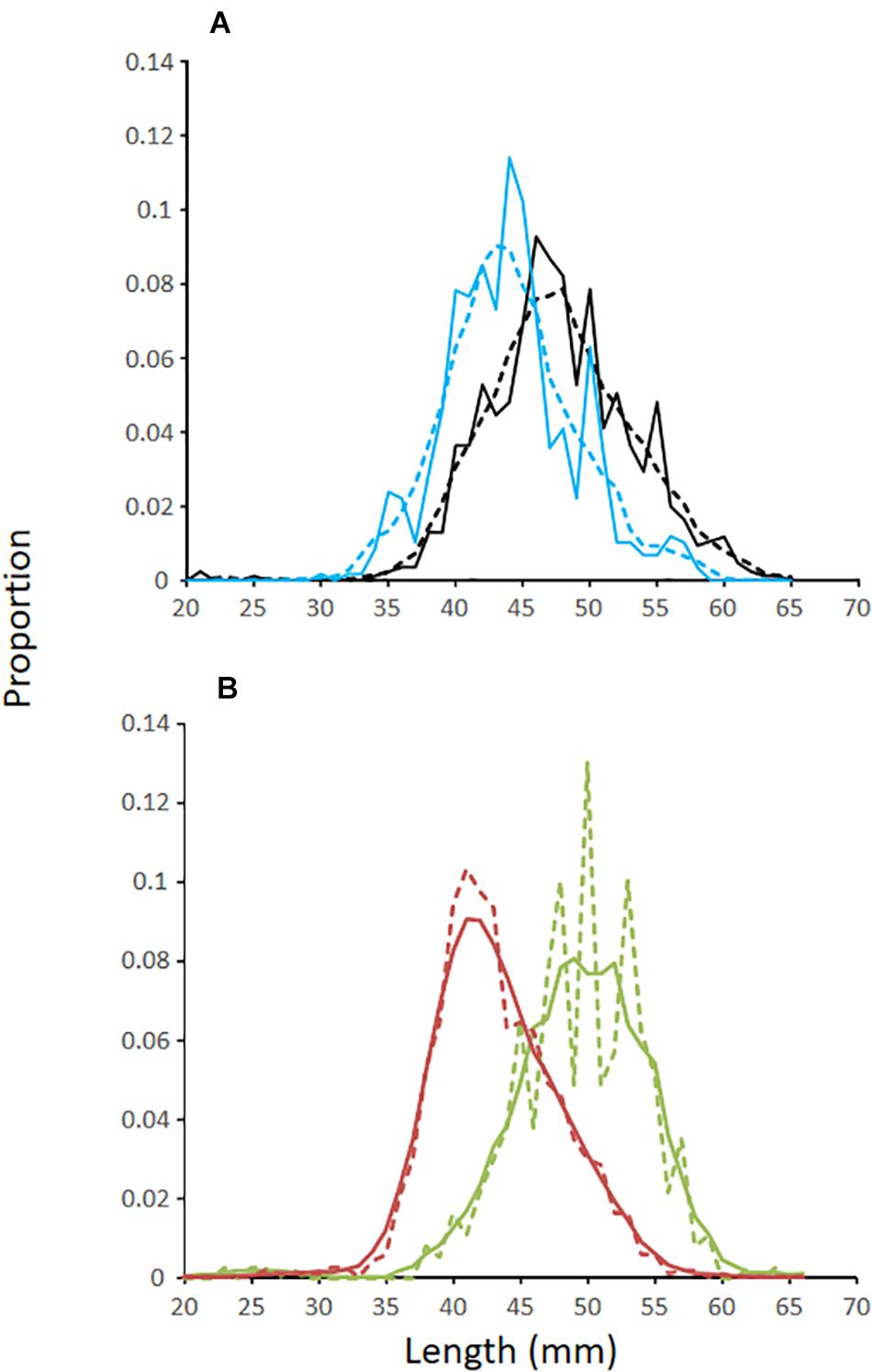
Figure 4. (A) Length-frequency distributions of Antarctic krill from (A) the diets of penguins foraging off Cape Shirreff (black lines) and King George Island (blue lines) during the austral summer of 2018/19. (B) Length-frequency distributions of krill from net tows conducted during ship-based surveys in 2018/19 where red lines represent data from the Bransfield Strait and the green lines represent data collected on the West Shelf and within the restricted area surveyed by a glider. Solid lines are raw data, and dashed lines are smooths based on a five-point running average.

Glider-Based Acoustic Data

Both gliders detected krill throughout their deployments. Patches of krill were observed throughout the upper 250 m of the water column, and these patches were most visible at 67.5 and 125 kHz. Returns at 38 kHz were extremely weak, even in locations where the other transducers demonstrated that krill were relatively concentrated. Very few krill aggregations were found at depths > 500 m (when such depths were sampled) or associated with the bottom. In fact, only two swarms were found deeper than 250 m.

The spatial patterns of krill biomass density varied between the two small-scale surveys on the West Shelf off Cape Shirreff (Figure 5). Krill were found over the shelf during both surveys but were highly concentrated between two canyons during the first survey and less concentrated between the canyons during the second survey. In Bransfield Strait, biomass density was highest in areas with bathymetric variability. Less biomass was found in deeper water; however, piloting the glider to avoid a large iceberg precluded sampling some deeper areas of the Bransfield Strait.

FIGURE 5

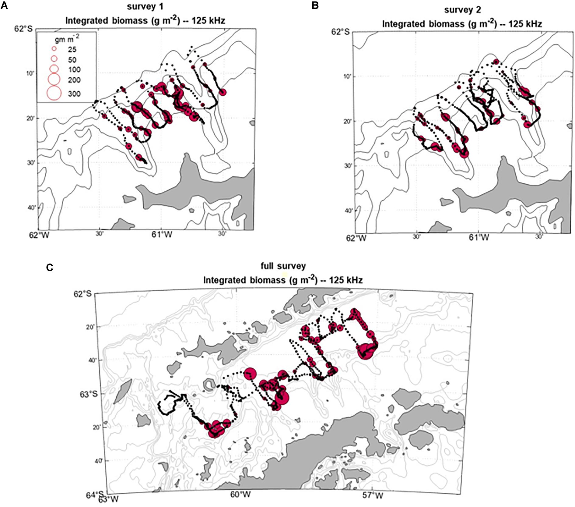
Figure 5. The spatial distribution of krill biomass density (g m^–2) at 125 kHz. Bubbles represent dives converted to profiles (as in Figure 2) and integrated over 5–250 m. The distances between points are a function of dive depth (deeper dives are farther apart) and whether each vehicle’s forward progress was hampered or enhanced by currents. The top two panels illustrate results from the two small-scale surveys flown over the West Shelf off Cape Shirreff from (A) mid-December 2018 to mid-January 2019 and (B) mid-January 2019 to mid-February 2019 (B). (C) Biomass density in Bransfield Strait from mid-December 2018 to mid-January 2019. Bathymetric contours are 150, 1000, and 3000 m.

Application of the dB-differencing method using the 125 and 38 kHz data produced a distribution of ΔS_v that was different from what would be predicted from the SDWBA model (Figure 6). The observed range of ΔS_v using 125 and 38 kHz was about −19.01 to 35.92 dB, with a mean dB difference of 17.02, which is at the very high range of dB differences attributed to krill in most studies (2–16 dB), suggesting a problem with one of the echo-sounders. dB differences between our observations at 125 and 67.5 kHz produced a distribution of ΔS_v that was consistent with predictions from the SDWBA model and ranged between −22.16 and 22.37 dB with a mean difference of 3.34 dB (Figure 6). Since dB differences between 125 and 38 kHz were not consistent with expectations from the SDWBA model while those between 125 and 67.5 kHz were consistent, we concluded that the 38 kHz echosounder was not functioning correctly. Therefore, we used the latter differences as a mask for krill, and applied a threshold filter to the total backscatter data, setting MVBS values < −80 dB to zero and estimating krill biomass density with observations recorded at 125 kHz.

FIGURE 6

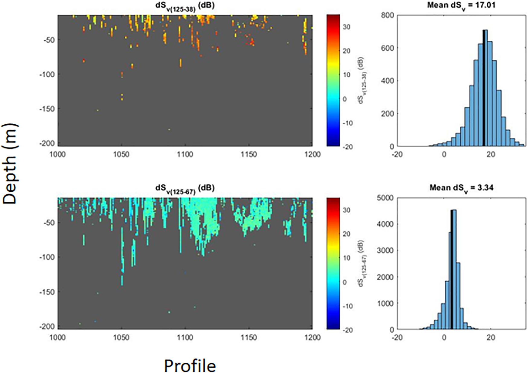
Figure 6. Decibel (dB) differences between acoustic returns collected by AMLR02 during austral summer 2018/19. The upper left panel shows differences in volume backscattering strength (dSv) for, approximately, the standard two-frequency algorithm for identifying krill targets (125 kHz minus 38 kHz). The upper right panel shows the histogram of the dB differences (blue bars) and mean dB difference (black reference line) for this algorithm. The lower left panel shows differences in volume backscattering strength for a krill-identification algorithm using differences between returns at 125 and 67.5 kHz, and the lower right panel shows the distribution of dB differences (blue bars) and mean dB difference (black reference line) for this alternative target-identification algorithm.

Biomass Estimates

Glider-Based Estimates

Glider-based estimates of krill biomass density varied between survey areas and over time (Table 2). During the two small-scale glider surveys starting in December 2018 and January 2019 off Cape Shirreff, we, respectively, estimated biomass densities of 110.6 and 55.3 g⋅m^–2. In Bransfield Strait, we estimated a mean biomass density of 106.7 g⋅m^–2 during the single survey that could be accomplished between mid-December 2018 and early January 2019.

TABLE 2

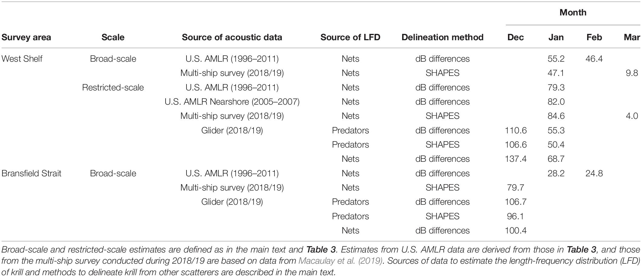
Table 2. Estimates of the mean biomass density (g m^–2) of krill over the West Shelf and in the Bransfield Strait.

General Comparisons With Previous Ship-Based Surveys

Off Cape Shirreff, glider-based estimates of krill density at 125 kHz were within the range of densities obtained from previous, ship-based surveys conducted by the U.S. AMLR Program (Tables 2, 3). Off Cape Shirreff, previous biomass densities ranged from 1.4 to 141.9 g⋅m^–2 during January and 0.4 to 126.2 g⋅m^–2 during February. When data from the previous ship surveys were restricted to the areas sampled by the glider, biomass density off Cape Shirreff ranged from 0.6 to 239.6 g⋅m^–2, suggesting that biomass estimates from observations made on the shelf could be higher than those that combine observations from the shelf and deeper water. Indeed the nearshore ship surveys from 2005 through 2007, that fully encompassed the areas sampled by the glider, indicated higher biomass densities than the broad scale surveys in two of the three years, ranging from 56.5 to113 g⋅m^–2 (Table 3). In general, the glider-based estimates of krill density were more similar to the restricted-area estimates and those from nearshore surveys. The relatively high biomass densities recorded in the restricted area and during the nearshore surveys probably reflect the concentration of krill on the continental shelf.

TABLE 3

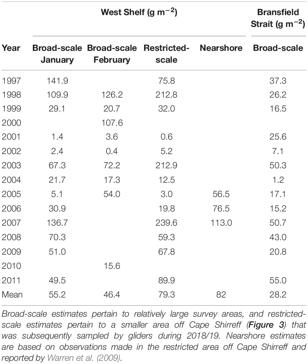
Table 3. Previous estimates of the mean biomass density (g m^–2, rounded to the nearest decimal point) of krill over the West Shelf and in the Bransfield Strait developed from ship-based acoustic surveys conducted by the U.S. AMLR Program.

In contrast to results from the survey area off Cape Shirreff, the glider-based estimate of krill density in Bransfield Strait was very different than estimates from previous surveys (Tables 2, 3). In fact, between 1996 and 2011, biomass densities from 13 broad-scale, ship-based surveys in Bransfield Strait ranged from 1.2 to 55 g⋅m^–2, but our glider-based estimate of krill density in the strait during 2018/19 was about twice (106.7 g⋅m^–2) the maximum historical density.

Comparison With Contemporaneous Ship-Based Surveys

We made several comparisons between density estimates from the contemporaneous multi-ship survey (Macaulay et al., 2019) and those from our gliders. We selected ship data from the West Shelf and Bransfield Strait that were geographically coincident with our glider data. On the West Shelf, two ships sampled within the restricted area surveyed by our glider: one during mid-January and another in early March (Table 2). In January, the mean biomass density from the first ship was 84.6 g⋅m^–2, which was between our glider-based estimates for December (110.6 g⋅m^–2) and January (55.3 g⋅m^–2). The ship-based density estimate for the restricted area during January was also intermediate to our glider-based estimates when we used the LFD from the ship to estimate biomass density from the glider and when we used the SHAPES algorithm to delimit krill observed by the glider (Table 2). By March, sampling by a second ship indicated that krill density had substantially decreased in the area off Cape Shirreff (Table 2). In the Bransfield Strait, our glider-based estimates of biomass density were greater than the ship-based estimate, again regardless of whether we applied the ship-based krill LFD to our glider data or used the SHAPES algorithm to delimit krill from other scatterers observed by the glider (Table 2). In general, the alternative LFDs (based on predator diets or net tows) and methods of delimiting krill from other scatterers (dB differencing or SHAPES) had relatively small effects on the differences between contemporaneous, ship- and glider-based estimates of krill density. Furthermore, our approach of using dB differences between returns at 125 and 67.5 kHz (as opposed to the more common approach of using differences between returns at 120 and 38 kHz) had a relatively small impact on our results.

Discussion

The use of gliders and other autonomous vehicles for fisheries research has been contemplated for some time (Fernandes et al., 2003), but implementing full programs (as opposed to pilot projects) that rely on such vehicles for assessing the status and trends of economically and ecologically important taxa is just commencing (Meinig et al., 2015). In this study, we successfully deployed two gliders, equipped with multi-frequency echosounders, to transition from a purely ship-based survey program to one that is primarily glider-based and autonomous. We plan to continue this effort in the future.

Although gliders and other autonomous vehicles have been deployed in the Antarctic for many years, there have been relatively few attempts to use acoustically-equipped vehicles to survey zooplankton and krill. Brierley et al. (2002) used an Autosub to demonstrate that krill were concentrated in a band near the sea-ice edge. More recently, Ainley et al. (2015) used a glider carrying a single-frequency echosounder (120 kHz) to examine relationships between foraging penguins and the distribution of meso-zooplankton in the Ross Sea. Saba et al. (2018) deployed a glider with a multi-frequency (200, 120, and 38 kHz) acoustics package for a few weeks in the Ross Sea to examine krill distributions. Guihen et al. (2014) conducted two short (65 and 14 h) glider deployments to compare glider-based estimates of krill density with those from a ship using a 120-kHz echosounder. Although the dataset collected by Guihen et al. (2014) is extremely small, the team showed that the glider-based estimates of krill density were generally comparable to those from the ship. We have attempted to extend these previous efforts in several ways, including by surveying at spatial scales that are more typical for fisheries surveys, applying LFDs from diet samples, and using a dB differencing approach to delineate krill from other scatterers observed by the gliders.

A number of concerns regarding the sampling of patchily-distributed organisms, like krill, using acoustically-equipped gliders have been raised in both field (Guihen et al., 2014) and simulation (Guihen, 2018) studies. These concerns may influence perceptions regarding the capacity for gliders to meet the requirements of fisheries assessment. Perhaps the greatest perceived limitation of using gliders for fisheries research is the inability of a single vehicle to sample quickly enough to consider the survey sufficiently comprehensive in scale to ensure that the population or biological process of interest is appropriately sampled. In general, researchers attempt to complete synoptic surveys quickly, within a period of time during which the density or abundance of the target organism can be assumed to have been relatively constant. The slow speed of a glider relative to that of a ship thus suggests that glider surveys will be synoptic over smaller areas than those of ships. In general, our gliders completed surveys off Cape Shirreff (11 nominal transects in a survey area of about 1300 km²) and in the Bransfield Strait (eight nominal transects in a survey area of about 24,000 km²) over the course of 20–25 days. Historically, the ship-based surveys conducted by the U.S. AMLR Program were completed in less than 20 days and covered a much larger area (25 nominal transects in a survey area of about 128,000 km²). Glider surveys can be as synoptic as ship surveys simply by increasing the number of vehicles simultaneously deployed within the study area and distributing the locations at which each glider starts sampling. Deploying and distributing multiple gliders during a single survey also allows multiple locations to be sampled simultaneously and opens possibilities, for example, to collect observations across a hierarchy of spatial scales. We intend to deploy multiple gliders during future krill surveys.

In a modeling study, Guihen (2018) argued that significant biases in swarm size determination, and therefore in the echo-integration using the SHAPES approach, could occur when gliders sample in the direction of and their forward velocity is aliased by prevailing currents and because gliders sample only part of the water column. We sampled mostly perpendicular to the prevailing circulation, albeit imperfectly. This is the same approach used to minimize the probability that acoustic transects will resample the target species during ship-based surveys. Although some analysts apply the SHAPES algorithm to ship-survey data for estimating the type, number, and density of krill in patches and then echo-integrate the observed aggregations, our approach was to generate point-based estimates of biomass density, generated from profiles characterized by diving gliders. Further, by generating discrete profiles in which observed densities are averaged within depth bins, any oversampling within a dive should reduce biases when the goal of the study is to estimate biomass rather than to examine the spatial structure of meso-zooplankton schools or swarms.

Given that gliders only sample a small fraction of the water column, undersampling krill swarms, and thus underestimating density, is a potential concern. Simulation studies, where a virtual glider is flown through a time series of ship-based acoustic data, with a variable number of gliders, number of dives, and depth of dives will be useful to determine whether the sawtooth flight pattern of gliders introduces bias and whether long-term trends in biomass density comparable to those from ship-based surveys can be recovered.

Target Identification

The dB difference approach to classify and quantify acoustic targets for echo-integration uses differences in volume backscatter between returns at two or more frequencies. This approach works because animals with different acoustic properties will scatter acoustic energy differently based on their material properties, size, and behavior (Madureira et al., 1993; McGehee et al., 1998). For krill, two- (e.g., 120 minus 38 kHz) or three-frequency (e.g., 200 minus 120 kHz and 120 minus 38 kHz) dB differencing is often applied (e.g., Reiss et al., 2008; Fielding et al., 2014). We attempted to apply two-frequency dB differencing using returns at 125 minus 38 kHz, without success. Pre- and post-deployment calibrations of our 38-kHz instruments were the same, so it is unclear why these echosounders performed poorly. In contrast, the mean dB difference between the 125 and 67.5 kHz transducers was within the range, as expected from the SDWBA model, attributed to krill between 30 and 50 mm. We thus used this dB-difference mask to delineate krill from other scatterers. We acknowledge that Fallon et al. (2016) demonstrated that, in some cases, differences of 2–12 dB (or even 2–16 dB) were not adequate to separate krill from other scatterers like mackerel icefish (Champsocephalus gunnari) around South Georgia. Both krill and icefish are essentially Rayleigh scatterers and the wide dB difference between 38 and 125 kHz could include both species (and others), overestimating estimates of krill density. A similar challenge could result from using differences between 125 and 67.5 kHz. We tested, albeit partially, whether we may have included other scatterers in our estimates of krill density by using the SHAPES algorithm (Coetzee, 2000) to classify swarms of krill. Our results from the SHAPES approach were very similar to those from the dB differencing approach, suggesting that we did not include substantial amounts of other scatterers when we used the latter. While the goal of this paper was not to compare methods for estimating biomass densities, the similarity of our results using SHAPES and dB differencing is worth noting. Of course, in other areas and for other species that either do not swarm or occur in relatively continuous aggregations, the SHAPES algorithm may not be appropriate for estimating density from glider-based surveys.

Target Validation

Acoustic surveys typically include net tows to collect targets in the water column, validate that acoustic energy is attributed to the species of interest, and generate LFDs to convert acoustic energy to biomass. Net tows may not be feasible during glider surveys if, as in our case, the gliders operate independently while the deployment and recovery vessel conducts other tasks. Previous work (Reid and Brierley, 2001; Miller and Trivelpiece, 2007) has shown that the LFDs of krill in the diets of seabirds can reflect those of krill collected in nets, and we leveraged this finding for our glider surveys. We did not find a consistent bias toward larger krill in the LFDs from diets of penguins as compared to those from net tows conducted in overlapping areas and in the same month. On the West Shelf, the net-based LFDs indicated larger krill than those of penguins, while in the Bransfield Strait, the penguin LFDs indicated larger krill. The alternative LFDs had expected effects of increasing our glider-based estimates of biomass density when LFDs indicated larger krill. In years when the true LFD of the krill population is bi-modal, glider-based estimates of krill density which depend on LFDs from predators that select for larger krill would be biased. These results emphasize the general need to understand potential sources of error and find ways to develop unbiased LFDs of target scatterers. In other ecosystems, the diets of marine mammals and seabirds have also been shown to track recruitment, demographic patterns, and community structure of fishes and zooplankton, suggesting that diets of mammals and birds can be useful to inform acoustic models (Cairns, 1992; Barrett et al., 2007) where gliders might be deployed to monitor meso-zooplankton populations.

Of course, it is best to directly validate the zooplankton targets and their lengths in some manner. Because krill are found in the upper 100 m of the water column during the day, it may be possible to validate krill targets using simple camera technology. For example, low-light cameras have been deployed on penguins and fur seals to examine their feeding patterns, and these cameras commonly record krill (U.S. AMLR Program, unpublished data). Integrating cameras into gliders may be an easy and relatively inexpensive way to provide visual validation of acoustic targets as the vehicles transit through layers or patches of the target species. In other ecosystems, where multiple taxa may be more common, more elaborate cameras (e.g., Ohman et al., 2019) might provide target-validation data.

Biomass Estimation and Variability

Comparisons to contemporaneous data collected by the multi-ship survey showed that glider-based biomass densities bracketed a ship-based estimate on the West Shelf but were higher than a ship-based estimate in Bransfield Strait (Table 2). In the Bransfield Strait, both the glider-based estimates of biomass density and that from the multi-ship survey conducted in 2018/19 were also substantially higher than estimates based on previous U.S. AMLR surveys (Tables 2, 3). Thus, in the Bransfield Strait, both the glider survey and the multi-ship survey indicated that krill biomass had, relative to a 15-year time series, increased in this area. Glider-based surveys seem clearly able to distinguish “high” (and probably “low”) years as well as ship-based surveys, and our results suggest that gliders can provide defensible estimates of biomass density.

Despite the comparability of our glider-based estimates of krill density to those estimated from ships during a single year, time series of glider-based estimates may not be directly comparable to those of ships for many reasons. These reasons include the standard problems of target strength estimation and target identification, but also reflect differences in how gliders sample and the potential for gliders to oversample locations where the vehicles are “trapped” by local circulation (e.g., tidal currents) and which may also cause the target species to aggregate or disperse. However, such issues can be addressed with thought to appropriate sampling designs. Also, time series of krill biomass developed using gliders will be internally consistent, and thus provide a relative index of biomass that can be useful for managing fisheries.

Survey Challenges

Properly designing a glider-based fisheries survey to estimate the biomass of a target species presents some challenges that have not been directly addressed in our study. The slow speed of the gliders compared to ships might require that more than a single glider be deployed to sample synoptically. This is an approach that has been used in ship-based surveys in the Antarctic (Hewitt et al., 2004; Macaulay et al., 2019) and for autonomous surveys using Saildrones in the Bering Sea (De Robertis et al., 2019). In this study, we deployed two gliders to cover two different areas of interest, at different spatial scales, but could easily have deployed more gliders without increasing the costs of ship-time necessary for deployment or recovery.

In this study, we have attempted to approximate the ship-based sampling designs of surveys conducted by the U.S. AMLR Program since the early 1990s. To estimate biomass and quantify uncertainty in our estimates from these surveys, we previously relied on a stratified random transect design (Jolly and Hampton, 1990). It is possible that the same design-based approach can be used for acoustic transects sampled by the gliders, especially when glider transects are fairly straight. However, the slow speed of gliders and their propensity to be affected by tidal and other circulation means that some areas can be oversampled when the vehicles cannot make forward progress (e.g., Figure 5). Developing appropriate approaches to address this issue will be important moving forward. For example, consecutive dives that are within a nominal spatial or temporal distance of each other could be subsampled prior to biomass estimation, or profiles can be filtered out of subsequent analyses if currents and tides slow a vehicle’s progress. However, it may be more holistic to apply geo-statistical approaches to estimating biomass and its variability across the survey areas. Such methods have been used in fisheries research (Petitgas, 1993), are becoming increasingly complex (Petitgas et al., 2017), and may also provide appropriate confidence intervals that will be useful to inform management (Petitgas, 1993; Thorson et al., 2015).

Given relatively recent deployment of acoustic instruments on gliders, avoidance of autonomous vehicles by meso-zooplankton has not been widely studied. However, it is a fundamental issue with ship-based acoustic surveys. We anticipate that relative silance of autonomous instruments will be unlikely to drive avoidance. However, a diving glider may be perceived as a diving predator, and krill are known to move away from predators. Such avoidance is visible during CTD casts from ships when the CTD descends through krill swarms. Investigation of avoidance is an important consideration for future studies, but, as happened with ships, the lack of data on avoidance should not hinder the deployment and use of gliders while that research is undertaken.

Various other factors also need to be understood to use gliders for fisheries surveys. For example, ship-based surveys often do not sample the upper 15–20 m of the water column because of each ship’s draft and the blanking distance (∼5 m) below the hull-mounted transducers. Gliders can begin to sample almost at the surface, and the blanking distance of the AZFP is just 3 m. We began acoustic sampling at a depth of 3 m, when the gliders were in a stable dive attitude, and the transducers were normal to the sea surface. We were able to sample much closer to the surface than during previous ship-based surveys. Thus, it will be important to consider the fact that there is a difference of about 5–10 m of additional data collected by the glider that could impact comparisons to ship-based data. Sampling closer to the surface could negatively impact the quality of glider data if gliders are susceptible to other sources of surface noise. For example, bubbles can contaminate acoustics data collected by ships in less than ideal conditions, and could also impact gliders. However, we did not observe evidence of bubble contamination in the acoustic data from the gliders, but identification and removal of any types of noise should be part of the processing.

Piloting Challenges

Our glider deployments during 2018/19 were not incident-free. The loss of the oxygen sensor did not impact the overall mission for AMLR02; however, the loss of the altimeter did. To protect AMLR02, the glider was piloted offshore to deeper water where the altimeter was not needed. There the vehicle continued to provide useful data on the distribution of krill at the shelf edge and at depths not normally sampled acoustically. The degradation and eventual loss of the AZFP on AMLR01, however, impacted its core mission. Because of current limitations in the integration of scientific instruments into glider payloads and the limitations (cost and bandwidth) of transmitting acoustic data via Iridium, we were unaware the AZFP had malfunctioned. Thus, we failed to retask the glider to collect other data that might have been prioritized had we known the primary mission failed. The large volumes of data collected by active (Guihen et al., 2014) and passive (Baumgartner et al., 2013) acoustic systems as well as various optical instruments (Ohman et al., 2019; Whitmore et al., 2019) cannot be quickly transmitted via Iridium. This limitation requires that manufacturers improve integration of scientific sensors with other glider computers, so that at least the performance of such instruments can be monitored. This limitation also suggests that more effort to process raw data onboard gliders without overly consuming available battery power, and then transmit summary data via Iridium, would also be valuable.

Challenges to piloting the gliders were due to currents, including tidal currents, in shallow areas and near bathymetric features, and the presence of a large (25 km length), tabular iceberg in Bransfield Strait. This iceberg required pilots to deviate from planned waypoints during the deployment of AMLR01. Further, in shallow water (<150 m), tidal flows often made piloting the gliders difficult, resulting in oversampling some locations. In places where freshwater produced buoyant plumes, piloting gliders was also difficult. Because of the configuration of the acoustic instruments on the ventral side of the glider, the AMLR gliders have high H moments (>9) and use large displacement (860 mL) pumps that are standard in the 1000 m Slocum G3 gliders from TWR. This combination is not ideal for quick movements in shallow water (e.g., the pump moves slowly and thus the glider’s angle of attack changes slowly), but is manageable with careful piloting.

There is a large effort underway to develop better methods for piloting gliders that directly incorporate information from numerical models (Carrier et al., 2019), share information between and among fleets or swarms of gliders (Bigus-Kwiatkowska et al., 2018), and adaptively sample and respond to the environment (Leonard et al., 2010). While some of these methods have progressed greatly over the years, gliders that travel at the same speeds as coastal currents seem likely to require hands-on piloting for the foreseeable future. The occurrence of other hazards like island-sized icebergs that themselves calve village-sized icebergs will also require continued diligence in polar environments. We employed a team of three pilots and two other science planners who worked together (with one pilot and one planner on duty at any given time) to share the workload over approximately 90 days of survey effort.

Power Consumption and Costs

Power consumption over the ∼90 days of our deployments was only 55–60% of the available energy (Table 1). This energy surplus provides the ability to ensure that if gliders cannot be recovered during planned recovery periods, the vehicles can remain at sea until a new opportunity arises and can be flown to locations where recovery is more feasible. The additional remaining power also provides an opportunity to add new sensors to the payloads of the gliders in the future or use the thruster if necessary.

Our choice to use electric gliders to conduct the surveys was based on a few important constraints ease of deployment, portability, relative cost, as well as duration and ability to withstand ice. The first three requirements were based on the goal that any instrument system deployed should be manageable by a small group with modest engineering capacity. Other instruments that are propeller driven do not have the endurance to be deployed for months at a time, while other surface instruments may interact unfavorably with the large amounts of ice in the Antarctic coastal and shelf environments.

A number of studies have evaluated the relative costs of gliders and autonomous platforms relative to those of ships (Schofield et al., 2007; Rudnick, 2016). In the Antarctic, where the transiting to study areas from ports of embarkation in gateway countries or bases on the continent can take several days, deploying autonomous platforms from ships of opportunity (e.g., supply, fishing, or tourist vessels) can result in substantial cost savings. Savings can also be had by purchasing only a few days of ship time on existing science cruises rather than funding entire ship-based surveys (as we have done). Deploying multiple gliders from any ship can also decrease the environmental footprint of ecosystem monitoring.

Conclusion

For a number of reasons (e.g., cost, staffing, and logistical challenges), we have replaced an annual ship-based survey with the use of long-duration, acoustically-equipped buoyancy gliders. As demonstrated here, the capability of autonomous instruments to collect acoustic data at a variety of spatial scales has been successfully demonstrated. There are certainly details to work through regarding appropriate statistical models for estimating confidence bounds around biomass densities estimated from glider-based acoustic surveys, determining how best to conduct temporally- and spatially-synoptic surveys, and addressing issues like avoidance and instrument sensitivity. The data that support annual assessments of the status of the Antarctic krill and related components of the ecosystem (krill-dependent predators) are usually collected during December to March and presented to the CCAMLR during July and October. Thus, recovery of gliders in late March will not necessarily lead to delays in presenting results to managers. However, if decision makers wish to manage in near real time, there could be delays in providing glider-based data to managers. One solution might be to process acoustic data onboard the gliders, and telemeter summary data via Iridium along with other scientific and flight data when the glider surfaces. This would require additional computing power, and might shorten the potential deployment periods, but could be useful in these circumstances.

Our work demonstrates that gliders can provide defensible estimates of the biomass of an important fishery resource. These estimates are comparable to those derived from ship-based surveys. Technological advances in battery efficiency, low-power scientific sensors, and vehicle flight and navigation will likely continue and ultimately increase the capability of buoyancy-driven gliders to provide ever greater quantities of richer, high-quality data. The utility of including gliders in observing systems is well-recognized (Handegard et al., 2013; Greene et al., 2014; Rudnick, 2016), and now this platform can be used to support fisheries surveys and assessments.

Data Availability Statement

The raw data supporting the conclusions of this article will be made available by the authors, without undue reservation.

Author Contributions

All authors listed have made a substantial, direct and intellectual contribution to the work, and approved it for publication.

Conflict of Interest

The authors declare that the research was conducted in the absence of any commercial or financial relationships that could be construed as a potential conflict of interest.

Acknowledgments

We thank our colleagues at the Rutgers University Center for Ocean Observing Leadership (COOL) Lab, especially David Aragon and Nicole Waite as well as Josh Kohut and Oscar Schofield. We also thank Ben Allsup and Chris DeCollibus and the team at Teledyne Webb Research, and Jan Buerman at ASL, Inc., for ensuring that our gliders were delivered in time, and for answering questions and providing solutions at all our hours of the day and night. We thank Observers and Members of CCAMLR, who conducted the multi-ship survey of krill during 2018/19. In particular, we thank the Association of Responsible Krill Harvesters (ARK) for the use of data collected by their contract ship. We thank Korea, in particular Seok-Gwan Choi, for permission to use the data from their March 2019 survey. We thank Kostiantyn Demianenko and the Institute of Fisheries and Marine Ecology and IKF LLC (Ukraine) for the use of their data. Finally, we thank our colleagues at the Institute of Marine Science in Norway, Bjorn Krafft and Gavin Macaulay, who collected data during the multi-ship survey under grants and contracts supported by the Norwegian Ministry of Trade, Industry and Fisheries (NFD, via project number 15208); the Institute of Marine Research (IMR); and the IMR project “Krill” (project number 14246). Additionally, we thank our partners at the U.S. National Science Foundation, and the contractors on the Antarctic Support Contract for all their help in deploying and recovering our gliders and continuing to ensure that our program goes off without a hitch. The NOAA National Ice Center provided the ice data that helped to safely pilot the gliders over the 3-month period. Finally, we thank our reviewers for their constructive comments.

Supplementary Material

The Supplementary Material for this article can be found online at: https://www.frontiersin.org/articles/10.3389/fmars.2021.604043/full#supplementary-material

References

Ainley, D. G., Ballard, G., Jones, R. M., Jongsomjit, D., Pierce, S. D., and Smith, W. O. Jr., et al. (2015). Trophic cascades in the western Ross Sea, Antarctica: revisited. Mar. Ecol. Progr. Ser. 534, 1–16. doi: 10.3354/meps11394

CrossRef Full Text | Google Scholar

Barrett, N., Seiler, J., Anderson, T., Williams, S., Nichol, S., and Hill, S. (2010). “Using an autonomous underwater vehicle to inform management of biodiversity in shelf waters,” in Proceedings of the OCEANS 2010 IEEE—Sydney, (New York, NY: IEEE), 146–151.

Google Scholar

Barrett, R. T., Camphuysen, C. J., Anker-Nilssen, T., Chardine, J. W., Furness, R. W., Garthe, S., et al. (2007). Diet studies of seabirds: a review and recommendations. – ICES J. Mar. Sci. 64, 1675–1691. doi: 10.1093/icesjms/fsm152

CrossRef Full Text | Google Scholar

Baumgartner, M. F., Fratantoni, D. M., Hurst, T. P., Brown, M. W., Cole, T. V. N., Van Parijs, S. M., et al. (2013). Real-time reporting of baleen whale passive acoustic detections from ocean gliders. J. Acoust. Soc. Am. 134, 1814–1823. doi: 10.1121/1.4816406

CrossRef Full Text | Google Scholar

Benoit-Bird, K. J., Patrick Welch, T., Waluk, C. M., Barth, J. A., Wangen, I., McGill, P., et al. (2018). Equipping an underwater glider with a new echosounder to explore ocean ecosystems. Limnol. Oceanogr. Methods 16, 734–749. doi: 10.1002/lom3.10278

CrossRef Full Text | Google Scholar

Bigus-Kwiatkowska, M., Fronczak, A., and Fronczak, P. (2018). Critical properties of unlimited gliding: unexpected flocking behavior driven by the exchange of information. Phys. Rev. E 97:2018.

Google Scholar

Brierley, A., Fernandes, P., Brandon, M., Armstrong, E., Millard, N., Mcphail, S. D., et al. (2002). Antarctic krill under sea ice: elevated abundance in a narrow band just south of ice edge. Science 295, 1890–1892. doi: 10.1126/science.1068574

PubMed Abstract | CrossRef Full Text | Google Scholar

Cairns, D. (1992). Bridging the gap between ornithology and fisheries science: use of seabird data in stock assessment models. Condor 94, 811–824. doi: 10.2307/1369279

CrossRef Full Text | Google Scholar

Carrier, M. J., Osborne, J. J., Ngodock, H. E., Smith, S. R., Souopgui, I. J. M. D., and Addezio. (2019). Multiscale approach to high-resolution ocean profile observations within a 4DVAR analysis system. Month. Weath. Rev. 147, 627–643. doi: 10.1175/MWR-D-17-0300.1

CrossRef Full Text | Google Scholar

Carvalho, F., Kohut, J., Oliver, M. J., Sherrell, R. M., and Schofield, O. (2016). Mixing and phytoplankton dynamics in a submarine canyon in the West Antarctic Peninsula. J. Geophys. Res. Oceans 121, 5069–5083. doi: 10.1002/2016JC011650

CrossRef Full Text | Google Scholar

Chave, R., Buermans, J., Lemon, D. D., Taylor, J. C., Lembke, C., DeCollibus, C., et al. (2018). “Adapting multi-frequency echo-sounders for operation on autonomous vehicles,” in Proceedings of the OCEANS 2018 MTS/IEEE Charleston, Charleston, SC. doi: 10.1109/OCEANS.2018.8604815

CrossRef Full Text | Google Scholar

Coetzee, J. (2000). Use of a shoal analysis and patch estimation system (SHAPES) to characterize sardine schools. Aquat. Liv. Resour. 13, 1–10. doi: 10.1016/s0990-7440(00)00139-x

CrossRef Full Text | Google Scholar

Cole, S. T., and Rudnick, D. L. (2012). The spatial distribution and annual cycle of upper ocean thermohaline structure. J. Geophys. Res. Oceans 117:C02027. doi: 10.1029/2011JC007033

CrossRef Full Text | Google Scholar

Davis, R., Eriksen, C., and Jones, C. (2002). “Autonomous buoyancy-driven underwater gliders,” in The Technology and Applications of Autonomous Underwater Vehicles, ed. G. Griffiths (London: Taylor and Francis), 37–58. doi: 10.1201/9780203522301.ch3

CrossRef Full Text | Google Scholar

Davis, R. E., Leonard, N. E., and Fratantoni, D. M. (2009). Routing strategies for underwater gliders. Deep Sea Res. 56, 173–187. doi: 10.1016/j.dsr2.2008.08.005

CrossRef Full Text | Google Scholar

De Robertis, A., and Higginbottom, I. (2007). A post-processing technique to estimate the signal-to-noise ratio and remove echosounder background noise. ICES J. Mar. Sci. 64, 1282–1291. doi: 10.1093/icesjms/fsm112

CrossRef Full Text | Google Scholar

De Robertis, A., Lawrence-Slavas, N., Jenkins, R., Wangen, I., Mordy, C. W., Meinig, C., et al. (2019). Long-term measurements of fish backscatter from Saildrone unmanned surface vehicles and comparison with observations from a noise-reduced research vessel. ICES J. Mar. Sci. 76, 2459–2470. doi: 10.1093/icesjms/fsz124

CrossRef Full Text | Google Scholar

Demer, D. A., Berger, L., Bernasconi, M., Bethke, E., Boswell, K., Chu, D., et al. (2015). Calibration of acoustic instruments. ICES Cooperat. Res. Rep. 326:133.

Google Scholar

Demer, D. A., and Conti, S. G. (2003). Validation of the stochastic distorted-wave, Born approximation model with broad bandwidth total target strength measurements of Antarctic krill. ICES J. Mar. Sci. 60, 625–635. doi: 10.1016/s1054-3139(03)00063-8

CrossRef Full Text | Google Scholar

Domingues, R., Kuwano-Yoshida, A., Cardon-Maldonado, P., Todd, R. E., Halliwell, G., Kim, H.-S., et al. (2019). Ocean observations in support of studies and forecasts of tropical and extratropical cyclones. Front. Mar. Sci. 6:446. doi: 10.3389/fmars.2019.00446

CrossRef Full Text | Google Scholar

Eriksen, C. C., Osse, T. J., Light, R. D., Wen, T., Lehman, T. W., Sabin, P. L., et al. (2001). Seaglider: a long range autonomous underwater vehicle for oceanographic research. IEEE J. Oceanic Engin. 26, 424–436. doi: 10.1109/48.972073

CrossRef Full Text | Google Scholar

Eriksen, E., Skjoldal, H. R., Dolgov, A. V., Dalpadado, P., Orlova, E. L., and Prozorkevich, D. V. (2016). The Barents Sea euphausiids: methodological aspects of monitoring and estimation of abundance and biomass. – ICES J. Mar. Sci. 73, 1533–1544. doi: 10.1093/icesjms/fsw022

CrossRef Full Text | Google Scholar

Fallon, N. G., Fielding, S., and Fernandes, P. G. (2016). Classification of Southern Ocean krill and icefish echoes using random forests. ICES J. Mar. Sci. 73, 1998–2008. doi: 10.1093/icesjms/fsw057

CrossRef Full Text | Google Scholar

Fernandes, P. G., Stevenson, P., Brierley, A. S., Armstrong, F., and Simmonds, E. J. (2003). Autonomous underwater vehicles: future platforms for fisheries acoustics. ICES J. Mar. Sci. 60, 684–691. doi: 10.1016/s1054-3139(03)00038-9

CrossRef Full Text | Google Scholar

Fielding, S., Watkins, J., Trathan, P. N., Enderlein, P., Waluda, C. M., Stowasser, G., et al. (2014). Interannual variability in Antarctic krill (Euphausia superba) density at South Georgia, Southern Ocean: 1997–2013. ICES J. Mar. Sci. 9, 2578–2588. doi: 10.1093/icesjms/fsu104

CrossRef Full Text | Google Scholar

Foote, K. G., Knudsen, H. P., Vestnes, G., MacLennan, D. N., and Simmonds, E. J. (1987). Calibration of acoustic instruments for fish density-estimation – A practical guide. J. Acoust. Soc. America. 83, 72–84.

Google Scholar

Freitas, F. H., Saldias, G. S., Goni, M., Shearman, R. K., and White, A. E. (2018). Temporal and spatial dynamics of physical and biological properties along the endurance array of the california current ecosystem. Oceanography 31, 80–89. doi: 10.5670/oceanog.2018.113

CrossRef Full Text | Google Scholar

Ghani, M. H., Hole, L. R., Fer, I., Kourafalou, V. H., Wienders, N., Kang, H., et al. (2014). The SailBuoy remotely-controlled unmanned vessel: measurements of near surface temperature, salinity and oxygen concentration in the Northern Gulf of Mexico. Meth Ocean 10:1. doi: 10.1016/j.mio.2014.08.001

CrossRef Full Text | Google Scholar

Goodrich, C. S. (2018). Sustained Glider Observations of Acoustic Scattering Suggest Zooplankton Patches are Driven by Vertical Migration and Surface Advective Features in Palmer Canyon, Antarctica. MS thesis, University of Delaware, Newark, DE.

Google Scholar

Greene, C. H., Meyer-Gutbrod, E. L., McGarry, L. P., Hufnagle, L. C. Jr., Chu, D., McClatchie, S., et al. (2014). A wave glider approach to fisheries acoustics: transforming how we monitor the nation’s commercial fisheries in the 21st century. Oceanography 27, 168–174.

Google Scholar

Greenlaw, C. F. (1979). Acoustical estimation of zooplankton populations. Limnol. Oceanogr. 24, 226–242. doi: 10.4319/lo.1979.24.2.0226

CrossRef Full Text | Google Scholar

Guihen, D. (2018). High-resolution acoustic surveys with diving gliders come at a cost of aliasing moving targets. PLoS One 13:e0201816. doi: 10.1371/journal

CrossRef Full Text | Google Scholar

Guihen, D., Fielding, S., Murphy, E. J., Heywood, K. J., and Griffiths, G. (2014). An assessment of the use of ocean gliders to undertake acoustic measurements of zooplankton: The distribution and density of Antarctic krill (Euphausia superba) in the Weddell Sea. Limnol. Oceanogr. Methods 12, 373–389. doi: 10.4319/lom.2014.12.373

CrossRef Full Text | Google Scholar

Handegard, N. O., du Buisson, L., Brehmer, P., Chalmers, S. J., De Robertis, A., Huse, G., et al. (2013). Towards an acoustic-based coupled observation and modelling system for monitoring and predicting ecosystem dynamics of the open ocean. Fish Fisher. 14, 605–615. doi: 10.1111/j.1467-2979.2012.00480.x

CrossRef Full Text | Google Scholar

Hewitt, R. P., Watkins, J., Naganobu, M., Sushin, V., Brierley, A. S., Demer, D., et al. (2004). Biomass of Antarctic krill in the Scotia Sea in January/February 2000 and its use in revising an estimate of precautionary yield. Deep Sea Res II 51, 1215–1236. doi: 10.1016/s0967-0645(04)00076-1

CrossRef Full Text | Google Scholar

Heywood, K. J., Schmidtko, S., Heuzé, C., Kaiser, J., Jickells, T. D., Queste, B. Y., et al. (2014). Ocean processes at the Antarctic continental slope. Philos. Trans. A Math. Phys. Eng. Sci. 372:20130047. doi: 10.1098/rsta.2013.0047

PubMed Abstract | CrossRef Full Text | Google Scholar

Hinke, J. T., Cossio, A. M., Goebel, M. E., Reiss, C. S., Trivelpiece, W. Z., and Watters, G. M. (2017). Identifying risk: concurrent overlap of the Antarctic krill fishery with krill-dependent predators in the Scotia Sea. PLoS One 12:e017013.

Google Scholar

Jarvis, T., Kelly, N., Kawaguchi, S., van Wijk, E., and Nicol, S. (2010). Acoustic characterisation of the broad-scale distribution and abundance of Antarctic krill (Euphausia superba) off East Antarctica (30–80°E) in January-March 2006. Deep Sea Res 57, 916–933. doi: 10.1016/j.dsr2.2008.06.013

CrossRef Full Text | Google Scholar

Jech, J. M., Lawson, G. L., and Lowe, M. R. (2018). Comparing acoustic classification methods to estimate krill biomass in the Georges Bank region from 1999 to 2012. Limnol. Oceanogr. Methods 16, 680–695. doi: 10.1002/lom3.10275

CrossRef Full Text | Google Scholar

Johannesson, K. A., and Mitson, R. B. (1983). Fisheries Acoustics. A Practical Manual for Aquatic Biomass Estimation. Rome: Food and Agriculture Organization of the United Nations, 249.

Google Scholar

Jolly, G. M., and Hampton, I. (1990). A stratified random transect design for acoustic surveys of fish stocks. Can. J. Fish. Aquat. Sci. 47, 1282–1291. doi: 10.1139/f90-147

CrossRef Full Text | Google Scholar

Kahl, L. H., Schofield, O., and Fraser, W. R. (2018). Autonomous gliders reveal features of the water column associated with foraging by Adélie penguins. Integr. Comp. Biol. 50, 1041–1050. doi: 10.1093/icb/icq09.0201816

PubMed Abstract | CrossRef Full Text | Google Scholar

Kohut, J., Haldeman, C., and Kerfoot, J. (2014). Monitoring Dissolved Oxygen in New Jersey Coastal Waters Using Autonomous Gliders. Washington, DC: U.S. Environmental Protection Agency.

Google Scholar

Krafft, B. A., Krag, L. A., Knutsen, T., Skaret, G., Jensen, K. H. M., Krakstad, J. O., et al. (2018). Summer distribution and demography of Antarctic krill Euphausia superba Dana, 1852 (Euphausiacea) at the South Orkney Islands, 2011-2015. J. Crust. Biol. 38, 682–688. doi: 10.1093/jcbiol/ruy061

CrossRef Full Text | Google Scholar

Leonard, N., Davis, R. E., Fratantoni, D. M., Lekien, F., and Zhang, F. (2010). Coordinated control of an underwater glider fleet in an adaptive ocean sampling field experiment in Monterey Bay. J. Field Robot. 27, 718–740. doi: 10.1002/rob.20366

CrossRef Full Text | Google Scholar

Macaulay, G. J., Skaret, G., Knutsen, T., Bergstad, O. A., Krafft, B., Fielding, S., et al. (2019). Biomass Results from the International Synoptic Krill Survey in Area 48, 2019. SG-ASAM-2019/08 Rev, Vol. 1. Hobart, TAS: CCAMLR, 28.

Google Scholar

MacLennan, D. N., Fernandes, P. G., and Dalen, J. (2002). A consistent approach to definitions and symbols in fisheries acoustics. ICES J. Mar. Sci. 59, 365–369.

Google Scholar

Madureira, L. S. P., Ward, P., and Atkinson, A. (1993). Differences in backscattering strength determined at 120 and 38kHz for three species of Antarctic macroplankton. Mar. Ecol. Prog. Ser. 93, 17–24. doi: 10.3354/meps093017

CrossRef Full Text | Google Scholar

McGehee, D. E., O’Driscoll, R. L., and Martin-Traykovski, L. V. (1998). Effects of orientation on acoustic scattering from Antarctic krill at 120 kHz. Deep Sea Res. 45, 1273–1294. doi: 10.1016/s0967-0645(98)00036-8

CrossRef Full Text | Google Scholar

Meinig, C., Lawrence-Slavas, N., Jenkins, R., and Tabisola, H. M. (2015). “The use of Saildrones to examine spring conditions in the Bering Sea: vehicle specification and mission performance,” in Proceedings of the OCEANS’15 MTS/IEEE Washington, (New York, NY: IEEE), 1–6.

Google Scholar

Mellinger, D. K., Klinck, H., Bogue, N. M., Luby, J., Matsumoto, H., and Stelzer, R. (2012). Gliders, floats, and robot sailboats: autonomous platforms for marine mammal research. J. Acoust. Soc. Am. 131, 3493–3493. doi: 10.1121/1.4709197

CrossRef Full Text | Google Scholar

Miller, A. K., and Trivelpiece, W. Z. (2007). Cycles of Euphausia superba recruitment evident in the diet of Pygoscelid penguins and net trawls in the South Shetland Islands. Antarctica. Polar Bio. 30:1615. doi: 10.1007/s00300-007-0326-7

CrossRef Full Text | Google Scholar

Moline, M. A., Benoit-Bird, K., O’Gorman, D., and Robbins, I. C. (2015). Integration of scientific echo sounders with an adaptable autonomous vehicle to extend our understanding of animals from the surface to the bathypelagic. J. Atmos. Ocean. Tech. 32, 2173–2186. doi: 10.1175/jtech-d-15-0035.1

CrossRef Full Text | Google Scholar

Nicol, S., Foster, J., and Kawaguchi, S. (2012). The fishery for Antarctic krill – recent developments. Fish Fisher. 13, 30–40. doi: 10.1111/j.1467-2979.2011.00406.x

CrossRef Full Text | Google Scholar

Ohman, M. D., Chekalyuk, R., Davis, D. L., Feely, A., Kahru, R. E., Kim, R. A., et al. (2013). Autonomous ocean measurements in the California Current Ecosystem. Oceanography 26, 18–25. doi: 10.5670/oceanog.2013.41

CrossRef Full Text | Google Scholar

Ohman, M. D., Davis, R., Sherman, J. T., Grindley, K. R., Whitmore, B. M., Nickels, C. F., et al. (2019). Zooglider: an autonomous vehicle for optical and acoustic sensing of zooplankton. Limnol. Oceanogr.: Methods. 17, 69–86. doi: 10.1002/lom3.10301

CrossRef Full Text | Google Scholar

Oliver, M. J., Breece, M. W., Fox, D. A., Haulsee, D. E., Kohut, J. T., and Manderson, J. (2013). Shrinking the haystack: using an AUV in an integrated ocean observatory to map atlantic sturgeon in the coastal ocean. Fisheries 38, 201–216.

Google Scholar

Petitgas, P. (1993). Geostatistics for fish stock assessments: a review and an acoustic application. ICES J. Mar. Scie. 50, 285–298. doi: 10.1006/jmsc.1993.1031

CrossRef Full Text | Google Scholar

Petitgas, P., Woillez, M., Rivoirard, J., Renard, D., and Bez, N. (2017). Handbook of Geostatistics in R for Fisheries and Marine Ecology. ICES Cooperative Research Report. No. 338. (International Council for the Exploration of the Sea, Copenhagen Denmark), 177.

Google Scholar

Powell, J. R., and Ohman, M. D. (2012). Use of glider-class acoustic Doppler profilers for estimating zooplankton biomass. J. Plankton Res. 34, 563–568. doi: 10.1093/plankt/fbs023

PubMed Abstract | CrossRef Full Text | Google Scholar

Powell, J. R., and Ohman, M. D. (2015). Covariability of zooplankton gradients with glider-detected density fronts in the Southern California Current System. Deep Sea Res. II 112, 79–90. doi: 10.1016/j.dsr2.2014.04.002

CrossRef Full Text | Google Scholar

Reid, K., and Brierley, A. S. (2001). The use of predator-derived krill length-frequency distributions to calculate krill target strength. CCAMLR Sci. 8, 155–163.

Google Scholar

Reiss, C. S., Cossio, A. M., Loeb, V., and Demer, D. A. (2008). Variations in the biomass of Antarctic krill (Euphausia superba) around the South Shetland Islands, 1996–2006. ICES J. Mar. Sci. 65, 497–508. doi: 10.1093/icesjms/fsn033

CrossRef Full Text | Google Scholar

Reiss, C. S., and Watters, G. (2017). A New Plan for Pelagic Ecological Research Within the US AMLR Program. WG-EMM-17/04 11. Hobart, TAS: CCAMLR.

Google Scholar

Robbins, I. C., Kirkpatrick, G. J., Blackwell, S. M., Hillier, J., Knight, C. A., and Moline, M. A. (2006). Improved monitoring of HABs using autonomous underwater vehicles (AUV). Harmful Algae 5, 749–761. doi: 10.1016/j.hal.2006.03.005

CrossRef Full Text | Google Scholar

Ruckdeschel, G. S., Davies, K. T. A., and Ross, T. (2020). Biophysical drivers of zooplankton variability on the scotian shelf observed using profiling electric gliders. Front. Mar. Sci. 7:627. doi: 10.3389/fmars.2020.00627

CrossRef Full Text | Google Scholar

Rudnick, D. L. (2016). Ocean research enabled by underwater gliders. Ann. Rev. Marine Sci. 8, 519–541. doi: 10.1146/annurev-marine-122414-033913

PubMed Abstract | CrossRef Full Text | Google Scholar

Rudnick, D. L., Davis, R. E., Eriksen, C. C., Fratantoni, D. M., and Perry, M. J. (2004). Underwater gliders for ocean research. Mar. Tech. Soc. 38, 73–84.

Google Scholar

Ryan, T. E., Downie, R. A., Kloser, R. J., and Keith, G. (2015). Reducing bias due to noise and attenuation in open-ocean echo integration data. ICES J. Mar. Sci. 72, 2482–2493. doi: 10.1093/icesjms/fsv121

CrossRef Full Text | Google Scholar

Saba, G., Charpentier, C., Young, R., Cossio, A., Reiss, C. S., and Buerman, J. (2018). “Fishing with robots: understanding the Ross Sea food web through integration of acoustic and AUV technology,” in Proceedings of the American Fisheries Society Meeting, Atlantic City, NJ.

Google Scholar

SC-CAMLR (2010). Report of the fifth meeting of the Subgroup on Acoustic Survey and Analysis Methods. SC-CCAMLR-XXIX/6.

Google Scholar

SC-CAMLR (2020). Report of the Thirty-Ninth Meeting of the Commission. Commission for the Conservation of Antarctic Marine Living Resources. Hobart, TAS: Australia, 61.

Google Scholar

Schofield, O., Kohut, J., Aragon, D., Creed, L., Graver, J., Haldeman, C., et al. (2007). Slocum gliders: robust and ready. J. Field Robotics 24: 473–485. doi: 10.1002/rob.20200

CrossRef Full Text | Google Scholar

Sherman, J., Davis, R. E., Owens, W. B., and Valdes, J. (2001). The autonomous underwater glider Spray. IEEE J. Oceanic Engin. 26, 437–446. doi: 10.1109/48.972076

CrossRef Full Text | Google Scholar

Simonsen, K. A., Ressler, P. H., Rooper, C. N., and Zador, S. G. (2017). Spatio-temporal distribution of euphausiids: an important component to understanding ecosystem processes in the Gulf of Alaska and eastern Bering Sea. ICES J Mar Sci. 73, 2020–2036. doi: 10.1093/icesjms/fsv272

CrossRef Full Text | Google Scholar

Stommel, H. (1989). The slocum mission. Oceanography 89, 22–25. doi: 10.5670/oceanog.1989.26

CrossRef Full Text | Google Scholar

Suberg, L., Wynn, R. B., van der Kooij, J., Fernand, L., Fielding, S., Guihen, D., et al. (2014). Assessing the potential of autonomous submarine gliders for ecosystem monitoring across multiple trophic levels (plankton to cetaceans) and pollutants in shallow shelf seas. Methods Oceanogr 10, 70–89. doi: 10.1016/j.mio.2014.06.002

CrossRef Full Text | Google Scholar

Tarling, G. A., Klevjer, T., Fielding, S., Watkins, J., Atkinson, A., Murphy, E., et al. (2009). Variability and predictability of Antarctic krill swarm structure. Deep Sea Res. Part I Oceanogr. Res. Pap. 56, 1994–2012. doi: 10.1016/j.dsr.2009.07.004

CrossRef Full Text | Google Scholar

Taylor, C. T., and Lembke, C. (2017). Echosounder for biological surveys using ocean gliders: extending fishery ecosystem assessments to remote places. Sea Tech. 58, 35–38.

Google Scholar

Testor, P., de Young, B., Rudnick, D. L., Glenn, S., Hayes, D., Lee, C. M., et al. (2019). OceanGliders: a component of the integrated GOOS. Front. Mar. Sci. 6:422. doi: 10.3389/fmars.2019.00422

CrossRef Full Text | Google Scholar

Thomalla, S. J., Racault, M.-F., Swart, S., and Monteiro, P. M. S. (2015). High-resolution view of the spring bloom initiation and net community production in the Subantarctic Southern Ocean using glider data. ICES J. Mar. Sci. 72, 1999–2020. doi: 10.1093/icesjms/fsv105

CrossRef Full Text | Google Scholar

Thorson, J. T., Shelton, A. O., Ward, E. J., and Skaug, H. G. (2015). Geostatistical delta-generalized linear mixed models improve precision for estimated abundance indices for West Coast groundfishes. ICES J. Mar. Sci. 72, 1297–1310. doi: 10.1093/icesjms/fsu243

CrossRef Full Text | Google Scholar

Troupin, C., Beltran, J. P., Heslop, E., Torner, M., Garau, B., Allen, J., et al. (2016). A toolbox for glider data processing and management. Meth. Oceanogr. 13–14, 13–23. doi: 10.1016/j.mio.2016.01.001

CrossRef Full Text | Google Scholar

Warren, J. D., Santora, J. A., and Demer, D. A. (2009). Submesoscale distribution of Antarctic krill and its avian and pinniped predators before and after a near gale. Mar. Biol. 156, 479–491. doi: 10.1007/s00227-008-1102-0

CrossRef Full Text | Google Scholar

Watters, G. M., Hinke, J. T., and Reiss, C. S. (2020). Long-term observations from Antarctica demonstrate that mismatched scales of fisheries management and predator–prey interaction lead to erroneous conclusions about precaution. Sci. Rep. 10, 1–9. doi: 10.1038/s41598-020-59223-9

PubMed Abstract | CrossRef Full Text | Google Scholar

Webb, D. C., Simonetti, P. J., and Jones, C. P. (2001). SLOCUM: an underwater glider propelled by environmental energy. IEEE J. Oceanic Engin. 26, 447–452. doi: 10.1109/48.972077

CrossRef Full Text | Google Scholar

Weinstein, B. G., Double, M., Gales, N., Johnston, D. W., and Friedlander, A. S. (2017). Identifying overlap between humpback whale foraging grounds and the Antarctic krill fishery. Biol. Cons. 210, 184–191. doi: 10.1016/j.biocon.2017.04.014

CrossRef Full Text | Google Scholar

Whitmore, B. J., Nickels, C. F., and Ohman, M. D. (2019). A comparison between Zooglider and shipboard net and acoustic mesozooplankton sensing systems. J. Plank Res. 41, 521–533. doi: 10.1093/plankt/fbz033

PubMed Abstract | CrossRef Full Text | Google Scholar