Advances in the Estimation of Global Surface Net Heat Flux Based on Satellite Observation: J-OFURO3 V1.1

Introduction

Surface net heat flux, defined as the total heat exchange between the atmosphere and oceans, affects both atmospheric and oceanic processes. In addition, the surface net heat flux determines the actual state of atmospheric-ocean interaction and the climate system. Therefore, the surface net heat flux is an essential climate variable (ECV) and an essential observational variable (EOV). Accurate and observational estimations are required globally (Cronin et al., 2019). Global estimates based on observations are necessary to understand long-term climate change and related responses, in addition to validating climate model results. Consequently, estimating surface net heat flux using satellite observations and improvements are of vital importance.

Several efforts have been made to estimate based on satellite observations (e.g., Pinker et al., 2014) and the data products are available, but how reliable is the satellite estimation of surface net heat flux? This question is not self-evident. This is because the satellite-based surface net heat flux estimation is obtained by combining the output of the turbulent flux estimation and the radiation flux estimation, which are being promoted as separate research projects. Although each product has been previously evaluated in several studies (e.g., Andersson et al., 2011; Rutan et al., 2015; Bentamy et al., 2017), there are few studies related to net heat flux. Therefore, it must be evaluated as a surface net heat flux.

A recent study evaluated the estimation of the surface net heat flux resulting from ocean reanalysis as well as atmospheric reanalysis and satellite-based estimations (Valdivieso et al., 2017). The results showed that the ocean reanalysis gave close to 0 for the global mean surface net heat flux, while the atmospheric reanalysis and satellite-based estimates indicated that the global mean had a bias of heating the ocean. In addition, a comparison with observations from local buoys indicates that the satellite-based estimation was in good agreement, but ocean reanalysis estimates had a bias of cooling the ocean.

Yu (2019) reported that modifying the bulk equation of the turbulent heat fluxes improved the global heat balance in satellite-based estimations (OAFlux-HR). However, it was indicated that a large physical inconsistency regarding freshwater balance occurs when using the modified equation.

These two studies highlight the “paradox” of surface net heat flux estimations. This occurs because of the poor agreement between the global heat balance and the local accuracy in addition to similar inconsistencies between the heat and freshwater balances.

In this study, the latest satellite-derived surface net heat flux dataset, J-OFURO3 (Tomita et al., 2019) is evaluated using the following three metrics: (1) the long-term (30 years) mean, (2) local accuracy, and (3) physical consistency. In addition, the advancement in the satellite data will be estimated by comparing the current data with the previous generation dataset, J-OFURO2 (Tomita et al., 2010). The number of buoys used for comparison has also increased from those in past studies because of the inclusion of buoys in mid- and high-latitude areas. Through these efforts, the state of the latest satellite-based surface net heat flux estimations is better understood. Finally, suggestions for future improvements are provided.

Materials and Methods

Satellite-Derived Air-Sea Heat Flux Datasets

J-OFURO (https://j-ofuro.isee.nagoya-u.ac.jp) is a research project on estimating surface heat, momentum, and freshwater fluxes based on satellite remote-sensing observations. The project also provides the global dataset for the research community. Although the first dataset (Kubota et al., 2002) did not cover the entire global region, the second-generation dataset, J-OFURO2 (Tomita et al., 2010) provided global surface net heat flux data for 1988–2008, with their own turbulent heat flux estimation and surface radiations obtained from ISCCP (Rossow and Schiffer, 1991). From here, we refer to the J-OFURO2 dataset as J2.

The third-generation dataset: J-OFURO3 (Tomita et al., 2019) was first released as V1.0 for 1988–2013. The J-OFURO3 is characterized by the use of multi-satellite, multi-microwave sensors, and the state-of-the-arts estimation algorithm (e.g., Tomita et al., 2018). During the data period of 1988–2013, data from the satellite microwave radiometer sensors: SSMI/SSMIS series, TMI, AMSR-E, and AMSR2 were used to estimate atmospheric specific humidity, which is essential for estimating latent heat flux. In addition to above microwave radiometers, data from microwave scatterometers: ERS AMI series, QuikSCAT, ASCAT, and OSCAT series were used to estimate ocean surface winds. In addition to these estimates of surface specific humidity and surface winds, using ensembles obtained from 12 types of global SST products including satellite observation data and surface air temperature data obtained from atmospheric reanalysis data, the turbulent heat fluxes were calculated. J-OFURO3 provides a global net heat flux using its own surface turbulent heat flux estimates and surface radiation flux estimates utilizing ISCCP FD and CERES SYN1D (Doelling et al., 2013, 2016; Loeb et al., 2018). Please note that the J3 upward long wave radiation flux has been recalculated using J-OFURO3′s ensemble sea surface temperature data for consistency with other fluxes in J-OFURO3. This procedure is also the same as that of J2, despite the sea surface temperature data being different. Furthermore, J-OFURO3 calculates the evaporation from the ocean surface based on the J-OFURO3 surface latent heat flux and provides data on the freshwater flux in combination with the data for precipitation obtained from GPCP (Adler et al., 2003, version 2.3). These data were also used to confirm the consistency of the surface heat flux with the hydrological cycle. More details on J-OFURO3 V1.0 can be found in Tomita et al. (2019) and the official data documentation (Tomita, 2017).

The latest version, J-OFURO3 V1.1 with some updates including source data version updates, minor algorithm changes, and extended data periods covering 30 years for 1988–2017 have been released. For surface radiation data in V1.0, we found a temporal discontinuity in 2000. This temporal discontinuity is caused by changing input source data (i.e., from ISCCP to CERES products). Therefore, in the V1.1 we adjusted the radiations of ISCCP to CERES, assuming CERES is well calibrated. From here, we refer to the J-OFURO3 V1.1 dataset as J3.

The surface net heat flux (NHF) is calculated as the sum of the following components: net shortwave radiation (SWR), net long wave radiation (LWR), surface latent heat flux (LHF), and sensible heat flux (SHF), that is, NHF = SWR + LWR + LHF + SHF. In this study, all heat fluxes assumed to be positive when they are directed upward, away from the ocean surface to the atmosphere.

In this study, evaluation of J3 for 1988–2017 was the main focus, but to confirm the progress from J2, a comparison for 1988–2008 was also conducted. For J2, the monthly data of the 1-degree grid was used, and for J3, the monthly data of the 0.25-degree grid was used.

Furthermore, we have used another satellite-based product for comparison, namely: HOAPS-4.0 (Andersson et al., 2017). HOAPS is characterized by the unique development of both precipitation and evaporation (LHF) using SSMI and SSMIS series observations. The EUMETSAT Satellite Application Facility on Climate Monitoring (CM SAF) provides monthly global data from July 1987 to December 2014, with a spatial resolution of 0.5.

Calculation of Global Long-Term Average

Because the satellite-derived air-sea net heat flux datasets used in this study are gridded data, the globally averaged value is indicated as the area-weighted average value obtained from the data of each original grid size. The “global” means the region 0-360E, 90S-90N. However, it should be noted that the J2 and J3 data do not include data over land and sea ice areas. The global long-term average is calculated by the arithmetic mean over time after calculating the global area-weighted average.

In situ Observation Data

Buoy data were used to obtain the sea truth of the surface net heat flux. To obtain the surface net heat flux, the buoy measurements must provide a dataset of all components to estimate surface heat fluxes. Although there are few such buoys having sensors for radiation measurement, there are 11 in the global oceans that capture varying climatological characteristics (Figure 1, Table 1). These buoys are part of the following observation networks: ocean climate stations and the global tropical moored buoy array in NOAA/PMEL, the Ocean Reference Stations in the WHOI. The KEO, PAPA, and NTAS buoys are in the North Pacific region, and three TAO buoys (McPhaden et al., 1998) are in the tropical Pacific Ocean. There are two RAMA buoys (McPhaden et al., 2009) in the Indian Ocean. The PIRATA (Servain et al., 1998) and WHOTS buoys are in the Atlantic Ocean. STRATUS (Weller, 2015) is the only buoy in the Southern Hemisphere. The Southern Ocean Flux Station (SOFS, Schulz et al., 2012) and Agulhas Return Current (ARC) buoys are located in the Southern Hemisphere, but because they do not provide sufficient observational data, they were excluded from the main comparison of this study.

FIGURE 1

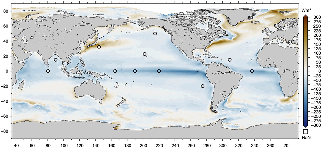
Figure 1. Long-term (30 years) average of global surface net heat flux obtained from J-OFURO3 V1.1 monthly data for 1988–2017. Positive values are upward heat flux. Unit in W m⁻². Locations of 11 buoys used in comparison are indicated as black circles.

TABLE 1

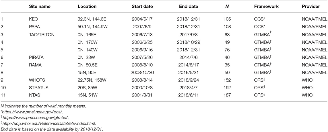
Table 1. Summary of buoy observation data used for the comparison with J-OFURO3.

The four surface heat flux components (SWR, LWR, LHF, and SHF) were calculated from the hourly observation data of each buoy. Subsequently, the daily average values were derived after the flux calculations. Furthermore, the monthly averaged value was calculated from the daily averaged value of the flux data. The NHF was calculated from the monthly average value, and if any components were missing, all the components were set as the missing values.

The flux calculation was performed according to the method described by Tomita et al. (2010). The net SWR was calculated from the observed downward SWR according to Equation (1):

$\begin{array}{ll}SWR=-\downarrow SWR(1-\alpha )& (1)\end{array}$

where α is the surface albedo, and the climatological monthly mean values on each grid obtained from the ISCCP have been used in this study. The net LWR was calculated from the observed downward LWR and the calculated upward LWR value from the sea surface temperature (SST) according to Equations (2) and (3),

$\begin{array}{ll}LWR=\uparrow LWR-\downarrow LWR& (2)\end{array}$

$\begin{array}{ll}\uparrow LWR=(\epsilon \sigma {SST}^4+(1-\epsilon )\downarrow LWR)& (3)\end{array}$

where ε is the emissivity at the ocean surface, set as 0.984 following Konda et al. (1994), and σ is the Stefan–Boltzmann constant (5.679 × 10⁻⁸ W m⁻² K⁻⁴).

For the LHF and SHF, the bulk flux calculation algorithm, COARE 3.0 (Fairall et al., 2003) was used. The input parameters required in the flux calculation using the algorithm are air temperature, humidity, winds, SST, and sea level pressure. For all parameters, the observed values at each buoy were used. The algorithm also requires the observation height of each parameter. The observation height information for each buoy listed in Supplementary Table 1 was used. For the SST, a skin/warm layer correction was not conducted.

The accuracy of the data on surface net heat flux obtained from in situ buoys is estimated to be 8 W/m² on average (Colbo and Weller, 2009; Cronin et al., 2019), while the values are slightly higher on a daily scale. For each flux component, the long-term averaged accuracy for SWR, LWR, LHF, and SHF are estimated 5.0, 3.9, 1.5, and 5.0 W/m², respectively. It can also be confirmed that the mid-latitude buoys (KEO) almost exhibit the same range (Tomita et al., 2010).

Comparison

The buoy data are point values while the satellite data are gridded. Therefore, we compared the values on gridded satellite data that include the locations of the buoys with the values calculated from the buoy measurements. All comparisons were conducted monthly. The statistics: bias, RMS, and correlation coefficient, r, were calculated for each flux component using the following equations:

$\begin{array}{l}bias=\frac{1}{n}{\displaystyle \sum _{l=1}^n}(s_l-b_l)\\ RMS=\sqrt{{\displaystyle \sum _{l=1}^n}\frac{{(s_l-b_l-bias)}^2}{n}}\\ r=\frac{{\displaystyle {\sum }_{l=1}^n}(s_l-\overline{s})(b_l-\overline{b})}{\sqrt{{\displaystyle {\sum }_{l=1}^n}{(s_l-\overline{s})}^2{\displaystyle {\sum }_{l=1}^n}{(b_l-\overline{b})}^2}}\end{array}$

where s and b are the satellite gridded value and buoy point value, respectively, and n is the number of monthly data at each buoy (see Table 1). It should be noted that the RMS is defined as a form in which the bias is removed from the difference between s and b (Taylor, 2001). All statistics values are available as Supplementary Data.

Results

Global Long-Term Mean

Figure 1 shows the distribution of the long-term (1988–2017) mean for the global NHF obtained from J3. The figure represents the climatological features of the distribution for the NHF. In the tropical zone, a net heat flux exists from the atmosphere to the ocean, and in mid- and high-latitudes, there is a net heat flux from the ocean to the atmosphere.

Examining regional features, there is a larger heat flux from the atmosphere to the ocean in the eastern tropical Pacific and at the equator. These areas contain upwelling ocean currents. In addition, there is large net heat flux from the ocean to the atmosphere at the western boundary current region for both hemispheres. Moreover, there is a strong flux contrast corresponding to the ocean fronts in these areas.

The global long-term average value calculated from J3 is −22.2 W m⁻². This indicates that the net heat flow is to the ocean surface. Although the characteristics of the qualitative distribution are not significantly different from common knowledge, this value is more than one order of magnitude larger from the viewpoint of global surface heat balance (NHF → 0).

The results are similar when compared with the global average value obtained from the previous generation dataset (J2). J2 data are only available for 1988–2008. The average values for J2 and J3 in 1988–2008 were 22.2 and 23.2 W m⁻², respectively.

Figure 2 shows the average values of the global NHF obtained by various estimation approaches. Except for the values of J2 and J3, the values are shown by Valdivieso et al. (2017). From this figure, with a few exceptions, the global long-term average of NHF tends to indicate a net heat flux to the ocean for most methodologies. Most satellite-based estimates, including J2 and J3, show greater ocean heating than those shown in ocean reanalysis estimates.

FIGURE 2

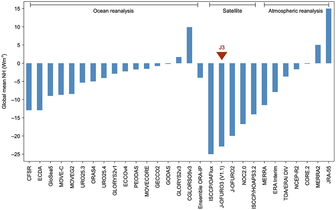
Figure 2. Comparison of global long-term averages among various estimates. The values (except for f J-OFURO2 and J-OFURO3) were drawn from Valdivieso et al. (2017). Positive values are upward heat flux. Almost all estimates are indicating ocean heating. Please also see the list of abbreviations of each dataset name and reference.

Figure 3 shows the balance among components that consist of NHF. In J3, the turbulent flux is smaller than the net radiation, resulting in an NHF of −22.2 W m⁻².

FIGURE 3

Figure 3. Balance of each component for the global long-term average of J-OFURO3 for the surface net heat flux (NHF). The balance for the turbulent heat flux (TUR) and the net surface radiation (RAD), in addition to the full components: the net shortwave radiation (SWR), the net long wave radiation (LWR), the latent heat flux (LHF), and the sensible heat flux (SHF) are shown.

Comparison With Buoys

Figure 4 shows the bias between the J3 estimates and buoy observations. At all buoy points except RAMA (15N, 90E), the bias is negative, indicating a significant ocean heating bias in J3. In particular, large negative biases were found in buoys in the western tropical Pacific (0N, 165E), central tropical Pacific (0N, 170W), and central tropical Indian Ocean (0N, 80.5E). The overall averaged bias is −5.8 W m⁻², and the averaged bias at mid-high latitudes excluding buoys in the tropical zone is −3.1 W m⁻², which shows good agreement.

FIGURE 4

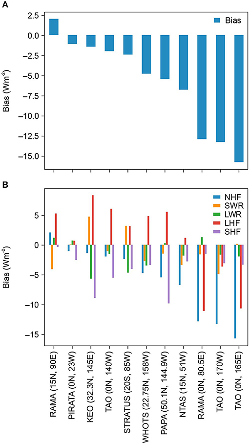
Figure 4. Biases (J-OFURO3 minus buoys) of the surface heat fluxes at each buoy site for (A) the surface net heat flux (NHF) and (B) components. The comparison results are based on 1,063 monthly means from 11 sites.

There are cases in which the positive and negative biases of each component cancel each other out (Figure 4B). For example, at KEO, SW, and LH show positive biases, while LW and SH show negative biases. The sum of absolute biases of the components is 27.6 W m⁻², which is significantly larger than the absolute NHF bias of 1.5 W m⁻². Similar canceling out of biases was seen in Stratus, RAMA (15N, 90E), and TAO (0N, 140W).

Unexpectedly, Figure 4B indicates that the SH bias is always negative for these data, while biases of the other components show both negative and positive biases depending on the buoy locations. A comparison using more comprehensive global buoy data that can calculate turbulent heat flux confirms these negative SH biases, especially over the open ocean area (Tomita et al., 2019). The influence of SH biases on the global long-term mean of NHF is discussed in the “Discussion” section.

In addition, a pattern of characteristic bias was also observed in the LW. Relatively large negative biases in LW were found in the KEO, STRATUS, and WHOTS buoys located in the subtropics and mid-latitudes. The negative LW biases were relatively small at buoys in the tropics. The KEO and STRATUS buoy networks correspond to areas that have significant cloudiness consisting of low-level clouds.

The same comparisons were made using both J2 and J3 data for the period up to 2008. An improvement from the previous generation data was confirmed. Figure 5 shows the bias, RMS, and the correlation for the NHF for J2 and J3. From the data in this figure, significant improvements in statistics from J2 were confirmed. At most buoy points, the RMS and correlation coefficients are improved. For the bias, on average, the absolute bias of J3 is slightly higher than that of J2. However, J2 has a small bias due to canceling out of the large positive and large negative biases. Such large positive and negative biases were improved in J3, while a slight negative bias was observed.

FIGURE 5

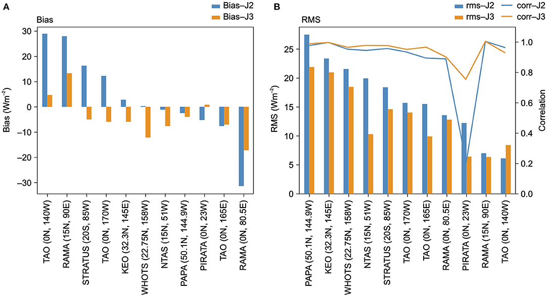
Figure 5. Advances in comparative statistics of the (A) bias, (B) RMS, and correlation coefficient of surface net heat flux (NHF) for J-OFURO2 (J2) and J-OFURO3 V1.1 (J3). Note that the buoys are listed in different orders in (A) and (B).

Consistency With Freshwater Flux

The LHF, which is one of the surface heat flux components, is proportional to the evaporation rate from the ocean surface and is a part of the freshwater flux as a counterpart for precipitation. Therefore, by checking the consistency between the latent heat flux (evaporation) and the surface freshwater balance one can evaluate the surface heat balance from a different perspective.

In general, the global ocean freshwater flux defined as (evaporation minus precipitation) is positive because a significant amount of water evaporates from the ocean. The evaporated water is transported to land by atmospheric advection, mainly in the form of water vapor. On a long-term average, the changes in atmosphere disappear and the net positive freshwater flux over the ocean is balanced by the runoff of river water from the continent into the ocean (i.e., freshwater flux–runoff = 0).

The global long-term mean value of ocean evaporation in J3 was 3.4 mm/day, while the precipitation over the ocean obtained from GPCP V2.3 was 3.0 mm/day. Therefore, the global long-term mean of freshwater flux was calculated as 0.4 mm per day. The result showed a good balance after considering the runoff from land. Various estimates have been obtained by studies on river runoff. These values range from approximately 0.27 to 0.34 mm/day (Schlosser and Houser, 2007). More recent studies estimate river runoff as 0.29 (Ghiggi et al., 2019) and 0.31 (Wilkinson et al., 2014) mm/day. According to these previous studies, if we assume a value of 0.3 mm/day of river runoff, the freshwater balance estimated from J3, GPCP, and the river runoff is 0.1 mm/day, which is a reasonable result. An improvement was confirmed compared to the estimation using J-OFURO2 (Iwasaki et al., 2014).

Although there are various global precipitation datasets (Kidd and Huffman, 2011), GPCP is used as the standard dataset in numerous studies (e.g., Andersson et al., 2011; Tapiador et al., 2017; Yu, 2019; Gutenstein et al., 2021). However, most studies suggest that much of the uncertainty in water balance lies in precipitation products as well as evaporation. To confirm the differences in the results that depend on the satellite products, we reconfirmed the results using another satellite precipitation/evaporation product, HOAPS-4.0. Consequently, it was confirmed that the long-term mean precipitation of HOAPS-4.0 for 1988–2014 (2.9 mm/day) was slightly smaller than that of GPCP V2.3 for the same period (3.0 mm/day). For evaporation, the long-term mean HOAPS-4.0 value for 1988–2014 was 3.4 mm/day. Therefore, the global ocean freshwater flux value (0.5 mm/day) was slightly higher than that estimated by J3 (0.4 mm/day, for 1988–2014), while being sufficiently comparable.

Discussion

The global long-term mean value of the NHF from the J3 data was consistent with the previous generation data. The tendency of ocean heating is similar to other estimates such as satellite and ocean reanalysis. However, its value was large in magnitude, −22.2 W m⁻², indicating a significant negative imbalance. In contrast, by comparison with local 11 buoys, the average bias was found to be −5.8 W m⁻² and the negative largest value of −15.7 W m⁻² was found at buoy in the western tropical Pacific. Therefore, the relationship between the global mean value of J3 and the local bias was inconsistent, and the paradox of surface heat flux was confirmed. In previous studies (Pinker et al., 2017; Valdivieso et al., 2017), several tropical and subtropical buoys data (Stratus) were used for the evaluation of surface net heat flux. In contrast, for this study, the comparison was performed using more buoy data which included mid-high latitude buoys (KEO and PAPA). These data contained longer time series, and the paradox was confirmed. The cause is discussed in the following text.

In contrast to the excessively large negative imbalance for the NHF in the global long-term mean, the globally averaged ocean surface freshwater flux estimated by surface latent heat flux (evaporation) in J3, GPCP, and runoff was almost 0. This result was consistent with a previous estimate (Trenberth et al., 2007). Because the sum of these independently estimated components was close to 0, J3 the LHF is considered to be very reliable. Therefore, the cause of the imbalance might be other than the LHF. The comparison of the J3 LHF with more comprehensive global buoys (Figure 6A) revealed that the total bias was fairly small (<1 W m⁻²) while there are some regional biases. This fact also strongly suggests that the cause of the excessively large global long-term mean imbalance of NHF is likely to be other than LHF.

FIGURE 6

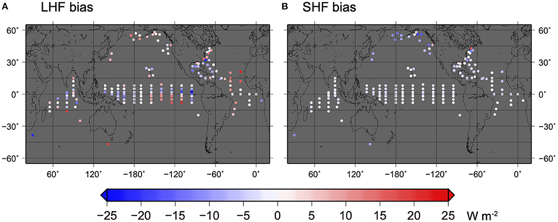
Figure 6. Biases (J-OFURO3 V1.1 minus buoy) of (A) latent heat flux (LHF) and (B) sensible heat flux (SHF). The biases in this figure were calculated from global buoy data used in the J-OFURO3 Quality Check System (Tomita and Hihara, 2017).

In contrast to the LHF, the J3 SHF had a persistent bias. As shown in the Results (Section “Comparison with Buoys”), the SHF showed negative biases in the comparisons with all of the 11 buoys. Negative biases were also confirmed by comparison with more comprehensive buoy observations (Figure 6B). There are negative biases in almost all open ocean areas except for the coastal area, and a larger negative bias occurs especially in mid-high latitudes (Tomita et al., 2019). Figure 7 shows the bias of the SHF as a function of latitude. In order to investigate the effect of this SHF bias characteristic on the global averaged value, this bias was corrected by using a fitting curve and the global averaged value was recalculated. The global long-term mean value of the SHF without bias correction was +8.1 W m⁻², while the global long-term average value after bias correction was 13.3 W m⁻². This bias correction has an impact of improving the global mean of the NHF by +5.5 W m⁻², but a large imbalance of −16.7 W m⁻² still remains. However, the number of buoy observations on which this bias correction was based does not completely cover global oceans (as seen in Figure 6B). It is necessary to consider a more robust correction method in the future. As shown in Figure 7B, the cause of this SHF bias is in the air temperature. The J3 uses atmospheric reanalysis data instead of satellite retrieval for air temperature estimation, and it is desirable to refer to better air temperature estimates or develop a satellite-based retrieval method in the future.

FIGURE 7

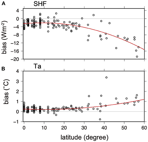
Figure 7. Biases (J-OFURO3 V1.1 minus buoy) of (A) surface sensible heat flux (SHF) and (B) air temperature (Ta) as a function of latitudes. The solid lines show 2nd order polynormal fitting curves. The biases in this figure were calculated from global buoy data used in the J-OFURO3 Quality Check System (Tomita and Hihara, 2017). Note that the data in near coastal region (the distance from coastline <200 km) were removed in this comparison.

Furthermore, the data coverage of J3 SHF over high-latitudes is small. In the presence of sea ice, J3 cannot calculate the turbulent heat flux; therefore, the estimation of turbulent heat flux over regions with sea ice is overlooked. In a simple test performed using ERA5 (Hersbach et al., 2020), which has complete global coverage, the global ocean average value is approximately 30% smaller than the original ERA5 value when the sea ice area is excluded for simulating the coverage of J3. When including the sea ice region, the global ocean average SHF value is approximately 1.4 times larger. This is a reasonable result considering the large air–sea temperature difference (i.e., large SHF) with sea ice at high latitudes. The same test for LHF does not give the same result. In the case of LHF, the value corresponding to the sea ice region does not have a large influence on the global ocean averages, and by including the sea ice region, the global averaged value decreases slightly. In addition to the bias correction mentioned above, when assuming that the global ocean average of J3 SHF is approximately 1.4 times larger, the NHF value changes to the improved value (−11.3 W/m²), which is approximately half the original value (−22.2 W/m²). This indicates the limits of microwave satellite-based flux products such as J3 and the importance of considering the value of SHF over the sea ice region in the global ocean heat balance.

The LWR also had a notable bias characteristic. The LWR bias was relatively small in the tropics, while it was comparatively large in the subtropics and mid-latitudes. For example, the largest biases were found in the KEO and Stratus data. These were −5.7 and −4.7 W m⁻², respectively. A detailed comparison was performed to investigate the cause in detail. Figure 8 shows the bias in the upward and downward components of the long wave radiation described by Equation (2). As shown in Equation (3), the upward component of the LWR is not completely independent of the downward component, but the bias shows small negative values (<1 W m⁻²). The major factor of the LWR bias is the downward component. Validation of the downward LWR assessments was performed using more comprehensive buoy observations (Rutan et al., 2015; Kato et al., 2018). Our results are consistent with their results, indicating that the bias is <5 W m⁻²; however, the spatial characteristics of the error have never been investigated thoroughly.

FIGURE 8

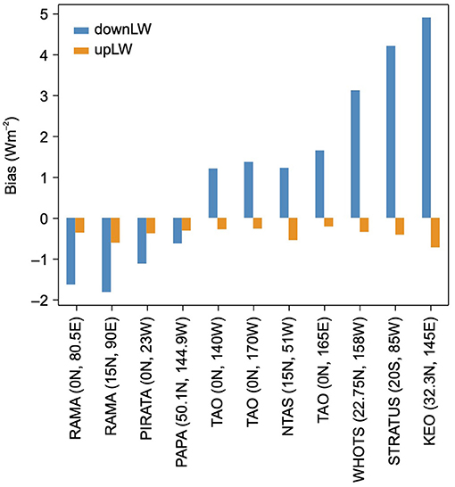
Figure 8. Biases (J-OFURO3 minus buoy) of downward and upward components of the long wave radiations.

The buoy locations of Stratus and KEO are known as oceanic areas frequently covered by low-level clouds (e.g., Klein and Hartmann, 1993). In contrast, for the high latitude area of the North Pacific, PAPA, which is also characterized by low-level clouds, the downward LWR shows a good agreement. A more detailed investigation of the bias and the relationship with clouds, air temperature, and sea surface temperature will be needed better understand this phenomenon.

In the above, we discussed the possibility of large biases outside the 11 buoys (which showed relatively good agreement on the global heat balance). As another possibility, we discuss the effect of the difference due to the bulk formula and the associated calculation method on the global heat balance. In general, the selection of a bulk formula has a major influence on the estimation of the global turbulent heat and momentum fluxes. Based on a comparative study (Brunke et al., 2003; Iwasaki et al., 2010), COARE 3.0 is used in J3 and other satellite products. Brodeau et al. (2017) estimated that changes in the bulk formula will affect the global heat balance by 10%, and the use of different bulk formulae may significantly change the global heat balance. However, it is necessary to pay attention to consistency with other physics by changing the bulk formula. Yu (2019) confirmed that although the global heat balance was improved by changing the bulk formula, the change in LH caused a freshwater imbalance. Similar results are expected for J3. Improvements in the bulk formula for turbulent heat fluxes are needed, while maintaining consistency with other physics.

In this study, we focused on the long-term mean surface net heat flux. The daily satellite-derived data set is very useful for analyzing the flux variation over time-scales varying from several days to inter-annual or decades. This type of analysis was not in the scope of this research. Weller (2015) showed that precise and long-term buoy observation revealed long-term flux trends. It will be useful for the verification of satellite data in the future. However, the number of buoys will still be small to understand the overall characteristics of these fluctuations.

In general, the uncertainty of precipitation and evaporation from the ocean is a major challenge in understanding of the water cycle. Improving satellite-based products should address this challenge. In this study, the state-of-the-art satellite-based products, J-OFURO3 (Tomita et al., 2019) and HOAPS-4.0 (Andersson et al., 2017), were confirmed to be consistent with each other in the estimation of freshwater flux, which confirms the improvement of satellite products. Estimating and providing uncertainty information is also important. An approach that combines satellite and ocean observations with the estimation of atmospheric energy transport derived from atmospheric reanalysis data is also a powerful tool to better estimate global surface fluxes (e.g., Liu et al., 2015, 2017; Carton et al., 2018). In the future, it will be necessary to combine multiple approaches, while improving satellite products by their comparison with such approaches.

Data Availability Statement

Publicly available datasets were analyzed in this study. This data can be found here: The J-OFURO3 V1.1 dataset analyzed for this study can be found in the DIAS, and APDRC (https://doi.org/10.20783/DIAS.612); the GPCP precipitation data for this study can be found at https://psl.noaa.gov/data/gridded/data.gpcp.html; the satellite-derived surface radiation data for this study can be found at CERES: https://ceres.larc.nasa.gov/data/ and ISCCP: https://isccp.giss.nasa.gov/products/onlineData.html; the HOAPS data for this study can be found at https://wui.cmsaf.eu/safira/action/viewDoiDetails?acronym=HOAPS_V002; and the surface moored buoy data for this study can be found at NOAA PMEL: https://www.pmel.noaa.gov/ocs/, https://www.pmel.noaa.gov/gtmba/ and WHOI: http://uop.whoi.edu/ReferenceDataSets/index.html.

Author Contributions

HT designed the study, led the research, interpreted the data, wrote the manuscript, and managed the project. HT analyzed global satellite-based surface heat flux datasets. KK, TH, and HT collected in situ buoy observation data and calculated surface heat fluxes. KK and HT compared satellite estimates with buoy observations. TH contributed some useful scripts for this study. All authors contributed to improving the manuscript.

Funding

This work was supported by JSPS KAKENHI Grant Numbers JP18H03726, JP26287114, JP18H03737, and JP19H05696. The Japan Aerospace Exploration Agency (JAXA), Institute for Space-Earth Environmental Research of Nagoya University, and the Institute of Oceanic Research and Development of Tokai University (Grants # 2018–5 and 2019–5) also partly support this research.

Conflict of Interest

The authors declare that the research was conducted in the absence of any commercial or financial relationships that could be construed as a potential conflict of interest.

Acknowledgments

GPCP precipitation data provided by the NOAA/OAR/ESRL PSL, Boulder, Colorado, USA, from their website at https://psl.noaa.gov/. Satellite-derived surface radiation data were provided by the projects NASA CERES and ISCCP. HOAPS data provided by EUMETSAT CM SAF. Surface moored buoy data were provided by NOAA PMEL and WHOI.

Supplementary Material

The Supplementary Material for this article can be found online at: https://www.frontiersin.org/articles/10.3389/fmars.2021.612361/full#supplementary-material

Abbreviations

AMI, Active Microwave Instrument; AMSR-E, Advanced Microwave Scanning Radiometer—Earth observing system; ASCAT, Advanced Scatterometer; CFSR, NCEP Climate Forecast System Reanalysis (Xue et al., 2011); CGLORS 05V3, Ocean reanalysis at the Centro Euro-Mediterraneo sui Cambiamenti Climatici (CMCC) (Storto et al., 2014); CORE.2, Common Ocean Reference Experiment Version 2, known as the flux product of Large and Yeager (2009); ECCO v4, The Estimating the Circulation and Climate of the Ocean (https://www.ecco-group.org); ECDA, Ensemble Coupled Data Assimilation; ERA Interim, European Center for Medium-Range Weather Forecasts Reanalysis-Interim (Dee et al., 2011); ERA5, European Center for Medium-Range Weather Forecasts Reanalysis-5 (Hersbach et al., 2020); ERS, European Space Agency (ESA) Remote-Sensing Satellite; GECCO2, The German contribution of the Estimating the Circulation and Climate of the Ocean project (ECCO); GLORYS2 v1 and v3, Ocean reanalysis at Mercator Ocean: https://www.mercator-ocean.fr/en/science-publications/glorys/; GloSea5, UK Met Office Global Seasonal Forecasting System version 5 (Scaife et al., 2014; MacLachlan et al., 2015); GODAS, NCEP Global Ocean Data Assimilation System; HOAPS, Hamburg Ocean Atmosphere Parameters and Fluxes from Satellite data (Andersson et al., 2011, 2017); ISCCP, International Satellite Cloud Climatology Project; J-OFURO, Japanese Ocean Flux Data Sets with Use of Remote Sensing Observations (Tomita et al., 2019); JRA-55, the Japanese 55-year Reanalysis (Kobayashi et al., 2015); MERRA, Modern-Era Retrospective analysis for Research and Applications; MOVE-C, Multivariate Ocean Variational Estimation System–Coupled Version Reanalysis; NCEP-R2, NCEP-DOE AMIP-II reanalysis (Kanamitsu et al., 2002); NOC, National Oceanography Center; OAFlux, Objectively Analyzed Air-sea Fluxes (Yu and Weller, 2007); ORA-IP, Ocean Reanalysis Intercomparison Project (Balmaseda et al., 2015); ORAS4, ECMWF operational ocean reanalysis (Balmaseda et al., 2013); OSCAT, Oceansat-2 Scatterometer; PEODAS, Predictive Ocean Atmosphere Model for Australia (POAMA) Ensemble Ocean Data Assimilation System (Yin et al., 2011); SSMI, Special Sensor Microwave Imager; SSMIS, Special Sensor Microwave Imager/Sounder; TMI, Tropical Rainfall Measurement Mission (TRMM) Microwave Imager; TOA CERES/ERAi DIV, The hybrid product of CERES and ERA-Interim (Liu et al., 2015); UR025.3 and 025.4, University of Reading global ocean reanalysis.

References

Adler, R. F., Huffman, G. J., Chang, A., Ferraro, R., Xie, P., Janowiak, J., et al. (2003). The version 2 global precipitation climatology project (GPCP) monthly precipitation analysis (1979-present). J. Hydrometeor. 4,1147–1167. doi: 10.1175/1525-7541(2003)004<1147:TVGPCP>2.0.CO;2

CrossRef Full Text | Google Scholar

Andersson, A., Graw, K., Schroder, M., Fennig, K., Liman, J., Bakan, S., et al. (2017). Hamburg Ocean Atmosphere Parameters and Fluxes from Satellite Data—HOAPS 4.0, Satellite Application Facility on Climate Monitoring, Data set. doi: 10.5676/EUM_SAF_CM/HOAPS/V002

CrossRef Full Text | Google Scholar

Andersson, A., Klepp, C., Fennig, K., Bakan, S., Grassl, H., and Schulz, J. (2011). Evaluation of HOAPS-3 ocean surface freshwater flux components. J. Appl. Meterol. Climatol. 50, 379–398. doi: 10.1175/2010JAMC2341.1

CrossRef Full Text | Google Scholar

Balmaseda, M. A., Hernandez, F., Storto, A., Palmer, M. D., Alves, O., Shi, L., et al. (2015). The ocean reanalyses intercomparison project (ORA-IP). J. Oper. Oceanogr. 8, s80–s97. doi: 10.1080/1755876X.2015.1022329

CrossRef Full Text | Google Scholar

Balmaseda, M. A., Mogensen, K., and Weaver, A. T. (2013). Evaluation of the ECMWF ocean reanalysis system ORAS4. Quart. J. R. Meterol. Soc. 139, 1132–1161. doi: 10.1002/qj.2063

CrossRef Full Text | Google Scholar

Bentamy, A., Piollé, J. F., Grouazel, A., Danielson, R., Gulev, S., and Paul, F. (2017). Review and assessment of latent and sensible heat flux accuracy over the global oceans. Remote Sens. Environ. 201,196–218. doi: 10.1016/j.rse.2017.08.016

CrossRef Full Text | Google Scholar

Brodeau, L., Barnier, B., Gulev, S. K., and Woods, C. (2017). Climatologically significant effects of some approximations in the bulk parameterizations of turbulent air–sea fluxes. J. Phys. Oceanogr. 47, 5–28. doi: 10.1175/JPO-D-16-0169.1

CrossRef Full Text | Google Scholar

Brunke, M. A., Fairall, C. W., Zeng, X., Eymard, L., and Curry, J. A. (2003). Which bulk aerodynamic algorithms are least problematic in computing ocean surface turbulent fluxes? J. Clim. 16, 619–635. doi: 10.1175/1520-0442(2003)016<0619:WBAAAL>2.0.CO;2

CrossRef Full Text | Google Scholar

Carton, J. A., Chepurin, G. A., Chen, L., and Grodsky, S. A. (2018). Improved global net surface heat flux. J. Geophys. Res. Oceans 123, 3144–3163. doi: 10.1002/2017JC013137

CrossRef Full Text | Google Scholar

Colbo, K., and Weller, R. A. (2009). Accuracy of the IMET sensor package in the subtropics. J. Atmos. Ocean. Technol. 26, 1867–1890. doi: 10.1175/2009JTECHO667.1

CrossRef Full Text | Google Scholar

Cronin, M. G., Gentemann, C. L., Edson, J., Ueki, I., Bourassa, M., Brown, S., et al. (2019). Air-sea fluxes with a focus on heat and momentum. Front. Mar. Sci 6:430. doi: 10.3389/fmars.2019.00430

CrossRef Full Text | Google Scholar

Dee, D. P., Uppala, S. M., Simmons, A. J., Berrisford, P., Poli, P., Kobayashi, P. S., et al. (2011). The ERA-Interim reanalysis: configuration and performance of the data assimilation system. Quart. J. R. Meterol. Soc. 137, 553–597. doi: 10.1002/qj.828

CrossRef Full Text | Google Scholar

Doelling, D. R., Loeb, N. G., Keyes, D. F., Nordeen, M. L., Morstad, D., Nguyen, C., et al. (2013). Geostationary enhanced temporal interpolation for CERES flux products. J. Atmos. Ocean. Technol. 30, 1072–1090. doi: 10.1175/JTECH-D-12-00136.1

CrossRef Full Text | Google Scholar

Doelling, D. R., Sun, M., Nguyen, L. T., Nordeen, M. L., Haney, C. O., Keyes, D. F., et al. (2016). Advances in geostationary-derived longwave fluxes for the CERES Synoptic (SYN1deg) product. J. Atmos. Ocean. Technol. 33, 503–521. doi: 10.1175/JTECH-D-15-0147.1

CrossRef Full Text | Google Scholar

Fairall, C. W., Bradley, E. F., Hare, J. E., Grachev, A. A., and Edson, J. B. (2003). Bulk parameterization of air-sea fluxes: updates and verification for the COARE algorithm. J. Clim. 16, 571–591.

Google Scholar

Ghiggi, G., Humphrey, V., Seneviratne, S. I., and Gudmundsson, L. (2019). GRUN: an observation-based global gridded runoff dataset from 1902 to 2014. Earth Syst. Sci. Data 11, 1655–1674, doi: 10.5194/essd-11-1655-2019

CrossRef Full Text | Google Scholar

Gutenstein, M., Fennig, K., Schröder, M., Trent, T., Bakan, S., Roberts, J. B., et al. (2021). Intercomparison of freshwater fluxes over ocean and investigations into water budget closure. Hydrol. Earth Syst. Sci. 25, 121–146. doi: 10.5194/hess-2020-317

CrossRef Full Text | Google Scholar

Hersbach, H., Bell, B., Berrisford, P., Hirahara, S., Horányi, A., Muñoz-Sabater, J., et al. (2020). The ERA5 global reanalysis. Quart. J. R. Meterol. Soc. 146, 1999–2049. doi: 10.1002/qj.3803

CrossRef Full Text | Google Scholar

Iwasaki, S., Kubota, M., and Tomita, H. (2010). Evaluation of bulk method for satellite-derived latent heat flux. J. Geophys. Res. 115:C07007. doi: 10.1029/2010JC006175

CrossRef Full Text | Google Scholar

Iwasaki, S., Kubota, M., and Watabe, T. (2014). Assessment of various global freshwater flux products for the global ice-free oceans. Remote Sens. Environ. 140, 549–561. doi: 10.1016/j.rse.2013.09.026

CrossRef Full Text | Google Scholar

Kanamitsu, M., Ebitsuzaki, W., Woolen, J., Yang, S. K., Hnilo, J. J., Fiorino, M., et al. (2002). NCEP-DOE AMIP-II reanalysis (R-2). Bull. Am. Meterol. Soc. 83, 1631–1643. doi: 10.1175/BAMS-83-11-1631(2002)083<1631:NAR>2.3.CO;2

CrossRef Full Text | Google Scholar

Kato, S., Rose, F. G., Rutan, D. A., Thorsen, T. J., Loeb, N. G., Doelling, D. R., et al. (2018). Surface irradiances of Edition 4.0 clouds and the earth's radiant energy system (CERES) energy balanced and filled (EBAF) data product. J. Clim. 31, 4501–4527. doi: 10.1175/JCLI-D-17-0523.1

CrossRef Full Text | Google Scholar

Kidd, C., and Huffman, G. (2011). Global precipitation measurement. Meterol. Appl. 18, 334–353. doi: 10.1002/met.284

CrossRef Full Text | Google Scholar

Klein, S. A., and Hartmann, D. L. (1993). The seasonal cycle of low stratiform clouds. J. Clim. 6, 1587–1606. doi: 10.1175/1520-0442(1993)006<1587:TSCOLS>2.0.CO;2

CrossRef Full Text | Google Scholar

Kobayashi, S., Ota, Y., Harada, Y., Ebita, A., Moriya, M., Onoda, H., et al. (2015). The JRA-55 reanalysis: general specifications and basic characteristics. J. Meterol. Soc. Jpn. 93, 5–48. doi: 10.2151/jmsj.2015-001

CrossRef Full Text | Google Scholar

Konda, M., Imasato, N., Nishi, K., and Toda, T. (1994). Measurement of the sea surface emissivity. J. Oceanogr. 50, 17–30. doi: 10.1007/BF02233853

CrossRef Full Text | Google Scholar

Kubota, M., Iwasaka, N., Kizu, S., Konda, M., and Kutsuwada, K. (2002). Japanese ocean flux data sets with use of remote sensing observations (J-OFURO). J. Oceanogr. 58, 213–225. doi: 10.1023/A:1015845321836

CrossRef Full Text | Google Scholar

Large, W. G., and Yeager, S. G. (2009). The global climatology of an interannually varying air–sea flux data set. Clim. Dyn. 33, 341–364. doi: 10.1007/s00382-008-0441-3

CrossRef Full Text | Google Scholar

Liu, C., Allan, R. P., Berrisford, P., Mayer, M., Hyder, P., Loeb, N., et al. (2015). Combining satellite observations and reanalysis energy transports to estimate global net surface energy fluxes 1985–2012. J. Geophys. Res. Atmos.120, 9374–9389. doi: 10.1002/2015JD023264

CrossRef Full Text | Google Scholar

Liu, C., Allan, R. P., Berrisford, P., Mayer, M., Hyder, P., Loeb, N., et al. (2017). Evaluation of satellite and reanalysis-based global net surface energy flux and uncertainty estimates. J. Geophys. Res. Atmos. 122, 6250–6272. doi: 10.1002/2017JD026616

PubMed Abstract | CrossRef Full Text | Google Scholar

Loeb, N. G., Su, W., Doelling, D. R., Wong, T., Minnis, P., Thomas, S., et al. (2018). Earth's top-of-atmosphere radiation budget. Compr. Remote Sen. 5, 67–84. doi: 10.1016/B978-0-12-409548-9.10367-7

CrossRef Full Text | Google Scholar

MacLachlan, C., Arribas, A., Peterson, K. A., Maidens, A., Fereday, D. A., Scaife, A., et al. (2015). Description of GloSea5: the Met Office high resolution seasonal forecast system. Quart. J. R. Meterol. Soc. 141, 1072–1084. doi: 10.1002/qj.2396

CrossRef Full Text | Google Scholar

McPhaden, M., Busalacchi, A., Cheney, R., Donguy, J.-R., Gage, K., Halpern, D., et al. (1998). The tropical ocean global atmosphere observing system: a decade of progress. J. Geophys. Res. 103:14169–14240. doi: 10.1029/97JC02906

CrossRef Full Text | Google Scholar

McPhaden, M. J., Meyers, G., Ando, K., Masumoto, Y., Murty, V. S. N., Ravichandran, M., et al. (2009). RAMA: the research moored array for African–Asian–Australian monsoon analysis and prediction. Bull. Am. Meterol. Soc. 90, 459–480. doi: 10.1175/2008BAMS2608.1

CrossRef Full Text | Google Scholar

Pinker, R. T., Bentamy, A., Katsaros, K. B., Ma, Y., and Li, C. (2014). Estimates of net heat fluxes over the Atlantic Ocean. J. Geophys. Res. Oceans 119, 410–427. doi: 10.1002/2013JC009386

CrossRef Full Text | Google Scholar

Pinker, R. T., Bentamy, A., Zhang, B., Chen, W., and Ma, Y. (2017). The net energy budget at the ocean-atmosphere interface of the “Cold Tongue” region. J. Geophys. Res. Oceans 122, 5502–5521. doi: 10.1002/2016JC012581

CrossRef Full Text | Google Scholar

Rossow, W. B., and Schiffer, R. A. (1991). ISCCP cloud data products. Bull. Am. Meterol. Soc. 71, 2–20. doi: 10.1175/1520-0477(1991)072<0002:ICDP>2.0.CO;2

CrossRef Full Text | Google Scholar

Rutan, D. A., Kato, S., Doelling, D. R., Rose, F. G., Nguyen, L. T., Caldwell, T. E., et al. (2015). CERES Synoptic product: methodology and validation of surface radiant flux. J. Atmos. Oceanic Technol. 32, 1121–1143. doi: 10.1175/JTECH-D-14-00165.1

CrossRef Full Text | Google Scholar

Scaife, A. A., Arribas, A., Blockley, E., Brookshaw, A., Clark, R. T., Dunstone, N., et al. (2014). Skilful long range prediction of European and North American winters. Geophys. Res. Lett. 41, 2514–2519. doi: 10.1002/2014GL059637

CrossRef Full Text | Google Scholar

Schlosser, C. A., and Houser, P. R. (2007). Assessing a satellite-era perspective of the global water cycle. Clim. J. 20, 1316–1338. doi: 10.1175/JCLI4057.1

CrossRef Full Text | Google Scholar

Schulz, E. W., Josey, S. A., and Verein, R. (2012). First air-sea flux mooring measurements in the Southern Ocean. Geophys. Res. Lett. 39:L16606. doi: 10.1029/2012GL052290

CrossRef Full Text | Google Scholar

Servain, J., Busalacchi, A. J., McPhaden, M. J., Moura, A. D., Reverdin, G., Vianna, M., et al. (1998). A pilot research moored array in the Tropical Atlantic (PIRATA). Bull. Am. Meterol Soc. 79, 2019–2031. doi: 10.1175/1520-0477(1998)079<2019:APRMAI>2.0.CO;2

CrossRef Full Text | Google Scholar

Storto, A., Masina, S., and Dobricic, S. (2014). Estimation and impact of nonuniform horizontal correlation length scales for global ocean physical analyses. J. Atmos. Ocean. Technol. 31, 2330–2349. doi: 10.1175/JTECH-D-14-00042.1

CrossRef Full Text | Google Scholar

Tapiador, F. J., Navarro, A., Levizzani, V., García-Ortega, E., Huffman, G. J., Kidd, C., et al. (2017). Global precipitation measurements for validating climate models. Atmos. Res.197, 1–20. doi: 10.1016/j.atmosres.2017.06.021

CrossRef Full Text | Google Scholar

Taylor, K. E. (2001). Summarizing multiple aspects of model performance in a single diagram. J. Geophys. Res. Atmos. 106, 7183–7192. doi: 10.1029/2000JD900719

CrossRef Full Text | Google Scholar

Tomita, H. (2017). J-OFURO3 data set detailed document, J-OFURO3 official document, J-OFURO3_DOC_002 (V1.1E). doi: 10.18999/27183

CrossRef Full Text | Google Scholar

Tomita, H., and Hihara, T. (2017). Quality check system for J-OFURO3, J-OFURO3 official document, J-OFURO3_DOC_006, V1.0E. doi: 10.18999/27211

CrossRef Full Text | Google Scholar

Tomita, H., Hihara, T., Kako, S., Kubota, M., and Kutsuwada, K. (2019). An introduction to J-OFURO3, a third-generation Japanese ocean flux data set using remote-sensing observations. J. Oceanogr. 75, 171–194. doi: 10.1007/s10872-018-0493-x

CrossRef Full Text | Google Scholar

Tomita, H., Hihara, T., and Kubota, M. (2018). Improved satellite estimation of near-surface humidity using vertical water vapor profile information. Geophys. Res. Lett. 45, 899–906. doi: 10.1002/2017GL076384

CrossRef Full Text | Google Scholar

Tomita, H., Kubota, M., Cronin, M. F., Iwasaki, S., Konda, M., and Ichikawa, H. (2010). An assessment of surface heat fluxes from J-OFURO2 at the KEO and JKEO sites. J. Geophys. Res. 115:C03018. doi: 10.1029/2009JC005545

CrossRef Full Text | Google Scholar

Trenberth, K. E., Smith, L., Qian, T., Dai, A., and Fasullo, J. (2007). Estimates of the global water budget and its annual cycle using observational and model data. J. Hydrometeor. 8, 758–769. doi: 10.1175/JHM600.1

CrossRef Full Text | Google Scholar

Valdivieso, M., Haines, K., Balmaseda, M., Chang, Y.-S., Drevillon, M., Ferry, N., et al. (2017). An assessment of air–sea heat fluxes from ocean and coupled reanalyses. Clim. Dyn. 49, 983–1008. doi: 10.1007/s00382-015-2843-3

CrossRef Full Text | Google Scholar

Weller, R. A. (2015): Variability and trends in surface meteorology and air–sea fluxes at a site off Northern Chile. Clim. J. 28, 3004–3023. doi: 10.1175/JCLI-D-14-00591.1

CrossRef Full Text | Google Scholar

Wilkinson, K., von Zabern, M., and Scherzer, S. (2014). Global Freshwater Fluxes Into the World Oceans. GRDC Report Series, UDATA Umweltschutz und Datenanalyse, Neustadt, 44, 9pp.

Xue, Y., Huang, B., Hu, Z.-Z., Kumar, A., Wen, C., Behringer, D., and Nadiga, S. (2011). An assessment of oceanic variability in the NCEP climate forecast system reanalysis. Clim Dyn. 37, 2511–2539. doi: 10.1007/s00382-010-0954-4

CrossRef Full Text | Google Scholar

Yin, Y., Alves, O., and Oke, P. (2011). An ensemble ocean data assimilation system for seasonal prediction. Mon. Weather Rev. 139, 786–808. doi: 10.1175/2010MWR3419.1

CrossRef Full Text | Google Scholar

Yu, L. (2019). Global air–sea fluxes of heat, fresh water, and momentum: energy budget closure and unanswered questions. Annu. Rev. Mar. Sci. 11, 227–248. doi: 10.1146/annurev-marine-010816-060704

PubMed Abstract | CrossRef Full Text | Google Scholar

Yu, L., and Weller, R. A. (2007). Objectively analyzed air–sea heat fluxes for the global ice-free oceans (1981–2005). Bull. Am. Meterol. Soc. 88, 527–540. doi: 10.1175/BAMS-88-4-527

CrossRef Full Text | Google Scholar