A Fuzzy-Based Framework for Assessing Uncertainty in Drift Prediction Using Observed Currents and Winds

1. Introduction

The ability to respond to emergencies such as marine contaminant spills and search and rescue efforts is directly linked with the ability to predict the trajectories of objects drifting at the ocean surface (Daniel et al., 2002; Breivik and Allen, 2008; Davidson et al., 2009; Butler, 2015). Better predictions of trajectories also enhance our understanding of marine ecosystem functioning and connectivity (Checkley et al., 1988; Gawarkiewicz et al., 2007; Röhrs et al., 2014; Stark et al., 2018). Drift trajectories of floating objects are governed by currents and winds at the very surface of the ocean. These remain persistently difficult to measure (Soloviev and Lukas, 2014), and the submesoscale variability of these fields can only be measured directly during targeted campaigns of limited duration (Poje et al., 2014; D'Asaro et al., 2018). Therefore, further treatment is generally required to properly characterize uncertainty arising from imprecise measurements of surface currents and winds. In practice, currents and winds used to force drift trajectory simulations are usually obtained from numerical circulation models, which introduces further uncertainty into the problem as these models are by necessity a simplification of reality. For the purposes of this paper, we consider only observational data and the relevant processes giving rise to uncertainty in this data. Model data and associated uncertainties will be considered in future work, since the uncertainties in observations used to verify the model data must first be established in order to accurately estimate the uncertainties in modeled data.

Uncertainty in drift trajectory models is usually treated by applying a series of random kicks to modeled particles (Zelenke et al., 2012; De Dominicis et al., 2013; Cho et al., 2014), ensemble modeling based on the uncertainty in empirically derived forcing parameterizations (Breivik and Allen, 2008; Breivik et al., 2011; Dagestad et al., 2018), or by defining an empirically determined dispersion coefficient (Okubo, 1971). This approach has a long history of relative success. However, the specification of the magnitude of random kicks or dispersion coefficients is generally not obvious, and the assumption that the underlying forcing data is free of systematic uncertainties and biases remains. Usually a large number of perturbed trajectories are computed. Other workers have also computed ensemble predictions from a variety of numerical models (Rixen et al., 2008; Vandenbulcke et al., 2009) or systematic variations of forcing data to capture variability on seasonal time scales (Fine and Masson, 2015).

The present study takes a different approach, by expressing the forcing data for a drift trajectory model as fuzzy numbers. Fuzzy numbers are used to describe imprecise data. They are described by their membership function, which gives the range of possible values of the true data at varying degrees of belief, or membership levels (Zadeh, 1965, 1978). Robust frameworks for propagating the uncertainty described by fuzzy numbers through mathematical models have been developed (Kaufman and Gupta, 1985; Hanss, 2002). The formulation of fuzzy numbers does not require assumptions about the underlying character of the uncertainty, they simplify aggregation of uncertainty from various sources, and they can be constructed from sparse data sets. In environmental sciences and engineering, fuzzy numbers have been applied to a variety of problems involving imprecise knowledge of parameters, such as: description of water masses (Fengqi et al., 1989); tracking of storm systems (Mercer et al., 2002); remote sensing of ocean surface properties (Moore et al., 2009); modeling of water quality in rivers (Khan et al., 2013); and assessing the frequency of landslide occurrence following rain events (Park et al., 2017). Interval analysis, which can be considered a simplification of fuzzy number arithmetic, has been applied to drift trajectory prediction by Ni et al. (2010), who considered a leeway model for drift (Breivik and Allen, 2008) in the absence of waves, and tested this model using idealized uniform current and wind forcing.

The leeway model is commonly used to model drift using current and wind data as forcing. Here the motion of a drifting object is described as the superposition of the current and a fraction of the wind speed (often ~ 3%) directed at an angle to the wind (to the right in the northern hemisphere). Encapsulated in this parameterization are the effects of current shear and rotational dynamics in the upper ocean above the level at which currents are measured, direct wind drag on exposed parts of the drifting object, wave-induced circulation, and wind shear below the level at which winds are measured. The origins of this method date back to Nansen (1902) and Ekman (1905), however it remains an active field of research (Dagestad et al., 2018; Sutherland et al., 2020).

Object geometry has a significant effect on wind response. The work reviewed in Allen and Plourde (1999) showed that empirically fitted leeway parameters (rate and angle) of a variety of drifting search and rescue targets is strongly dependent on the target geometry. Wind response may change quite significantly even for relatively small changes in geometry (Röhrs and Christensen, 2015; Sutherland et al., 2020). Deterministically describing the wind response for a given object geometry remains an active research question, and empirically determined coefficients are more frequently used (Allen and Plourde, 1999; Breivik et al., 2011). A framework for deterministic description of the wind response has been developed based on the force balance on the drifting object (Daniel et al., 2002; Röhrs et al., 2012), and in this paper the wind drag coefficients of five different types of drifting buoys are derived using this framework. These coefficients are used in our trajectory model in conjunction with parameterizations for wave-induced circulation and near-surface wind and current shear, rather than using empirical leeway parameters.

A similar effort is described by Röhrs et al. (2012), who used ship-based wind measurements, near-surface (0.5 m) current measurements from a 1 MHz ADCP, and directional wave spectra in a Norwegian fjord to describe the observations from surface drifters. They found that wave-induced Stokes drift was of first order importance to the trajectory prediction along with winds and currents. Wind effects were parameterized by fitting a drag coefficient to optimize the trajectory description. In a similar vein, Tamtare et al. (2019) considered surface current shear extrapolated from an ocean model of the Gulf of St. Lawrence, coarsely resolved in the vertical direction, to test the effect of adding this shear into a trajectory model. They report noticeably improved predictions.

Here we expand on these efforts by developing a drift trajectory model with uncertainty propagation based on fuzzy numbers, forced with currents and winds measured at Ocean Station Papa (hereafter OSP) in the northeast Pacific. The resulting predictions are verified against observations from five different types of ocean surface drifters launched nearby. Uncertainty in the model is considered as both uncertainty in the forcing data, which is propagated using fuzzy numbers, and uncertainty about the relevant combinations of forcing parameters. To address the latter, we compute an ensemble of drift trajectory predictions using all possible combinations of forcing terms and identify the combination resulting in the optimal predictions for each drifter type. Results from the proposed method are compared to analogous results derived using the leeway method with empirical coefficients corresponding most closely to the object under consideration.

To begin, we describe the trajectory model and the derivation of relevant forcing terms in section 2. Fuzzy numbers are introduced next, and we describe how they are used to propagate uncertainty through this trajectory model in section 3. Next, the observational forcing data used to test and validate the model is described in section 4, followed by the presentation of results on model performance and the optimal combination of forcing terms in section 5, followed by discussion and conclusions.

2. Drift Trajectory Model

The trajectory of an object drifting at the ocean surface is determined by the balance of forces acting on it. For a drifting object of mass m, this is written as,

$\begin{array}{ll}m\frac{d^2\overrightarrow{x}}{d{t}^2}={\overrightarrow{F}}_a+{\overrightarrow{F}}_o+{\overrightarrow{F}}_C+{\overrightarrow{F}}_w& (1)\end{array}$

$\overrightarrow{x}$ is the position of the object, ${\overrightarrow{F}}_a$ is wind drag on the airside parts of the drifters, ${\overrightarrow{F}}_o$ is current drag on waterside parts of the drifter, ${\overrightarrow{F}}_C$ is a Coriolis term, and ${\overrightarrow{F}}_w$ is the force due to wave scattering. The force due to wave scattering is negligible since the drifters horizontal dimensions are generally much less than 20% of the wavelength of incident waves (Daniel et al., 2002; Breivik and Allen, 2008; Röhrs et al., 2012). The acceleration of a drifting object to its quasi-steady velocity is generally quick, ~20 s for a life raft in strong winds (Breivik and Allen, 2008), and therefore we consider $\frac{d^2\overrightarrow{x}}{d{t}^2}$ to be negligible, since it is unlikely to be relevant at the model timestep (300 s for our study).

The contribution of the Coriolis force, which results in a deflection of the drift trajectory to the right of the wind (in the northern hemisphere), is contained in the current and wind forcing and is therefore accounted for in the terms ${\overrightarrow{F}}_o$ and ${\overrightarrow{F}}_a$. The explicit Coriolis term in Equation (1), ${\overrightarrow{F}}_C$, refers to the change in this force caused by the difference between the mass of an ocean surface drifter and a water parcel of equivalent volume. For a small object such as an ocean surface drifter this term is small compared to ${\overrightarrow{F}}_o$ and ${\overrightarrow{F}}_a$ and is therefore considered negligible.

The balance of forces therefore reduces to the balance of airside wind drag and waterside current drag on the drifter. Following Röhrs et al. (2012), with the classical equation for drag force by Morison et al. (1950), this is written as,

$\begin{array}{l}\frac{1}{2}{\rho }_a{A}_a{C}_a\left({\overrightarrow{u}}_w{|}_{z=z_{drifter}}-\frac{d\overrightarrow{x}}{dt}\right)\left|{\overrightarrow{u}}_w{|}_{z=z_{drifter}}-\frac{d\overrightarrow{x}}{dt}\right|=\\ \frac{1}{2}{\rho }_w{A}_w{C}_w\left(\frac{d\overrightarrow{x}}{dt}-({\overrightarrow{u}}_c{|}_{z=z_{drifter}}+{\overrightarrow{u}}_{stokes})\right)\\ \left|\frac{d\overrightarrow{x}}{dt}-({\overrightarrow{u}}_c{|}_{z=z_{drifter}}+{\overrightarrow{u}}_{stokes})\right|& (2)\end{array}$

Here ${\overrightarrow{u}}_w{|}_{z=z_{drifter}}$ is the wind velocity at the ocean surface, ${\overrightarrow{u}}_c{|}_{z=z_{drifter}}$ is the current velocity at the depth relevant to the drifting object (z_drifter), and $\frac{d\overrightarrow{x}}{dt}$ is the drift speed. The density of air and water are taken as ρ_a = 1.225 kg/m³ and ρ_w = 1,025 kg/m³, respectively. The airside and waterside cross-sectional areas of the drifter are A_a and A_w, and the corresponding drag coefficients are C_a and C_w, respectively. Their product can be determined from the vertical profiles of effective width, w(z), and approximate drag coefficient, C(z), of the drifting object.

$\begin{array}{ll}{A}_a{C}_a=\frac{{\displaystyle {\int }_0^{Z_{max}}}w(z)C(z)dz}{{\displaystyle {\int }_0^{Z_{max}}}w(z)dz}& (\mathrm{3a})\end{array}$

$\begin{array}{ll}{A}_w{C}_w=\frac{{\displaystyle {\int }_{Z_{min}}^0}w(z)C(z)dz}{{\displaystyle {\int }_{Z_{min}}^0}w(z)dz}& (\mathrm{3b})\end{array}$

The maximum draft of the object below the water surface and its maximum height above the surface are given by Z_min and Z_max, respectively.

Assuming that wind speeds are much larger than drift speeds reduces Equation (2) to a well-known linear vector equation for $\frac{d\overrightarrow{x}}{dt}$ (Daniel et al., 2002; Röhrs et al., 2012).

$\begin{array}{ll}\frac{d\overrightarrow{x}}{dt}={\overrightarrow{u}}_c{|}_{z=z_{drifter}}+{\overrightarrow{u}}_{stokes}+\sqrt{\frac{{\rho }_a{A}_a{C}_a}{{\rho }_w{A}_w{C}_w}}{\overrightarrow{u}}_w{|}_{z=z_{drifter}}& (4)\end{array}$

For notational simplicity we will write the scaling factor on ${\overrightarrow{u}}_w{|}_{z=z_{drifter}}$ as

$\begin{array}{ll}\alpha =\sqrt{\frac{{\rho }_a{A}_a{C}_a}{{\rho }_w{A}_w{C}_w}}& (5)\end{array}$

The assumptions implicit in Equation (4) are that ${\overrightarrow{u}}_c{|}_{z=z_{drifter}}$ is known at the effective depth of the drifter, and ${\overrightarrow{u}}_w{|}_{z=z_{drifter}}$ is known at the water surface. This however is generally not the case, as both are measured some distance from the water surface on conventional observation platforms. Therefore some shear in the winds and currents due to boundary layer effects between the measurement level and the effective height (depth) of the drifter is not represented in measurements. Accounting for near-surface current shear has been shown to significantly improve drift predictions based on numerical ocean models (Tamtare et al., 2019). We test whether this holds for drift predictions made using observations of currents at depth z_c and winds at height z_w from OSP, by adding estimates of near-surface current, $\Delta {\overrightarrow{u}}_c{|}_{z=z_c}^{z=z_{drifter}}$, and wind shear $\Delta {\overrightarrow{u}}_w{|}_{z=z_{drifter}}^{z=z_w}$ to Equation (4). Therefore, the current at the effective depth of the drifter is ${\overrightarrow{u}}_c{|}_{z=z_{drifter}}={\overrightarrow{u}}_c+\Delta {\overrightarrow{u}}_c{|}_{z=z_c}^{z=z_{drifter}}$, and the wind at the water surface is ${\overrightarrow{u}}_w{|}_{z=z_{drifter}}={\overrightarrow{u}}_w+\Delta {\overrightarrow{u}}_w{|}_{z=z_{drifter}}^{z=z_w}$. ${\overrightarrow{u}}_c$ and ${\overrightarrow{u}}_w$ are the measured currents and winds, respectively. This yields the following model for drift trajectories,

$\begin{array}{ll}\frac{d\overrightarrow{x}}{dt}={\overrightarrow{u}}_c+\Delta {\overrightarrow{u}}_c{|}_{z=z_c}^{z=z_{drifter}}+{\overrightarrow{u}}_{stokes}+\alpha ({\overrightarrow{u}}_w+\Delta {\overrightarrow{u}}_w{|}_{z=z_{drifter}}^{z=z_w})& (6)\end{array}$

From ${\overrightarrow{u}}_w$ and observed water and air temperatures, we estimate ${\overrightarrow{u}}_{stokes}$, $\Delta {\overrightarrow{u}}_c{|}_{z=z_c}^{z=z_{drifter}}$, and $\Delta {\overrightarrow{u}}_w{|}_{z=z_{drifter}}^{z=z_w}$. The processes used to estimate these quantities are discussed in the following sections.

Both Stokes drift, ${\overrightarrow{u}}_{stokes}$, and current shear, $\Delta {\overrightarrow{u}}_c{|}_{z=z_c}^{z=z_{drifter}}$, exhibit vertical gradients with strong surface intensification. Stokes drift decays rapidly within a few meters of the surface (Clarke and Van Gorder, 2018). Since the shapes of drifters below the water surface are often irregular, we investigate whether the method by which these velocity profiles are integrated has a noticeable effect on trajectory predictions. We compare results derived with Stokes drift and current shear taken either as the value at the geometric centroid of the drifter, or as an area-weighted average of the vertical velocity or drag force profile. For a velocity profile $\overrightarrow{u}(z)$, these can be expressed as,

$\begin{array}{ll}{\overrightarrow{u}}_{centroid}=\overrightarrow{u}(z){|}_{z=z_{centroid}=\frac{{\displaystyle {\int }_{z_{min}}^0}zw(z)dz}{{\displaystyle {\int }_{z_{min}}^0}w(z)dz}}& (\mathrm{7a})\end{array}$

$\begin{array}{ll}{\overrightarrow{u}}_{velocity}=\frac{{\displaystyle {\int }_{z_{min}}^0}w(z)\overrightarrow{u}(z)dz}{{\displaystyle {\int }_{z_{min}}^0}w(z)dz}& (\mathrm{7b})\end{array}$

$\begin{array}{ll}{\overrightarrow{u}}_{force}=\sqrt{\frac{{\displaystyle {\int }_{z_{min}}^0}w(z)C(z)\overrightarrow{u}(z)|\overrightarrow{u}(z)|dz}{{\displaystyle {\int }_{z_{min}}^0}w(z)C(z)dz}}& (\mathrm{7c})\end{array}$

Here all symbols are as previously defined.

In order to address the systemic uncertainty in drift trajectory prediction that arises from the uncertainty around the importance of forcing terms in Equation (6) and methods for applying sheared forcing, we test the sensitivity of the predicted drift trajectory to the inclusion of the forcing terms in Equation (6) and the choice of the three possible methods of applying sheared forcing from Equation (7). This is done by first calculating trajectories for each drifter type using all possible combinations of forcing terms and sheared forcing methods, starting with the simplest case of predicting a trajectory using only a single forcing term, either ${\overrightarrow{u}}_c$, ${\overrightarrow{u}}_w$, or ${\overrightarrow{u}}_{stokes}$. Additional terms are added in subsequent predictions. All predictions are then scored against observations from the type of drifter being modeled at each time step of the prediction, and the combination of terms resulting in the highest skill is reported. A term that is in the solution with the highest skill at the majority of the time steps is considered to be part of the optimal combination of parameters for this drifter.

2.1. Stokes Drift

We estimate Stokes drift (Stokes, 1847) from one-dimensional frequency spectra of sea surface height, which we in turn estimate using the a parametric spectrum for fully developed seas by Pierson and Moskowitz (1964). Stokes drift is assumed to be in the wind direction. Using the classical expression for Stokes drift in non-monochromatic seas given by Kenyon (1969) yields the following expression for the vertical profile of Stokes drift, U_s(z), in the deep-water limit of the dispersion relation (i.e., ω² = gk where ω is angular frequency, k is wavenumber, and g is acceleration due to gravity),

$\begin{array}{ll}{U}_s(z)=2{\alpha }_{P}g{\displaystyle {\int }_0^{\infty }}{\omega }^{-2}{e}^{\left[\frac{2{\omega }^{2}z}{g}-{\beta }_1{\left(\frac{{\omega }_p}{\omega }\right)}^4\right]}d\omega & (8)\end{array}$

Here α_P is the Phillips constant, set to 0.0081 following Holthuijsen (2010), and β₁ = 0.74 is a constant. The peak circular frequency can be approximated as ω_p = g/U_19.5, where U_19.5 is the wind speed at a height of 19.5 m (the same height as the measurements used by Pierson and Moskowitz, 1964). The vertical Stokes drift profile for a given U_19.5 can be derived by integrating (Equation 8) at discrete depths, z. This profile is the converted to a singular value, ${\overrightarrow{u}}_{stokes}$ for use in Equation (6) using the methods in Equation (7).

We limit the discussion in this paper to parameterized one-dimensional wave spectra of fully developed wind seas. Recent work by Clarke and Van Gorder (2018), including results from OSP, suggests that Stokes drift is well approximated by parameterized one-dimensional spectra and that the contribution of remotely generated swell is small compared to higher frequency wind seas. This is because Stokes drift for a monochromatic wave is proportional to the cube of the waves frequency, implying exponential increases in Stokes drift with increasing wave frequency (note that Equation 8 gives the sum of all frequency bands in the spectrum). Further, the approach adopted here is applicable wherever wind information is available and the deep-water limit of the dispersion relation applies. Fetch-limited locations may be considered using the parametric spectrum proposed by Hasselmann et al. (1973).

It has been well established that the contribution of the Stokes drift to the Coriolis force, i.e., the Coriolis-Stokes force (c.f. Polton et al., 2005), influences near surface currents. However, Coriolis-Stokes forcing is not considered here, since this is an active field of research with evolving understanding of processes and uncertainties, and a detailed contribution to this subject is beyond the scope of the current work. Interested readers may find more information in recent papers and reviews, such as Weber et al. (2015), Clarke and Van Gorder (2018), and van den Bremer and Breivik (2018).

2.2. Current Shear

Wind forcing results in significantly sheared upper ocean currents directed to the right of the wind (in the northern hemisphere), as was first shown by Ekman (1905). Near-surface shear is further enhanced in the shallow wave-affected layer in the few meters immediately below the ocean surface (Craig and Banner, 1994). The resulting difference between the current at the effective depth of the drifter and the depth at which currents are measured is given as $\Delta {\overrightarrow{u}}_c{|}_{z=z_c}^{z=z_{drifter}}$ in Equation (6).

The wind-driven current shear in the upper ocean can be modeled by numerically solving the unsteady momentum balance between rotation and vertical diffusion of momentum with surface wind forcing using the level 2.5 turbulence closure scheme of Mellor and Yamada (1982), as described in Craig and Banner (1994).

$\begin{array}{ll}\frac{\delta u}{\delta t}-\frac{\delta }{\delta z}\left(A\frac{\delta u}{\delta z}\right)=fv& (\mathrm{9a})\end{array}$

$\begin{array}{ll}\frac{\delta v}{\delta t}-\frac{\delta }{\delta z}\left(A\frac{\delta v}{\delta z}\right)=-fu& (\mathrm{9b})\end{array}$

$\begin{array}{ll}\frac{\delta b}{\delta t}-\frac{\delta }{\delta z}\left(lq{S}_q\frac{\delta b}{\delta z}\right)=lq{S}_M\left({\left(\frac{\delta u}{\delta z}\right)}^2+{\left(\frac{\delta v}{\delta z}\right)}^2\right)-\frac{2qb}{Bl}& (\mathrm{9c})\end{array}$

The first two equations describe the balance of momentum in the u and v directions, and the latter describes the balance of turbulent kinetic energy (TKE). The two relate via the eddy viscosity A = lqS_M, which requires the prescription of the turbulent length scale l. $q=\sqrt{b}$ is the turbulent velocity scale, or square root of TKE. S_M is a constant in unstratified water, which use here and assume that the well-mixed condition holds in the upper ocean mixed layer. This is supported by profiles of temperature and salinity observed around the time of the drifter deployments, which show well-mixed water down to 80–90 m depth (Supplementary Figure 1).

Apart from two minor adjustments, which are described in the next paragraphs, we retain the formulation of Craig and Banner (1994) and do not reproduce details here. Readers interested in a detailed description are referred to the original paper.

We force the system by converting measured winds to friction velocities, u_*, defined as ${\overrightarrow{u}}_{*}=\sqrt{C_d{\overrightarrow{U}}_{10}^2\left(\frac{{\rho }_a}{{\rho }_w}\right)}$. C_d is the drag coefficient, interpolated from tables given by Smith (1988) and all other variables are as defined previously. The densities of air/water (ρ_a/ρ_w) are taken as 1.225 kg/m³ and 1,025 kg/m³, respectively. For simplicity we take $\overrightarrow{u}$ to be in the downwind direction and $\overrightarrow{v}$ in the crosswind direction, and rotate the derived velocities back to geographical coordinates once time-stepping is complete.

Using this friction velocity we solve the equations over a depth of 200 m, discretized into 0.5 m bins. This implies the assumption that direct wind-driven currents and TKE are negligible below 100 m.

Once the wind-driven upper ocean current $\overrightarrow{u}(z)=\left[u(z),v(z)\right]$ has been modeled, we compute the wind-driven current at the effective depth of the drifter, $\overrightarrow{u}(z=z_{drifter})$ by the methods in Equation (7) and then derive $\Delta {\overrightarrow{u}}_c{|}_{z=z_c}^{z=z_{drifter}}$ for use in Equation (6).

$\begin{array}{ll}\Delta {\overrightarrow{u}}_c{|}_{z=z_c}^{z=z_{drifter}}=\overrightarrow{u}(z=z_{drifter})-{\overrightarrow{u}}_c& (10)\end{array}$

2.3. Wind Shear

Vertical shear in the wind field between the measurement height (4 m) and the level of the exposed parts of the drifter, taken here as 1 m, can be estimated from atmospheric boundary layer relationships. Smith (1988) gives a review of the necessary theory and tabulates conversion factors for wind speed from 1, 2, 5, and 20 m to the standard 10 m reference height, for varying degrees of atmospheric stability. Atmospheric stability is represented as the difference between virtual sea surface temperature and virtual potential air temperature at the measurement height, which we obtain from measurements of both air and water temperature. We then use the conversion factors, C_{UX_Y}, interpolated from tables in Smith (1988) to convert winds at the measurement height, first to the 10 m reference height, and then to 1 m. Single subscripts denote the vertical level in meters, and double subscripts X_Y denote conversion from level X to level Y. The conversion to derive $\Delta {\overrightarrow{u}}_w{|}_{z=z_{drifter}}^{z=z_w}$ for use in Equation (6) proceeds as follows,

$\begin{array}{ll}{\overrightarrow{U}}_{10}=(\frac{3}{4}{C}_{U5\text{\_}10}+\frac{1}{4}{C}_{U1\text{\_}10}){\overrightarrow{U}}_4& (\mathrm{11a})\end{array}$

$\begin{array}{ll}{\overrightarrow{U}}_1=\frac{{\overrightarrow{U}}_{10}}{C_{U1\text{\_}10}}& (\mathrm{11b})\end{array}$

$\begin{array}{ll}\Delta {\overrightarrow{u}}_w{|}_{z=z_{drifter}}^{z=z_w}={\overrightarrow{U}}_1-{\overrightarrow{u}}_w& (\mathrm{11c})\end{array}$

In the following section we present a method for propagating uncertainty in currents and winds measured at OSP through the trajectory model described here, including the derivation of the parameterized forcing terms ${\overrightarrow{u}}_{stokes}$, $\Delta {\overrightarrow{u}}_c{|}_{z=z_c}^{z=z_{drifter}}$, and $\Delta {\overrightarrow{u}}_w{|}_{z=z_{drifter}}^{z=z_w}$. The method is based on fuzzy numbers, and we begin by giving a brief overview of the relevant theory.

3. Uncertainty Propagation

3.1. Overview of Relevant Fuzzy Number Theory

Fuzzy numbers are used to describe imprecise quantities. At their core, they describe the possible range of values a quantity might take as a function of ones degree of belief in that range of values. This is known as the membership function. Membership functions are usually derived through quantitative analysis of the process being considered, coupled with expert knowledge of this process. To illustrate the concept of a membership function, an informal hypothetical example of such a derivation is included in the Supplementary Information.

In general, fuzzy numbers are a special case of fuzzy sets (Zadeh, 1965, 1978). The membership function, which describes the fuzzy number, is defined by a unique value that is certainly possible, with a membership of one (the crisp value). From that value the function decreases monotonically toward the lowest and highest values thought to be possible, with a decreasing degree of belief as values diverge from the crisp value. This monotonic decrease implies the function is convex. The largest range of values thought to be possible is the support of the fuzzy number, with a membership of zero.

It is important to note that membership functions, and the fuzzy numbers they represent, are not equivalent to probability distributions. They instead describe the range of values one believes a fuzzy number might take, without making claims about the probability of occurrence of values in this range. Fuzzy numbers are however weakly linked to probability theory through the restriction that the possibility of any value must always be greater than or equal to its probability. This is known as the consistency principle (Zadeh, 1965).

Membership functions are generally given as a set of crisp intervals defining a possible range of values at a given degree of possibility, rather than defining a continuous function. We refer to these intervals as membership levels, however they are also known as α-cuts in the literature (Radecki, 1977). Hence a fuzzy number P can be described as a set of membership levels A^(j), i.e.,

$\begin{array}{ll}P=\left\{A^{(0)},A^{(1)},...,A^{(m)}\right\}& (\mathrm{12a})\end{array}$

$\begin{array}{ll}{A}^{(j)}=\left[a^{(j)},b^{(j)}\right]\text{ for }j=0,1,...,m,a^{(j)}\le b^{(j)}& (\mathrm{12b})\end{array}$

Here a^(j) and b^(j) are the lower and upper bounds of the membership level j. The membership, or degree of belief, at each level is given by $\frac{j}{m}$.

The simplest, and most common, type of membership function is the triangular function, which is defined by a crisp value and two points defining the support. However, other types of membership functions exist, and some that are more representative of the uncertainty being modeled have been shown to improve results for geophysical applications (Khan et al., 2013; Khan and Valeo, 2016). We do not consider triangular membership functions for the purposes of this paper. Instead we use a probability-possibility transform based on the consistency principle to quantitatively derive membership functions for the current and wind measured at OSP using Gaussian and Laplace distributions. For this we must specify a crisp value, or mean μ_K, and possible variability, or standard deviation σ, as well as the number of membership levels, j = 0, 1, ..., m. The functions describing a Gaussian (Laplace) distribution are given by $f(x)=\frac{1}{\sqrt{2\pi {\sigma }^2}}{e}^{-\frac{{(x-{\mu }_K)}^2}{2{\sigma }^2}}$ $(f(x)=\frac{1}{\sqrt{2}\sigma }{e}^{-\frac{\sqrt{2}|x-{\mu }_K|}{\sigma }})$. With this information the symmetric range of possible values around μ_K, denoted as [μ_K − a, μ_K + a], can be derived for each membership level by iteratively solving the following integral for a (Dubois et al., 2004; Zhang, 2009).

$\begin{array}{ll}{\displaystyle {\int }_{-\infty }^{{\mu }_K-a}}f(x)dx+{\displaystyle {\int }_{{\mu }_K+a}^{\infty }}f(x)dx=\frac{j}{m}\text{ for }j=0,1,...,m& (13)\end{array}$

The resulting membership functions are symmetric about μ_K since the Gaussian and Laplace distributions are also symmetric; this is not a general property of fuzzy numbers. The membership levels are also not required to be evenly distributed, though they often are for convenience. Specifying or modifying the shape of a fuzzy number based on expert knowledge is possible, where appropriate, as long as the membership function remains convex. Examples of fuzzy numbers in various forms (triangular, transformed from probability- distributions, and modified by expert knowledge) are shown in Figure 1.

FIGURE 1

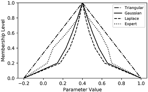
Figure 1. Examples of possible shapes of the membership function for a fuzzy number describing possible values of an arbitrary parameter. Functions for a triangular (dash-dotted), transformed Gaussian (solid), transformed Laplace (dashed), and expert knowledge-informed (dotted) fuzzy number are shown. The transformed membership functions are derived using a crisp value μ_K = 0.4, and standard deviation σ = 0.2. All functions have a support width of 3σ.

Fuzzy numbers can be used to propagate uncertainty through a mathematical model by applying well established rules for performing arithmetic operations on them. Traditionally this has been done by applying interval arithmetic to individual membership levels (Kaufman and Gupta, 1985). However, this method has the drawback that uncertainty is overestimated in systems where a fuzzy-valued term appears more than once in the system's equations. This is because all possible values of the fuzzy term are considered for each instance of the fuzzy term, which results in “double-counting” (Hanss, 2005).

For systems where a fuzzy-valued term appears multiple times, arithmetic should be performed using the transformation method described by Hanss (2002). This method is used here, since parameterizations for wave-induced circulation, near surface current shear, and wind shear all depend on the fuzzy-valued wind velocity. In the transformation method, the fuzzy-valued terms in the system of equations are discretized into arrays describing all possible combinations of all possible values of these terms. The system can then be solved using element-wise operations on these arrays. We give a brief description of the general transformation method here. Interested readers may refer to Hanss (2002) and Hanss (2005) for a thorough summary.

Consider a system of equations with n independent fuzzy variables P_i, i = 1, ..., n. Each P_i consists of m + 1 membership levels $X_i^{(j)}$. Each membership level $X_i^{(j)}$ is described by the interval $[a_i^{(j)},b_i^{(j)}]$, which is then discretized into an array ${\widehat{X}}_i^{(j)}$ according to the following equations.

$\begin{array}{ll}{P}_i=\left\{X_i^{(0)},X_i^{(1)},...,X_i^{(m)}\right\}& (\mathrm{14a})\end{array}$

$\begin{array}{ll}{X}_i^{(j)}=\left[a_i^{(j)},b_i^{(j)}\right],a_i^{(j)}\le b_i^{(j)}& (\mathrm{14b})\end{array}$

$\begin{array}{ll}{\widehat{X}}_i^{(j)}=\stackrel{{(m+1-j)}^{i-1}\text{ tuples of length }(m+1-j)}{\overbrace{({\gamma }_{1,i}^{(j)},{\gamma }_{2,i}^{(j)},...,{\gamma }_{(m+1-j),i}^{(j)},...,{\gamma }_{1,i}^{(j)},{\gamma }_{2,i}^{(j)},...,{\gamma }_{(m+1-j),i}^{(j)})}}& (\mathrm{14c})\end{array}$

$\begin{array}{ll}{\gamma }_{l,i}^{(j)}=\stackrel{{(m+1-j)}^{n-i}\text{ elements}}{\overbrace{(c_{l,i}^{(j)},...,c_{l,i}^{(j)})}}& (\mathrm{14d})\end{array}$

$\begin{array}{lll}{c}_{l,i}^{(j)}& =\{\begin{array}{ll}{a}_i^{(j)}& \text{for }l=1\text{ and }j=0,1,...,m\\ \frac{1}{2}\left(c_{l-1,i}^{(j+1)}+c_{l,i}^{(j+1)}\right)& \text{for }l=2,3,...,m-j\text{ and }\\ & j=0,1,...,m-2\\ b_i^{(j)}& \text{for }l=m-j+1\text{ and }j=0,1,...,m\\ \end{array}& (14e)\end{array}$

A graphical example of this discretization, adapted from Hanss (2005), is given in Figure 2 for a hypothetical fuzzy number described by four membership levels, i.e., m = 3. The final result of the transformation of all n fuzzy input variables P_i at one point in time is a set of m + 1 arrays ${\widehat{X}}_i^{(j)}$ for each P_i. To illustrate explicitly, consider a system of equations with two fuzzy input variables (i.e., n = 2), each similar to the example shown in Figure 2. The final arrays describing the membership level j = 1 are constructed as follows.

$\begin{array}{ll}{\widehat{X}}_1^{(1)}=\left[c_{0,1}^{(1)},c_{0,1}^{(1)},c_{0,1}^{(1)},c_{1,1}^{(1)},c_{1,1}^{(1)},c_{1,1}^{(1)},c_{2,1}^{(1)},c_{2,1}^{(1)},c_{2,1}^{(1)}\right]& (\mathrm{15a})\end{array}$

$\begin{array}{ll}{\widehat{X}}_2^{(1)}=\left[c_{0,2}^{(1)},c_{1,2}^{(1)},c_{2,2}^{(1)},c_{0,2}^{(1)},c_{1,2}^{(1)},c_{2,2}^{(1)},c_{0,2}^{(1)},c_{1,2}^{(1)},c_{2,2}^{(1)}\right]& (\mathrm{15b})\end{array}$

Using these arrays the system of equations for the membership level can be solved as it would be in a crisp manner, but using element-wise arithmetic on the arrays ${\widehat{X}}_1^{(1)}$ and ${\widehat{X}}_2^{(1)}$.

FIGURE 2

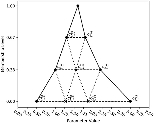
Figure 2. Illustration of the discretization of a fuzzy number into array form using the transformation method. Adapted from Hanss (2005).

The result of this element-wise arithmetic for each membership level (${\widehat{X}}_{result}^{(j)}$) can then be re-transformed into a fuzzy number by taking the minimum and maximum values of each ${\widehat{X}}_{result}^{(j)}$ to be the bounds of the membership level j of the fuzzy result, while ensuring that the fuzzy result remains convex.

$\begin{array}{ll}{P}_{result}=\left\{Z^{(0)},Z^{(1)},...,Z^{(m)}\right\}& (\mathrm{16a})\end{array}$

$\begin{array}{ll}{Z}^{(j)}=\left[a^{(j)},b^{(j)}\right]\text{,}j=0,1,...,m& (\mathrm{16b})\end{array}$

$\begin{array}{ll}{a}^{(j)}=min(a^{(j+1)},min({\widehat{X}}_{result}^{(j)}))& (\mathrm{16c})\end{array}$

$\begin{array}{ll}{b}^{(j)}=max(b^{(j+1)},max({\widehat{X}}_{result}^{(j)}))& (\mathrm{16d})\end{array}$

To apply this method to the prediction of drift trajectories, we begin by applying a probability-possibility transform to convert time series of measured ocean currents and winds at OSP into fuzzy numbers, using (Equation 13) as detailed in the following section. Each value in the resulting fuzzy time series is then transformed into arrays describing each membership level of the currents and winds, ${\widehat{X}}_{{\overrightarrow{u}}_c}^{(j)}(t)$ and ${\widehat{X}}_{{\overrightarrow{u}}_w}^{(j)}(t)$, according to Equation (14). The fuzzy-valued time series of drift speed, ${\widehat{X}}_{\frac{d\overrightarrow{x}}{dt}}^{(j)}(t)$ can then be derived by substituting ${\widehat{X}}_{{\overrightarrow{u}}_c}^{(j)}(t)$ and ${\widehat{X}}_{{\overrightarrow{u}}_w}^{(j)}(t)$ into (Equation 6) and re-transforming each value in ${\widehat{X}}_{\frac{d\overrightarrow{x}}{dt}}^{(j)}(t)$ into a fuzzy number according to Equation (16).

$\begin{array}{r}{\widehat{X}}_{\frac{d\overrightarrow{x}}{dt}}^{(j)}(t)={\widehat{X}}_{{\overrightarrow{u}}_c}^{(j)}(t)+\Delta {\overrightarrow{u}}_c{|}_{z=z_c}^{z=z_{drifter}}\left({\widehat{X}}_{{\overrightarrow{u}}_w}^{(j)}(t)\right)+{\overrightarrow{u}}_{stokes}\left({\widehat{X}}_{{\overrightarrow{u}}_w}^{(j)}(t)\right)\\ +\alpha \left({\widehat{X}}_{{\overrightarrow{u}}_w}^{(j)}(t)+\Delta {\overrightarrow{u}}_w{|}_{z=z_{drifter}}^{z=z_w}\left({\widehat{X}}_{{\overrightarrow{u}}_w}^{(j)}(t)\right)\right)& (17)\end{array}$

As described above, Equation (17) is solved using element-wise array arithmetic. The term $\Delta {\overrightarrow{u}}_c{|}_{z=z_c}^{z=z_{drifter}}\left({\widehat{X}}_{{\overrightarrow{u}}_w}^{(j)}(t)\right)$ is derived by applying the procedure described in section 2.2 to all elements of ${\widehat{X}}_{{\overrightarrow{u}}_w}^{(j)}(t)$. Similarly, ${\overrightarrow{u}}_{stokes}\left({\widehat{X}}_{{\overrightarrow{u}}_w}^{(j)}(t)\right)$ and $\Delta {\overrightarrow{u}}_w{|}_{z=z_{drifter}}^{z=z_w}\left({\widehat{X}}_{{\overrightarrow{u}}_w}^{(j)}(t)\right)$ are derived by element-wise solution of the procedures in sections 2.1 and 2.3, respectively. The procedure by which the resulting fuzzy-valued drift velocities are integrated to give the set of all possible displacements is described in section 3.3.

3.2. Fuzzification of Input Data

Fuzzy forms of observed currents and winds can be derived by considering the energy at scales unresolved by the observations, as well as the associated instrument uncertainties. To estimate the energy at time scales that are not resolved in the current and wind measurements, we fit a power law Af^−B to the high-frequency tail of the energy spectra of the currents and winds, defined as $P(f)=\frac{1}{2}(P_u(f)+P_v(f))$ where P_u/v(f) are the component spectra in the u/v directions. The unresolved energy between the Nyquist frequency, $f_N=\frac{1}{2d{t}_{obs}}$, and the frequency corresponding to the model timestep, $f_C=\frac{1}{2d{t}_{model}}$, can be estimated by log-linearly extrapolating the fitted power law to f_C, integrating from f_N to f_C, and finding the associated velocity scale by converting the resulting variance to amplitude, A_v.

$\begin{array}{ll}{A}_v=\sqrt{2{\sigma }^2}=\sqrt{2}{\left({\displaystyle {\int }_{f_N}^{f_C}}A{f}^{-B}df\right)}^{\frac{1}{2}}& (18)\end{array}$

In order to later derive the possible time series of drift velocity, the amplitude of the maximum unresolved accelerations, A_a, can be similarly derived by differentiating the extrapolated velocity energy spectrum. Here,

$\begin{array}{ll}{A}_a=\sqrt{2}{\left({\displaystyle {\int }_{f_N}^{f_C}}A{f}^{-(B-2)}df\right)}^{\frac{1}{2}}& (19)\end{array}$

Uncertainty due to spatial variability in the currents fields can only be estimated from numerical model results, or similar products, as observations of currents are only available in a single location. This uncertainty is denoted by σ_s, and the derivation is discussed in section 5.1 as it is case-specific.

To fuzzify the observed currents and winds we then assume that the uncertainty is isotropic, and that the uncertainties in the u and v directions are uncorrelated. The probability-possibility transform (Equation 13) can then be applied to each component separately, using the measured value as the crisp value. The standard deviation of the probability density function to be transformed is taken as the sum of A_v, σ_s, and the instrument uncertainty, σ_i. The approach taken here only requires the assumption of one distribution to describe the total uncertainty (discussed in section 5.1). A support width of $b^{(0)}-a^{(0)}=6(A_v+{\sigma }_s+{\sigma }_i)$, centered on the crisp value was selected, and the bounds of the intermediate membership levels were derived from Equation (13). Once the input variables have been expressed in fuzzy form they are used to solve for the fuzzy drift velocity by Equation (17), which is then integrated to derive the possible displacement of the drifting object.

3.3. Integration of Fuzzy Drift Velocities

The fuzzy set of all possible displacements can be derived by integrating all possible time series of drift velocity within a membership level that adhere to the maximum unresolved acceleration A_a. For each membership level below the crisp solution these time series can be found by first discretizing the membership level at the initial time into a number of starting points, n_S. From each starting point, n_p possible values at the next time step are determined based on the maximum unresolved acceleration and the bounds of the membership level. For each subsequent time step, n_p further possible values are determined from each possible value at the current time step, until the last time step is reached.

Letting the fuzzy drift velocity $P_{\frac{d\overrightarrow{x}}{dt}}=Z$ for notational simplicity, a possible value $Z_{k,t}^{(j)}$ (i.e., within membership level j, originating from starting point k, at time t) results in the following possible values at the next time step.

$\begin{array}{ll}{Z}_{k,t+1}^{(j)}(n)=Z_{k,t}^{(j)}+\Delta Z^{(m)}+\Delta Z^{(j)}(n),\text{ for }n=1,2,...,n_p& (\mathrm{20a})\end{array}$

$\begin{array}{ll}\Delta Z^{(m)}=Z_{t+1}^{(m)}-Z_{t+0}^{(m)}& (\mathrm{20b})\end{array}$

$\begin{array}{ll}\Delta Z^{(j)}(n)=6A_a{F}^{(j)}(n)\Delta t& (\mathrm{20c})\end{array}$

$\begin{array}{ll}{F}^{(j)}(n)=\frac{\frac{1}{2}(n_p+1)-n}{\frac{1}{2}(n_p-1)}\frac{b_{t+1}^{(j)}-a_{t+1}^{(j)}}{b_{t+1}^{(0)}-a_{t+1}^{(0)}}& (\mathrm{20d})\end{array}$

$\begin{array}{ll}{a}_{t+1}^{(j)}\le Z_{k,t+1}^{(j)}\le b_{t+1}^{(j)}& (20e)\end{array}$

Here Δt = dt_model is the model time step, $a_t^{(j)}$ and $b_t^{(j)}$ are the lower and upper bounds of membership level j at time t, and Z^(m) is the crisp time series of predicted drift velocities. All other symbols are as previously defined. A schematic of the process detailed in Equation (20) is shown in Supplementary Figure 2.

Integrating all unique crisp time series in the resulting set, using the forward Euler method, gives the set of all possible drifter displacements within this membership level $P_{\overrightarrow{x}}^{(j)}$ at time T = NΔt. This is written as follows

$\begin{array}{r}{P}_{\overrightarrow{x}}^{(j)}={\displaystyle \sum _{t=1}^{N-1}}\frac{1}{2}\left(Z_{m,t+1}^{(j)}(n)+Z_{m,t}^{(j)}\right),\text{ for }n=1,2,...,n_p\\ ,\text{ and }m=1,2,...n_S& (21)\end{array}$

In this case, use of the forward Euler method does not impact the results negatively, due to the assumption that the forcing fields are free of spatial variability. This will change when extending this analysis to include data from numerical ocean and atmospheric models and the associated spatial interpolation.

3.4. Model Evaluation

3.4.1. Skill Score

Drift trajectory models are generally evaluated for their ability to predict a drifting objects position at a snapshot in time (Molcard et al., 2009), as well as their ability to predict the complete path the object took to arrive at this position (Liu and Weisberg, 2011). The latter is a more difficult test, as it requires that the timing, magnitude, and direction of forcing events are captured correctly, whereas the former only requires that the cumulative effect of forcing events up to the time the snapshot is taken is correct. For the purposes of this paper we only evaluate the model performance at snapshots in time.

Our evaluation of model skill is based on the approach outlined in Molcard et al. (2009) and also used in Nudds et al. (2020). We adapt the approach for application to fuzzy results as follows. Model skill is calculated as a weighted sum across the membership levels, j = 0, 1, ..., m. Predictions with no skill receive a score of zero, while a perfect prediction receives a score of one.

$\begin{array}{ll}Skill=\frac{\left(1+\beta \right)\left(1-min\left(1,\frac{s}{d_{obs}}\right)\right)+{\displaystyle {\sum }_{j=0}^{m-1}}\left(f_j\frac{j}{m}+\beta \right)min\left(1,\frac{d_j}{X_{dj}}\right)}{{\displaystyle {\sum }_{j=0}^m}(\frac{j}{m}+\beta )}& (22)\end{array}$

The distances relevant to Equation (22) are illustrated in Figure 3. The first term in the numerator is the crisp instantaneous skill score, as in Nudds et al. (2020). The distance between the observed and modeled drifter positions, s, is normalized by the distance the observed drifter has traveled, d_obs, since a prediction within a fixed s should be considered more skillful as d_obs increases (Liu and Weisberg, 2011). This instantaneous skill score becomes zero if s > d_obs. β is a positive constant (arbitrarily set to 0.1 here) to ensure some skill is assigned to the predictions in the lowest membership level (j = 0). The exact value of β is unimportant.

FIGURE 3

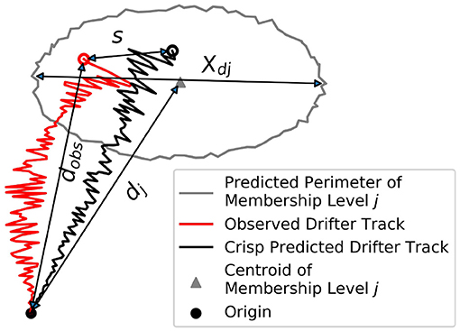
Figure 3. Illustration of instantaneous fuzzy skill score for trajectory evaluation. For clarity only a single membership level is shown.

The second term in the numerator is added to assign skill for each membership level $P_{\overrightarrow{x}}^{(j)}$ that contains the observed position. f_j is set equal to $-\beta \frac{m}{j}$ if the observed drifter is not within membership level j, and equal to 1 otherwise. To ensure that overestimation of uncertainty negatively impacts skill scores, scores are reduced proportionally to the ratio of the distance across the membership level, X_dj, and the mean displacement of the predicted drifter positions within the membership level d_j. A time series of skill can be derived by solving Equation (22) for each model time step.

3.4.2. Leeway Model Comparison

To contextualize the performance of the proposed drift prediction scheme we compare our results to analogous predictions made using the commonly used leeway method (Breivik and Allen, 2008; Breivik et al., 2011, 2013). In this method, the drift of an object is described as the sum of it's downwind, crosswind, and current-driven motion. The wind-driven component of the motion is object-specific and described using a set of nine coefficients, empirically determined for each object (Allen and Plourde, 1999; Breivik et al., 2011), which describe linear fits of the motion to the downwind, left-crosswind, and right-crosswind components of the motion along with error terms around these fitted values. Uncertainty is considered by perturbing the error terms using a Monte Carlo scheme (Breivik and Allen, 2008). For more details on the leeway method, interested readers are referred to Breivik and Allen (2008) and other works referenced herein.

The trajectories of each drifter type were simulated using the formulation of the leeway model in the OpenDrift trajectory modeling suite (Dagestad et al., 2018), by choosing the leeway object class which most closely corresponds to each drifter type (given in section 4). Simulations were performed using an ensemble of 5,000 particles released in a 100 m radius around the deployment site of the drifters.

For quantitative comparison of the proposed fuzzy number—based method with the leeway method, the results of the leeway method were described as a fuzzy number to enable scoring using the algorithm presented in the previous subsection. To convert the distributions of the 5,000 simulated particles into a fuzzy number, the relative particle density was calculated on a 1 km horizontal grid and this gridded density was then converted to a 2-dimensional fuzzy number by a slight modification of the algorithm presented by Khan and Valeo (2016), which enables the construction of fuzzy numbers from histograms of observed scalar data. Here the binned data comprising the histogram is sorted from largest to smallest bin count, and a membership of 1.0 is assigned to the coordinates of the bin with the largest count. The membership at coordinates corresponding to bins with lower counts is determined as the sum of the relative observation density in all bins lower than that under consideration to satisfy the consistency principle. For a detailed description of this method of constructing fuzzy numbers please refer to Khan and Valeo (2016). To adapt this method to two dimensional data, the coordinates of the bin centers were expressed as a complex number ${\overrightarrow{x}}_{bin}=x_{bin}+i{y}_{bin}$ and fixed membership levels were determined by delineating the area encompassing all bins with membership greater than or equal to the chosen level. Scoring of the leeway simulations was conducted according to section 3.4.1 once the simulated particle distribution was fuzzified in this manner.

4. Forcing and Verification Data

The observational data used to test the methods presented in sections 2 and 3 was collected near Ocean Station Papa (OSP) in the northeast Pacific during the period Feb 19–Mar 3, 2015. OSP (50.1°N, 144.9°W) has been the site of meteorological and oceanic observations since the early 1940's, and currently hosts a moored observation platform operated by the Ocean Climate Stations Office of NOAA/PMEL (Freeland, 2007). Detailed descriptions of the circulation and water properties at OSP are given in publications such as Pelland et al. (2016) and Cummins and Ross (2020). We make use of measurements of currents and winds recorded at the moored observation platform during a release of 44 ocean surface drifters nearby. The drifter tracks, as well as time series of the winds and currents measured at OSP, are shown in Figure 4.

FIGURE 4

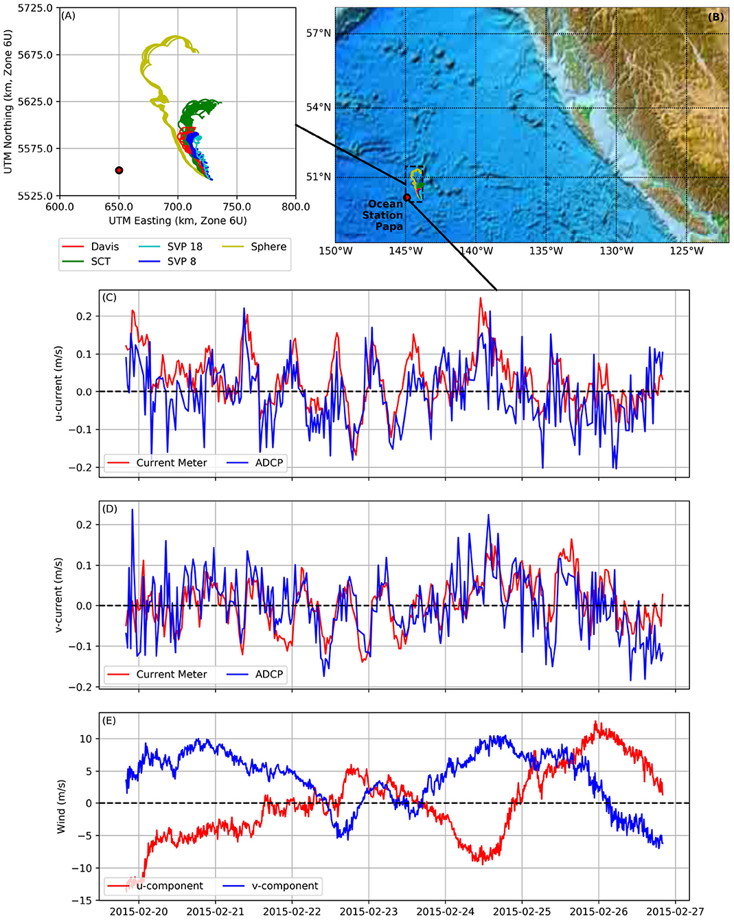
Figure 4. Tracks of drifters for 7 days after deployment near Ocean Station Papa (A,B), and time series of u,v components of currents (C,D) and wind (E) during the deployment.

Near-surface currents at OSP are recorded by a single-point 2 MHz Nortek Aquadopp current meter moored in a taut-line configuration at 15 m depth as well as a down-ward looking 300 kHz RDI Sentinel ADCP at 2 m below the water surface. Both instruments sample data over a period of 2 min. The current meter reports data at 10 min intervals, while ADCP profiles are reported at 30 min intervals (National Oceanic and Atmospheric Administration, Pacific Marine Environmental Laboratory, 2020a). The reported current meter accuracy is ±(1% of velocity + 0.5 cms⁻¹), while the accuracy of the ADCP is reported as ± 0.5 cms⁻¹. Both sensors have a resolution of 0.1 cms⁻¹. Winds are recorded 4 m above the water surface by a Gill Windsonic anemometer and averaged to 10 min intervals, with a reported accuracy of ± 2% (3%) of the speed (direction) reading, and a resolution of 0.01 ms⁻¹ (1°) (National Oceanic and Atmospheric Administration, Pacific Marine Environmental Laboratory, 2020b).

The current meter record at 15 m depth (Figures 4C,D) initially shows northeastward flow in response to northwesterly winds (Figure 4E), consistent with descriptions of wind-driven flow in the upper ocean dating back to Ekman (1905). As winds slacken between midday on Feb 21 and the evening of Feb 23, signals consistent with inertial oscillations appear in the current data.

Visual comparison of the current meter record with data from the closest ADCP measurement (centered at 16 m depth) during the first 7 days of the experiment (Figures 4C,D) reveals that the current meter indicates higher amplitude of low frequency fluctuations in the flow, and shows less spiking than the ADCP. A more detailed comparison (included in the section 1.2 of the Supplementary Material) reveals further differences between the two instruments. The current meter records a northeastward mean flow of ~ 3–4 cms⁻¹, while the mean flow recorded by the ADCP is much smaller and in the opposite direction. This appears to be a systematic discrepancy between the two instruments. Differences between the two instruments could be due to interference from the point current meter on the beams of the ADCP (Nathan Anderson, PMEL, personal communication, September 2021) or due to the differences in operating frequency and sampled volume of water (Richard Thomson, DFO, personal communication, September 2021). Drifter trajectories are computed and assessed using the data from both instruments, in order to test which instrument provides more relevant information.

On February 19, 2015 at approximately 20:30H UTC, 44 ocean surface drifters of five different geometries were deployed approximately 75 km east of OSP. These included the following: 8 Sphere drifters which float mostly above the water surface; 28 Surface Circulation Tracker (SCT) (Oceanetic Measurement Ltd., 2016) drifters which float in the upper 37.5 cm of the water column and have been shown to reasonably reproduce oil sheening (Blanken et al., 2020); 3 Davis drifters (Davis, 1985) which float in the upper 1.5 m of the water column and are similar to the SLDMB drifters commonly used for search and rescue applications; and 5 drifters based on the Surface Velocity Program (SVP) design (Poulain and Niiler, 1989; Niiler et al., 1995), 4 with the 4.6 m holey-sock drogue starting at ~8 m depth (hereafter SVP 8) and one starting at ~18 m (hereafter SVP 18). SVP drifters are generally used to map near-surface ocean circulation. One of the SCT drifters failed shortly after deployment. Pictures of the drifters and their idealized geometry and drag coefficients are shown in Figure 5. Most drifters transmitted data until Mar 3, 2015, however we only consider the first 7 days of the deployment in this study. During this time drifters were within 55–150 km of OSP (Supplementary Figure 3). To simulate the trajectories of these drifter types using the leeway method, the following object types were chosen as proxies: Sphere − > bait box (lightly loaded); SCT − > WW2 mine; Davis − > oil drum; SVP (8 and 18 m) − > person-in-water floating vertically. The corresponding leeway coefficients are reproduced in Supplementary Table 1.

FIGURE 5

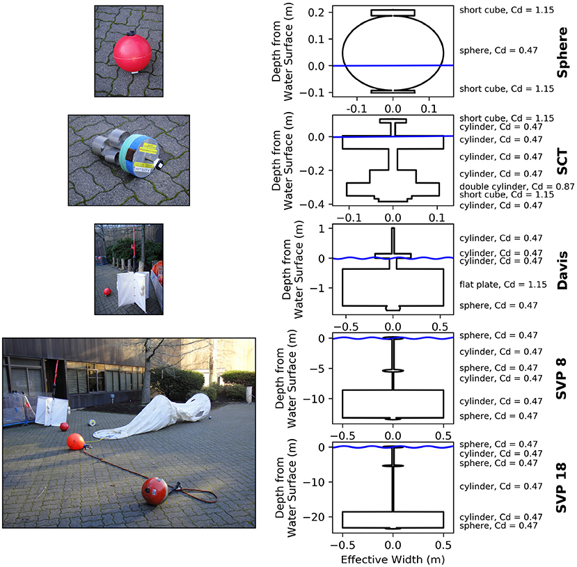
Figure 5. The drifters deployed for this study (left), and their idealized geometry, including approximate drag coefficients (right). The SVP 8 (bottom-left photograph) and SVP 18 drifters (no photograph shown) are identical except for the length of the tether.

All drifters followed a mean northeastward trajectory during the first 5 days of their deployment (Figure 4A), consistent with the mean wind direction during this time, with a change to westward drift coincident with a change in the wind direction. The lengths of the trajectories are inversely related to drogue depth of the drifter. The Sphere drifter trajectories are approximately twice as long as those of the SCT drifters, which are in turn longer than the Davis, SVP 8, and SVP 18 drifters. The latter three drifter types, which are drogued deeper in the water column, exhibit clockwise looping which is likely due to inertial oscillations like those noted in the current meter record.

5. Results

5.1. Fuzzy Forcing

Converting the current and wind record into fuzzy number equivalents using the procedures described in section 3.2 shows that the uncertainty in these measurements is appreciable once aggregated. To begin, we fit power laws to the tail of the wind and current meter spectra using log-transformed linear regression between frequencies $\frac{1}{2x7200sec}$ and the Nyquist frequency, f_N. The low-frequency threshold is chosen by visual inspection of the energy spectra (Supplementary Figure 4). The parameters to the regression Af^B as well as the amplitude of the unresolved velocities and accelerations according to Equations (18) and (19) are given in Table 1 for a model timestep dt_model = 300 s. The amplitude of the unresolved energy A_v is approximately three to five times the instrument uncertainty for the anemometer and the current meter but approximately 17 times larger for the ADCP. This is at least in part due to the longer output interval of the ADCP but also due to the shallower spectral slope that suggests additional noise at high frequencies, as was noted from visual inspection of the time series in section 4.

TABLE 1

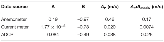
Table 1. Amplitude of energy in unresolved timescales and associated power law coefficients.

Uncertainty due to spatial variability is estimated by examining the current fields from the GLORYS12 ocean re-analysis. GLORYS12 is a state-of-the art hindcast numerical simulation of ocean conditions from 1993-present, with data assimilation of satellite altimetry and temperature measurements as well as in situ profiles of temperature and salinity (Lellouche et al., 2021). The modeled daily-mean currents at 15 m depth suggest significant spatial structure with maximum fluctuations in current amplitude of ~0.2 m/s over the duration of the experiment (see Supplementary Figure 5). Comparing the modeled currents at OSP to daily averages of the measurements from the current meter and ADCP suggests that at OSP the modeled currents are biased southeasterly by ~0.045 m/s with respect to the current meter, and easterly by ~0.05 m/s with respect to the ADCP. RMS errors of the modeled velocity components are ~0.04–0.06 m/s. A comparison of the modeled currents at the drifter locations with the modeled current at OSP also suggests that currents at OSP are directed more southeasterly than at the drifter locations, with a bias of ~0.075 m/s and RMS errors of 0.01–0.02 m/s for all drifters except the Sphere drifters which travel further and therefore sample more variability (see Supplementary Figures 3, 6). However, there is considerable uncertainty about the accuracy of the mean difference in the modeled currents between the drifter location and OSP given that this difference corresponds well with the identified bias in the currents at OSP. A plausible explanation is that the features shown in Supplementary Figure 5 may be slightly misaligned in the model. For the purpose of this paper, we approximate uncertainty due to spatial variability by taking σ_s = 0.015 m/s as the standard deviation of the differences between the modeled currents at OSP and the drifter locations. As the modeled currents leave some doubt about the relevance of the currents at OSP to the drifter locations, trajectories are computed with and without forcing from the measured currents as is later discussed in section 5.2. Further assessment of the modeled surface dynamics in GLORYS12 can be found in Lellouche et al. (2021). As noted previously, the effect of uncertainty in modeled ocean currents on trajectory prediction will be further investigated in future work.

Once uncertainties have been quantified, the current and wind data are converted to a fuzzy number using the probability-possibility conversion in Equation (13). We expect that the uncertainty due to unresolved time scales will follow a distribution that is similar to that obtained by simulating a red noise process with an f^B spectral slope and variance corresponding to the sum of A_v, σ_s, and σ_i (shown for the current meter record in Supplementary Figure 7). This distribution is better represented by a Laplace distribution than by a Gaussian distribution, though both overestimate the tails. The random instrument uncertainty is more likely to follow a Gaussian distribution. Since the unresolved energy in the current data, especially for the ADCP, is significantly larger than the instrument uncertainty we convert it to fuzzy numbers using a Laplace distribution, while a Gaussian distribution is chosen for the wind record. The effect of the choice of distribution should be further investigated, however this is beyond the scope of the current study. Applying Equation (13) with the above distributions, A_v from Table 1, σ_s from above, σ_i from section 4, and four equally spaced membership levels on the interval [0, 1], i.e. m = 3, yields the fuzzy time series shown in Figures 6A–D. The number of membership levels is limited by the computational expense of the current shear calculation. This may be mitigated by employing alternative parameterizations for current shear, however a detailed comparison of possible parameterizations is beyond the scope of the current work.

FIGURE 6

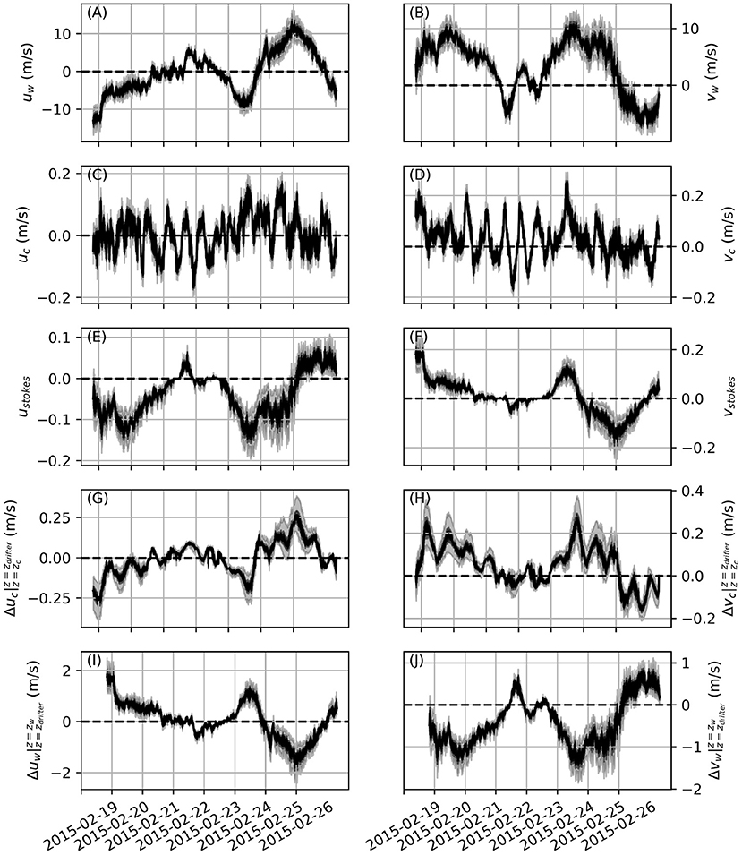
Figure 6. Components of fuzzy wind (A,B), current (C,D), Stokes drift (E,F), current shear (G,H), and wind shear (I,J) for the first 7 days of the drifter deployment. The crisp value (measurement) is shown in black and the three fuzzy membership levels are indicated in grayscale. For clarity in (E–J) only values for SCT drifters with the velocity profile applied by the “centroid” scheme are shown.

The fuzzified winds and currents exhibit uncertainties that at times exceed 5 m/s for winds and 0.2 m/s for currents at the lowest membership level, during times when winds and currents are strong. The influence of the relative instrument uncertainty on overall uncertainty is clearly seen in the reduced width of the fuzzy numbers when wind speeds are low, between midday on Feb 22 and midday on Feb 23 (Figure 6).

Transforming the fuzzy winds according to Equation (14) allows us to calculate fuzzy values of Stokes drift, current shear, and wind shear according to the procedures outlined in sections 2.1 and 2.2. The time series of these fuzzy vectors are shown in Figures 6E–J. Here only values for SCT drifters derived using the centroid method (Equation 7a) are shown for clarity. These variables were calculated for each drifter separately by each of the three methods of applying the shear profile given in Equation (7). Stokes drift and current shear on the near-surface SCT drifters are strongly positively correlated with the wind velocity, though both diminish significantly when wind speeds are below ~5 m/s. During times of strong winds both Stokes drift and current shear are comparable to, or larger than, the measured currents. These terms are therefore expected to have first order impacts on the drift trajectory prediction, consistent with the findings of Röhrs et al. (2012). During strong winds the magnitude of the uncertainty (i.e., the width of the lowest membership level) in the estimated Stokes drift and current shear is comparable to the magnitude of the estimate itself.

Wind shear appears to be a minor factor compared to Stokes drift and current shear. As expected, $\Delta {\overrightarrow{u}}_w{|}_{z=z_{drifter}}^{z=z_w}$ is inversely correlated with wind velocity, i.e., it reduces the effective wind velocity in Equation (17). The magnitude of wind shear is at most ~20% of the wind speed, and subject to similar relative uncertainties as Stokes drift and current shear.

5.2. Optimal Forcing Combinations

Drift trajectories were computed for all combinations of forcing terms on the right-hand side of Equation (17), methods of applying sheared forcing as per Equation (7), and sources of current data (current meter or ADCP). Trajectories were then scored at each time step using Equation (22) to determine the optimal combination of parameters by identifying the combination giving the highest skill score at each time step. We consider a forcing term to be part of the optimal solution if it is present in the solution with the highest skill score, for at least 50% of time steps. Wind shear is only considered during times when wind drag is an important forcing term, however current shear may be considered independently of measured currents. The optimal combination of forcing terms as a function of time is summarized for each drifter in Figure 7. The percentage of time each of the three methods of applying profile shear (Equations 7a–c) was most suitable is summarized in Figure 8. The optimal parameters for each drifter, and the trajectories predicted using these parameters, are shown in Figures 9–13.

FIGURE 7

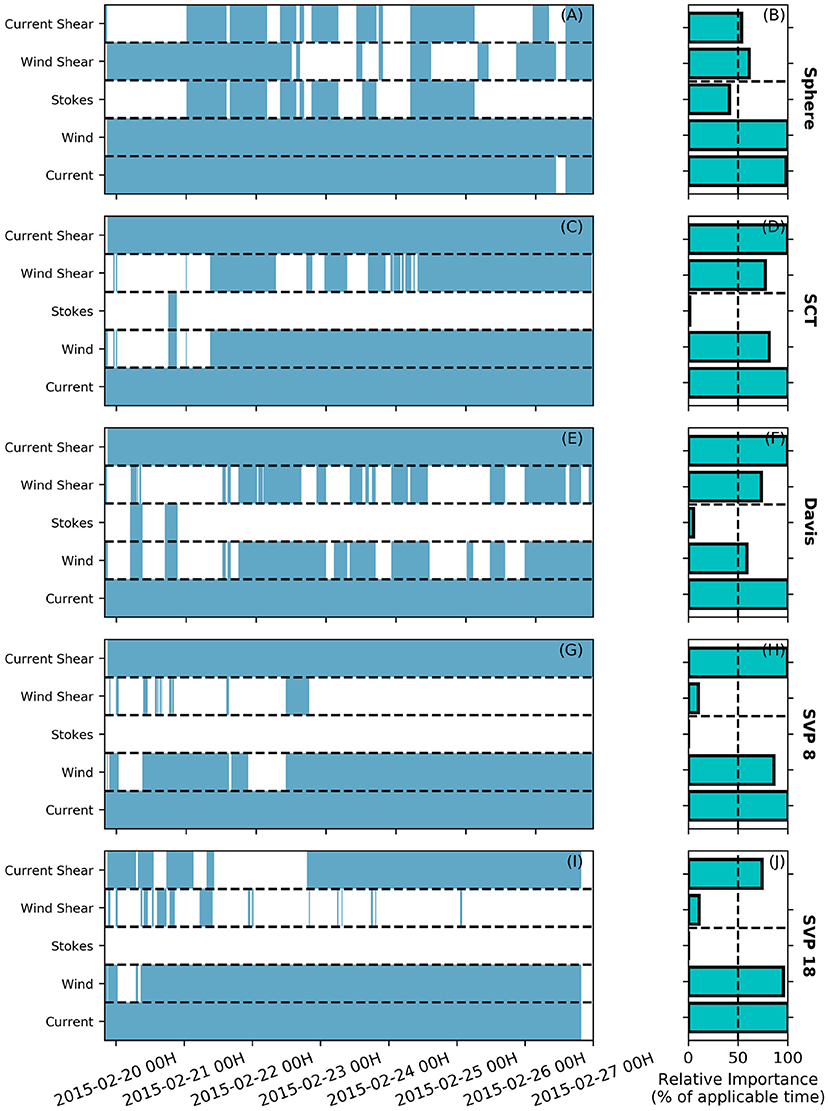
Figure 7. Summary of optimal forcing terms for each drifter as a function of time. In the left-hand (A,C,E,G,I), timesteps where a forcing term contributed to the solution achieving the highest skill score are shaded in blue for each drifter type. In the right hand (B,D,F,H,J) the percentage of applicable time each forcing term contributed to the optimal solution is summarized.

FIGURE 8

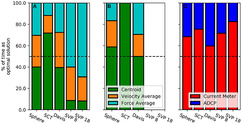
Figure 8. Percentage of time current shear (A) and Stokes drift (B) profiles applied via the centroid and area-weighted average of velocity or force produce the optimal solution for a the trajectories of each of the five drifters. No results are shown for Stokes drift on the SVP drifters, as the analysis indicates that Stokes drift does not contribute to the optimal trajectory prediction at any time. (C) Shows the percentage of time the currents measured by the current meter (red) and the ADCP (blue) contribute to the optimal solution.

FIGURE 9

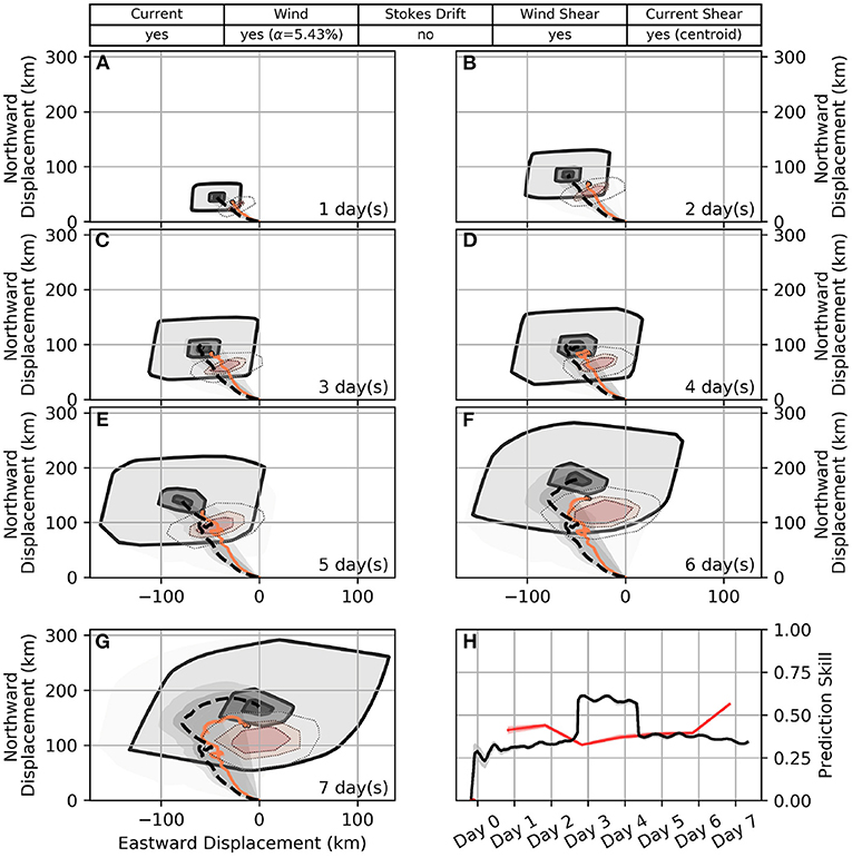
Figure 9. Daily predicted tracks of the sphere drifters for 7 days after deployment using the indicated optimal forcing combination (A–G), and a time series of model skill during this period (H). Membership levels of the possible displacement, $P_{\overrightarrow{x}}^{(j)}$ for j = 0, 1, 2, are indicated in grayscale shading, increasing in intensity toward the crisp solution (j = 3) which is indicated by the dashed black line. Equivalent results obtained using the leeway method are shown in red shading. Observed drifter tracks are superimposed in orange. Model skill is also shown in grayscale for the optimal forcing combination and in red for the leeway method. Shading indicates the maximum and minimum skill for the ensemble of drifters, while the solid line indicates the mean. Red markers on the x-axis of the skill plot indicate times when at least one observed drifter fell outside of the lowest membership level.

FIGURE 10

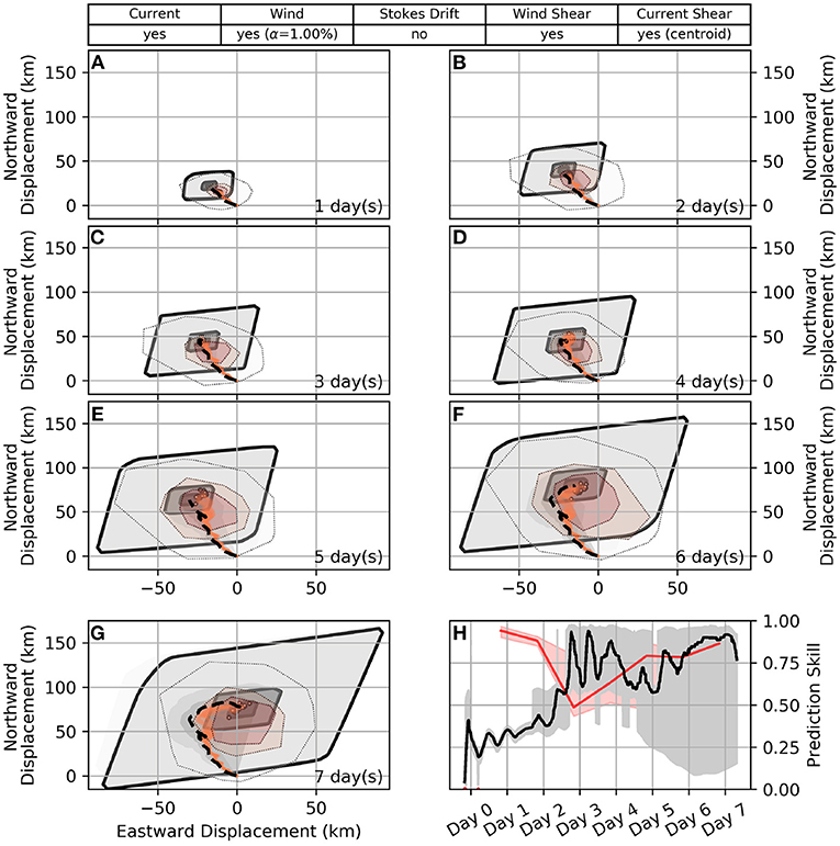
Figure 10. Daily predicted tracks of the SCT drifters for 7 days after deployment using the indicated optimal forcing combination (A–G), and a time series of model skill during this period (H). Same layout as Figure 9.

FIGURE 11

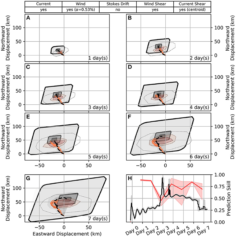
Figure 11. Daily predicted tracks of the Davis drifters for 7 days after deployment using the indicated optimal forcing combination (A–G), and a time series of model skill during this period (H). Same layout as Figure 9.

FIGURE 12

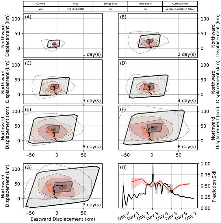
Figure 12. Daily predicted tracks of the SVP 8 drifters for 7 days after deployment using the indicated optimal forcing combination (A–G), and a time series of model skill during this period (H). Same layout as Figure 9.

FIGURE 13

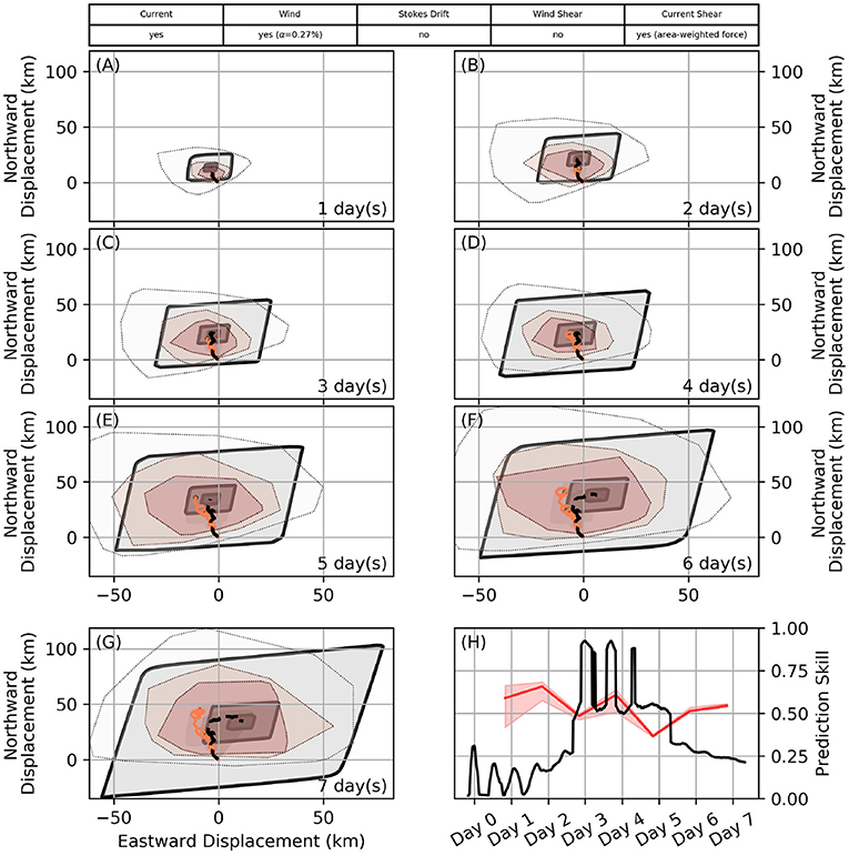
Figure 13. Daily predicted tracks of the SVP 18 drifters for 7 days after deployment using the indicated optimal forcing combination (A–G), and a time series of model skill during this period (H). Same layout as Figure 9.

Current, wind, and current shear all play an important role in predicting the trajectories of the drifters, and wind shear is an important term for the near-surface drifters (Sphere, SCT, and Davis) (Figure 7). This suggests that the importance of wind shear increases with the magnitude of the wind drag term. Since forcing from measured currents is consistently part of the optimal solution, we conclude that currents measured at OSP are relevant to the drifter location, despite the separation between these locations. In 60–80% of instances, forcing with the currents measured by the current meter produced a better solution than forcing with currents measured by the ADCP (Figure 8C). This is likely due to the higher reporting frequency (every 10 min for current meter compared to every 30 min for ADCP), as well as the possible high frequency noise in the ADCP record discussed earlier. Stokes drift is not part of the optimal solution for any drifter type. It is more frequently of importance for the near-surface drifters however, and not important at any time for the SVP drifters. A possible explanation is that Stokes drift may lag behind wind forcing as the wave field responds to changes in the wind. In general, the potential effects of Stokes drift should be further investigated by a sensitivity analysis to both different methods of calculating Stokes drift as well as time-lagged methods of applying this forcing. The optimal forcing terms are often simultaneously applicable in the latter half of the simulation period, however this is less likely to be the case during the first half of the simulation period. A possible explanation for this is that the lower winds during the first half of the simulation period result in more small scale current variability, such as inertial oscillations, which are not captured in the measurements at OSP.

The deterministically derived wind drag factor, α, from Equation (5) produces appropriate results. Values of α are 5.43, 1.00, 0.53, 0.28, and 0.27% for the Sphere, SCT, Davis, and SVP 8 and 18 drifters, respectively. The values calculated for the SVP drifters agree well with the slippage estimate of 0.2% of the wind speed given by Poulain and Niiler (1989). To assess the sensitivity of the results to the wind drag factor, the changes in mean skill score for trajectory predictions made using values ranging from 0.5α to 1.5α are given in Table 2. For the near-surface drifters any increase in the wind drag factor degrades the predictions, while decreases in the wind drag factor can improve the prediction. This improvement is minor (maximum 5.5%) for the SCT and Davis drifters, but can be significant (up to 78% for a 25% reduction of α) for the Sphere drifters. This suggests that perhaps wind shear is underestimated here, which may be expected as winds are calculated at a 1 m reference height while the bulk of the exposed drifter parts are within 0.2 m of the water surface. It is also possible that some dynamics associated with objects that are primarily above the water surface are not captured here, as suggested by the significant differences in the Sphere drifter results. Altering the wind drag factor for the SVP drifter generally resulted in a negligible change to the results. Decreasing α generally resulted in a small (maximum 3.1%) decrease in skill while increasing α resulted in a similarly small (maximum 3.4%) increase in skill.

TABLE 2

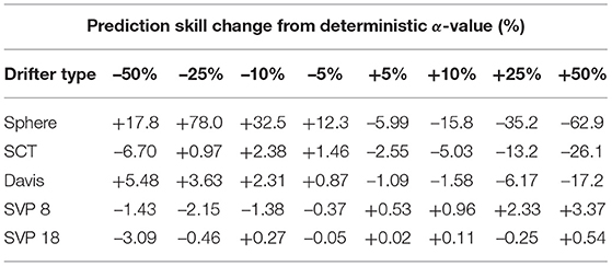
Table 2. Percent change in mean trajectory prediction skill for given adjustments to deterministic wind drag factor, α.

Optimal methods of applying sheared forcing vary by drifter type. For applying current shear, the centroid method produces the best results for near-surface drifters, while the area-weighted force method produces the best results for the SVP drifters (Figure 8A). The grouping of these results is likely in part due to the 1 m vertical discretization used in solving for the current shear, which results in approximately linear velocity profiles over the draft of the near-surface drifters as these are almost entirely in the uppermost vertical level. For the longer SVP drifters, the effect of nonlinearities in the vertical velocity profile becomes both more relevant and better resolved. The centroid method provides the best results for applying Stokes drift for all applicable drifter types (Figure 8B).

5.3. Trajectory Results

The optimal forcing combinations for each drifter lead to predictions that are skillful (i.e., the observed positions remain within the lowest membership level) for at least 7 days. The observed and predicted trajectories of the Sphere, SCT, Davis, SVP 8, and SVP 18 drifters as well as the time series of model skill associated with the prediction are shown in Figures 9–13. The analogous results from the leeway method and associated skill scores are also shown.

The trajectories of the near-surface drifters (Sphere, SCT, and Davis) are generally well predicted, especially for the SCT drifters (Figures 9–11). In the first 2 days of the simulation, the length of all three trajectories is slightly under-predicted, however the model results converge with observations by the third day. This convergence coincides with a shift in the winds from consistent winds toward the northwest to weaker and more variable winds. The predicted trajectories of the Sphere drifters consistently veer slightly to the west of the observations. On the fifth day of the simulations, the behavior of the three near-surface drifter types diverges. From here, the northward extent of the Sphere drifter trajectories is over-predicted and the predicted trajectories of the Davis drifters begin to shift eastward of the observations, while the predicted tracks of the SCT drifters remain close to the observations. Modeled tracks of both the Sphere and Davis drifters continue to propagate eastward at a higher rate than is observed on days 6–7, while the trajectories of the SCT drifters remain close to the observations. During this time the dispersion of the cluster of SCT drifters becomes comparable to the scale of the 0.67 membership level, which suggests that the size of these membership levels corresponds well with natural dispersion processes associated with unresolved high-frequency fluctuations in the forcing data.

The near-surface drifter locations predicted by the leeway method tend to be slightly to the southeast of the locations predicted by the proposed fuzzy method, with the observed positions in between the two sets of model results. The lowest membership level of the predicted positions is larger for the proposed fuzzy method than for the leeway method, while the intermediate membership levels are larger for the leeway method. Skill scores for the two models are quite similar. Whenever a particular model captures one or more of the observed positions in an intermediate membership level (0.33 or 0.67), its skill will rise above the other model temporarily. The skill of the leeway method is higher near the beginning and end of the simulation, however the proposed fuzzy method often has higher skill overall during the intermediate period due to the smaller intermediate membership levels.

For the more deeply drogued SVP drifters, the trajectory length is generally slightly under-predicted and the modeled trajectories also begin to veer eastward of the observations around the fourth day of the simulation. After this point, the modeled trajectories strongly diverge eastward of the observations. The center of the predicted positions is similar between the proposed fuzzy method and the leeway method however, contrary to the near-surface drifters, the membership levels of positions predicted by the leeway method are generally larger than those from the fuzzy method here. Again the skill score of the two methods is similar, with the leeway method scoring higher near the beginning and end of the simulation while the fuzzy method scores higher in the intermediate period.

6. Discussion

The fuzzy number based scheme for describing and propagating uncertainty in trajectory predictions proposed in this paper appears to work well, given that the predicted sets of possible displacements covered the observed position of the drifters. The scheme is advantageous in that it does not require specification of empirical coefficients, and can be applied anywhere concurrent measurements of wind and currents are available. Future work to extend the scheme to include forcing data from numerical models will further expand its utility. The work presented here can also be readily extended to arbitrary or unknown object geometries by describing the direct wind drag coefficient, α, as a fuzzy number.

Regarding the representation of uncertainty, it is worthwhile to consider whether displacements in the lowest membership level should be reported, given that they are representative of the largest displacements thought to be possible, without making claims about the probability of such displacements (by definition of a possibility distribution). It is noted that the lowest membership level at times overestimated the uncertainty of predicted positions, which is to be expected as the probability density functions transformed to derive the fuzzy currents and winds were noted to overestimate the extreme values (i.e., the tails) of the represented uncertainty. The form of the input fuzzy numbers clearly affects the results of the trajectory model, similar to previous results from Khan et al. (2013). Increasing the number of membership levels in future work may help resolve this question by better resolving the skill score and the lowest membership level containing observed drifters. However, increasing the number of membership levels comes with significant increases in computational demands, and the 'lowest useful' membership level will always vary as a function of the forcing data quality.

Direct wind drag is a dominant forcing factor on all considered drifter types, and it is shown that a deterministic, geometry-based wind drag coefficient leads to skillful predictions for at least 7 days when the uncertainty in the forcing data is propagated through the prediction (Figures 9–13). However, the determined wind drag coefficients at times over-predicted the trajectory length for near-surface drifters and lower values of α would have resulted in higher model skill. Conversely, for the SVP drifters trajectory lengths were slightly under-predicted even without the addition of Stokes drift and wind shear terms, and higher values of α would have resulted in slightly increased model skill (see Table 2). Therefore, some uncertainty remains around the processes relevant to the down-wind components of the motion, as direct wind drag, part of the current shear, and Stokes drift act co-linearly and their relative importance is less clear when the uncertainty in the wind forcing is accounted for. Due to this ambiguity in the co-linear forcing terms, a single set of leeway coefficients describing the down-wind motion was noted as beneficial in Breivik et al. (2011). However, within the framework proposed here, further sensitivity analysis of the parameters of the Stokes drift and current shear parameterizations in the proposed method may provide clarification of this ambiguity, though this is beyond the scope of the current paper.

The model proposed here avoids the need to specify empirically determined leeway coefficients while retaining results of a similar quality to the commonly used leeway method. This is a clear benefit, as leeway coefficients are not available for every object type and may not be representative of an object for which no coefficients have been determined. This is evident when comparing the correspondence of the leeway and fuzzy results for near-surface and SVP drifters. For near-surface drifters the leeway method results in a smaller range of predicted possible positions at the lowest membership level, though the range of intermediate membership levels is larger. This is to be expected as the lowest membership level represents all possible solutions, which may not be realized during a simulation with 5,000 particles. For the SVP drifters however, the leeway method results in a larger area of possible displacements at all membership levels. For near-surface drifters closely aligned proxy objects are available, with leeway coefficients determined by the direct method (current measured during determination) (Breivik et al., 2011). For the SVP drifters, the closest available proxy object is a vertically oriented person in the water which in reality has a much shallower draft than the SVP drifters. The geometry of a vertical PIW is also quite variable, which is represented in the coefficients and results in a larger uncertainty than is predicted by the fuzzy method.

Closer comparison of the modeled and observed trajectories also suggests that not all physics governing the evolution of a drift trajectory are captured by the trajectory model proposed here. The inclusion of uncertainty compensates for this by capturing the resulting discrepancies in lower membership levels, but the effect of the missing physics remains evident. For four of the five drifter types, a significant eastward displacement is predicted during the last 2 days of the simulation, in response to a change in the winds. This displacement is not seen to the same extent in the observations, which may point to a lagged response to wind forcing or spatial variability in the winds between OSP and the drifter locations. The modeled trajectories also more generally tend slightly to the east (left) of the observed trajectories, which may be due to absence of Stokes drift forcing or due to the chosen values of the constants in the current shear parameterization. A sensitivity analysis of these parameters may yield further insight here, but is beyond the scope of the current study. Alternatively, this eastward tendency may suggest that Coriolis-Stokes forcing plays a role, as its inclusion is expected to deflect the surface current further to the right of the wind (Polton et al., 2005; Weber et al., 2015). This may be expected as our estimates of Stokes drift have a similar magnitude to the measured currents, consistent with the results reported by Röhrs et al. (2012). Most common ocean models include parameterizations of Coriolis-Stokes forcing (Röhrs et al., 2012), and therefore extending the method proposed here to numerical modeling results may achieve these improvements and also meet the obvious need for representation of spatial variability in the forcing fields.

7. Conclusions

Uncertainty in surface drift trajectory predictions is of significant importance when responding to marine contaminant spills and performing search and rescue operations, along with a plethora of other applications. We have presented a method for modeling the trajectories of drifting objects that makes use of fuzzy numbers to characterize the uncertainty inherent in these predictions without relying on specification of empirical dispersion coefficients or random kicks. A comparison of results from this method to observations from five different types of surface drifters suggests that the method works well, and offers similar performance as the frequently used, empirical leeway method. Following a deployment near Ocean Station Papa in the northeast Pacific, 44 observed drifters of five different types remain within the range of modeled possible displacements during the 7 days following their deployment.

Moreover, our results show that the response of drifting objects to direct wind forcing can be reasonably well predicted based on the objects geometry provided that wind-induced Stokes drift and current shear are appropriately parameterized. Even with these parameterizations, we find direct wind drag to be a forcing term of first order importance for all drifters considered here. A novel skill metric for assessing model performance proved to be a useful tool for identifying the optimal combinations of parameterizations. The analysis presented here can be extended to objects of arbitrary geometry, and also unknown or uncertainty geometry when α is expressed as a fuzzy number. Further development and evaluation will expand its utility by incorporating forcing data from numerical models.

Data Availability Statement

Publicly available datasets were analyzed in this study. This data can be found here: www.waterproperties.ca; www.pmel.noaa.gov/ocs/data/disdel/; https://resources.marine.copernicus.eu/?option=com_csw&view=details&product_id=MULTIOBS_GLO_PHY_REP_015_004.

Author Contributions

TJ: observation campaign. HB, CH, CV, and UK: conceptual design. HB, CV, and UK: method development. HB and CH: data analysis. HB and TJ: figures and tables. HB: writing. CV, CH, UK, and TJ: editing. All authors contributed to the article and approved the submitted version.

Funding

This work was supported through the Oceanography sub-initiative of the Government of Canada's Oceans Protection Plan. Collection of the drifter data was financially supported through the World Class Prevention, Preparedness and Response to Oil Spills from Ships Initiative of the Department of Fisheries and Oceans Canada. Environmental data collected at the Ocean Station Papa mooring was made available through the Ocean Climate Stations (OCS) Office of NOAA/PMEL.

Conflict of Interest

The authors declare that the research was conducted in the absence of any commercial or financial relationships that could be construed as a potential conflict of interest.

Publisher's Note

All claims expressed in this article are solely those of the authors and do not necessarily represent those of their affiliated organizations, or those of the publisher, the editors and the reviewers. Any product that may be evaluated in this article, or claim that may be made by its manufacturer, is not guaranteed or endorsed by the publisher.

Acknowledgments

We would like to thank the captain and crew of the CCGS John P. Tully, as well as the scientists aboard, for their hard work on the Line P program that made this study possible. We also thank the staff at the Ocean Climate Stations Office of NOAA/PMEL for their work in collecting observations at Ocean Station Papa, and the staff at E.U. Copernicus Marine Service Information for their work in compiling the GLORYS12 numerical model results. We thank both organizations for making these data publicly available. Finally, we would like to thank two reviewers, whose helpful comments and insight improved the quality of this manuscript.

Supplementary Material

The Supplementary Material for this article can be found online at: https://www.frontiersin.org/articles/10.3389/fmars.2021.618094/full#supplementary-material

References

National Oceanic and Atmospheric Administration, Pacific Marine National Oceanic and Atmospheric Administration Pacific Marine Environmental Laboratory (2020b). Seattle, WA: Ocean Station Papa: Sensor Specifications.

Allen, A. A., and Plourde, J. V. (1999). Review of leeway: Field experiments and implementation. Final Report CG-D-08-99, United States Department of Transportation and United States Coast Guard, Washington, DC.

Google Scholar

Blanken, H., Hannah, C., Klymak Jody, M., and Juhász, T. (2020). Surface drift and dispersion in a multiply connected fjord system. J. Geophys. Res. Oceans 125, e2019JC015425. doi: 10.1029/2019JC015425

CrossRef Full Text | Google Scholar

Breivik, Ø., and Allen, A. A. (2008). An operational search and rescue model for the Norwegian Sea and the North Sea. J. Mar. Syst. 69, 99–113. doi: 10.1016/j.jmarsys.2007.02.010

CrossRef Full Text | Google Scholar

Breivik, O., Allen, A. A., Maisondieu, C., and Olagnon, M. (2013). Advances in search and rescue at sea. Ocean Dyn. 63, 83–88. doi: 10.1007/s10236-012-0581-1

CrossRef Full Text | Google Scholar

Breivik, Ø., Allen, A. A., Maisondieu, C., and Roth, J. C. (2011). Wind-induced drift of objects at sea: the leeway field method. Appl. Ocean Res. 33, 100–109. doi: 10.1016/j.apor.2011.01.005

CrossRef Full Text | Google Scholar

Butler, J. (2015). Independent review of the M/V Marathassa fuel oil spill environmental response operation. Technical report, Canadian Coast Guard.

Google Scholar

Checkley, D. M., Raman, S., Maillet, G. L., and Mason, K. M. (1988). Winter storm effects on the spawning and larval drift of a pelagic fish. Nature 335, 346–348. doi: 10.1038/335346a0

CrossRef Full Text | Google Scholar

Cho, K.-H., Li, Y., Wang, H., Park, K.-S., Choi, J.-Y., Shin, K.-I., et al. (2014). Development and validation of an operational search and rescue modeling system for the Yellow Sea and the East and South China Seas. J. Atmos. Oceanic Technol. 31, 197–215. doi: 10.1175/JTECH-D-13-00097.1

CrossRef Full Text | Google Scholar

Clarke, A. J., and Van Gorder, S. (2018). The relationship of near-surface flow, Stokes drift and the wind stress. J. Geophys. Res. Oceans 123, 4680–4692. doi: 10.1029/2018JC014102

CrossRef Full Text | Google Scholar

Craig, P. D., and Banner, M. L. (1994). Modeling wave-enhanced turbulence in the ocean surface layer. J. Phys. Oceanogr. 24, 2546–2559. doi: 10.1175/1520-0485(1994)024andlt;2546:MWETITandgt;2.0.CO;2

CrossRef Full Text | Google Scholar

Cummins, P. F., and Ross, T. (2020). Secular trends in water properties at Station P in the northeast Pacific: an updated analysis. Progr. Oceanogr. 186:102329. doi: 10.1016/j.pocean.2020.102329

CrossRef Full Text | Google Scholar

Dagestad, K.-F., Röhrs, J., Breivik, Ø., and Ådlandsvik, B. (2018). Opendrift v1.0: a generic framework for trajectory modelling. Geosci. Model Dev. 11, 1405–1420. doi: 10.5194/gmd-11-1405-2018

CrossRef Full Text | Google Scholar

Daniel, P., Jan, G., Cabioc'h, F., Landau, Y., and Loiseau, E. (2002). Drift modeling of cargo containers. Spill Sci. Technol. Bull. 7, 279–288. doi: 10.1016/S1353-2561(02)00075-0

CrossRef Full Text | Google Scholar

D'Asaro, E. A., Shcherbina, A. Y., Klymak, J. M., Molemaker, J., Novelli, G., Guigand, C. M., et al. (2018). Ocean convergence and the dispersion of flotsam. Proc. Natl. Acad. Sci. U.S.A. 115, 1162–1167. doi: 10.1073/pnas.1718453115

PubMed Abstract | CrossRef Full Text | Google Scholar

Davidson, F., Allen, A., Brassington, G. B., Breivik, Ø., Daniel, P., Kamachi, M., et al. (2009). Applications of GODAE ocean current forecasts to search and rescue and ship routing. Oceanography 22, 176–181. doi: 10.5670/oceanog.2009.76

CrossRef Full Text | Google Scholar

Davis, R. E. (1985). Drifter observations of coastal surface currents during CODE: The method and descriptive view. J. Geophys. Res. 90, 4741–4755. doi: 10.1029/JC090iC03p04741

CrossRef Full Text | Google Scholar

De Dominicis, M., Pinardi, N., Zodiatis, G., and Archetti, R. (2013). MEDSLIK-II, a Lagrangian marine surface oil spill model for short-term forecasting-part 2: Numerical simulations and validations. Geosci. Model Dev. 6, 1871–1888. doi: 10.5194/gmd-6-1871-2013

CrossRef Full Text | Google Scholar

Dubois, D., Foulloy, L., Mauris, G., and Prade, H. (2004). Probability-possibility transformations, triangular fuzzy sets, and probabilistic inequalities. Reliable Comput. 10, 273–297. doi: 10.1023/B:REOM.0000032115.22510.b5

CrossRef Full Text | Google Scholar

Ekman, V. W. (1905). On the Influence of the Earth's Rotation on Ocean Currents. Ann Arbor, MI: Arkiv för matematik, astronomi och fysik 2.

Google Scholar

Fengqi, L., Yusong, S., Fengqin, W., and Zuxiang, Y. (1989). Discussion of some concepts of the water mass by the theory of fuzzy sets. J. Ocean Univ. Qingdao 6, 49–58. doi: 10.1007/BF02846567

CrossRef Full Text | Google Scholar

Fine, I., and Masson, D. (2015). Oil spill trajectory on the northern British Columbia coast: results from a series of numerical simulations. Can. Tech. Rep. Hydrogr. Ocean Sci. 306:27.

Freeland, H. (2007). A short history of Ocean Station Papa and Line P. Prog. Oceanogr. 75, 120–125. doi: 10.1016/j.pocean.2007.08.005

CrossRef Full Text | Google Scholar

Gawarkiewicz, G., Monismith, S., and Largier, J. (2007). Observing larval transport processes affecting population connectivity: progress and challenges. Oceanography 20, 40–53. doi: 10.5670/oceanog.2007.28

CrossRef Full Text | Google Scholar

Hanss, M. (2002). The transformation method for the simulation and analysis of systems with uncertain parameters. Fuzzy Sets Syst. 130, 277–289. doi: 10.1016/S0165-0114(02)00045-3

CrossRef Full Text | Google Scholar

Hanss, M. (2005). Applied Fuzzy Arithmetic: An Introduction With Engineering Applications. Berlin; Heidelberg: Springer-Verlag.

Google Scholar

Hasselmann, K., Barnett, T., Bouws, E., Carlson, H., Cartwright, D., Enke, K., et al. (1973). Measurements of wind-wave growth and swell decay during the Joint North Sea Wave Project (JONSWAP). Ergänzungsheft 8–12.

Google Scholar

Holthuijsen, L. (2010). Waves in Oceanic and Coastal Waters. Cambridge: Cambridge University Press.

Google Scholar

Kaufman, A., and Gupta, M. M. (1985). Introduction to Fuzzy Arithmetic, Theory and Application. New York, NY: Van Nostrand Reinhold.

Google Scholar

Kenyon, K. E. (1969). Stokes drift for random gravity waves. J. Geophys. Res. 74, 6991–6994. doi: 10.1029/JC074i028p06991

CrossRef Full Text | Google Scholar

Khan, U. T., and Valeo, C. (2016). Dissolved oxygen prediction using a possibility theory based fuzzy neural network. Hydrol. Earth Syst. Sci. 20, 2267–2293. doi: 10.5194/hess-20-2267-2016

CrossRef Full Text | Google Scholar

Khan, U. T., Valeo, C., and He, J. (2013). Non-linear fuzzy-set based uncertainty propagation for improved DO prediction using multiple-linear regression. Stochastic Environ. Res. Risk Assess. 27, 599–616. doi: 10.1007/s00477-012-0626-5

CrossRef Full Text | Google Scholar

Lellouche, J.-M., Greiner, E., Bourdallé-Badie, R., Garric, G., Melet, A., Drévillon, M., et al. (2021). The Copernicus global 1/12 oceanic and sea ice GLORYS12 reanalysis. Front. Earth Sci. 9:698876. doi: 10.5194/egusphere-egu21-14961

CrossRef Full Text | Google Scholar

Liu, Y., and Weisberg, R. H. (2011). Evaluation of trajectory modeling in different dynamic regions using normalized cumulative Lagrangian separation. J. Geophys. Res. Oceans 116. doi: 10.1029/2010JC006837

CrossRef Full Text | Google Scholar

Mellor, G. L., and Yamada, T. (1982). Development of a turbulence closure model for geophysical fluid problems. Rev. Geophys. 20, 851–875. doi: 10.1029/RG020i004p00851

CrossRef Full Text | Google Scholar

Mercer, R., Barron, J., Bruen, A., and Cheng, D. (2002). Fuzzy points: algebra and application. Pattern Recognit. 35, 1153–1166. doi: 10.1016/S0031-3203(01)00110-8

CrossRef Full Text | Google Scholar

Molcard, A., Poulain, P., Forget, P., Griffa, A., Barbin, Y., Gaggelli, J., et al. (2009). Comparison between VHF radar observations and data from drifter clusters in the Gulf of La Spezia (Mediterranean Sea). J. Mar. Systems 78, S79–S89. doi: 10.1016/j.jmarsys.2009.01.012

CrossRef Full Text | Google Scholar

Moore, T. S., Campbell, J. W., and Dowell, M. D. (2009). A class-based approach to characterizing and mapping the uncertainty of the MODIS ocean chlorophyll product. Remote Sens. Environ. 113, 2424–2430. doi: 10.1016/j.rse.2009.07.016

CrossRef Full Text | Google Scholar

Morison, J., Johnson, J., and Schaaf, S. (1950). The force exerted by surface waves on piles. J. Petroleum Technol. 2, 149–154. doi: 10.2118/950149-G

CrossRef Full Text | Google Scholar

Nansen, F. (1902). The Norwegian North Polar Expedition, 1893-1896; Scientific Results. Fridtjof Nansen Fund for the Advancement of Science.

National Oceanic and Atmospheric Administration, Pacific MarineNational Oceanic and Atmospheric Administration Pacific Marine Environmental Laboratory. (2020a). Seattle, WA: Ocean Station Papa PA008 Mooring Diagram.

Ni, Z., Qiu, Z., and Su, T. (2010). On predicting boat drift for search and rescue. Ocean Eng. 37, 1169–1179. doi: 10.1016/j.oceaneng.2010.05.009

CrossRef Full Text | Google Scholar

Niiler, P. P., Sybrandy, A. S., Bi, K., Poulain, P. M., and Bitterman, D. (1995). Measurements of the water-following capability of holey-sock and TRISTAR drifters. Deep Sea Res. 42, 1951–1964. doi: 10.1016/0967-0637(95)00076-3

CrossRef Full Text | Google Scholar

Nudds, S., Lu, Y., Higginson, S., Haigh, S., Paquin, J.-P., O'Flaherty-Sproul, M., et al. (2020). Evaluation of structured and unstructured models for application in operational ocean forecasting in nearshore waters. J. Mar. Sci. Eng. 8:484. doi: 10.3390/jmse8070484

CrossRef Full Text | Google Scholar

Oceanetic Measurement Ltd. (2016). SCT (Surface Circulation Tracker) Specification Sheet. North Saanich, BC.

Okubo, A. (1971). Oceanic diffusion diagrams. Deep Sea Res. 18, 789–802. doi: 10.1016/0011-7471(71)90046-5

CrossRef Full Text | Google Scholar

Park, H.-J., Jang, J.-Y., and Lee, J.-H. (2017). Physically based susceptibility assessment of rainfall-induced shallow landslides using a fuzzy point estimate method. Remote Sens. 9:487. doi: 10.3390/rs9050487

CrossRef Full Text | Google Scholar

Pelland, N. A., Eriksen, C. C., and Cronin, M. F. (2016). Seaglider surveys at ocean station papa: Circulation and water mass properties in a meander of the north pacific current. Journal of Geophysical Research: Oceans 121, 6816–6846. doi: 10.1002/2016JC011920

CrossRef Full Text | Google Scholar

Pierson, W. J. Jr., and Moskowitz, L. (1964). A proposed spectral form for fully developed wind seas based on the similarity theory of S. A. Kitaigorodskii. J. Geophys. Res. 69, 5181–5190. doi: 10.1029/JZ069i024p05181

CrossRef Full Text | Google Scholar

Poje, A. C., Özgökmen, T. M., Lipphardt, B. L. Jr., Haus, B. K., Ryan, E. H., Haza, A. C., et al. (2014). Submesoscale dispersion in the vicinity of the Deepwater Horizon spill. Pro. Natl. Acad. Sci. U.S.A. 111, 12693–12698. doi: 10.1073/pnas.1402452111

PubMed Abstract | CrossRef Full Text | Google Scholar

Polton, J. A., Lewis, D. M., and Belcher, S. E. (2005). The role of wave-induced Coriolis-Stokes forcing on the wind-driven mixed layer. J. Phys. Oceanogr. 35, 444–457. doi: 10.1175/JPO2701.1

CrossRef Full Text | Google Scholar

Poulain, P.-M., and Niiler, P. P. (1989). Statistical analysis if the surface circulation in the California Current system using satellite-tracked drifters. J. Phys. Oceanogr. 19, 1588–1603. doi: 10.1175/1520-0485(1989)019<1588:SAOTSC>2.0.CO;2

CrossRef Full Text | Google Scholar

Radecki, T. (1977). Level fuzzy sets. J. Cybern. 7, 189–198. doi: 10.1080/01969727708927558

CrossRef Full Text | Google Scholar

Rixen, M., Ferreira-Coelho, E., and Signell, R. (2008). Surface drift prediction in the Adriatic Sea using hyper-ensemble statistics on atmospheric, ocean and wave models: uncertainties and probability distribution areas. J. Mar. Syst. 69, 86–98. doi: 10.1016/j.jmarsys.2007.02.015

CrossRef Full Text | Google Scholar

Röhrs, J., and Christensen, K. H. (2015). Drift in the uppermost part of the ocean. Geophys. Res. Lett. 42, 10349–10356. doi: 10.1002/2015GL066733

CrossRef Full Text | Google Scholar

Röhrs, J., Christensen, K. H., Hole, L. R., Broström, G., Drivdal, M., and Sundby, S. (2012). Observation-based evaluation of surface wave effects on currents and trajectory forecasts. Ocean Dyn. 62, 1519–1533. doi: 10.1007/s10236-012-0576-y

CrossRef Full Text | Google Scholar

Röhrs, J., Christensen, K. H., Vikebø, F., Sundby, S., Saetra, Ø., and Broström, G. (2014). Wave-induced transport and vertical mixing of pelagic eggs and larvae. Limnol Oceanogr. 59, 1213–1227. doi: 10.4319/lo.2014.59.4.1213

CrossRef Full Text | Google Scholar

Smith, S. D. (1988). Coefficients for sea surface wind stress, heat flux, and wind profiles as a function of wind speed and temperature. J. Geophys. Res. Oceans 93, 15467–15472. doi: 10.1029/JC093iC12p15467

CrossRef Full Text | Google Scholar

Soloviev, A., and Lukas, R. (2014). The Near-Surface Layer of the Ocean: Structure, Dynamics and Applications, Vol. 48 of Atmospheric and Oceanographic Sciences Library, 2nd Edn. Heidelberg: Springer Netherlands.

Google Scholar

Stark, K. A., Thompson, P. L., Yakimishyn, J., Lee, L., and O'Connor, M. I. (2018). Beyond a single patch: local and regional processes explain diversity patterns in a seagrass epifaunal metacommunity. bioRxiv. doi: 10.1101/482406

CrossRef Full Text | Google Scholar

Stokes, G. G. (1847). On the theory of oscillatory waves. Trans. Cambridge Philos. 8, 441–455.

Sutherland, G., Soontiens, N., Davidson, F., Smith, G. C., Bernier, N., Blanken, H., et al. (2020). Evaluating the leeway coefficient of ocean drifters using operational marine environmental prediction systems. J. Atmos. Oceanic Technol. 37, 1943–1954. doi: 10.1175/JTECH-D-20-0013.1

CrossRef Full Text | Google Scholar

Tamtare, T., Dumont, D., and Chavanne, C. (2019). Extrapolating Eulerian ocean currents for improving surface drift forecasts. J. Operat. Oceanogr. 14, 71–85. doi: 10.1080/1755876X.2019.1661564

CrossRef Full Text | Google Scholar

van den Bremer, T. S., and Breivik, Ø. (2018). Stokes drift. Philos. Trans. R. Soc. A Math. Phys. Eng. Sci. 376:20170104. doi: 10.1098/rsta.2017.0104

PubMed Abstract | CrossRef Full Text | Google Scholar

Vandenbulcke, L., Beckers, J.-M., Lenartz, F., Barth, A., Poulain, P.-M., Aidonidis, M., et al. (2009). Super-ensemble techniques: application to surface drift prediction. Prog. Oceanogr. 82, 149–167. doi: 10.1016/j.pocean.2009.06.002

CrossRef Full Text | Google Scholar

Weber, J. E. H., Drivdal, M., Christensen, K. H., and Broström, G. (2015). Some aspects of the Coriolis-Stokes forcing in the oceanic momentum and energy budgets. J. Geophys. Res. Oceans 120, 5589–5596. doi: 10.1002/2015JC010717

CrossRef Full Text | Google Scholar

Zadeh, L. (1965). Fuzzy sets. Inf. Control 8, 338–353. doi: 10.1016/S0019-9958(65)90241-X

CrossRef Full Text | Google Scholar

Zadeh, L. (1978). Fuzzy sets as a basis for a theory of possibility. Fuzzy Sets Syst. 1, 3–28. doi: 10.1016/0165-0114(78)90029-5

CrossRef Full Text | Google Scholar

Zelenke, B., O'Connor, C., Barker, C., Beegle-Krause, C., and Eclipse, L. (2012). General NOAA Operational Modelling Environment (GNOME) technical documentation. NOAA Technical Memorandum NOS OR&R 40, U.S. Department of Commerce, Seattle, WA: Emergency Response Division, NOAA.

Google Scholar

Zhang, K. (2009). Modeling Uncertainty and Variability in Health Risk Assessment of Contaminated Sites (Ph.D. thesis). University of Calgary, Canada.

Google Scholar