Validation of Oil Trajectory and Fate Modeling of the Deepwater Horizon Oil Spill

Introduction

Given the catastrophic nature of the Deepwater Horizon (DWH) oil spill of April–July 2010, considerable effort has been applied by many to understand the oil movements and fate, exposure of environmental resources, and potential impacts on biota and ecosystems. Under United States law, the Natural Resource Damage Assessment (NRDA) was undertaken by the Deepwater Horizon Natural Resource Damage Assessment Trustee Council (2016) to evaluate exposures to oil and quantify injuries to biota and the Gulf of Mexico (GOM) ecosystem resulting from the spill, supported by hundreds of studies and thousands of scientists and engineers. As logistics constrained obtaining enough field data to completely characterize the contamination in space and time during and after the period of oil and gas release, as part of the NRDA effort in support of the trustees, we pursued a numerical modeling effort to quantify oil movements, concentrations, exposures of water column biota and biological effects. As a first step, oil trajectory and fate modeling was performed using the established and verified model SIMAP (Spill Impact Model Application Package; French McCay, 2003, 2004; French McCay et al., 2015a, 2018b). The results of the oil trajectory and fate modeling were then used to evaluate exposure and biological effects of fish and invertebrates in the GOM (French McCay et al., 2015a,b,c,d,e). Subsequent to the NRDA settlement in 2016, the oil trajectory and fate modeling was refined as part of model validation studies (French McCay et al., 2018a, c) and pursuant to on-going efforts to evaluate the environmental effects of the spill.

The extent of oil contamination from the DWH was visibly evident during 2010 across the northern GOM in remote sensing imagery (Garcia-Pineda et al., 2013a, b; MacDonald et al., 2015; Svejkovsky et al., 2016) and based on field observations (see review in Deepwater Horizon Natural Resource Damage Assessment Trustee Council, 2016). Oil released from the broken riser both dispersed at depth and rose through nearly a mile of water column before reaching the surface. There are substantial uncertainties in the spill trajectory and spatial-temporal distributions of oil arising from the differences and uncertainties in wind and ocean current model data used to force the oil spill model, as is evident when comparing published oil spill model trajectories (Adcroft et al., 2010; MacFadyen et al., 2011; Liu et al., 2011; Mariano et al., 2011; North et al., 2011, 2015; Dietrich et al., 2012; Paris et al., 2012; Le Heìnaff et al., 2012; Kourafalou and Androulidakis, 2013; Jolliff et al., 2014; Boufadel et al., 2014; Goni et al., 2015; Testa et al., 2016; Özgökmen et al., 2016; Weisberg et al., 2017). Hence, we examined implications of using various wind and current data sets, as well as assumptions related to wind drift of surface oil, to determine the inputs yielding the most accurate trajectory for evaluating the oil fate and environmental exposures resulting from the spill. The trajectories were compared to observational data such as floating oil distributions based on remote sensing, shoreline oil surveys, chemical analyses of field samples, and sensor data. It is important to consider the influence of uncertainties in the input data driving transport, as well as other model inputs, on exposure concentrations relevant to evaluating biological effects.

Thus, the objective of this article was to evaluate the accuracy of DWH model trajectories and oil distributions in the water column and at the surface based on various input data sets and implications to quantification of oil fate and exposure concentrations. The details of the modeled mass balance, exposure concentrations and biological effects are to be described in other publications (in preparation).

Materials and Methods

Approach

Model simulations were performed using four available meteorological and seven hydrodynamic model products covering the northeastern GOM. In addition, measured currents were used to evaluate transport along the continental slope. Model trajectories were also performed with winds alone to evaluate the influence of the currents. Wind drift and horizontal dispersion coefficients were altered to evaluate sensitivity to those assumptions. The model trajectories and concentration distributions were compared to observations of surfacing oil, remote sensing data-based observations, shoreline oiling distributions, fluorescence and other sensor data indicating the path of the deep plume, and chemistry sample results. The focus of this article is on the influence of physical forcing data (currents and winds) on distributions of surface and shoreline oil. Subsurface oil and oil component concentrations were compared to field measurement data in French McCay et al. (2018a, c), demonstrating sensitivity to the current data used as input.

Model Description

Spill Impact Model Application Package quantifies oil movements and concentrations of pseudo-components representing groups of petroleum compounds of like properties in droplet and dissolved phases in the water column, in floating oil slicks, emulsions and residuals, and as mass stranded on shorelines, settling to sediments, volatilized to the atmosphere, degraded in/on the water, shorelines and sediments, and as removed by response activities (i.e., mechanical removal and burning). Processes modeled included spreading (gravitational and by shearing), evaporation of volatile and semi-volatile oil pseudo-components from surface oil, current transport on the surface and in the water column, randomized dispersion from small-scale motions (mixing), emulsification, entrainment of oil as droplets into the water (natural and facilitated by dispersant application), dissolution of soluble and semi-soluble pseudo-components, volatilization of dissolved compounds from the surface wave-mixed layer, adherence of oil droplets to suspended particulate matter (SPM), adsorption of semi-soluble compounds to SPM, sedimentation, stranding on shorelines, and degradation (using pseudo-component-specific first-order biodegradation and photo-oxidation rates). Sublots of the discharged oil are represented by Lagrangian Elements (LEs, called “spillets”), each characterized by location, state (floating, subsurface droplet, on sediment, and ashore), mass of the various pseudo-components, water content of the oil, thickness, diameter (i.e., a floating spill is treated as a flat cylinder with increasing area as oil spreads locally), density, viscosity, and associated SPM mass. A separate set of LEs is used to track mass, spatial distribution of the diffusing mass, and movements of the dissolved components.

The SIMAP model’s algorithms and assumptions are fully described in French McCay et al. (2018b). The surface oil entrainment algorithm is described in Li et al. (2017a, b). Brief descriptions of the SIMAP oil trajectory and fate model, along with validation studies for two major oil spills, the North Cape and the Exxon Valdez oil spills, are available in French McCay (2003, 2004). Thus, only the most pertinent algorithms to this reported effort are described here.

Transport is modeled as the sum of advective velocities by currents input to the model, wind-driven drift of floating oil, vertical movement of subsurface particles according to (droplet and SPM) buoyancy (using modified Stokes Law; White, 2005), and randomized turbulent diffusive velocities in two (floating oil) or three (subsurface oil) dimensions (French McCay, 2004; French McCay et al., 2018b). The wind-driven drift due to waves (i.e., Stokes drift) and Ekman transport at the surface was either modeled, based on the results of Stokes drift and Ekman transport modeling by Youssef (1993) and Youssef and Spaulding (1993), which indicates about 3.5% of wind speed 20 degrees to the right of downwind for a fully developed sea offshore, or assumed a constant (range 1–4%) of wind speed and either downwind or at a specified angle. Environmental data such as temperature, salinity, SPM concentrations, water depth, and habitat characteristics were input as spatial data sets, varying temporally as appropriate (e.g., temperature and salinity).

Another key input influencing oil trajectory is the droplet size distribution (DSD) of the oil released at depth. The oil and gas from the DWH were released as part of a momentum-dominated jet, which became a buoyant plume (Camilli et al., 2010; Socolofsky et al., 2011, 2015a,b; Johansen et al., 2013; Spaulding et al., 2015, 2017; Gros et al., 2017). As seawater entrained into the buoyant plume and gas dissolved or escaped, the plume became neutrally buoyant with the surrounding seawater at about 200–400 m above the release point, as was evident in observational data (Camilli et al., 2010; Diercks et al., 2010; Valentine et al., 2010; Reddy et al., 2012; Spier et al., 2013; Payne and Driskell, 2016, 2017, 2018; Driskell and Payne, 2018). Thus, oil droplets were initialized in the SIMAP model at this “trap height” in droplet sizes estimated by Spaulding et al. (2015; 2017; using the Li et al., 2017a algorithm) based on daily estimates of the oil volume released, the percentage of gas and dispersant (from subsea injection) in the oil and gas plume, the depth of the release, the orifice configurations, and the environmental conditions, all of which are important controlling variables to the DSD (National Academies of Sciences Engineering and Medicine, 2020).

Model developments reflected by the DWH analysis herein include the updated oil entrainment algorithm (Li et al., 2017a, b), increased numbers of pseudo-components tracked (from 7 to 19), refinements in biodegradation and photolysis rates, the ability to utilize 4-dimentionally varying environmental data sets provided in a variety of grid types, and increased resolution via the numbers of spillets used and the concentration outputs. The Li et al. (2017a, b) model allowed the implications of both surface and subsea dispersant applications on oil droplet size to be addressed. The later four developments were needed to address the vast extent of the GOM affected, including resolving concentrations over ∼2,000 m of water column. Instantaneous, surface spills previously addressed (e.g., French McCay, 2003, 2004) had not required as much resolution, given that most of the oil was on/in surface waters and many of the components evaporated immediately.

Model Inputs

Winds

Four wind reanalysis products covering 2010 in the northeastern GOM obtained from National Oceanic and Atmospheric Administration (NOAA) and United States Navy government websites were used as model inputs.

• The North American Mesoscale Forecast System (NAM) data set provided by NOAA National Center for Environmental Prediction (NCEP)¹ was at approximately 12 km resolution and 1-h time steps.

• The North American Regional Reanalysis (NARR) data set provided by NOAA NCEP² was available at 3-h time steps and approximately 0.3° (32 km) resolution.

• The Climate Forecast System Reanalysis (CFSR) data set provided by NOAA NCEP was a reanalysis of 2010 at a horizontal resolution of 0.5°³.

• The Navy Operational Global Atmospheric Prediction System (NOGAPS) data set provided by the United States Navy had horizontal resolution of 0.5°, with a time step of 6 h⁴.

Currents

Current measurements

Acoustic Doppler Current Profiler (ADCP) data meeting quality criteria (French McCay et al., 2018a, c) were available for April–September 2010 from 17 locations along the continental slope of the Northeastern GOM (Figure 1). Four ADCPs were deployed near the DWH wellhead site: Development Driller 3 (#42916 at 88.363°W, 28.731°N sampling 65–1,184 m), Discoverer Enterprise (#42868 at 88.356°W, 28.745°N sampling 78–1,166 m), and a pair (88.434°W, 28.742°N) sampling the upper water column (<100 m) and waters deeper than 1,000 m (1,021–1,501 m) set out by a cooperative NRDA plan on June 18, 2010 (Mulcahy, 2010). During the period from April–July 2010, the temporally averaged current velocity at station 42,916 was 2.2 cm/s (0.04 kt) to the northeast and 3.9 cm/s (0.08 kt) to the southwest at 64 and 1,087 m below the water surface, respectively. The maximum current was 51 cm/s in the surface layer.

FIGURE 1

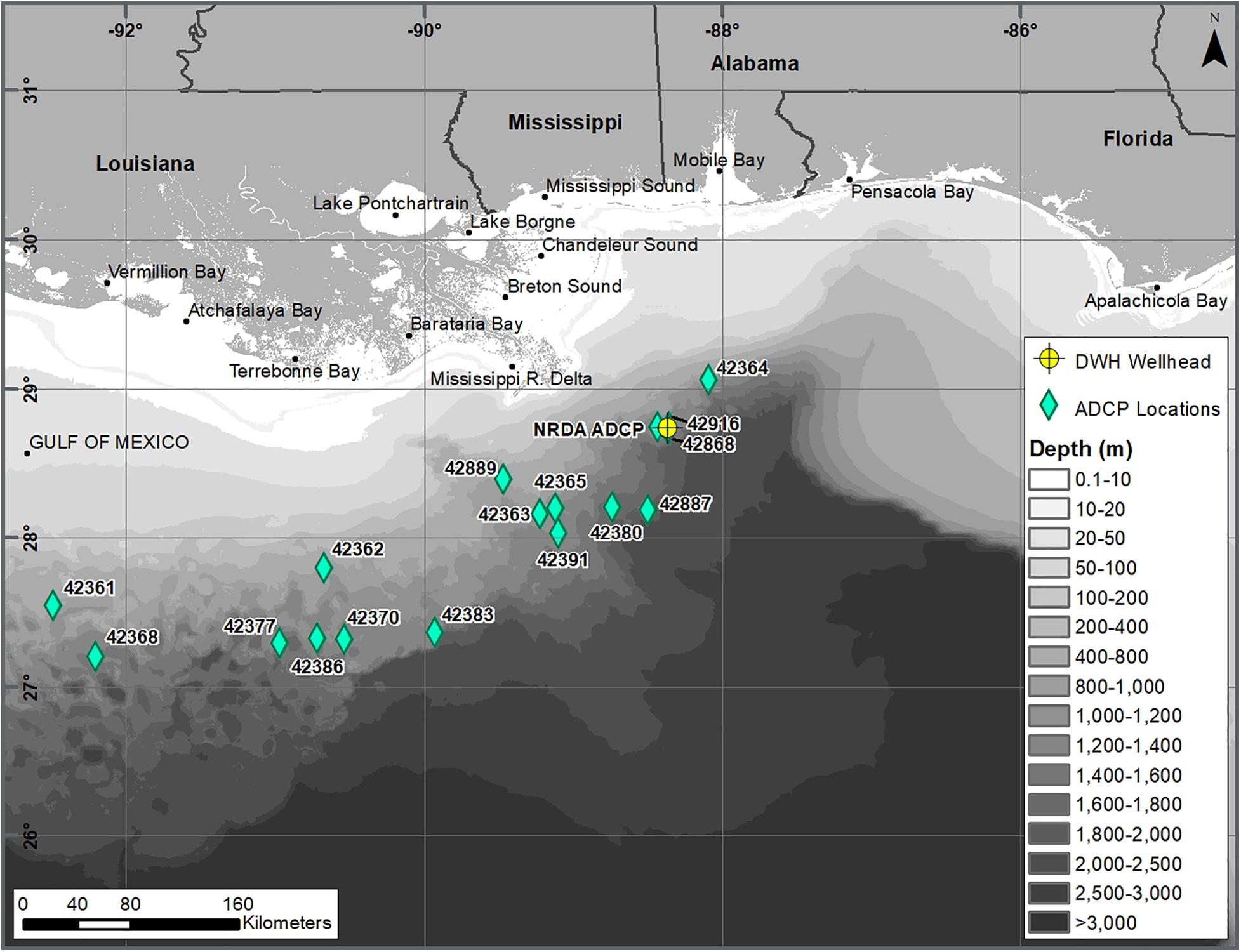
Figure 1. Map of the northern Gulf of Mexico region exposed to floating and shoreline oil from the DWH spill, showing 17 ADCP locations. (The DWH wellhead is indicated by the crossed circle. Three ADCP locations are close to the wellhead).

The ADCP data meeting quality criteria were used in SIMAP model simulations for comparison with simulations run with hydrodynamic model results. The velocity at the location of each spillet used for transport calculations at each time step was interpolated from the data taken at the 17 ADCP stations using an inverse distance-weighted scheme employing all sensors. The ADCP coverage extended along the continental slope in the area of concern, but there were no data on the shelf. In addition, the interpolation provided a smoothed current field, and did not resolve smaller scale features and shear less than the scale of the distance between ADCP moorings (order of 30–100 km). Also, ADCPs do not provide estimates of surface currents. Thus, simulations using ADCPs were realistic only for oil transport below the 40 m mixed layer in areas where ADCP data were available, i.e., over the continental slope.

Hydrodynamic models

Seven data sets of currents predicted by hydrodynamic models were evaluated. The wind data from the model used to force the hydrodynamics, along with the current data, was used in the oil spill modeling.

• HYCOM-FSU: Florida State University (FSU) performed a HYbrid Coordinate Ocean Model (HYCOM) hindcast simulation for 2010 forced with NARR winds. Data provided had 3–4 km horizontal resolution, 20 hybrid layers in the vertical, and current predictions every 3 h (Chassignet and Srinivasan, 2015).

• HYCOM-NRL Reanalysis: The United States Naval Research Laboratory’s (NRL) HYCOM + NCODA GOM 1/25° Reanalysis product GOMu0.04/expt_50.1 for 2010 forced with CFSR winds, ∼3.5 km resolution at mid-latitudes, 36 coordinate surfaces in the vertical, and current predictions every 3 h, was downloaded in March 2015⁵,⁶.

• HYCOM-NRL Real-time: The NRL Real-time operational forecast GLOBAL HYCOM (Chassignet et al., 2009) simulations for 2010 (HYCOM + NCODA GOM 1/25° Analysis GOMl0.04/expt_31.0) were forced with NOGAPS winds. Model resolution is 1/25° (∼3.5 km) in the horizontal, with 20 vertical layers, and hourly data⁷.

• SABGOM: The South Atlantic Bight and Gulf of Mexico (SABGOM) Regional Ocean Modeling System (ROMS) application was developed by North Carolina State University (NCSU) for the GOM (Hyun and He, 2010; Xue et al., 2013). The horizontal resolution is ∼5 km with 36 terrain-following vertical layers. SABGOM was forced with NARR winds. Current predictions were provided every 3 h.

• IAS ROMS: The Intra-Americas Sea Regional Ocean Modeling System (IAS ROMS) was developed from SABGOM. It was applied with a grid resolution of ∼6 km in the horizontal and 30 levels in the vertical. An IAS ROMS simulation (version “4C”) for 2010, that included a 2-km nested grid within the larger IAS ROMS domain, was run as part of the trustees’ NRDA program and provided by Chao et al. (2014) in April 2014 (model described in Chao et al., 2009). This simulation forced with NAM winds provided hourly data.

• NCOM Real Time: The Naval Oceanographic Office (NAVOCEANO) ran the three-dimensional operational global nowcast/forecast system Global NCOM through 2013. NCOM was based on the Princeton Ocean Model (POM) with time invariant hybrid (sigma over Z) vertical coordinates with 40 levels⁸. Predictions were provided every 3 h.

• NGOM: The NOAA National Ocean Service (NOAA/NOS) Coast Survey Development Laboratory (CSDL) ran the NOS GOM Nowcast/Forecast Model (NGOM), a GOM implementation of the POM, in real time during the spill, forced by NAM winds. The resolution is 5–6 km in the northeastern and central GOM, with 37 levels in the vertical. Predictions were provided every 3 h.

Geographical data

A rectilinear grid was used to designate the location of the shoreline, the water depths (bathymetry), and the habitat or shore types. NOAA Office of Response and Restoration, Environmental Sensitivity Index data⁹ were used to define shoreline habitat types, reclassifying Environmental Sensitivity Index codes to a simpler habitat classification, i.e., rocky, cobble, sand, mud, wetland, and artificial (man-made) shore types. Bathymetric data were obtained from the General Bathymetric Chart of the Oceans Digital Atlas (General Bathymetric Chart of the Oceans, 2009) one arc-minute gridded data set, which is based on quality-controlled ship depth soundings interpolated using satellite-derived gravity data as a guide.

Oil loading onto shorelines was assumed to occur up to a maximum holding capacity that was related to shore type (and so shoreline wave climate, slope, width, and grain size) and the beaching oil’s viscosity. Shore holding capacities as a function of oil viscosity were developed for each shore type based on observations from the Amoco Cadiz spill in France and the Exxon Valdez spill in Alaska, as described in French et al. (1996) and French McCay et al. (2018c).

Environmental conditions

In order to utilize the same temperature and salinity distributions for all model runs, and given the uncertainties in the subsea distributions and currents predicted by the hydrodynamic models, monthly mean water temperature and salinity data from the World Ocean Atlas (Boyer et al., 2004) were input on a three-dimensional grid. The floating oil model trajectory was not sensitive to the difference in resolution between the atlas data and the hydrodynamic model data, since most of the oil surfaced within hours of release. A synoptic map of SPM concentrations was defined for use in the oil spill modeling by combining results from field and modeling studies with satellite imagery depicting SPM plumes (French McCay et al., 2018a, c).

For the base cases, the horizontal diffusion (randomized turbulent diffusion) coefficient was assumed 100 m²/s for floating oil, 2 m²/s in surface waters (above 40 m), and 0.1 m²/s in waters below 40 m. The vertical diffusion coefficient was assumed 10 cm²/s in surface and 1–0.1 cm²/s in deep waters. The coefficients were also varied in sensitivity analyses up to one order of magnitude larger and smaller. These values are based on empirical data reviewed for the deep-water GOM (French McCay et al., 2015a; based on Okubo and Ozmidov, 1970; Okubo, 1971, Csanady, 1973; Socolofsky and Jirka, 2005, Ledwell et al., 2016).

Oil properties, composition, and degradation

The spilled oil was a light GOM crude oil. The liquid “dead” oil (i.e., oil without the C1 to C4 natural gas hydrocarbons) densities at 5, 15, and 30°C were 0.8560, 0.8483, and 0.8372 g/cm³, respectively; dynamic viscosity was 10.93 cp at 5°C, 7.145 cp at 15°C, and 4.503 cp at 30°C; and IFT was 19.63 mN/m (Stout, 2015b). Based on its asphaltene (0.27%) and resin (10.1%) content (in un-weathered dead oil, Stout, 2015b) and behavior of similar light crude oils (Fingas and Fieldhouse, 2012), the fresh oil would form an unstable emulsion. After weathering concentrated asphaltenes and resins sufficiently, the oil was observed and assumed to form a mesostable water-in-oil emulsion (mousse) up to a maximum water content of 64% water (Belore et al., 2011).

Concentrations of volatile-insoluble and soluble to semi-soluble hydrocarbons and related compounds were calculated for 18 pseudo-components used to characterize the dead oil [including nine soluble/semi-soluble and volatile/semi-volatile components defined by octanol-water partition coefficient (K_ow) range, eight insoluble and volatile/semi-volatile aliphatic components defined by boiling ranges, and one residual oil component; French McCay et al., 2015a, 2018b] and input to the SIMAP oil fates model, along with fractions of the oil volatilized in boiling cut temperature ranges (Stout, 2015a; Stout et al., 2016a). Physical-chemical properties of each pseudo-component were developed by French McCay et al. (2015a).

First-order biodegradation rates in the water column used as model input were based on reviews by French McCay et al. (2015a, 2018a,b) to develop pseudo-component-specific rates. Photo-oxidation rates of polycyclic aromatic compounds by ultraviolet light were developed by French McCay et al. (2018d).

Amounts and droplet sizes of released oil

The DWH spill location (88.367°W, 28.740°N in Mississippi Canyon Block 252, MC252; Figure 1) was ∼80 km southeast of the mouth of the Mississippi River in ∼1,500 m of water. The amount of oil (C5+) released to the environment (totaling 4.1 million bbl, ∼554 thousand metric tons, MT; i.e., not including the amount recovered at the release site) was specified from April 22, 2010 at 10:30AM CDT (local time) for 2015 hours (i.e., 84 days until July 15, 2010 at 2:30PM CDT) in 15-min time-step increments using daily estimates based on information provided by the Flow Rate Technical Group (McNutt et al., 2011, 2012), as summarized by Lehr et al. (2010). The oil mass was initialized in the SIMAP model at depths and in DSDs calculated via the nearfield and droplet size models, reflecting subsea dispersant application activities (Li et al., 2017a; Spaulding et al., 2017).

From April 28 to June 3, oil and gas flowed from both the broken end of the fallen riser and holes in a kink in the riser pipe just above the blowout preventor. After June 3 (when the fallen riser pipe section was sawed off and Top Hat #4 with a recovery pipe was placed over the riser), oil was released only from the riser pipe, around the top hat immediately above the blowout preventor. The median droplet diameters of the riser flows (∼2–3 mm) were significantly larger than those from the kink release (∼300–500 μm), due to the much higher exit velocity from the kink relative to the larger diameter riser release. For most model simulations, the best estimate of the DSD was used, which was a bimodal distribution based on partial dispersant treatment of the oil in the blowout plume (details in Spaulding et al., 2015, 2017). Sensitivity to the bounding range DSDs resulting from assumed high (100%) and low (50%) effectiveness of the subsea dispersant injections (Spaulding et al., 2015, 2017) was examined for simulations using HYCOM-FSU.

Response activities

Modeled response activities at the water surface included removal by in situ burning and dispersant application to floating oil from the air and vessels. Spatially explicit quantitative measurements of oil volume mechanically removed were not available; therefore, mechanical cleanup was not included in the model simulations. Polygons were input to the model specifying amounts of oil burned or treated by dispersant, and where and when the response activities occurred. Details are provided in French McCay et al. (2018c).

Quantitative estimates of oil volume removed by in situ burning were obtained from the Response After-Action Report by Mabile and Allen (2010; summarized by Lehr et al., 2010; Allen et al., 2011). Time ranges for burns each day were composited into a daily burn time window. The mass rate of removal on a given date was calculated as the total burn volume times typical floating oil density in the areas of the burns, 0.97 g/cm³, divided by the time range of burning that day. The model removed oil mass at this daily rate within each time and spatial window up to the maximum daily mass prescribed by the model input.

Surface dispersant application data were obtained from response records (NOAA, 2013). The volume of oil treated per dispersant volume applied (i.e., the dispersant-to-oil ratio) was based on assumptions in Lehr et al. (2010), who assumed that the minimum, median, and maximum ratios were 5, 10, and 20 by weight of oil, not including the water in mousse. The median value (1:10) was used as the base case. The fraction of oil dispersed into the water column (i.e., efficiency) was calculated using the entrainment algorithm (Li et al., 2017b) based on the assumed dispersant-to-oil ratio and resulting interfacial tension (based on data from Venkataraman et al., 2013).

Analysis of Results

To evaluate model agreement with observations, modeled floating oil distributions were compared to interpretations of remote sensing imagery, modeled shoreline oiling was compared to field survey data, and modeled subsea concentrations were compared to chemistry sample data and sensor-based indicators (e.g., fluorescence peaks).

Floating Oil

Remote sensing (satellite) imagery data were used to evaluate the distributions of surface oil over time. Remote sensing interpretations, developed as part of the trustees’ NRDA program in support of the Deepwater PDARP/PEIS (Deepwater Horizon Natural Resource Damage Assessment Trustee Council, 2016) for April to August 2010 were downloaded from the NOAA GOM ERMA website (http://gomex.erma.noaa.gov/erma.html) on January 27, 2016 (ERMA, 2016). Data from four sensors were available: Satellite Synthetic Aperture Radar (SAR), MODIS Visible, MODIS Thermal IR Sensor data (MTIR), and Landsat Thematic Mapper (TM).

Synthetic Aperture Radar images were analyzed for presence and thickness category (thick or thin) of floating oil by Deepwater Horizon Natural Resource Damage Assessment Trustee Council (2016; based on Garcia-Pineda et al., 2009, 2010, 2013a, b; Graettinger et al., 2015). MacDonald et al. (2015) used a neural network analysis of SAR images to quantify the magnitude (averaging 70 μm for thick and 1 μm for thin) and distribution of surface oil in the GOM from persistent, natural seeps and from the DWH discharge. SAR resolutions ranged from 25 to 100 m per pixel, with a few images at 6 m per pixel (Graettinger et al., 2015; ERMA, 2016).

MODIS Visible data were available for 18 days depicting surface oil, at a pixel resolution of 250 or 500 m, depending on the spectral band. The images were classified into three oil thickness classes: thin oil class (primarily silver sheen and rainbow, using NOAA, 2016), a thick oil class (transitional dark to dark color), and a moderately thick oil class (metallic sheen) that falls between the other two classes (Graettinger et al., 2015; ERMA, 2016).

MODIS Thermal IR data at a pixel resolution of 1,000 m were available for 25 days during the spill period. The images were classified into a thin oil class [primarily silver sheen and rainbow, using NOAA (2016) nomenclature], a thick oil class (transitional dark to dark color), and a moderately thick oil class that falls between the other two classes (Graettinger et al., 2015; ERMA, 2016).

Useful Landsat TM data were available over a spatially limited area on 8 days when DWH oil was on the surface of the northern GOM. Landsat TM satellite data have a pixel resolution of about 30 m. Ocean Imaging estimated the areal coverage per pixel of three oil thickness classes: a very thick class comprising heavy emulsions, a moderately thick class of dark/opaque oil, and a thin oil category that is thicker than sheen but thinner than dark/opaque oil. The Landsat TM oil thickness analyses did not classify oil sheens (Graettinger et al., 2015; ERMA, 2016).

For comparisons with model results, floating oil distributions from 84 dates and times were used, these being times where the image was judged sufficiently synoptic of the area of the floating oil. These included 34 SAR, 18 MODIS Visible, 25 MODIS Thermal IR, and 7 Landsat TM images (Supplementary Table 1). The three thickness classes of the MODIS Visible, MODIS Thermal IR, and Landsat TM images were assumed 1, 10, and 50 μm thick on average, based on ranges estimated by Graettinger et al. (2015). Graettinger et al. (2015) and MacDonald et al. (2015) aggregated the pixelated data as gridded data in a 5 × 5 km² geographic grid and developed statistical models to interpolate between observations in space and time. However, since the interpolations may have missed weather-related and other events between actual observations, comparisons of the SIMAP model results to imagery results were made using the pixelated data based on the observational data, without use of the interpolations. These non-interpolated data were gridded in the same 5 km by 5 km grid used by the Deepwater Horizon Natural Resource Damage Assessment Trustee Council (2016; Graettinger et al., 2015; ERMA, 2016).

For both the remote sensing data and the model, at each observation time for the remote sensing, the percentage of floating oil present in each grid cell was calculated in three ways.

• The relative area of oil in each grid cell indicated the distribution of oil cover. For remote sensing data, the area within the cell covered by oil was divided by the total area of oil in all cells estimated from the imagery. For the model, the area covered by spillets falling in the cell was divided by the total area covered by all floating spillets at that time step (accounting for overlapping spillet areas, avoiding double-counting).

• The estimated volume of oil in each grid cell was calculated for remote sensing data from the area covered by each thickness category. For the model, the total mass in spillets falling in the cell was used as an index of volume.

• The relative volume of oil in each grid cell accounts for the relative distribution of oil, irrespective of the actual amounts, which are subject to the assigned oil thickness. For remote sensing data, the volume of oil in each cell was divided by the total volume of oil in all cells estimated from the imagery. For the model, the total mass in spillets falling in the cell was divided by the total mass of all floating spillets in all cells at that time step. The mass was not corrected for oil density to convert to volume. Thus, all spillets were assumed to be of equal density for this index.

The Root Mean Square Error (RMSE) was calculated for each date/time there was an observation available. The RMSE is a frequently used measure of the differences between values predicted by a model and the values observed, and thus is a measure of accuracy. The individual differences (residuals) are aggregated in the RMSE as a single measure of predictive power (Fitzpatrick, 2009). For each pair of grids, the RMSE was calculated by summing the squares of the differences between modeled and the observed over all cells of the grid, where n = total number of cells in each grid:

$RMSE=\sqrt{\frac{\sum {\left(observed-modeled\right)}^2}{n}}$

RMSE values were averaged over all dates, in order to judge relative fit comparing dates and/or among simulations, the minimum RMSE indicating the best fit.

Shoreline Oil Distributions

Available data for shore oiling consisted of maps of where oil was first observed on various shoreline segments and assessments by the Shoreline Cleanup and Assessment (SCAT) program during Response. A binary discriminator test (Fitzpatrick, 2009) was used to evaluate the timing of oil coming ashore in the model, as compared with observations made by the SCAT program. The presence or absence of oil according to SCAT observations and the model predictions were gridded using the 5 km by 5 km Albers grid (ERMA, 2016) employed by the Deepwater Horizon Natural Resource Damage Assessment Trustee Council (2016) in their evaluations of oil exposure after the DWH spill. A cell was considered to have oil presence if any shore segment within the cell was observed oiled by the SCAT teams.

SCAT data were downloaded from ERMA in July of 2014 as shape files¹⁰. The observational data were binned into 10-day intervals, from April 22 to September 30, 2010. In the analysis, only those SCAT segments where oil was observed to arrive before September 30 were considered as oiled. Segments checked during the 10-day interval, but where no oil was observed to arrive, were considered as “no oil.” Segments where oil was observed to arrive after September 30, but earlier observations showed it did not arrive there before September 30, were coded as “no oil.” Note that the shorelines were not searched synoptically, and areas were not visited for days or weeks; thus, the time oil was first observed could have been a considerable time after the actual initial oiling. Also, the Deepwater Horizon Natural Resource Damage Assessment Trustee Council (2016) used additional observations and SAR to identify where oil came ashore, to develop more comprehensive maps of the locations where oil came ashore during and after (including after September 30) the spill. However, we relied solely on the SCAT survey data, as the SAR-based data were localized analyses at specific instances.

Subsea Oil

Modeled subsea concentrations were compared to chemistry sample data and sensor-based indicators (e.g., fluorescence peaks) both qualitatively, to evaluate oil locations, and quantitatively, to evaluate concentrations. We used chemical measurements of samples taken May 11 (the first date available) – July 15, 2010 and processed by the trustees’ quality-controlled NRDA program (Deepwater Horizon Natural Resource Damage Assessment Trustee Council, 2016; described in Horn et al., 2015; Payne and Driskell, 2015b, 2016, 2017, 2018; Driskell and Payne, 2018). The NRDA sample data set is available in ERMA (2016). Details of the model comparisons to subsea chemistry data are in French McCay et al. (2015a, 2018a). We summarize those findings below as part of the present analysis of the influence of physical forcing on the model trajectories and oil distributions.

Results and Discussion

The model trajectory selected as the base case for waters above 200 m was that forced with the hydrodynamic and wind input combination (i.e., HYCOM-FSU currents and NARR winds) yielding the best agreement with floating oil distributions and shoreline oiling over time. In deep water, ADCP data yielded the best agreement with oil contaminant distributions >200 m and defining the deep plume. Videos of the floating oil movements color-coded by “age” (time since release) and of the oil droplet trajectory below 900 m are in Supplementary Material.

Floating Oil

In prior modeling examining mass balance and fate of oil released from hypothetical oil and gas blowouts in nearby locations of the GOM (French McCay et al., 2018d, 2019), the initial DSD was the most influential input controlling the amount of oil surfacing. For a spill at 1,400 m, with a trap height at 1,100 m (i.e., similar to the DWH spill), a DSD with a median droplet size <700 μm reduced the amount of surfacing oil dramatically, whereas the amount of oil surfacing was similar for all DSDs with larger median droplet sizes (French McCay et al., 2019). As the breadth of (range of droplet sizes in) the DSD has been found to be narrow (Li et al., 2017a), most of the mass in the DSD is in droplet sizes close to the median droplet diameter.

In all model simulations, oil droplets >0.7 mm diameter, weathered by dissolution such that their density when they reached the surface approached 940 kg/m³ (in agreement with measurements of “fresh” floating oil by Stout et al., 2016a), rose to the surface in <17 h. Droplets 1 and 3 mm in diameter surfaced in 11 and 3 h, respectively. ADCP-measured currents at the wellhead averaged <5 cm/s between 40 and 1,400 m. Assuming a mean current of 5 cm/s during their rise, 0. 7-, 1-, and 3-mm droplets would travel ∼2, 3 and 0.5 km horizontally, respectively. Svejkovsky and Hess (2012); Svejkovsky et al. (2016) and Payne and Driskell (2015d, 2018) observed fresh oil surfacing <4 km from the wellhead on various dates in May and June 2010. Ryerson et al. (2012) observed fresh (as evidenced by measured volatiles in the air above) oil surfacing at 1.0 ± 0.5 km from the wellhead June 8–10, 2010, which based on ADCP measurements at that time implied a 10-h surfacing time. Ryerson et al. (2012) noted that visual observations from response vessels suggested a ∼3-h lag time between deliberate intervention at the well and the onset of changes in the freshly surfaced oil. These observations imply that much of the surfaced oil was comprised of droplets ∼1–3 mm in diameter. Droplets smaller than 0.7 mm rose over a longer period and so were carried progressively farther from the release point. Droplets less than ∼100 μm did not rise appreciably and formed the deep-water plume along with dissolved hydrocarbons. Thus, the DSD could affect the surfacing locations of the oil, and the floating oil distribution, depending on the relative amounts of mass in these size ranges. Floating oil would be more spread out from the well if most of the mass was in droplet sizes <700 μm than it would be if most of the mass were in droplets >700 μm.

Figure 2 shows the cumulative days of oil presence on the water surface based on SAR analysis (data from ERMA, 2016, produced by Graettinger et al., 2015). Figure 3 and Supplementary Figures 1–10 summarize the oiled footprints (north of 27°N and east of 92°W, the domain used for comparisons to focus on most of the oil and limit the number of null cells) for the model trajectories forced by various winds and currents as cumulative days of oil presence on the water surface in each grid cell over the simulation. The average RSME values over all dates of comparison for these runs, assuming the floating oil horizontal dispersion coefficient was 100 m²/s and using the modeled wind drift, are in Table 1. For the base case using HYCOM-FSU and NARR winds, and all simulations using other hydrodynamics, the DSD was the best estimate, as described in Spaulding et al. (2015, 2017). High and low cases in Table 1 represent the potential range of DSDs (Spaulding et al., 2015, 2017).

FIGURE 2

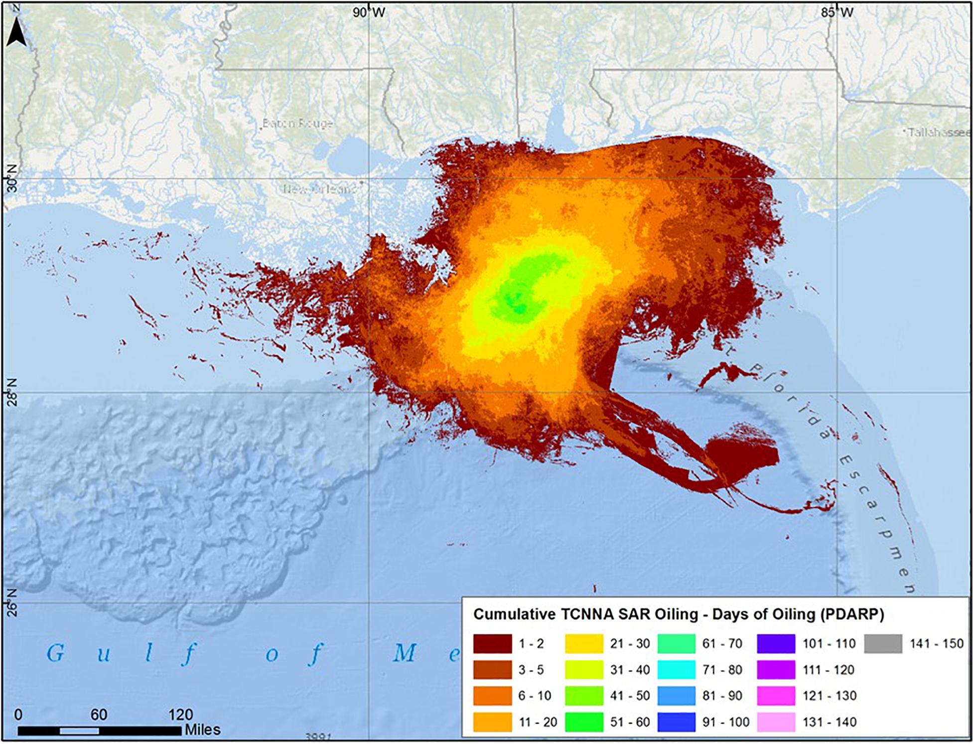
Figure 2. Cumulative days of oil presence on the water surface, based on remote sensing (SAR) analysis (data from ERMA, 2016).

FIGURE 3

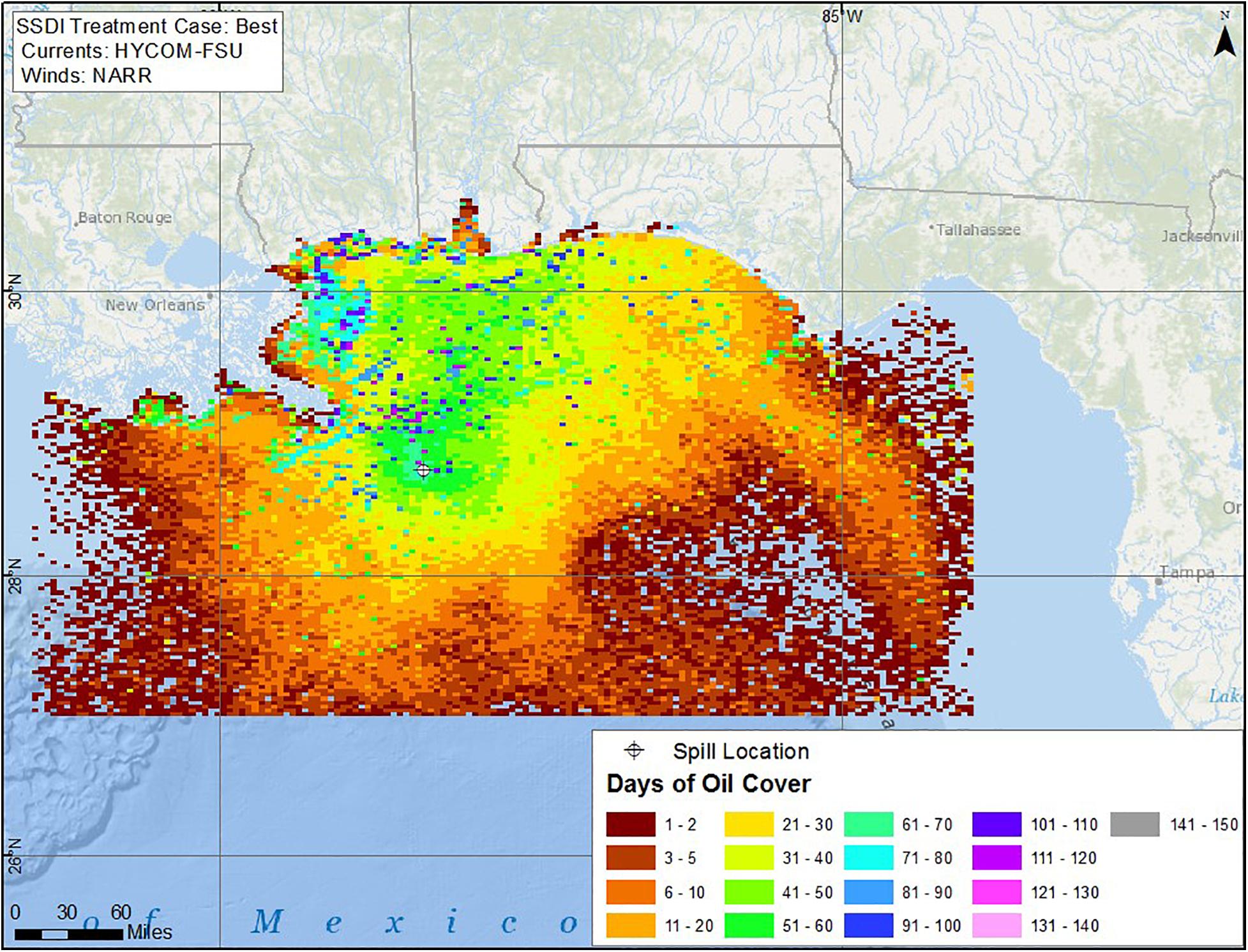
Figure 3. Cumulative days of oil presence on the water surface, based on the base case model simulation using HYCOM-FSU currents and NARR winds.

TABLE 1

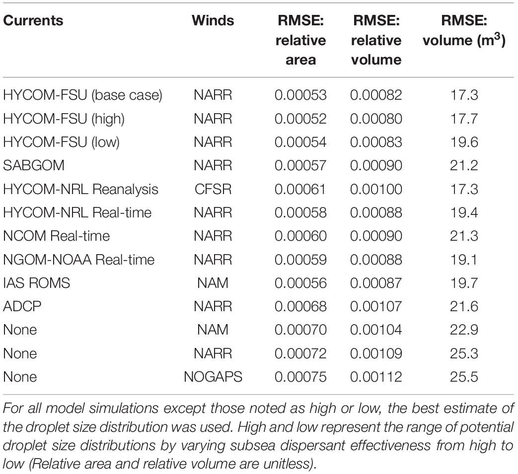
Table 1. RMSE (mean over all dates) comparing modeled to remote sensing data for floating oil distributions, varying currents and winds used as input.

Considering the RSME means for all three metrics, the base case using HYCOM-FSU with NARR winds produced a trajectory that best fit the remote sensing data. IAS ROMS showed second best agreement to the remote sensing in terms of the relative spatial distribution of floating oil (relative area and relative volume). However, the HYCOM-NRL Reanalysis with CFSR winds showed the same degree of agreement with the remote-sensing data as the HYCOM_FSU/NARR simulation in terms of oil volume distribution (Table 1). SABGOM moved more oil northeast toward Florida in June than did the other hydrodynamics (Supplementary Figure 3). The HYCOM-NRL Real-time hydrodynamics transported more oil southeast toward southern Florida (Supplementary Figure 2) than was observed in the remote sensing (Figure 2). The RMSE values show poorer agreement of the model with the remote sensing products when no currents and only winds are used, than for when any of the hydrodynamic models are used (Table 1), indicating that the hydrodynamic model currents improved the trajectories over wind drift alone. Use of ADCP data for surface transport (extrapolated from below 40 m) resulted in better agreement to the observational data than without currents, suggesting that transport of droplets rising from depth, and thus the DSD, influenced the floating oil distribution. While the mapped comparison (Supplementary Figure 7) showed the floating oil distribution reasonably agreed with the observations, there was no ADCP data on the shelf or nearshore, such that along-shore transport was not captured and there was not enough eastward or westward spread of the oil. Thus, the simulations using hydrodynamic modeled currents produced better agreement with the observed floating oil distributions than simulations using ADCP data for currents. However, as will be discussed in section “Subsea Oil,” modeled oil distributions below 40 m were in better agreement with ADCP-based observational data than simulations using any of the hydrodynamic models.

Across the range of potential subsea dispersant effectiveness assumptions (high and low cases in Table 1), the DSDs influenced the volume distribution of the floating oil to a similar degree as varying the hydrodynamic model input. However, the relative area and relative volume RMSE values did not change much with change in DSD within the potential range (Spaulding et al., 2015, 2017), whereas those metrics were sensitive to the hydrodynamic input. The best-estimate DSD used for the base case with HYCOM-FSU yielded the lowest RMSEs overall (Table 1). Thus, the floating oil spatial and volume distributions were sensitive to the hydrodynamics used. The relative spatial distribution of the floating oil was not sensitive to the plausible DSD inputs because the substantial mass in large droplets (>0.7 mm) surfaced close to the well and resulted in similar trajectories, regardless of the amount in those droplet sizes. If the DSD were skewed to much smaller sizes than those examined, the relative spatial distribution would be affected, and floating oil would be more broadly distributed since smaller droplets would be carried farther from the well before surfacing. However, such DSDs are not realistic for the DWH spill where the conditions and dispersant volumes applied at depth were not conducive to creating smaller droplet sizes (Adams et al., 2013; Zhao et al., 2014, 2015; Socolofsky et al., 2015b; Spaulding et al., 2015, 2017; Nissanka and Yapa, 2016; Testa et al., 2016; Gros et al., 2017; Li et al., 2017a; Daae et al., 2018; National Academies of Sciences Engineering and Medicine, 2020). The extremely low estimates of the median (<100 μm) and maximum (<300 μm) droplet diameters (for both untreated and treated oil) of Paris et al. (2012) and Aman et al. (2015) were not representative of the DWH conditions (see Adams et al., 2013; Testa et al., 2016), nor are they consistent with the field evidence.

As SIMAP is a Lagrangian model, the diffusion coefficients moved the spillet centers randomly each time step at a scale determined by the coefficient. Those displacement distances were small relative to the ∼5-km concentration grid used to compare the model to the remote sensing data. Thus, the RMSE values changed slightly (<10%) with differing floating oil horizontal dispersion coefficients from 5 to 200 m²/s, indicating this assumption had little influence on the results at the scale of a 5 km grid. The hydrodynamic models did not resolve the surface oil drift in the upper wave-mixed layer resulting from wave motions and Ekman flow. Simulations using the Youssef and Spaulding (1993) model of these processes, as well as varying percentages-of-wind-speed drift rates (2–4%) and angles (0–20°) to the right of downwind, showed that the best fit was consistently that using the Youssef and Spaulding (1993, 1994) model, as opposed to using a constant wind drift percentage and angle for all dates, although the differences between the results were small on most days (results not shown). Moreover, there was much more variation between runs with different currents and winds used for forcing than the differences due to variation in wind drift model or the horizontal dispersion coefficient. Thus, variations of wind drift and horizontal dispersion coefficient assumptions were not examined further. Use of 800,000 spillets instead of 100,000 spillets (as used for the simulations presented) to represent the floating oil slightly improved the model agreement with the observed for the HYCOM-FSU base case, as the additional spillets filled in some of the areas where remote sensing data indicated oil was present. However, model run time was increased considerably in the tests using more spillets.

Snapshots of surface oil distributions over time, predicted by the model using HYCOM-FSU currents and based on remote sensing data, are compared in the Supplementary Material. Comparative snapshots for other model simulations are available in French McCay et al. (2018c). Figure 3 and Supplementary Figures 1–10 summarize the trajectories and comparisons. The remote sensing data indicate the floating oil was primarily in a circular area near and just north of the DWH wellhead. The simulations using HYCOM-FSU (Figure 3), HYCOM-NRL Reanalysis (Supplementary Figure 1), and IAS ROMS (Supplementary Figure 6) show similar patterns. The results of the simulations with other currents show excursions too far northeast (SABGOM, Supplementary Figure 3; NCOM Real-time, Supplementary Figure 4), and too much dispersion in all directions (HYCOM-NRL Real-time, Supplementary Figure 2; NGOM, Supplementary Figure 5). The three simulations using no currents and NAM, NARR or NOGAPS winds (Supplementary Figures 8–10) are similar, and do not transport of the floating oil enough to the east or west. Otherwise, the no-current simulations result in realistic floating oil patterns centered just north of the wellhead. The simulation using ADCP currents and NARR winds generates results similar to no currents and NARR winds (Supplementary Figure 7), because the ADCP currents are relatively weak in the offshore area and do not cover the shelf or nearshore. These results indicate the importance of the wind drift in transporting the floating oil, but that the currents used can change the patterns dramatically.

The modeled number of days of oil cover for the base case using HYCOM-FSU (Figure 3) is of the same range as the SAR-based estimates (Figure 2) in the area of the wellhead and off the Mississippi River Delta. However, the duration of oil cover in the area near the coast of Mississippi and Alabama is higher in the model than the SAR data indicate. Also, floating oil trapped near shore in the model remained longer than observed. Mechanical removal, on water or on shorelines, was not included in the simulations, and this could potentially account for at least some of the observed reduction in the nearshore floating oil.

The RMSE values for the base case using HYCOM-FSU currents (Figure 4) show the best agreement in terms of relative area or relative volume distribution in early June, whereas the model estimated volume of oil was most similar to the remote-sensing based estimates in April-early May and in July. The results for other current-wind combinations showed similar temporal patterns. The relatively high RMSE values for spatial coverage in April were because the modeled distribution remained more localized around the wellhead than the remote sensing indicated. The relatively high RMSE value for relative volume on May 17 was for the MODIS visual image of that date, when the “Tiger Tail” feature (i.e., the extension to the southeast as oil sheen was drawn into a cyclonic eddy) was seen in the imagery (Walker et al., 2011; Olascoaga and Haller, 2012) but not indicated by the model (i.e., the hydrodynamic model did not locate the eddy in the same location at that time).

FIGURE 4

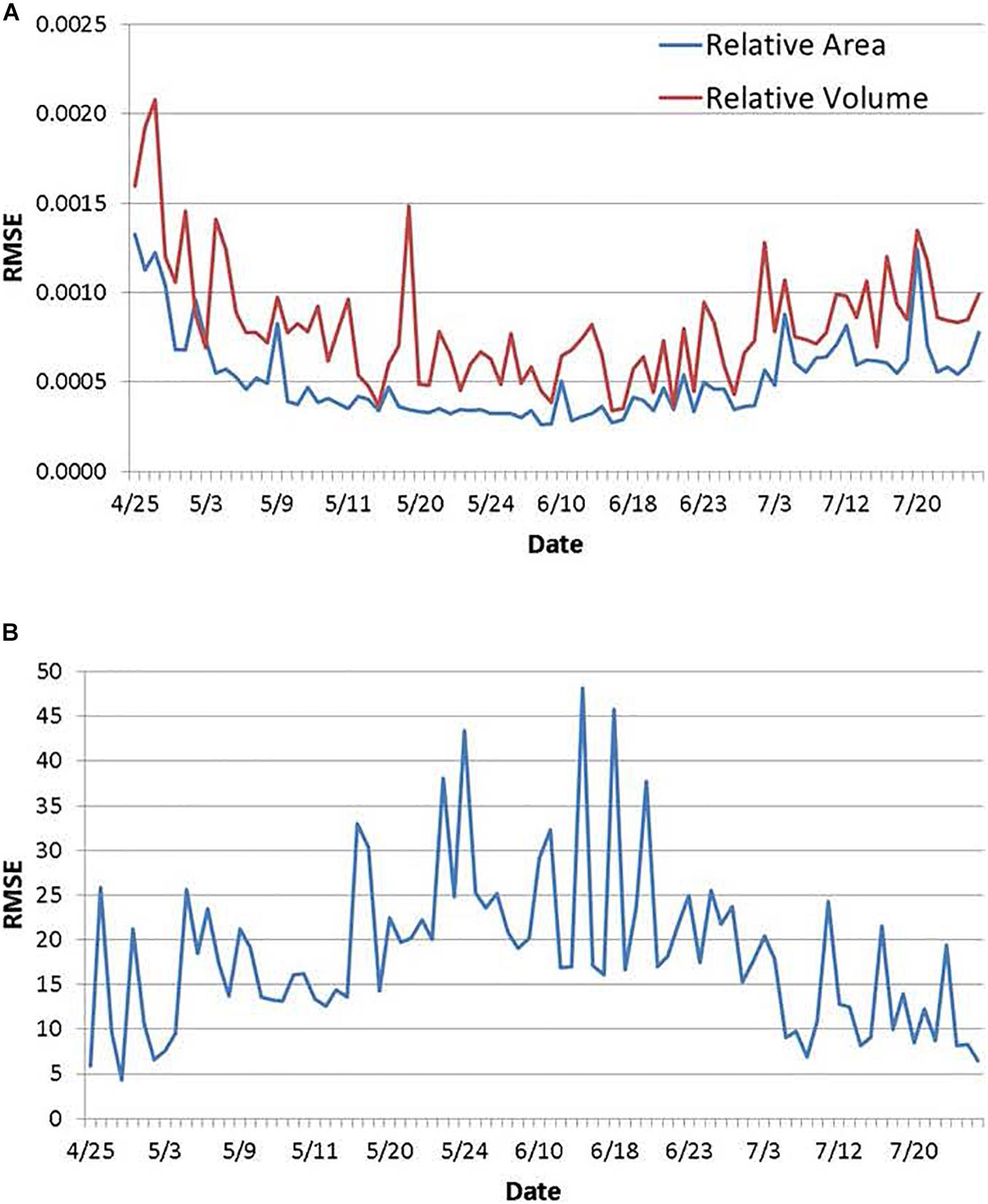
Figure 4. RMSE of relative area and volume (as fractions, panel A) and of oil volume (m³, panel B) for the base case model simulation (using HYCOM-FSU) compared to remote sensing-based data.

The modeled maximum amount of oil in each grid cell at any time in the simulation is shown in Figure 5. Using gridding with a cell size of 25 km², MacDonald et al. (2015) estimated the footprint of aggregated floating oil and oil emulsions, where oil coverage exceeded ∼1 g/m² at some time during the spill, which extended over 149,000 km². By comparison, the base case model prediction, using the same resolution and threshold, was 194,000 km². The model predictions included some low concentrations of floating oil in areas far from the well where oil was not detected by the remote sensing. These small patches of highly weathered oil residuals (>20 days old) in the outskirts (see the video of the floating oil movements color-coded by age in Supplementary Material) were likely undetected in the remote sensing analyses because of the resolution of those sensors. The modeled time-averaged mean oil cover (Figure 6) is similar in pattern and of the same magnitudes as the estimates made by MacDonald et al. (2015) based on SAR analysis. Their estimated daily average footprint was 11,200 km² (SD = 8,430 km²). The model estimate (base case) of the daily average surface area affected by floating oil >1.0 g/m² was 6,720 km² (SD = 4,960 km²), not significantly different from the remote sensing daily estimate.

FIGURE 5

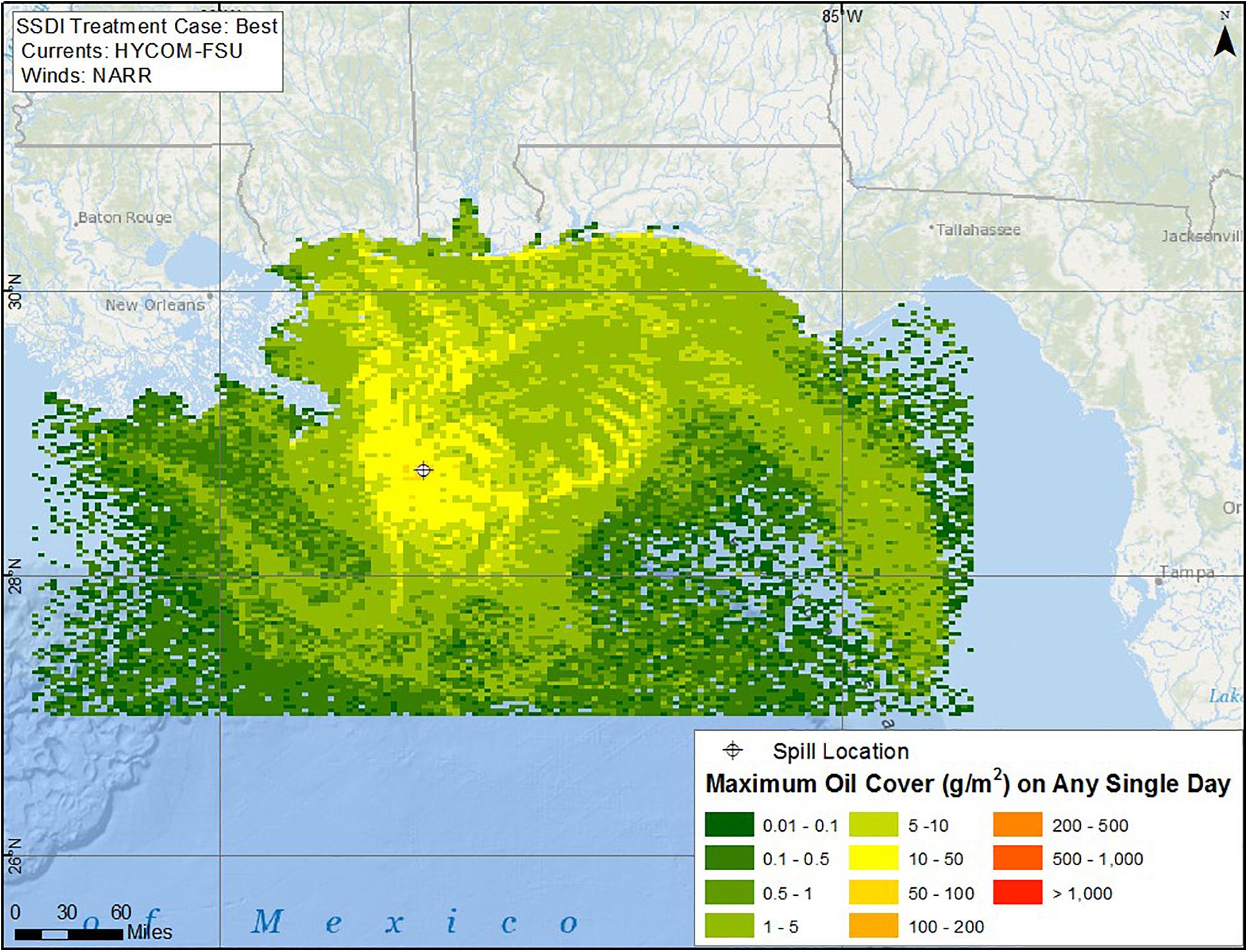
Figure 5. Modeled maximum amount of oil in each grid cell at any time in the simulation (as g/m² averaged over the grid cell), based on the base case model simulation.

FIGURE 6

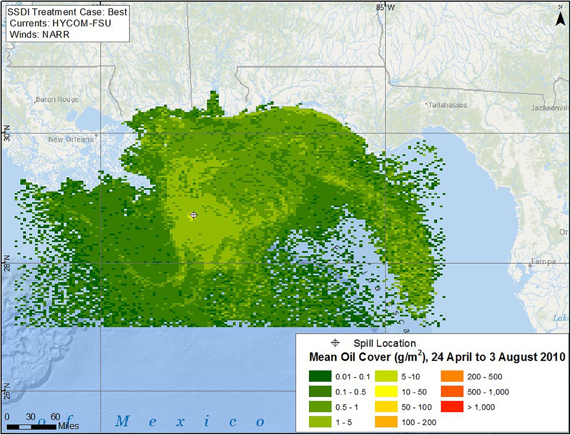
Figure 6. Time-averaged mean floating oil concentration (g/m²) in each cell for the period when oil was observed by SAR, 24 April to 3 August 2010, based on the base case model simulation.

Note that the gridded summaries of floating oil distributions, both for the model and for the remote sensing data, provided average amounts of oil mass over the cell area. They should not be interpreted as an actual oil thickness, as the oil is patchy and of varying thicknesses within the cells. The remote sensing data are typically expressed as volumes per cell for this reason. Furthermore, the total area of the cells where oil is present is larger than the actual oil coverage at any given time. The modeled areas covered by oil, the sum of the areas covered by spillets (representing patches) at a single time step, were an order of magnitude lower than those estimated from the gridding. The mean swept area from April 24 to August 3, 2010 (101 days) was 1,960 km²/day for the model base case.

The modeled amount of floating oil for the base case simulation is compared to remote-sensing based estimates in Figure 7. The modeled floating oil volumes, and to some degree the remote-sensing-based estimates, are inversely related to wind speed, as wind events entrain oil into the water and oil accumulates on the water surface during calm periods. While there is considerable variability in the remote-sensing based estimates, in large part due to uncertainty in the oil thickness estimates (Graettinger et al., 2015) used, the model predictions over time are within the range of the remote-sensing estimates. From May 1 to July 31, 2010, the modeled floating oil volumes averaged 27,100 m³ (26,500 MT), whereas the remote-sensing based estimates averaged 25,900 m³. The average floating oil volumes were 27,700 m³ (27,200 MT) and 29,400 m³ (28,800 MT) for the high and low effectiveness cases, respectively. With no subsea dispersant use, the model predicted an average of 29,800 m³ (29,200 MT) of floating oil in May–July 2010.

FIGURE 7

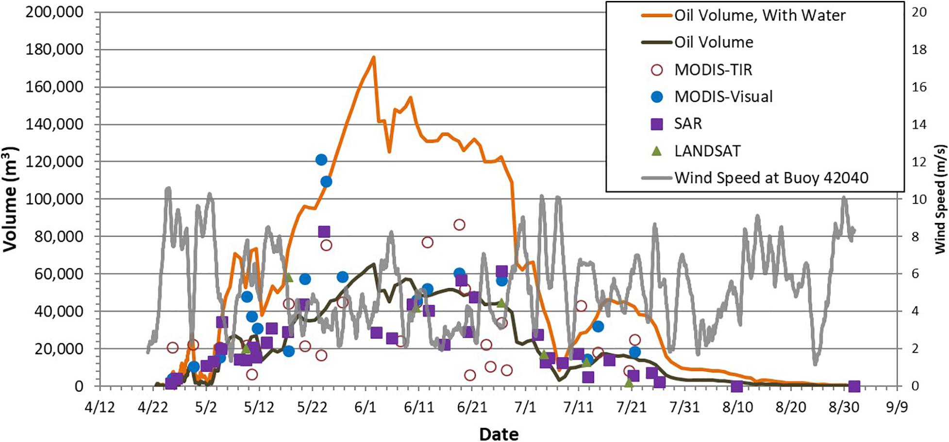
Figure 7. Volume of surface floating oil, including the oil only or with the water in emulsions, for the base case model and calculated from remote sensing data; wind speeds at NOAA buoy 42040.

Shoreline Oil Distributions

Approximately 2,100 km of beaches and coastal wetlands were exposed to MC252 oil in 2010, according to the Deepwater Horizon Natural Resource Damage Assessment Trustee Council (2016; Nixon et al., 2016). The oil was documented by shoreline assessment teams as stranding on 1,773 km of shoreline. Deepwater Horizon Natural Resource Damage Assessment Trustee Council (2016) mapped maximum observed oiling, categorized as not surveyed, no oil seen, or various degrees of oiling. Many areas were not surveyed, including much of Mobile Bay and considerable areas of wetlands in Louisiana. Thus, the 2,100 km estimate likely underestimates the actual length of shoreline affected by oil.

Modeled shoreline oiling results are summarized in Table 2. For simulations run without currents, the length of shoreline oiled is smaller and focused on the area between the Mississippi River Delta and Alabama. The total length of shore oiled estimated by the Deepwater Horizon Natural Resource Damage Assessment Trustee Council (2016; Nixon et al., 2016) was 2,113 km. The categories of degree of oiling used by the Trustees cannot be translated to oil loading amounts (g/m²). The total lengths of shoreline oiling predicted by the model using most of the hydrodynamic model currents (except NGOM) are 2,000–2,700 km oiled, with the base case predicting 2,568 km oiled. These results are in good agreement with the observations, considering some areas were not surveyed.

TABLE 2

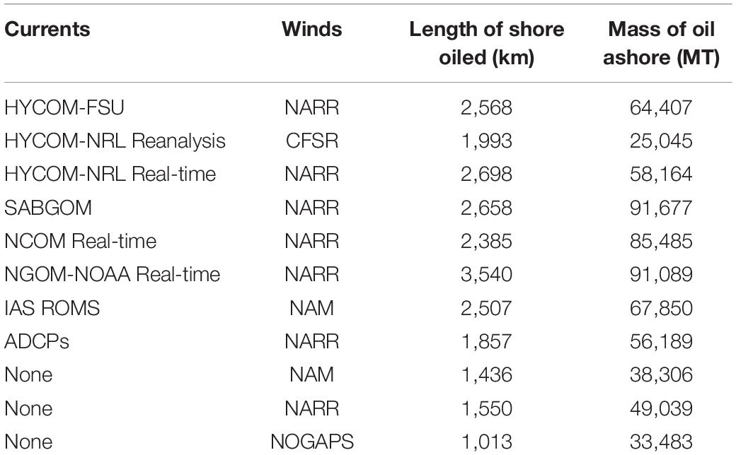
Table 2. Shoreline oiling results for model cases, varying currents and winds used as input.

Figure 8 and Supplementary Figures 11–16 summarize the comparisons of the modeled shoreline oiling with SCAT-based observations, showing the variability resulting from different current and wind inputs. These maps color code where oil came ashore in the model but where the shoreline had not been surveyed (“no observed coverage, modeled oil”), as well as where both modeled and observed indicate oil (“match”), where both observed and the model indicate no oil (“no observed oil”), where there are false negatives (observed only), and where there are false positives (modeled only).

FIGURE 8

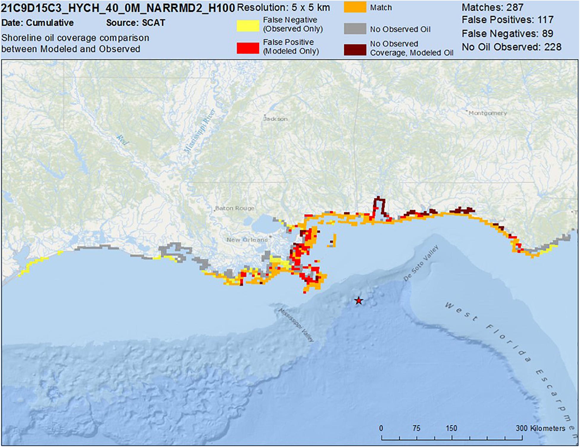
Figure 8. Comparison of model predictions, for the base case simulation using HYCOM-FSU Reanalysis currents and NARR winds, to SCAT-based observations of cumulative amount of oil coming ashore by September 30, 2010.

The modeled shoreline oiling for the base case compares well with the observations (Figure 8), the model showing oiling from the Apalachicola Bay area of Florida to Terrebonne Bay area of Louisiana. Note that the model predicted shore oiling inside Mobile Bay in areas where it was not observed. However, as most of Mobile Bay’s shoreline areas were not surveyed, oiling of those areas is unknown. No oil was reported in some of the small bays along the Florida panhandle. However, booming may have prevented oil from entering those inlets, whereas booming was not included in these model simulations.

Simulations using HYCOM-NRL Reanalysis currents with CFSR winds (Supplementary Figure 11), HYCOM-NRL Real-time currents with NARR winds (Supplementary Figure 12), and NCOM Real-time with NARR winds (Supplementary Figure 14), predict similar oiling patterns to the base case using HYCOM-FSU currents and NARR winds (Figure 8). SABGOM spreads oil to shorelines too far to the east and into western Louisiana where no oiling was observed (Supplementary Figure 13). NGOM currents with NARR winds and the IAS ROMS simulations carry too much oil to western Louisiana and Texas but otherwise show good agreement with the SCAT observations (Supplementary Figures 15, 16). Simulations made with no currents, forced with winds only, and those forced with ADCP currents and NARR winds, do not bring as much oil ashore west of the Mississippi River Delta as was observed. Thus, coastal currents prevailing toward the west apparently transported the oil to those areas. Also, currents brought the oil east to Florida, as winds alone do not account for that shoreline oiling.

The shoreline oil distributions were more accurate when westward flows near the Mississippi Delta were simulated in the forcing hydrodynamic model. Novelli et al. (2020) identified westward flows as due to easterly winds. Kourafalou and Androulidakis (2013); Androulidakis and Kourafalou (2013), and Androulidakis et al. (2015, 2018) examined and stressed the importance of the Mississippi outflow in controlling nearshore oil movements and shoreline oiling distributions. The HYCOM models seemed to have captured these dynamics reasonably well in simulating conditions in the summer of 2010, whereas the ROMS implementations examined did not reflect those dynamics. It is possible that Mobile Bay was protected by freshwater outflows not captured in any of the hydrodynamic models. However, oiling data in Mobile Bay were insufficient to determine how much entered the bay.

Weisberg et al. (2017) concluded that the general circulation from the hydrodynamics modeling could account for transporting the Deepwater Horizon oil to near shore, but that the waves, via Stokes drift, were responsible for the actual beaching of the oil. In our analysis, we found the wind drift (i.e., including Ekman flow and Stokes drift) was the primary driver for bringing oil to shore. Le Heìnaff et al. (2012) and Boufadel et al. (2014) also concluded that wind drift was the most important factor bringing oil ashore. Using several hydrodynamic models as input, Boufadel et al. (2014) concluded that the wind drift rate was 1–4% of wind speed. Studies by Novelli et al. (2020) found that along-shore easterly winds followed by southerly wave-induced surface drift brought drifters, and so the DWH oil, ashore. Conversely, westerly winds moved the surface water and drifters away from shore. However, to the degree that the circulation modeling includes the wind-forced circulation, the relative importance of what is considered due to hydrodynamic inputs versus “wind drift” would vary. Dietrich et al. (2012) performed a detailed analysis comparing modeled oil drift using hydrodynamic and wave models as compared to satellite imagery, finding the best agreement using their implementations of Simulating WAves Nearshore (SWAN) and ADvanced CIRCulation (ADCIRC) models as the sole forcing. The inclusion of wind drift on top of the hydrodynamic and wave models transported the oil too fast. Thus, careful consideration is needed to determine the degree to which wind drift should be applied in the oil spill model, depending on the forcing and resolution included in the hydrodynamics and wave models.

Figure 9 maps the modeled shoreline oiling for the base case using HYCOM-FSU, along with modeled concentrations of sedimented oil by August 31, 2010 (Sedimentation is discussed below). Maps of the results for the base case simulation for each of the 16 10-day intervals from April 22 to September 30 are available in French McCay et al. (2018c). No oil came ashore in the first 10-day period, April 22–May 1, in either the model or SCAT observations. The oil’s arrival to shore was in good agreement with the SCAT observations for most areas and observation periods. The exception was that the (base case) model did not bring as much oil ashore west of the Mississippi River Delta during early to mid-June as was observed. Oil did come ashore in that simulation later in June and in July.

FIGURE 9

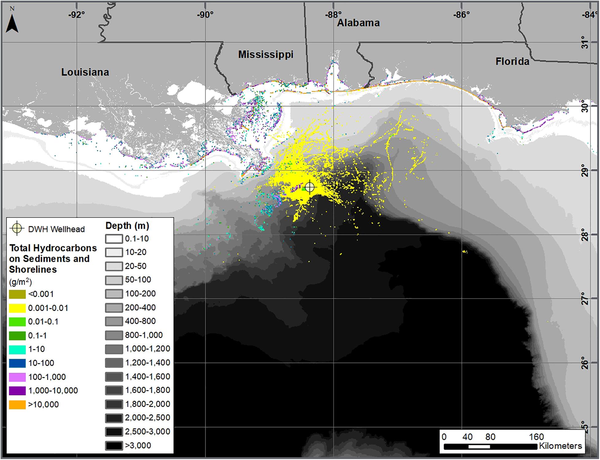
Figure 9. Cumulative amount of oil coming ashore and settling to sediments (in g/m²) by August 31, 2010 for the base case simulation using HYCOM-FSU currents and NARR winds.

Subsea Oil

Comparisons of modeled subsea oil component concentrations to field chemistry samples are described in French McCay et al. (2018a). Here we summarize those findings and evaluate the modeled movements of the oil below 200 m using various current data as input.

Camilli et al. (2010) detected the deep plume at ∼1,000–1,200 m during June 23–27, 2010. Their Sentry’s methane m/z signal at 35 km from the source was only 53% less than that at 5.8 km, suggesting that plume extended considerably beyond the 35 km survey bound at that time. The model using ADCP data simulated the plume as extending to the southwest 60 km on June 23 and 82 km on June 27 (video of spillet movements below 900 m in Supplementary Material), consistent with the observations by Camilli et al. (2010).

While the oil-affected volume has been described as an inverted cone over the well with large droplets rising in the center and progressively smaller ones further from the well (e.g., Ryerson et al., 2012; Spier et al., 2013), due to ADCP-documented current shear and varying rise rates for different diameter droplets, “plumes” of rising oil droplets followed different trajectories during their ascent toward the surface, a behavior captured in our model simulations (French McCay et al., 2018a, c). In addition, while rising, the intermediate-sized droplets lost some of their relative buoyancy due to weathering (dissolution and biodegradation), as well as potentially combining with SPM in the water column. The ambient current higher in the water column is increasingly stronger than in deep water (Hyun and He, 2010), such that the intermediate sized droplets would have separated to form “multiple plumes” of slowly rising droplets in the upper layers mimicking the deep water plume. Fluorescence anomalies (peaks) and water column hydrocarbon chemistry data (Camilli et al., 2010; Valentine et al., 2010; Spier et al., 2013; as well as NRDA data, Horn et al., 2015 and Payne and Driskell, 2015a,c, 2018) showed relatively high concentrations in finite “clouds” of particulate- and dissolved-phase oil at various depths above the intrusion at ∼1,100–1,200 m. The SIMAP model simulated these behaviors and distribution. Sensitivity analyses by North et al. (2011, 2015) and Paris et al. (2012) showed similar behavior: droplets with diameters of <50 μm formed distinct subsurface plumes that were transported horizontally and remained in the subsurface for >1 month; while droplets with diameters ≥90 μm rose to the surface, more rapidly at larger diameters.

Fluorescence peaks (relative high values) and dissolved oxygen “sags” (relatively low values) in vertical profiles associated with elevated hydrocarbon concentrations in water samples were consistently observed at depths ∼1,000–1,300 m mainly southwest of the wellhead (Joint Analysis Group, 2010; French McCay et al., 2015a, 2018a; Horn et al., 2015). In the deep plume, the ADCP-measured speeds averaged 3.9 cm/s to the southwest. Measured current speeds were consistently <10 cm/s at all depths and for most of the period of the oil release. ADCP data in ∼30–60 m vertical bins throughout the upper ∼1,000 m of the water column showed currents in adjacent depths differing by as much as 120° in direction during May–June 2010 (French McCay et al., 2015a, 2018a).

In contrast, in the area of the DWH wellhead, all of the hydrodynamic models examined (three HYCOMs: HYCOM_FSU, HYCOM-NRL Reanalysis, HYCOM-NRL Real-time; two ROMS: SABGOM, IAS ROMS; and two POMs: NCOM Real-time, NGOM) calculated much higher speeds for the currents in the deep plume and water column below 200 m than is indicated by the ADCPs. Furthermore, the movements were less consistently toward the southwest than indicated by the ADCP and field observation data. This was evident in trajectories of oil droplets below 200 m. The video of the oil droplet trajectory below 900 m using ADCP data in the Supplementary Material summarizes the movements of oil in the deep plume. Snapshots in the deep plume and at intermediate depths from trajectories using the hydrodynamic models are available in French McCay et al. (2018a, c).

The hydrodynamic models produced current fields below 200 m that at times agreed with the ADCP data, and in other times diverged in direction and speed. The HYCOM-FSU model produced a trajectory of small droplets in deep water (French McCay et al., 2018a, c) that was most similar to that using the ADCP data (video of the oil droplet trajectory below 900 m using ADCP data in Supplementary Material). The ROMs models tended to transport the small droplets along the bathymetry toward the southwest in narrow smooth flows much faster than indicated by the ADCP data. The IAS ROMS simulation (described in French McCay et al., 2015a, 2016) was very similar to the SABGOM simulation (in French McCay et al., 2018a, c). The HYCOM-NRL Real-time and HYCOM-NRL Reanalysis both predicted the deep plume moved primarily northeastward from April through July of 2010, such that the modeled deep plume did not extend southwestward in July as observed (French McCay et al., 2018c). The POM models (NGOM is shown in French McCay et al., 2018a) predicted movements at times to the northeast and other times to the southwest, but the timing of movements in these directions did not agree with the ADCP and observational data. The NRL NCOM model was superseded by NRL’s HYCOM, which produced more realistic (slower) currents at depth, and so the NCOM simulations were not considered further.

Given the more narrow and accurate surfacing locations (see section “Floating Oil”), the simulation using ADCPs was the most realistic for depths below 200 m. While the interpolation of the ADCP data was not a hydrodynamic model, which conserved mass and momentum, the ADCP current data does indicate the actual flow field and which of the hydrodynamic models most closely simulated it (i.e., the HYCOM-FSU model).

In the SIMAP model simulations using the ADCP data and using HYCOM-FSU, the concentrations of droplets and dissolved constituents were highest close to the source (i.e., ∼1,200 or ∼1,300 m). Because the smaller oil droplets were spread out by spatially and time-varying currents as they rose through the water column, the modeled concentrations decreased considerably higher in the water column. Oil concentrations in the deep water were low and in a narrow cylinder stretching toward the surface in April, when the release was not treated with dispersants at the release point and the oil was mostly in the form of large droplets >0.7 mm in diameter. During May when the kink holes appeared and subsea dispersant began to be applied, such that small droplets were formed in addition to droplets >0.7 mm in diameter (Spaulding et al., 2015, 2017), the modeled subsurface concentrations were much higher, and the contamination was dispersed over a wider area. As shown by the sample data (Horn et al., 2015; Payne and Driskell, 2018), the deep plume of small droplets and dissolved components persisted from May to July. The model results show more extensive plumes in deep water in June–July when more effective subsea dispersant applications were used than prior to June 3. See French McCay et al. (2015a, 2016, 2018a,c) for further detail and maps depicting the concentration distributions in space and time.

Oil Sedimentation

Oil from the DWH spill was identified in the sediments in the offshore area surrounding and down-stream of the well site (Joye et al., 2011; Montagna et al., 2013; Valentine et al., 2014; Romero et al., 2015; Stout and Payne, 2016a; Stout et al., 2016b). Valentine et al. (2014) noted that the pattern of contamination indicates deep-ocean intrusion layers as the source, consistent with deposition of a “bathtub ring” formed from an oil-rich layer of water impinging laterally upon the continental slope (at a depth of ∼900–1,300 m) and a higher-flux “fallout plume” where oil-SPM aggregates sank to underlying sediment (at a depth of ∼1,300–1,700 m).

Figure 9 maps the modeled sedimentation by August 31, 2010 for the base case using HYCOM-FSU for surface waters and ADCP data in deep water. The modeled sedimentation in deep water due to fallout by interactions with SPM and the bathtub ring impingement was in consistent locations to those mapped by Valentine et al. (2014), Stout et al. (2016a), and Romero et al. (2015). The model also predicted considerable sedimentation in the nearshore waters of Louisiana.

Conclusion

Summary of Findings

The modeled spatial distribution of surface oil was validated by comparison to remote sensing data. As the model ran continuously from April 22 through September of 2010, disagreement would be expected for older oil. However, freshly surfacing oil reset the modeled origin of the slicks on a continuous basis. The results indicate the importance of the wind drift in transporting the floating oil northward toward shore (consistent with Dietrich et al., 2012; Le Heìnaff et al., 2012; Boufadel et al., 2014; Weisberg et al., 2017), but that the currents used can change the patterns considerably. The model-predicted amount of floating oil agreed with remote-sensing based estimates, confirming the modeled DSDs and fate processes were realistic.

The modeled shoreline oiling for the base case (∼2,600 km oiled) compares well with the observations (∼2,100 km oiled; Nixon et al., 2016), with the model showing oiling from the Apalachicola Bay to Terrebonne Bay. The model predicted oiling on shore in areas that were not surveyed, so oiling of those areas based on observations is unknown. Other model simulations demonstrated the variability resulting from different current and wind inputs. Shoreline oiling events were discontinuous and occurred when winds (via wind drift) carried oil onshore.

Simulations of subsurface oil movements using current data from seven hydrodynamic models resulted in very different trajectories, and to varying degrees the hydrodynamic models generally over-estimated the speed of the currents in the area of the wellhead. Published DWH oil trajectory simulations (MacFadyen et al., 2011; Mariano et al., 2011; North et al., 2011, 2015; Dietrich et al., 2012; Le Heìnaff et al., 2012; Paris et al., 2012; Boufadel et al., 2014; Lindo-Atichati et al., 2014; Testa et al., 2016; Weisberg et al., 2017) show highly variable paths and concentrations as well. MacFadyen et al. (2011); Mariano et al. (2011), Le Heìnaff et al. (2012); Dietrich et al. (2012), Boufadel et al. (2014), and Weisberg et al. (2017) compared their predicted surface oil movements to field data, finding wind drift to be important to transport, along with the hydrodynamic model produced currents. However, they did not analyze subsea movements of the oil in comparison to observations. In our modeling studies, the base case simulation using currents generated by the HYCOM-FSU hydrodynamics model (Chassignet and Srinivasan, 2015) consistently resulted in both a subsea trajectory and concentration fields most similar to that predicted by the ADCP measurement-based current field below 200 m. The flow was generally toward the southwest, as the ADCPs indicated occurred (French McCay et al., 2018a). The HYCOM used by Paris et al. (2012), which was apparently the same HYCOM-NRL Real-time product we used, also showed similar movements of small droplets in the deep plume.

Because most of oil forming the surface slicks was from large droplets that surfaced near well, it was not very displaced by deep currents. Thus, use of the various hydrodynamic models for transport below 200 m did not greatly influence the surfacing locations to the point where it would be perceptible in the overall distribution of floating oil (i.e., as compared to synoptic remote-sensing based maps of oil distributions). Thus, the modeling problem can be treated in two domains: waters below 200 m in the offshore and surface waters above 200 m both offshore and over the shelf to nearshore.

Implications for Modeling Environmental Exposures

This modeling effort is unique and ground-breaking in several ways. The objective is to quantify by modeling oil transport, fate, exposure concentrations, and (as part of follow-on studies) biological effects (French McCay et al., 2015a,b,c,d,e being the first syntheses of these efforts). Thus, the modeling predicted oil transport, fate and exposures continuously over the entire spill period, including in deep water and surface waters. Transport modeling evaluated nine potential hydrodynamic inputs (seven models, measurement data and an assumption of no currents). The complexities of the oil composition and weathering were tracked using pseudo-components, such that exposure concentrations could be characterized by concentrations of each pseudo-component in the mixtures. Most fate processes were quantified as well, as opposed to evaluating implications of certain assumed inputs, such as droplet size or biodegradation rates. However, some fate processes could not be quantified for lack of sufficient information, such as related to marine oil snow formation and its flux to the sea floor. The exposure modeling (French McCay et al., 2015b,c) involved distribution, behavioral analysis and simulation of movements of many biological groups and life stages, recording their exposure histories to oil components, the results of which are being analyzed. We have also made a concerted effort to validate the model simulations at each stage of the overall effort. Such a comprehensive modeling and validation exercise has not been attempted previously.

The importance of data assimilation is well-established for calibrating physical models with observational information, and the tested and literature-reported hydrodynamic models do include assimilation of such information as sea surface height and temperature. However, data assimilation techniques have not been applied in oil spill models. Rather, many of the literature-reported oil trajectory model exercises (such as some of those noted above) ran short-term trajectories from known oil positions, as opposed to long simulations where displacement errors would compound. MacFadyen et al. (2011) described their approach for modeling during the response period where trajectories were reinitialized from identified remote sensing-based observations, and different hydrodynamic models were used over time, in order to obtain the more accurate trajectories.

While such a nudging-based initialization approach was considered and tested, whereby oil positions were updated with remote sensing observations, as was done for the response modeling (MacFadyen et al., 2011), this led to discontinuities in the concentrations of oil on the surface and in the water column beneath it. Thus, the exposures to biota were not reflective of reality and under-estimated when oil was repositioned. Further, weathering history of each oil spillet was needed to evaluate the composition of the exposure concentrations. Remote sensing analyses did identify thick and thin oil but did not provide enough information to track which parcel of oil moved where, such that weathered versus fresh oil could be tracked and repositioned appropriately. Thus, a more sophisticated “nudging” approach would be needed to improve the oil trajectory over what would be predicted from the hydrodynamic modeled currents and meteorological models wind products.

However, the predicted surface oil distributions were reasonable as compared to the remote sensing and shoreline oiling data. This suggests that the data assimilation techniques employed by the hydrodynamic and meteorological models were sufficient to produce reliable oil trajectories. On-going improvements in hydrodynamic modeling and data assimilation techniques should continue to improve oil spill model predictions of oil movements in the surface layer.

On the whole, the predictions of subsurface oil movement below 200 m were not nearly as reliable as for the floating oil. A major limitation is the availability of measurement data to assimilate into the hydrodynamic models. ADCP, temperature and salinity measurements throughout the water column in deep water over the full domain of interest could allow data assimilation to tune the hydrodynamics to better reflect the field conditions. Data assimilative techniques have been included in all seven of the hydrodynamic models evaluated, but likely these will need more development to handle the deep-water three-dimensional flow fields. In addition, analysis techniques are needed for evaluating model performance in simulating deep-water flows, analogous to those used for surface water dynamics (e.g., Halliwell et al., 2014).

With respect to quantifying exposures and biological effects, the results will depend on the areas and volumes affected at exposure concentrations that potentially could cause adverse effects (French McCay et al., 2004; French McCay, 2009). If biota have similar densities in areas affected by the model, as in areas oiled in the field, then the modeling results will be reliable, even if the specific path of the floating oil or subsurface plume is not precisely located. For wildlife, the modeled swept area by surface oil determines numbers of animals affected. For water column biota, the effects are related to the volume exceeding concentrations of concern. Biological densities are more uniform (on average) in offshore pelagic waters than they would be near the coast. Thus, accuracy of the trajectory and exposure concentrations are more important nearshore than in open waters offshore. The modeled movements and amounts of oil floating over time were found to be in good agreement with estimates from interpretation of remote sensing data, indicating initial oil droplet distributions and oil transport and fate processes produced oil distribution results reliable for evaluating environmental exposures in the water column and from floating oil at water surface.

Both organisms and oil components are highly patchy and variable over time. Present models cannot deterministically predict these fine scale dynamics. Further, biological distribution data are not available to precisely quantify fine scale distributions of all species and life stages. However, statistically describing the oil exposures, toxicological effects, and biological distributions should lead to reliable results. This approach also allows quantification of the uncertainties related to potential adverse effects. Model analyses have demonstrated the importance of the currents, winds and initial DSD to exposure concentrations, and have provided best estimates and uncertainty bounds for assessments. Analyses of potential exposures and biological effects based on these validated oil fate simulations using HYCOM-FSU and ADCP data are being developed, using methods and data similar to those described in French McCay et al. (2015b,c,d), such that the impacts of the DWH oil spill can be better understood.

Data Availability Statement

Publicly available datasets were analyzed in this study. This data can be found here: The remote sensing, Shoreline Cleanup and Assessment, sensor and chemistry datasets analyzed for this study can be found in the ERMA Repository: The ERMA^® Deepwater Gulf Response Web Application. https://erma.noaa.gov/gulfofmexico/erma.html#/layers=3+10717 +16023+17774+32237+32238+32239+32240&x=−89.48747&y= 27.92566&z=6.4&panel=layer and https://erma.noaa.gov/admin/folder/4481. Folder Name DWH Remote Sensing Products Folder Path Deepwater Horizon MC 252 Incident > Imagery & Remote Sensing Products > DWH Remote Sensing Products.

Author Contributions

DF, MS, and DM designed the study. DF, MS, DC, DM, MH, and JF analyzed the data. DF wrote the manuscript. All authors listed have made a substantial, direct and intellectual contribution to the work, and approved it for publication.

Funding

Funding of this research was provided in part by the National Oceanic and Atmospheric Administration Damage Assessment, Remediation and Restoration Program (NOAA Contract No. AB133C-11-CQ-0050), and in part by the United States Department of the Interior, Bureau of Ocean Energy Management, Environmental Studies Program, Washington, DC (BOEM Contract Number M11PC00028). Some of the information developed was used in the development of the Draft Programmatic Damage Assessment and Restoration Plan/Draft Programmatic Environmental Impact Statement (pDARP, Deepwater Horizon Natural Resource Damage Assessment Trustee Council, 2016) for the DWH spill. The opinions expressed by the authors are their own and do not necessarily reflect the opinion or policy of the U.S. Government. Any use of trade, firm, or product names is for descriptive purposes only and does not imply endorsement by the U.S. Government.

Conflict of Interest

DF, DC, DM, JF, and MH were employed by RPS Group while performing this research.

The remaining authors declare that the research was conducted in the absence of any commercial or financial relationships that could be construed as a potential conflict of interest.

Acknowledgments

The authors acknowledge the contributions of Katherine Jayko, Cheryl Morse, and Tatsu Isaji of RPS for model code preparation, testing and debugging. Zhengkai Li and Yong Kim, formerly of RPS, contributed to data collection, quality control, and compilation efforts used to provide model inputs. Rachel Shmookler, also formerly of RPS, performed computations related to the shoreline oiling data. We thank three reviewers for their constructive comments, which improved the clarity of this manuscript.

Supplementary Material

The Supplementary Material for this article can be found online at: https://www.frontiersin.org/articles/10.3389/fmars.2021.618463/full#supplementary-material

Footnotes

1. ^ https://www.ncdc.noaa.gov/data-access/model-data/model-datasets/north-american-mesoscale-forecast-system-nam
2. ^ http://www.emc.ncep.noaa.gov/mmb/rreanl/
3. ^ https://www.ncdc.noaa.gov/data-access/model-data/model-datasets/climate-forecast-system-version2-cfsv2
4. ^ https://www.ncdc.noaa.gov/data-access/model-data/model-datasets/navy-operational-global-atmospheric-prediction-system
5. ^ http://tds.hycom.org/thredds/catalog/datasets/GOMu0.04/expt_50.1/data/netcdf/catalog.html
6. ^ http://hycom.org/data/gomu0pt04/expt-50pt1
7. ^ https://www.hycom.org/data/goml0pt04/expt-31pt0
8. ^ http://ecowatch.ncddc.noaa.gov/global-ncom/
9. ^ http://response.restoration.noaa.gov/esi
10. ^ http://gomex.erma.noaa.gov/erma.html

References

Adams, E. E., Socolofsky, S. A., and Boufadel, M. (2013). Comment on “Evolution of the macondo well blowout: simulating the effects of the circulation and synthetic dispersants on the subsea oil transport”. Environ. Sci. Technol. 47, 11905–11905. doi: 10.1021/es4034099

PubMed Abstract | CrossRef Full Text | Google Scholar

Adcroft, A., Hallberg, R., Dunne, J. P., Samuels, B. L., Galt, J. A., Barker, C. H., et al. (2010). Simulations of underwater plumes of dissolved oil in the Gulf of Mexico. Geophys. Res. Lett. 37:L18605. doi: 10.1029/2010GL044689

CrossRef Full Text | Google Scholar

Allen, A. A., Mabile, N. J., Jaeger, D., and Costnzo, D. (2011). The use of controlled burning during the Gulf of Mexico Deepwater Horizon MC-252 oil spill response. Int. Oil Spill Conf. Proc. 2011:abA194. doi: 10.7901/2169-3358-2011-1-194

CrossRef Full Text | Google Scholar

Aman, Z. M., Paris, C. B., May, E. F., Johns, M. L., and Lindo-Atichati, D. (2015). High-pressure visual experimental studies of oil-in-water dispersion droplet size. Chem. Eng. Sci. 127, 392–400.

Google Scholar

Androulidakis, Y., Kourafalou, V., Ozgokmen, T., Garcia-Pineda, O., Lund, B., Le Hénaff, M., et al. (2018). Influence of river-induced fronts on hydrocarbon transport: a multiplatform observational study. J. Geophys. Res. Oceans 123, 3259–3285. doi: 10.1029/2017JC013514

CrossRef Full Text | Google Scholar

Androulidakis, Y. S., and Kourafalou, V. H. (2013). On the processes that influence the transport and fate of Mississippi waters under flooding outflow conditions. Ocean Dyn. 63, 143–164. doi: 10.1007/s10236-012-0587-8

CrossRef Full Text | Google Scholar

Androulidakis, Y. S., Kourafalou, V. H., and Schiller, R. V. (2015). Process studies on the evolution of the Mississippi River plume: impact of topography, wind and discharge conditions. Cont. Shelf Res. 107, 33–49. doi: 10.1016/j.csr.2015.07.014

CrossRef Full Text | Google Scholar

Belore, R. C., Trudel, B. K., and Morrison, J. (2011). Weathering, emulsification, and chemical dispersibility of Mississippi Canyon 252 crude oil: field and Laboratory studies. Int. Oil Spill Conf. Proc. 2011:abs247. doi: 10.7901/2169-3358-2011-1-247

CrossRef Full Text | Google Scholar

Boufadel, M. C., Abdollahi-Nasab, A., Geng, X., Galt, J., and Torlapati, J. (2014). Simulation of the landfall of the deepwater horizon oil on the shorelines of the Gulf of Mexico. Environ. Sci. Technol. 48, 9496–9505. doi: 10.1021/es5012862

PubMed Abstract | CrossRef Full Text | Google Scholar

Boyer, T., Levitus, S., Garcia, H., Locarnini, R. A., Stephens, C., and Antonov, J. (2004). Objective analyses of annual, seasonal, and monthly temperature and salinity for the World Ocean on a $\frac{1}{4}$E Grid. Int. J. Climatol. 25, 931–945.

Google Scholar

Camilli, R., Reddy, C. M., Yoerger, D. R., Van Mooy, B. A. S., Jakuba, M. V., Kinsey, J. C., et al. (2010). Tracking hydrocarbon plume transport and biodegradation at Deepwater Horizon. Science 330, 201–204. doi: 10.1126/science.1195223

PubMed Abstract | CrossRef Full Text | Google Scholar

Chao, Y., He, R., Farrara, J., and Zhang, C. (2014). ROMS Hydrodynamic Modeling. Report to NOAA OR&R NRDA Program. Saint Petersburg, FL: National Oceanic and Atmospheric Administration, 64.

Google Scholar

Chao, Y., Li, Z., Farrara, J. D., McWilliams, J. C., Bellingham, J., Capet, X., et al. (2009). Development, implementation and evaluation of a data-assimilative ocean forecasting system off the central California coast. Deep Sea Res. II 56, 100–126. doi: 10.1016/j.dsr2.2008.08.011

CrossRef Full Text | Google Scholar

Chassignet, E. P., Hurlburt, H. E., Metzger, E. J., Smedstad, O. M., Cummings, J. A., Halliwell, G. R., et al. (2009). US GODAE: global ocean prediction with the HYbrid Coordinate Ocean Model (HYCOM). Oceanography 22, 64–75. doi: 10.5670/oceanog.2009.39

CrossRef Full Text | Google Scholar

Chassignet, E. P., and Srinivasan, A. (2015). Data Assimilative Hindcast for the Gulf of Mexico. US Dept. of the Interior, Bureau of Ocean Energy Management, OCS Study BOEM 2015-035. Sterling VA: BOEM, 40.

Google Scholar

Csanady, G. T. (1973). Turbulent Diffusion in the Environment. Dordrecht: D. Reidel Publishing Company.

Google Scholar

Daae, R. L., Skancke, J., Brandvik, P. J., and Faksness, L.-G. (2018). The sensitivity of the surface oil signature to subsurface dispersant injection and weather conditions. Mar. Pollut. Bull. 127, 175–181. doi: 10.1016/j.marpolbul.2017.11.067

PubMed Abstract | CrossRef Full Text | Google Scholar

Deepwater Horizon Natural Resource Damage Assessment Trustee Council, (2016). The Deepwater Horizon Oil Spill Final Programmatic Damage Assessment and Restoration Plan and Final Programmatic Environmental Impact Statement. National Oceanic and Atmospheric Administration, Office of Response and Restoration. Available online at: http://www.gulfspillrestoration.noaa.gov/restoration-planning/gulf-plan/ (accessed July 10, 2016).

Google Scholar

Diercks, A. R., Highsmith, R. C., Asper, V. L., Joung, D., Zhou, Z., Guo, L., et al. (2010). Characterization of subsurface polycyclic aromatic hydrocarbons at the Deepwater Horizon site. Geophys. Res. Lett. 37:L20602. doi: 10.1029/2010GL045046

CrossRef Full Text | Google Scholar

Dietrich, J. C., Trahana, C. J., Howard, M. T., Fleming, J. G., Weaver, R. J., Tanakae, D. S., et al. (2012). Surface trajectories of oil transport along the northern coastline of the Gulf of Mexico. Cont. Shelf Res. 41, 17–47. doi: 10.1016/j.csr.2012.03.015

CrossRef Full Text | Google Scholar

Driskell, W. B., and Payne, J. R. (2018). Macondo oil in northern Gulf of Mexico waters – part 2: dispersant-accelerated PAH dissolution in the Deepwater Horizon plume. Mar. Pollut. Bull. 129, 412–419. doi: 10.1016/j.marpolbul.2018.02.057

PubMed Abstract | CrossRef Full Text | Google Scholar

ERMA, (2016). The ERMA§Deepwater Gulf Response Web Application. Tokyo: ERMA.

Google Scholar

Fingas, M., and Fieldhouse, B. (2012). Studies on water-in-oil products from crude oils and petroleum products. Mar. Pollut. Bull. 64, 272–283. doi: 10.1016/j.marpolbul.2011.11.019

PubMed Abstract | CrossRef Full Text | Google Scholar

Fitzpatrick, J. J. (2009). Assessing skill of estuarine and coastal eutrophication models for water quality managers. J. Mar. Syst. 76, 195–211. doi: 10.1016/j.jmarsys.2008.05.018

CrossRef Full Text | Google Scholar

French, D., Reed, M., Jayko, K., Feng, S., Rines, H., Pavignano, S., et al. (1996). The CERCLA type A Natural Resource Damage Assessment Model for Coastal and Marine Environments (NRDAM/CME), Technical Documentation, Vol. I - V. Final Report, submitted to the Office of Environmental Policy and Compliance, U.S. Dept. of the Interior, Washington, DC, April, 1996. Springfield, VA: National Technical Information Service,Google Scholar

French McCay, D., Horn, M., Li, Z., Crowley, D., Spaulding, M., Mendelsohn, D., et al. (2018c). Simulation Modeling of Ocean Circulation and Oil Spills in the Gulf of Mexico, Volume III: Data Collection, Analysis and Model Validation. New Orleans, LA: US Department of the Interior, 313.

Google Scholar

French McCay, D., Jayko, K., Li, Z., Horn, M., Isaji, T., and Spaulding, M. (2018b). “Volume II: appendix II – oil transport and fates model technical manual,” in Simulation Modeling of Ocean Circulation and Oil Spills in the Gulf of Mexico, eds C. W. Galagan, D. French McCay, J. Rowe, and L. McStay, (New Orleans, LA: US Department of the Interior), 422.

Google Scholar

French McCay, D., Whittier, N., Sankaranarayanan, S., Jennings, J., and Etkin, D. S. (2004). Estimation of potential impacts and natural resource damages of oil. J. Hazardous Mater. 107, 11–25. doi: 10.1016/j.jhazmat.2003.11.013

PubMed Abstract | CrossRef Full Text | Google Scholar

French McCay, D. P. (2003). Development and application of damage assessment modeling: example assessment for the north cape oil spill. Mar. Pollut. Bull. 47, 341–359. doi: 10.1016/s0025-326x(03)00208-x

CrossRef Full Text | Google Scholar

French McCay, D. P. (2004). Oil spill impact modeling: development and validation. Environ. Toxicol. Chem. 23, 2441–2456. doi: 10.1897/03-382

CrossRef Full Text | Google Scholar

French McCay, D. P., Jayko, K., Li, Z., Horn, M., Kim, Y., Isaji, T., et al. (2015a). Technical Reports for Deepwater Horizon Water Column Injury Assessment – WC_TR14: Modeling Oil Fate and Exposure Concentrations in the Deepwater Plume and Cone of Rising Oil Resulting from the Deepwater Horizon Oil Spill. DWH NRDA Water Column Technical Working Group Report. Prepared for National Oceanic and Atmospheric Administration by RPS ASA, South Kingstown, RI, USA. September 29, (2015a). Administrative Record no. DWH-AR0285776. Washington, DC: U.S. Department of the Interior.

Google Scholar

French McCay, D. P., Li, Z., Horn, M., Crowley, D., Spaulding, M., Mendelsohn, D., et al. (2016). “Modeling oil fate and subsurface exposure concentrations from the Deepwater Horizon oil spill,” in Proceedings of the 39th AMOP Technical Seminar on Environmental Contamination and Response, Vol. 39, (Ottawa, ON: Environment Canada), 115–150.

Google Scholar

French McCay, D., Crowley, D., and McStay, L. (2019). Sensitivity of modeled oil fate and exposure from a subsea blowout to oil droplet sizes, depth, dispersant use, and degradation rates. Mar. Pollut. Bull. 146, 779–793. doi: 10.1016/j.marpolbul.2019.07.038

PubMed Abstract | CrossRef Full Text | Google Scholar

French McCay, D., Crowley, D., Rowe, J., Bock, M., Robinson, H., Wenning, R., et al. (2018d). Comparative risk assessment of spill response options for a deepwater oil well blowout: Part I. Oil spill modeling. Mar. Pollut. Bull. 133, 1001–1015. doi: 10.1016/j.marpolbul.2018.05.042

PubMed Abstract | CrossRef Full Text | Google Scholar

French McCay, D., Horn, M., Li, Z., Jayko, K., Spaulding, M., Crowley, D., et al. (2018a). “Modeling distribution fate and concentrations of deepwater horizon oil in subsurface waters of the Gulf of Mexico,” in Chapter 31 in Oil Spill Environmental Forensics Case Studies, eds S. Stout, and Z. Wang, (Amsterdam: Elsevier), 683–736. doi: 10.1016/b978-0-12-804434-6.00031-8

CrossRef Full Text | Google Scholar

French McCay, D., Rowe, J., Balouskus, R., Morandi, A., and McManus, R. C. (2015e). Technical Reports for Deepwater Horizon Water Column Injury Assessment – WC_TR.28: Injury Quantification for Planktonic Fish and Invertebrates in Estuarine, Shelf and Offshore Waters. DWH NRDA Water Column Technical Working Group Report. Prepared for National Oceanic and Atmospheric Administration by RPS ASA, South Kingstown, RI, USA. Administrative Record no. DWH-AR0172019.pdf, DWH-AR0172219.xlsx- DWH-AR0172227.xlsx. Washington, DC: U.S. Department of the Interior.

Google Scholar

French McCay, D. P. (2009). “State-of-the-art and research needs for oil spill impact assessment modeling,” in Proceedings of the 32nd AMOP Technical Seminar on Environmental Contamination and Response, Emergencies Science Division, (Ottawa, ON: Environment Canada), 601–653.

Google Scholar

French McCay, D. P., Balouskus, R., McManus, M. C., Schroeder, M., Rowe, J. J., and Bohaboy, E. (2015d). Technical Reports for Deepwater Horizon Water Column Injury Assessment – WC_TR.12: Evaluation of Production Foregone as the Result of Direct Kill of Fish and Invertebrate Individuals. DWH NRDA Water Column Technical Working Group Report. Prepared for National Oceanic and Atmospheric Administration by RPS ASA, South Kingstown, RI, USA. Administrative Record no. DWH-AR0285169.pdf, DWH-AR0285305.xlsx-DWH-AR0285361.xlsx. Washington, DC: U.S. Department of the Interior.

Google Scholar

French McCay, D. P., McManus, M. C., Balouskus, R., Rowe, J. J., Schroeder, M., Morandi, A., et al. (2015c). Technical Reports for Deepwater Horizon Water Column Injury Assessment: WC_TR.10: Evaluation of Baseline Densities for Calculating Direct Injuries of Aquatic Biota During the Deepwater Horizon Oil Spill. DWH NRDA Water Column Technical Working Group Report. Prepared for National Oceanic and Atmospheric Administration by RPS ASA, South Kingstown, RI, USA. Administrative Record no. DWH-AR0285021.pdf, DWH-AR0285141.xlsx, DWH-AR02851412.xlsx. Washington, DC: U.S. Department of the Interior.

Google Scholar

French McCay, D. P., Morandi, A., McManus, M. C., Schroeder Gearon, M., Jayko, K., and Rowe, J. J. (2015b). Technical Reports for Deepwater Horizon Water Column Injury Assessment – WC_TR.09: Vertical Distribution Analysis of Plankton. DWH NRDA Water Column Technical Working Group Report. Prepared for National Oceanic and Atmospheric Administration by RPS ASA, South Kingstown, RI, USA. DWH NRDA Water Column Technical Working Group Report. Prepared for National Oceanic and Atmospheric Administration by RPS ASA, South Kingstown, RI, USA. Administrative Record no. DWH-AR0195958.pdf, DWH-AR0171921.xlsx, DWH-AR0171922.xlsx. Washington, DC: U.S. Department of the Interior.

Google Scholar

Garcia-Pineda, O., MacDonald, I., Hu, C., Svejkovsky, J., Hess, M., Dukhovskoy, D., et al. (2013a). Detection of floating oil anomalies from the Deepwater Horizon oil spill with synthetic aperture radar. Oceanography 26, 124–137. doi: 10.5670/oceanog.2013.38

CrossRef Full Text | Google Scholar

Garcia-Pineda, O., MacDonald, I., Zimmer, B., Shedd, B., and Roberts, H. (2010). Remote sensing evaluation of geophysical anomaly sites in the outer continental slope, northern Gulf of Mexico. Deep Sea Res. II Top. Stud. Oceanogr. 57, 1859–1869. doi: 10.1016/j.dsr2.2010.05.005

CrossRef Full Text | Google Scholar

Garcia-Pineda, O., MacDonald, I. R., Li, X., Jackson, C. R., and Pichel, W. G. (2013b). Oil spill mapping and measurement in the Gulf of Mexico with textural classifier neural network algorithm (TCNNA). IEEE J. Select. Top. Appl. Earth Observ. Rem. Sens. 6, 2517–2525. doi: 10.1109/jstars.2013.2244061

CrossRef Full Text | Google Scholar

Garcia-Pineda, O., Zimmer, B., Howard, M., Pichel, W., Li, X., and MacDonald, I. R. (2009). Using SAR images to delineate ocean oil slicks with a texture classifying neural network algorithm (TCNNA). Can. J. Rem. Sens. 35, 411–421. doi: 10.5589/m09-035

PubMed Abstract | CrossRef Full Text | Google Scholar

General Bathymetric Chart of the Oceans, (2009). Centenary Edition of the GEBCO Digital Atlas. Published on behalf of the Intergovernmental Oceanographic Commission (IOC) and the International Hydrographic Organization (IHO) as part of the General Bathymetric Chart of the Oceans. Liverpool: British Oceanographic Data Centre.

Google Scholar

Goni, G. J., Trinanes, J. A., MacFadyen, A., Streett, D., Olascoaga, M. J., Imhoff, M. L., et al. (2015). “Variability of the deepwater horizon surface oil spill extent and its relationship to varying ocean currents and extreme weather conditions,” in Mathematical Modelling and Numerical Simulation of Oil Pollution Problems, ed. M. Ehrhardt, (Cham: Springer International Publishing Switzerland), 1–22. doi: 10.1007/978-3-319-16459-5_1

CrossRef Full Text | Google Scholar

Graettinger, G., Holmes, J., Garcia-Pineda, O., Hess, M., Hu, C., Leifer, I., et al. (2015). Integrating Data from Multiple Satellite Sensors to Estimate Daily Oiling in the Northern Gulf of Mexico during the Deepwater Horizon Oil Spill. DWH Natural Resource Exposure NRDA Technical Working Group Report, FE_TR.31. Washington, DC: NOAA, 46.

Google Scholar

Gros, J., Socolofsky, S. A., Dissanayake, A. L., Jun, I., Zhao, L., Boufadel, M. C., et al. (2017). Petroleum dynamics in the sea and influence of subsea dispersant injection during Deepwater Horizon. Proc. Natl. Acad. Sci. U.S.A. 114, 10065–10070. doi: 10.1073/pnas.1612518114

PubMed Abstract | CrossRef Full Text | Google Scholar

Halliwell, G. R. Jr., Srinivasan, A., Kourafalou, V., Yang, H., Willey, D., Le Hénaff, M., et al. (2014). Rigorous evaluation of a fraternal twin ocean OSSE system for the open Gulf of Mexico. J. Atmos. Oceanic Technol. 31, 105–130. doi: 10.1175/JTECH-D-13-00011

CrossRef Full Text | Google Scholar

Horn, M., French McCay, D., Payne, J., Driskell, W., Li, Z., Grennan, M., et al. (2015). Technical Reports for Deepwater Horizon Water Column Injury Assessment –Volume III. Water Column Chemical and Physical Data from the Deepwater Horizon Blowout. RPS ASA, South Kingstown, RI, USA, August (2015). DWH-AR0024617.pdf (main), DWH-AR0024364.pdf (Appendix B), DWH-AR0024462.pdf (Appendix C), DWH-AR0023990.pdf (Appendix D). Washington, DC: U.S. Department of the Interior.

Google Scholar

Hyun, K. H., and He, R. (2010). Coastal upwelling in the South Atlantic Bight: a revisit of the 2003 cold event using long term observations and model hindcast solutions. J. Mar. Syst. 83, 1–13. doi: 10.1016/j.jmarsys.2010.05.014

CrossRef Full Text | Google Scholar

Johansen, O., Brandvik, P., and Farook, U. (2013). Droplet breakup in subsea oil releases – Part 2: predictions of droplet size distributions with and without injection of chemical dispersants. Mar. Pollut. Bull. 73, 327–335. doi: 10.1016/j.marpolbul.2013.04.012

PubMed Abstract | CrossRef Full Text | Google Scholar

Joint Analysis Group, (2010). Joint Analysis Group (JAG) Review of R/V Brooks McCall Data to Examine Subsurface Oil. Available online at: http://www.ncddc.noaa.gov/activities/healthy-oceans/jag/reports/ (accessed November 1, 2011).

Google Scholar

Jolliff, J. K., Smith, T. A., Ladner, S., and Arnone, R. A. (2014). Simulating surface oil transport during the Deepwater Horizon oil spill: experiments with the BioCast system. Ocean Modell. 75, 84–99. doi: 10.1016/j.ocemode.2014.01.004

CrossRef Full Text | Google Scholar

Joye, S. I, MacDonald, R., Leifer, I., and Asper, V. (2011). Magnitude and oxidation potential of hydrocarbon gases released from the bp oil well blowout. Nat. Geosci. 4, 160–164. doi: 10.1038/ngeo1067

CrossRef Full Text | Google Scholar

Kourafalou, V. H., and Androulidakis, Y. S. (2013). Influence of Mississippi River induced circulation on the Deepwater Horizon oil spill transport. J. Geophys. Res. 118, 3823–3842. doi: 10.1002/jgrc.20272

CrossRef Full Text | Google Scholar

Le Heìnaff, M., Kourafalou, V. H., Paris, C. B., Helgers, J., Aman, Z. M., Hogan, P. J., et al. (2012). Surface evolution of the Deepwater Horizon oil spill patch: combined effects of circulation and wind-induced drift. Environ. Sci. Technol. 46, 7267–7273. doi: 10.1021/es301570w

PubMed Abstract | CrossRef Full Text | Google Scholar

Ledwell, J. R., He, R., Xue, Z., DiMarco, S. F., Spencer, L. J., and Chapman, P. (2016). Dispersion of a tracer in the deep Gulf of Mexico. J. Geophys. Res. Oceans 121, 1110–1132. doi: 10.1002/2015jc011405

CrossRef Full Text | Google Scholar

Lehr, W., Bristol, S., and Possolo, A., (2010). Oil Budget Calculator, Deepwater Horizon, Technical Documentation. A Report to the National Incident Command. The Federal Interagency Solutions Group, Oil Budget Calculator Science and Engineering Team. Available online at: http://www.restorethegulf.gov/sites/default/files/documents/pdf/OilBudgetCalc_Full_HQ-Print_111110.pdf (accessed on April 1, 2012)

Google Scholar

Li, Z., Spaulding, M., and French McCay, D. (2017b). An algorithm for modeling entrainment and naturally and chemically dispersed oil droplet size distribution under surface breaking wave conditions. Mar. Pollut. Bull. 119, 145–152. doi: 10.1016/j.marpolbul.2017.03.048

PubMed Abstract | CrossRef Full Text | Google Scholar

Li, Z., Spaulding, M. L., French McCay, D., Crowley, D., and Payne, J. R. (2017a). Development of a unified oil droplet size distribution model with application to surface breaking waves and subsea blowout releases considering dispersant effects. Mar. Pollut. Bull. 114, 247–257. doi: 10.1016/j.marpolbul.2016.09.008

PubMed Abstract | CrossRef Full Text | Google Scholar

Lindo-Atichati, D., Paris, C. B., Le Hénaff, M., Schedler, M., Valladares Juárez, A. G., and Müller, R. (2014). Simulating the effects of droplet size, high-pressure biodegradation, and variable flow rate on the subsea evolution of deep plumes from the Macondo blowout. Deep Sea Res. II Top. Stud. Oceanogr. 129, 301–310. doi: 10.1016/j.dsr2.2014.01.011

CrossRef Full Text | Google Scholar

Liu, Y., Weisberg, R. H., Hu, C., and Zheng, L. (2011). Tracking the Deepwater Horizon Oil spill: a modeling perspective. Eos Trans. Am. Geophys. Union 92, 45–46. doi: 10.1029/2011eo060001

CrossRef Full Text | Google Scholar

Mabile, N., and Allen, A. (2010). Controlled Burns After Action Report, Burns on May 28th - August 3, 2010, Contolled Burn Group, Report prepared by Nere’ Mabile & Al Allen, August 8, 2010. 28. Available online at: https://www.erma.noaa.gov/dwh/erma.html (accessed August 16, 2017).

Google Scholar

MacDonald, I. R., Garcia-Pineda, O., Beet, A., Daneshgar Asl, S., Feng, L., Graettinger, G., et al. (2015). Natural and unnatural oil slicks in the Gulf of Mexico. J. Geophys. Res. Oceans 120, 364–368. doi: 10.1002/2015JC011062

PubMed Abstract | CrossRef Full Text | Google Scholar

MacFadyen, A., Watabayashi, G. Y., Barker, C. H., and Beegle-Krause, C. J. (2011). “Tactical modeling of surface oil transport during the Deepwater Horizon spill response,” in Monitoring and Modeling the Deepwater Horizon Oil Spill: A Record-Breaking Enterprise, eds Y. Liu, A. MacFadyen, Z.-G. Ji, and R. H. Weisberg, (Washington, DC: American Geophysical Union), 167–178. doi: 10.1029/2011GM001128

CrossRef Full Text | Google Scholar

Mariano, A., Kourafalou, V., Srinivasan, A., Kang, H., Halliwell, G., Ryan, E., et al. (2011). On the modeling of the 2010 Gulf of Mexico oil spill. Dyn. Atmos. Oceans 52, 322–340. doi: 10.1016/j.dynatmoce.2011.06.001

CrossRef Full Text | Google Scholar

McNutt, M., Camilli, R., Guthrie, G., Hsieh, P., Labson, V., Lehr, B., et al. (2011). Assessment of Flow Rate Estimates for the Deepwater Horizon / Macondo Well Oil Spill. Flow Rate Technical Group report to the National Incident Command, Interagency Solutions Group, March 10, 2011. Washington, DC: U.S. Department of the Interior.

Google Scholar

McNutt, M. K., Camilli, R., Crone, T. J., Guthrie, G. D., Hsieh, P. A., Ryerson, T. B., et al. (2012). Review of flow rate estimates of the Deepwater Horizon oil spill, science applications in the Deepwater horizon oil spill special feature. Proc. Natl. Acad. Sci. U.S.A. 109, 20260–20267. doi: 10.1073/pnas.1112139108

PubMed Abstract | CrossRef Full Text | Google Scholar

Montagna, P. A., Baguley, J. G., Cooksey, C., Hartwell, I., Hyde, L. J., Hyland, J. L., et al. (2013). Deep-sea benthic footprint of the deepwater horizon blowout. PLoS One 8:e70540. doi: 10.1371/journal.pone.0070540

PubMed Abstract | CrossRef Full Text | Google Scholar

Mulcahy, R. (2010). Water Column Injury Ephemeral Data Collection: ADCP Monitoring Plan (M/V Bunny Bordelon) (May 26, 2010). Originated as a Requirement by D. French McCay, Y. Kim, and Laurie Sullivan, (2010). Deepwater Horizon NRDA > Administrative Record > Pre-assessment – Water Column. Available online at: http://www.doi.gov/deepwaterhorizon/adminrecord/Pre-assessment-Water-Column.cfm (accessed October 21, 2015).

Google Scholar

National Academies of Sciences, Engineering, and Medicine, (2020). The Use of Dispersants in Marine Oil Spill Response. Washington, DC: The National Academies Press, 340. doi: 10.17226/25161

PubMed Abstract | CrossRef Full Text | Google Scholar

Nissanka, I. D., and Yapa, P. D. (2016). Calculation of oil droplet size distribution in an underwater oil well blowout. J. Hydraulic Res. 54, 307–320. doi: 10.1080/00221686.2016.1144656

CrossRef Full Text | Google Scholar

Nixon, Z., Zengel, S. A., Baker, M., Steinhoff, M., Fricano, G., Rouhani, S., et al. (2016). Shoreline oiling from the Deepwater Horizon oil spill. Mar. Pollut. Bull. 107, 170–178. doi: 10.1016/j.marpolbul.2016.04.003

PubMed Abstract | CrossRef Full Text | Google Scholar

NOAA, (2013). Deepwater Horizon MC 252 Incident/Response Operations/Dispersant Operations/Aerial Dispersant Applications. Washington, DC: NOAA.

Google Scholar

NOAA, (2016). Open Water Oil Identification Job Aid for Aerial Observation. Washington, DC: U.S. Department of Commerce.

Google Scholar

North, E. W., Adams, E. E., Schlag, Z., Sherwood, C. R., He, R., Hyun, K. H., et al. (2011). “Simulating oil droplet dispersal from the Deepwater horizon spill with a Lagrangian approach,” in Monitoring and Modeling the Deepwater Horizon Oil Spill: A Record-Breaking Enterprise, eds Y. Liu, A. MacFadyen, Z.-G. Ji, and R. H. Weisberg, (Washington, DC: American Geophysical Union), 217–226. doi: 10.1029/2011gm001102

CrossRef Full Text | Google Scholar

North, E. W., Adams, E. E., Thessen, A., Schlag, E. Z., He, R., Socolofsky, S., et al. (2015). Assessing the influence of droplet size and biodegradation on the transport of subsurface oil droplets during the Deepwater Horizon spill: a model sensitivity study. Environ. Res. Lett. 10:024016. doi: 10.1088/1748-9326/10/2/024016

CrossRef Full Text | Google Scholar

Novelli, G., Guigand, C. M., Boufadel, M. C., and Özgökmen, T. M. (2020). On the transport and landfall of marine oil spills, laboratory and ?eld observations. Mar. Pollut. Bull. 150:110805. doi: 10.1016/j.marpolbul.2019.110805

PubMed Abstract | CrossRef Full Text | Google Scholar

Okubo, A. (1971). Oceanic diffusion diagrams. Deep Sea Res. 8, 789–802. doi: 10.1016/0011-7471(71)90046-5

CrossRef Full Text | Google Scholar

Okubo, A., and Ozmidov, R. V. (1970). Empirical dependence of the coefficient of horizontal turbulent diffusion in the ocean on the scale of the phenomenon in question. Atmos. Ocean Phys. 6, 534–536.

Google Scholar

Olascoaga, M., and Haller, G. (2012). Forecasting sudden changes in environmental pollution patterns. Proc. Natl. Acad. Sci. U.S.A. 109, 2738–2743.

Google Scholar

Özgökmen, T. M., Chassignet, E. P., Dawson, C. N., Dukhovskoy, D., Jacobs, G., Ledwell, J., et al. (2016). Over what area did the oil and gas spread during the 2010 Deepwater Horizon oil spill? Oceanography 29, 96–107. doi: 10.5670/oceanog.2016.74

CrossRef Full Text | Google Scholar

Paris, C. B., Hénaff, M. L., Aman, Z. M., Subramaniam, A., Helgers, J., Wang, D.-P., et al. (2012). Evolution of the Macondo well blowout: simulating the effects of the circulation and synthetic dispersants on the subsea oil transport. Environ. Sci. Technol. 46, 13293–13302. doi: 10.1021/es303197h

PubMed Abstract | CrossRef Full Text | Google Scholar

Payne, J. R., and Driskell, W. B. (2015a). “2010 DWH offshore water column samples—forensic assessments and oil exposures,” in PECI Technical Report to the Trustees in Support of the PDARP, Available online at: www.doi.gov/deepwaterhorizon/admin/record (accessed October 21, 2015).

Google Scholar

Payne, J. R., and Driskell, W. B. (2015b). “Deepwater Horizon oil spill NRDA offshore adaptive sampling strategies and field observations,” in PECI Technical Report to the Trustees in support of the PDARP, Available online at: www.doi.gov/deepwaterhorizon/admin/record (accessed October 21, 2015).

Google Scholar

Payne, J. R., and Driskell, W. B. (2015c). “Forensic fingerprinting methods and classification of DWH offshore water samples,” in PECI Technical Report to the Trustees in Support of the PDARP, Available online at: www.doi.gov/deepwaterhorizon/admin/record (accessed October 21, 2015).

Google Scholar

Payne, J. R., and Driskell, W. B. (2015d). “Dispersant effects on waterborne oil profiles and behavior during the Deepwater Horizon Oil Spill,” in DWH NRDA Chemistry Technical Working Group Report, August 30, 2015, (Washington, DC: U.S. Department of the Interior), 22. (accessed October 21, 2015).

Google Scholar

Payne, J. R., and Driskell, W. B. (2016). “Water column sampling for forensics,” in Standard Handbook Oil Spill Environmental Forensics – Fingerprinting and Source Identification, 2 Edn, eds S. Stout and Z. Wang, (Amsterdam: Elsevier), 983–1014.

Google Scholar

Payne, J. R., and Driskell, W. B. (2017). Water-column measurements and observations from the Deepwater Horizon oil spill natural resource damage assessment. Int. Oil Spill Conf. Proc. 2017, 3071–3090. doi: 10.7901/2169-3358-2017.1.3071

CrossRef Full Text | Google Scholar

Payne, J. R., and Driskell, W. B. (2018). Macondo oil in northern Gulf of Mexico waters – part 1: assessments and forensic methods for Deepwater Horizon offshore water samples. Mar. Pollut. Bull 129, 399–411. doi: 10.1016/j.marpolbul.2018.02.055

PubMed Abstract | CrossRef Full Text | Google Scholar

Reddy, C. M., Arey, J. S., Seewald, J. S., Sylva, S. P., Lemkau, K. L., Nelson, R. K., et al. (2012). Composition and fate of gas and oil released to the water column during the Deepwater Horizon oil spill. Proc. Natl. Acad. Sci. U.S.A. 109, 20229–20234.

Google Scholar

Romero, I. C., Schwing, P. T., Brooks, G. R., Larson, R. A., Hastings, D. W., Flower, B. P., et al. (2015). Hydrocarbons in Deep-sea sediments following the 2010 Deepwater Horizon blowout in the Northeast Gulf of Mexico 1-23. PLoS One 10:e0128371. doi: 10.1371/journal.pone.0128371

PubMed Abstract | CrossRef Full Text | Google Scholar

Ryerson, T. B., Camilli, R., Kessler, J. D., Kujawinski, E. B., Reddy, C. M., Valentine, D. L., et al. (2012). Chemical data quantify Deepwater Horizon hydrocarbon flow rate and environmental distribution. Proc. Natl. Acad. Sci. U.S.A. 109, 20246–20253.

Google Scholar

Socolofsky, S. A., Adams, E. E., Boufadel, M. C., Aman, Z. M., Johansen, Ø, Konkel, W. J., et al. (2015b). Intercomparison of oil spill prediction models for accidental blowout scenarios with and without subsea chemical dispersant injection. Mar. Pollut. Bull. 96, 110–126.

Google Scholar

Socolofsky, S. A., Adams, E. E., and Sherwood, C. R. (2011). Formation dynamics of subsurface hydrocarbon intrusions following the Deepwater Horizon blowout. Geophys. Res. Lett. 38:L09602.

Google Scholar

Socolofsky, S. A., Dissanayake, A. L., Jun, I., Gros, J., Arey, J. S., and Reddy, C. M. (2015a). “Texas A&M Oilspill Calculator (TAMOC) modeling suite for subsea spills.” in Proceedings of the Thirty-Eighth AMOP Technical Seminar. (Ottawa, ON: Environment Canada), 153–168.

Google Scholar

Socolofsky, S. A., and Jirka, G. H. (2005). Environmental Fluid Mechanics. Part I: Mass Transfer and Diffusion. Engineering – Lectures. College Station, TX: Texas A&M University, 184.

Google Scholar

Spaulding, M., Li, Z., Mendelsohn, D., Crowley, D., French McCay, D., and Bird, A. (2017). Application of an integrated blowout model system, OILMAP DEEP, to the Deepwater Horizon (DWH) spill. Mar. Pollut. Bull. 120, 37–50.

Google Scholar

Spaulding, M. L. (1988). A state-of-the-art review of oil spill trajectory and fate modeling. Oil Chem. Pollut. 4, 39–55.

Google Scholar

Spaulding, M. L., Mendelsohn, D., Crowley, D., Li, Z., and Bird, A. (2015). Draft Technical Reports for Deepwater Horizon Water Column Injury Assessment: WC_TR.13: Application of OILMAP DEEP to the Deepwater Horizon Blowout. DWH NRDA Water Column Technical Working Group Report. Prepared for National Oceanic and Atmospheric Administration by RPS ASA, South Kingstown, RI 02879. Administrative Record no. DWH-AR0285366.pdf. Washington, DC: U.S. Department of the Interior.

Google Scholar

Spier, C., Stringfellow, W. T., Hazen, T. C., and Conrad, M. (2013). Distribution of hydrocarbons released during the 2010 MC252 oil spill in deep offshore waters. Environ. Pollut. 173, 224–230.

Google Scholar

Stout, S. A. (2015a). Physical and Chemical Properties of the Fresh MC252 Macondo-1 well crude oil. NewFields Technical Report to the Trustees in support of the pDARP. Washington, DC: U.S. Department of the Interior, 21.

Google Scholar

Stout, S. A. (2015b). Bulk Chemical and Physical Properties of Fresh and Weathered Macondo Crude Oil. Washington, DC: U.S. Department of the Interior, 18.

Google Scholar

Stout, S. A., and Payne, J. R. (2016a). Macondo oil in deep-sea sediments: Part 1 – sub-sea weathering of oil deposited on the seafloor. Mar. Pollut. Bull. 111, 365–380.

Google Scholar

Stout, S. A., and Payne, J. R. (2016b). Chemical composition of floating and sunken in-situ burn residues from the Deepwater horizon oil spill. Mar. Pollut. Bull. 108, 186–202. doi: 10.1016/j.marpolbul.2016.04.031

PubMed Abstract | CrossRef Full Text | Google Scholar

Stout, S. A., and Payne, J. R. (2017). Footprint, weathering, and persistence of synthetic-base drilling mud olefins in deep-sea sediments following the Deepwater Horizon disaster. Mar. Pollut. Bull. 118, 328–340.

Google Scholar

Stout, S. A., Payne, J. R., Emsbo-Mattingly, S. D., and Baker, G. (2016a). Weathering of field-collected floating and stranded Macondo oils during and shortly after the Deepwater Horizon oil spill. Mar. Pollut. Bull. 105, 7–22. doi: 10.1016/j.marpolbul.2016.02.044

PubMed Abstract | CrossRef Full Text | Google Scholar

Stout, S. A., Payne, J. R., Ricker, R. W., Baker, G., and Lewis, C. (2016b). Macondo oil in deep-sea sediments: Part 2 – distribution and distinction from background and natural oil seeps. Mar. Pollut. Bull. 111, 381–401. doi: 10.1016/j.marpolbul.2016.07.041

PubMed Abstract | CrossRef Full Text | Google Scholar

Stout, S. A., Rouhani, S., Liu, B., Oehrig, J., Ricker, R. W., Baker, G., et al. (2017). Assessing the footprint and volume of oil deposited in deep-sea sediments following the Deepwater Horizon oil spill. Mar. Pollut. Bull. 114, 327–342.

Google Scholar

Svejkovsky, J., and Hess, M. (2012). Expanding the utility of remote sensing data for oil spill response. Photogram. Eng. Rem. Sens. 78, 1011–1014.

Google Scholar

Svejkovsky, J., Hess, M., Muskat, J., Nedwed, T. J., McCall, J., and Garcia, O. (2016). Characterization of surface oil thickness distribution patterns observed during the Deepwater Horizon (MC-252) oil spill with aerial and satellite remote sensing. Mar. Pollut. Bull. 110, 162–176.

Google Scholar

Testa, J. M., Eric Adams, E., North, E. W., and He, R. (2016). Modeling the in?uence of deep water application of dispersants on the surface expression of oil: a sensitivity study. J. Geophys. Res. Oceans 121, 5995–6008. doi: 10.1002/2015JC011571

CrossRef Full Text | Google Scholar

Valentine, D. L., Fisher, G. B., Bagby, S. C., Nelson, R. K., Reddy, C. M., Sylva, S. P., et al. (2014). Fallout plume of submerged oil from Deepwater Horizon. Proc. Natl. Acad. Sci. U.S.A. 111, 15906–15911. doi: 10.1073/pnas.1414873111

PubMed Abstract | CrossRef Full Text | Google Scholar

Valentine, D. L. K., Kessler, J. D., Redmond, M. C., Mendes, S. D., Heintz, M. B., Farwell, C., et al. (2010). Propane respiration jump-starts microbial response to a deep oil spill. Science 330, 208–211.

Google Scholar

Venkataraman, P., Tang, J., Frenkel, E., Mcpherson, G. L., He, J., Raghavan, S. R., et al. (2013). Attachment of a hydrophobically modified biopolymer at the oil-water interface in the treatment of oil spills. Appl. Mater. Interf. 5, 3572–3580.

Google Scholar

Walker, N., Pilley, C., D’Sa, E., Leben, R., Coholan, P., Brickley, P., et al. (2011). Impacts of loop current frontal cyclonic eddies and wind forcing on the 2010 Gulf of Mexico oil spill. Geophys. Monogr. Ser. 195, 103–116.

Google Scholar

Weisberg, R. H., Zheng, L., and Liu, Y. (2017). On the movement of Deepwater Horizon Oil to northern Gulf beaches. Ocean Model. 111, 81–97. doi: 10.1016/j.ocemod.2017.02.002

CrossRef Full Text | Google Scholar

White, F. M. (2005). Viscous Fluid Flow, 3rd Edn. New York, NY: McGraw-Hill.

Google Scholar

Xue, Z., He, R., Fennel, K., Wei, C., Lorentz, S., and Hopskinson, C. (2013). Modeling ocean circulation and biogeochemical variability in the Gulf of Mexico. Biogeosciences 10, 7219–7234.

Google Scholar

Youssef, M. (1993). The Behavior of the Near Ocean Surface Under the Combined Action of Waves and Currents in Shallow Water. 212. Ph. D. Thesis, University of Rhode Island, Kingston RI.

Google Scholar

Youssef, M., and Spaulding, M. L. (1993). “Drift current under the action of wind waves,” in Proceedings of the 16th Arctic and Marine Oil Spill Program Technical Seminar, Calgary, Alberta, Canada, Emergencies Science Division, (Ottawa, ON: Environment Canada), 587–615.

Google Scholar

Youssef, M., and Spaulding, M. L. (1994). “Drift current under the combined action of wind and waves in shallow water,” in Proceedings of the Seventeenth Arctic and Marine Oilspill Program (AMOP) Technical Seminar, (Ottawa, ON: Environment Canada), 767–784.

Google Scholar

Zhao, L., Boufadel, M. C., Adams, E., Socolofsky, S. A., King, T., Lee, K., et al. (2015). Simulation of scenarios of oil droplet formation from the Deepwater Horizon blowout. Mar. Pollut. Bull. 101, 304–319.

Google Scholar

Zhao, L., Boufadel, M. C., Socolofsky, S. A., Adams, E., King, T., and Lee, K. (2014). Evolution of droplets in subsea oil and gas blowouts: development and validation of the numerical model VDROP-J. Mar. Pollut. Bull. 83, 58–69.

Google Scholar