Climate-Driven Range Shifts Are Rapid Yet Variable Among Recreationally Important Coastal-Pelagic Fishes

Introduction

Shifts in species geographic distributions are an evident biological response to the environmental effects of climate change. In marine systems, species redistributions are occurring approximately an order of magnitude faster than in terrestrial systems (Chen et al., 2011; Poloczanska et al., 2013), in part due to marine ectotherms having a greater physiological vulnerability to environmental warming (Pinsky et al., 2019). Determining which species are most likely to undergo climate-driven range shifts, and assessing the rates at which these changes are occurring, is essential for managing the consequences for ecosystems and human well-being (Pecl et al., 2017; Bonebrake et al., 2018). However, rates of redistribution among marine taxa are considerably variable (Pinsky et al., 2013; Poloczanska et al., 2016; Fredston-Hermann et al., 2020), challenging the capacity of scientists and managers to develop adaptation strategies that are applicable to broad groups of species (Fogarty et al., 2019).

Marine species associated with rapid redistributions commonly exhibit broad geographic distributions, high adult mobility, long pelagic larval durations, and generalist diets (Luiz et al., 2012; Feary et al., 2014; Sunday et al., 2015; Monaco et al., 2020). For example, adult mobility has been identified as a strong predictor of the rate of range expansion across diverse marine taxa (Sunday et al., 2015), and dietary generalism is known to facilitate the persistence of range extending species in novel environments over interannual time scales (Monaco et al., 2020). Coastal-pelagic fishes (i.e., species whose distributions encompass both coastal-shelf and open ocean habitats) display many of these characteristics (e.g., large latitudinal ranges and high adult mobility), indicating that these species are likely to have already undergone large spatial shifts to track their environmental habitat preferences in a warming ocean (Sunday et al., 2015; Briscoe et al., 2016). Rates of redistribution refers to the pace of latitudinal and/or longitudinal shifts in defined components of species ranges (e.g., leading or trailing edges) through time, which have been found to be relatively rapid for coastal-pelagic fishes when compared to nearshore species. For example, rates of recent poleward redistributions of coastal-pelagic fishes off eastern Australia [e.g., Seriola lalandi: 94.4 km per decade (Champion et al., 2018) and Istiompax indica: 88.2 km per decade (Hill et al., 2015)] markedly exceed average rates of range change for a suite of nearshore fishes from the same region (38 km per decade; Sunday et al., 2015). Environmental variability is also a strong predictor of range shifts among marine taxa, having been shown to be approximately six times more powerful than species functional traits for explaining variation in rates of redistribution in marine fishes (Pinsky et al., 2013). Subsequently, climate-driven range shifts in coastal-pelagic fishes from fast warming regions of the global ocean are expected to be among the most rapid biological responses to climate change (Hazen et al., 2013; Poloczanska et al., 2013), indicating the need to prioritise these species in quantitative range shift analyses to inform climate adaptation strategies.

Species distribution models (SDMs) have proven to be valuable tools for quantifying the spatial distribution of species as a function of environmental variables (Elith et al., 2010; Robinson et al., 2011). These models have been successfully used to quantify climate-driven range extensions and contractions in diverse marine taxa (Dell et al., 2015; Martínez et al., 2018; Champion et al., 2019). However, careful parameterisation of SDMs with consistent datasets and methodologies is required for generating comparable multi-species range shift analyses as methodological differences can greatly affect model results (Brodie et al., 2019; McHenry et al., 2019). When standardised methods are used across species, SDMs are valuable tools for identifying the relative effects of changing environmental conditions on the spatial distribution of biodiversity. Furthermore, spatial predictions from SDMs can be converted to indices that define specific areas of species’ distributions, such as the effective area occupied (Thorson et al., 2016) and core (Hill et al., 2015) and range-edge habitats (Robinson et al., 2015; Champion et al., 2018). When spatial predictions are created at consistent timesteps (e.g., monthly), indices such as these can form appropriate response variables for analyses that quantify changes in species distributions through time.

Over the past six decades, ocean temperatures off the east coast of Australia have risen at a rate that is approximately four times faster than the global average (Ridgway, 2007; Hobday and Pecl, 2014). Ocean warming off eastern Australia is primarily driven by the strengthening of the East Australian Current (EAC) in response to increased wind stress over a broad region of the South Pacific (Cai et al., 2005; Sloyan and O’Kane, 2015). The extension of anomalously warm seawater to higher latitudes off eastern Australia (Holbrook and Bindoff, 1997; Hobday and Pecl, 2014) has been linked with range shifts in diverse marine taxa (Sunday et al., 2015; Malcolm and Scott, 2016), including multiple coastal-pelagic fishes (Hill et al., 2015; Champion et al., 2019).

Changes to the distributions of coastal-pelagic fishes off eastern Australia have important socio-ecological implications as species are commonly targeted by recreational fishers. For example, catches of coastal-pelagic fishes by recreational anglers off eastern Australia commonly exceed catches taken by the commercial sector (West et al., 2016) and recreational fishing enhancement projects (e.g., the deployment of fish aggregation devices and coastal artificial reefs) aim to assist recreational fishers targeting these species (Dempster, 2004; Smith et al., 2016). Furthermore, a recreational gamefish tagging program administered by the New South Wales Department of Primary Industries has tagged over 480,000 individuals since its inception in 1973 (NSW DPI, 2019), demonstrating considerable fishing effort by recreational anglers targeting coastal-pelagic species. While there is emerging evidence that range shifts in some coastal-pelagic fishes off eastern Australia are resulting in increased fishing opportunity for recreational anglers at higher latitudes (Champion et al., 2019), it remains uncertain whether multiple species are responding at similar rates.

The overarching objective of this study was to assess variation in predicted rates of climate-driven redistributions among multiple recreationally important fishes from a global ocean warming hotspot. Specifically, we aimed to (1) quantify the oceanographic habitat preferences for four coastal-pelagic fishes off eastern Australia using consistent data sources and methodologies, and (2) quantify and compare rates of climate-driven redistribution of core oceanographic habitat for these fishes over two decades. By addressing these aims, we demonstrate variation in the sensitivity of multiple coastal-pelagic fishes to climate change and highlight changing fishing opportunities off eastern Australia.

Materials and Methods

Study Extent and Species

The spatial extent of this study encompassed the marine environment adjacent to eastern Australia (145–160°E; 15–45°S; Figure 1). Coastal-pelagic fishes from this region selected for habitat modelling and range shift analyses were based on the availability of species occurrence records within the New South Wales Department of Primary Industries gamefish tagging database (NSW DPI, 2019). This government administered citizen science database contains a large set of occurrence records for a suite of coastal-pelagic fishes, representing a valuable resource for the development of comparable habitat suitability models that can facilitate a robust multi-species range shift analysis. Occurrence records within this database were recorded by recreational anglers as part of a cooperative catch-and-release tagging program that spans a temporal range from 1973 to the present. However, data were initially restricted to 1998–2018 to match the availability of satellite−derived oceanographic variables. Data were further restricted to ensure spatial and temporal independence among species occurrence records (Supplementary Figures 1–4), which involved retaining species occurrences from a unique day and location, and retaining only those that were greater than 0.1° (∼11 km) apart, as per the methods applied by Brodie et al. (2015). A minimum of 300 unique occurrence records was used as the threshold for species inclusion within this study to (1) facilitate statistical modelling of non-linear relationships between species data and oceanographic covariates, while (2) allowing for robust k-fold model validation, which requires multiple models to be trained on subsets of the full dataset to evaluate the accuracy and skill of the optimal models. Based on this method of refinement, the study species selected were Australian bonito (Sarda australis; n = 314; hereafter “bonito”), Australian spotted mackerel (Scomberomorus munroi; n = 410; hereafter “spotted mackerel”), narrow-barred Spanish mackerel (Scomberomorus commerson; n = 889; hereafter “Spanish mackerel”) and common dolphinfish (Coryphaena hippurus; n = 558; hereafter “dolphinfish”). These species represent four of the 28 (∼14%) coastal and pelagic fishes recorded within the gamefish tagging database (NSW DPI, 2019). To ensure that oceanographic habitat models and subsequent range shift analyses were comparable among species, 300 occurrence records were randomly sampled for each species from the resulting dataset and retained for model selection and evaluation (Figure 1).

FIGURE 1

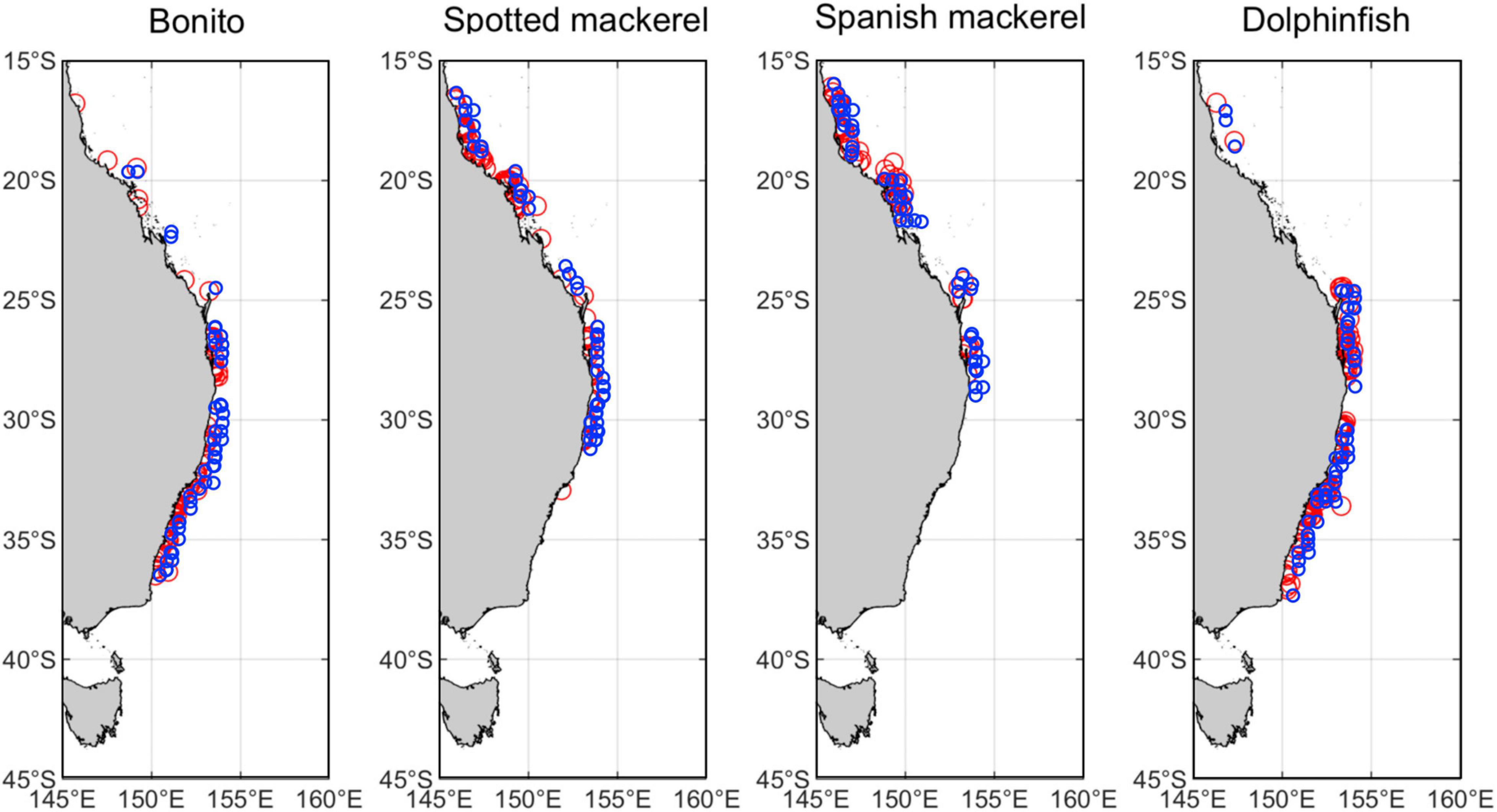
Figure 1. Map of eastern Australia displaying the spatial extent of the study region and the distribution of random samples of 300 species occurrence records (red circles) used in model fitting and 50 independent occurrences (blue circles) used in model testing for bonito (Sarda australis), spotted mackerel (Scomberomorus munroi), Spanish mackerel (Scomberomorus commerson), and dolphinfish (Coryphaena hippurus).

In order to create a binomial response variable for quantifying species’ oceanographic habitat preferences, pseudo-absence data were spatially and temporally randomised nearshore of the continental shelf-break (200-m isobath) throughout the study extent and period to characterise unsuitable habitat for each study species. A consistent dataset containing a total of 10,000 pseudo-absences was used for each species, based on Barbet-Massin et al. (2012), who recommend a large number (i.e., 10,000 or more) of randomly selected pseudo−absences for regression−type analyses for species distributions.

Oceanographic Variables

A suite of oceanographic variables known to influence the distributions of coastal-pelagic fishes (Hobday and Hartog, 2014) were downloaded from the Copernicus Marine Environment Monitoring Service¹ and matched to species occurrence and pseudo-absence data. These variables were sea surface temperature (SST; 0.05° spatial resolution), salinity (SAL; 0.25° spatial resolution), eddy kinetic energy (EKE; 0.25° spatial resolution), sea level anomaly (SLA; 0.25° spatial resolution) and chlorophyll a concentration (CHL; 0.04° spatial resolution). The native spatial and temporal resolutions of oceanographic variables were used when matching species occurrence and pseudo-absence data for developing habitat models (see Supplementary Table 1), and were bilinearly interpolated to a common 0.1° grid and aggregated to a monthly temporal resolution when making spatial predictions of habitat suitability. Collinearity among predictor variables was assessed using Spearman rank correlation coefficients and variance inflation factors (VIFs). When correlated (r > 0.5 or < −0.5) variables were identified, the predictor variable with the clearest ecological interpretation from covarying pairs was retained for model selection (Zuur et al., 2013). Sea surface temperature and salinity were negatively correlated (r = −0.71) resulting in the removal of salinity from the suite of potential oceanographic predictors prior to model fitting. Given that Spearman coefficients only describe pairwise correlations, variance inflation factors (VIFs) were used to assess the effect of collinearity among the remaining explanatory variables during model fitting. VIFs for all remaining predictors were less than 1.5, indicating that collinearity among these variables was unlikely to negatively affect model performance (Zuur et al., 2007). Full descriptions of oceanographic variables available for model selection are provided in Supplementary Table 1.

Oceanographic Habitat Modelling

Generalised additive mixed effects models (GAMMs) were used to describe oceanographic habitat suitability for all species. GAMMs used a logistic link function to relate binomially distributed response variables (i.e., species occurrence or pseudo-absence) to multiple oceanographic covariates. Year was included as a random intercept term in all models to control for intraclass correlations between data collected during the same year, which may have been temporally biased due to unmeasured variation in species catch per unit effort over the study period. Non-linear responses were modelled using penalised regression spline smoothers applied using generalized cross validation, which is recommended to optimise smooth functions and to avoid overfitting to the data (Zuur et al., 2009). However, smoothers were removed from predictor variables in favour of linear terms if their effective degrees of freedom were approximately equal to 1, indicating linearity with log-of-odds transformed binomial responses variables.

A backward model selection procedure was initially applied to identify all significant oceanographic predictors from the suite of non-correlated variables. Models were further reduced using a p-value informed backward stepwise selection procedure to produce a set of explanatory models for each species that contained nested covariate combinations of decreasing complexity (Table 1). The model in this set with the lowest Akaike information criterion (AIC) value was considered the most parsimonious model. Optimal GAMMs estimated species probability of occurrence, but given that absolute probabilities are dependent on the ratio of occurrence to absence data (Pearce and Boyce, 2006) and that pseudo-absences were randomly generated, probabilities were rescaled to an index of oceanographic habitat suitability ranging from 0 (unsuitable) to 1 (optimal).

TABLE 1

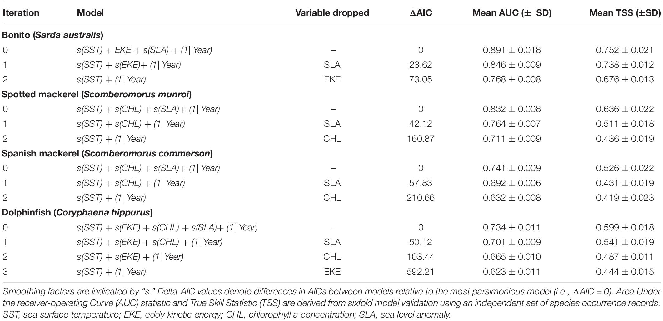
Table 1. Summary of full models for each species and nested alternatives assessed using an AIC informed model selection procedure on covariate combinations of decreasing complexity.

The accuracy and predictive skill of all models containing unique combinations of predictors were quantified using a k-fold validation approach that incorporated an independent testing dataset. To do so, the full dataset was randomly divided into six subsets (k = 6) that each contained 50 occurrence records and 2,000 pseudo-absences, and models for each species were trained on each subset of the data. Six-fold validation was used due to concerns that too few occurrence data would be available (i.e., < 50) for model fitting if the full dataset was partitioned into a greater number of folds. All models for each species were then tested against an independent set of species occurrence records (n = 50 per species; Figure 1) extracted from the Atlas of Living Australia database² and a unique set of 2000 pseudo-absences randomly sampled from the full dataset used in model fitting. These comparisons produced a set of confusion matrices for calculating two model accuracy indices, which were the mean area under the receiver operating characteristic curve (AUC) and mean true skill statistic (TSS). AUC values range from 0 to 1, where > 0.7 AUC < 0.8 indicates fair model performance, > 0.8 AUC < 0.9 indicates good performance and > 0.9 AUC indicates excellent performance (Swets, 1988; Araújo et al., 2005). Alternatively, TSS ranges from -1 to 1, where 0 denotes the threshold between models with some predictive skill (model skill increases toward 1) and models that are no better than random (model skill declines toward –1) (Allouche et al., 2006).

Range Shift Analyses

Core oceanographic habitat for each species was quantified by comparing the spatial distribution of the independent species occurrence records used in model validation with day-specific predictions of modelled habitat. Values of oceanographic habitat suitability (created with 0.1° spatial resolution) matching the spatial and temporal location of independent occurrence records (n = 50 per species) were extracted and the mean of these values was considered to represent core oceanographic habitat for each species. This approach for identifying core habitat is a data-driven alternative to selecting arbitrary threshold values (e.g., 0.5) for discriminating between species’ suitable and unsuitable environmental habitats, which commonly lack ecological basis (Liu et al., 2005; Champion et al., 2019). Defining species core habitats in this way is one option for developing comparable analyses of spatiotemporal change in species distributions, provided that (1) consistent methods are applied to quantify discrete areas of environmental habitat (e.g., core or range edge habitat), and (2) values are held constant at each time point that a spatial prediction of habitat suitability is generated.

Linear mixed effects models were used to quantify latitudinal changes in the poleward edge of core oceanographic habitats between January 1998 and December 2018. These models incorporated random terms to account for intra- and inter-annual climate variability on the latitudinal distribution of core oceanographic habitat throughout the study period. However, random effects were removed if these had low intraclass correlation coefficients (i.e., < 0.05), which indicates negligible collinearity among levels within these factors (Zuur et al., 2013). Initial range shift models fitted for all species took the form (in script notation):

$$Latitude=Year+\left(1\right|Month)+(1|ENSOstate)$$

where Latitude is the most poleward location corresponding to the distribution of each species’ core oceanographic habitat nearshore of the continental shelf-break modelled as a function of time (Year), with Month and ENSO state included as random intercept terms to account for the effects of short- and long-term climate variability on the distributions of core oceanographic habitats. ENSO state is an index of El Niño Southern Oscillation that drives oceanographic variability off eastern Australia over interannual timescales. Rates of redistribution (km per decade) of core oceanographic habitats and associated 95% confidence intervals were derived from the fixed slope parameters of linear models fitted to data extracted from monthly predictions from January 1998 to December 2018. Residual plots were assessed visually to confirm that linear mixed effects models (i.e., range shift models) satisfied the assumptions of normality and homogeneity of variance.

Data pertaining to range shift analyses are available in the Zenodo repository³. Statistical analyses were undertaken using the R programming language (R Core Team, 2017): GAMMs were fitted using the “gamm4” package (Wood and Scheipl, 2013), spatial and temporal autocorrelation was assessed using the “gstat” package (Gräler et al., 2016), k−fold cross validation was undertaken using the “dismo” package (Hijmans et al., 2013) and linear mixed effects models were fitted using the “lme4” package (Bates et al., 2015). Oceanographic habitats and data were plotted in the MATLAB computing environment (ver. 9.8, The MathWorks, Inc.).

Results

Oceanographic Habitat Models

Monthly spatial predictions of oceanographic habitat showed consistent patterns of seasonal variation among all species distributions, which underwent poleward advances during the Austral summer and autumn and equatorward retreats during winter and spring (Figure 2). Optimal models for all species contained the predictors SST and SLA, while CHL contributed to oceanographic habitat suitability for all species except bonito (Table 1). EKE was a significant predictor of the distributions of bonito and dolphinfish, but not spotted or Spanish mackerel (Supplementary Table 2). Collectively, the distributions of all study species were found to be driven by simultaneous responses to multiple oceanographic variables, with some variables (e.g., SST and CHL) contributing to the oceanographic habitat quality of multiple species.

FIGURE 2

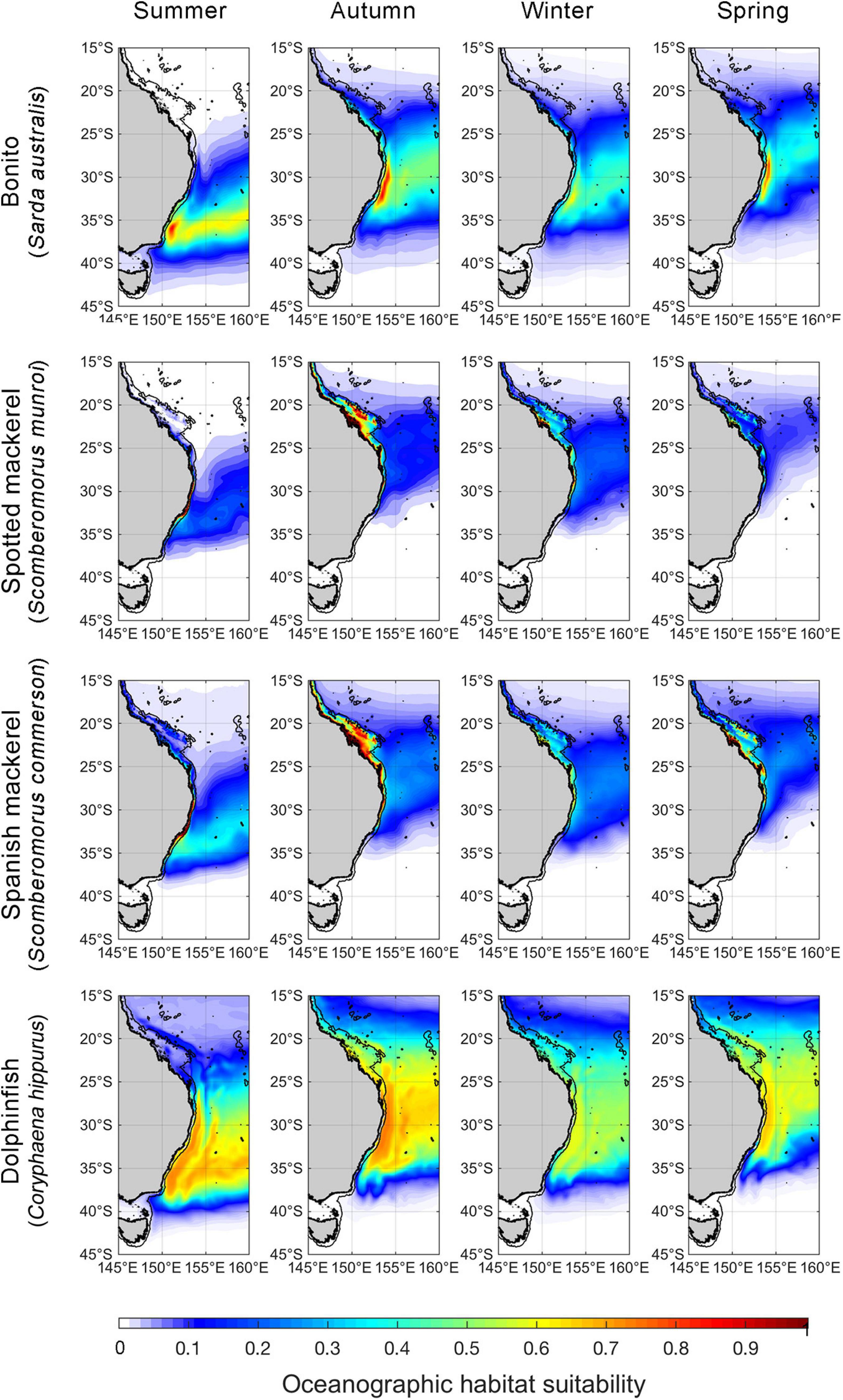
Figure 2. Spatial predictions of seasonal oceanographic habitat suitability off eastern Australia. Monthly spatial predictions were averaged for the period encompassing January 1998–December 2018 and seasonally aggregated (Summer = December to February, Autumn = March–May, Winter = June–August, Spring = September–November). The black line offshore of the coastline denotes the continental shelf-break (i.e., 200-m isobath). We note that although spatial predictions of oceanographic habitat have been extrapolated beyond the continental shelf-break to improve visual communication in this figure, range shift analyses were only undertaken on oceanographic habitat nearshore of the continental boundary.

The effects of oceanographic variables on the occurrence of all species took both non-linear and linear forms (Figure 3). SST had a consistent, unimodal effect on oceanographic habitat suitably. Peaks in optimal thermal habitat occurred between 22.5 and 24.5°C for all species. Both spotted and Spanish mackerel models produced consistent responses to SST, CHL and SLA. SLA ranging between –0.1 and 0.3 m positively affected oceanographic habitat suitability for all species, with the effect of this variable on models becoming negative toward lower and higher values than these. All covariates in each optimal oceanographic habitat model were significant at alpha level = 0.001 (Supplementary Table 2).

FIGURE 3

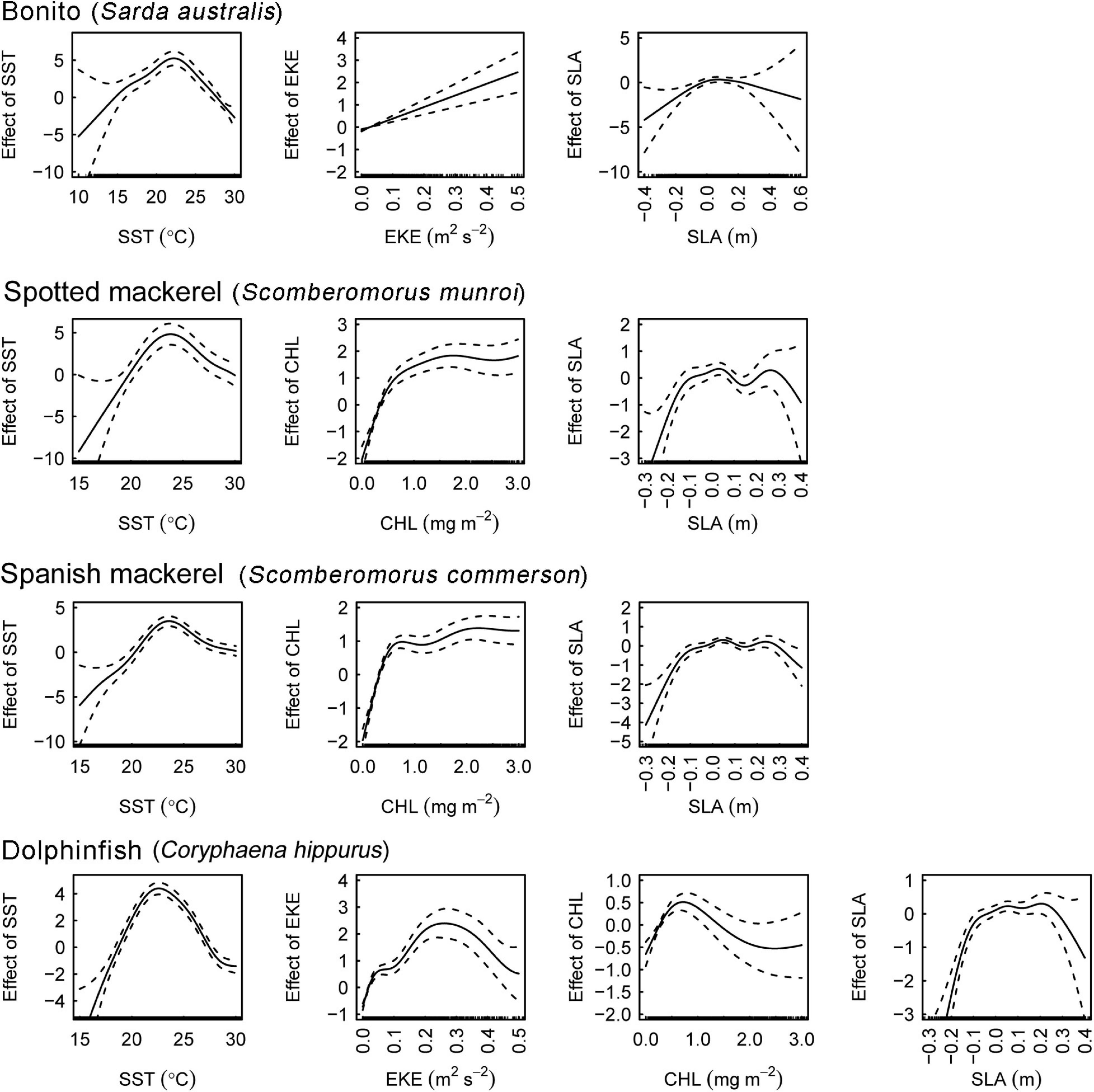
Figure 3. Partial effects of covariates on the fitted values of the optimal bonito (Sarda australis), spotted mackerel (Scomberomorus munroi), Spanish mackerel (Scomberomorus commerson), and dolphinfish (Coryphaena hippurus) habitat suitability models. Dashed lines denote 95% confidence intervals. Rugs on x−axes indicate occurrence and pseudo−absence data for each covariate. SST, sea surface temperature; EKE, eddy kinetic energy; CHL, chlorophyll a concentration; SLA, sea level anomaly.

Six−fold validation against an independent dataset not used in modelling fitting revealed that optimal models for each species had high predictive accuracy based on multiple indices of model performance (Table 1). Mean AUC and TSS values for all optimal models ranged between 0.734–0.891 and 0.526–0.752, respectively. Values within these ranges denote models with fair to good performance (Swets, 1988) and are considered reliable for conservation planning applications (Pearce and Ferrier, 2000), indicating that all optimal models produced accurate spatial predictions of species distributions for subsequent range shift analyses.

Range Shift Analyses

Habitat suitability values representative of species’ core distributions were: bonito = 0.573, spotted mackerel = 0.451, Spanish mackerel = 0.408, dolphinfish = 0.568 (Supplementary Figure 5). The poleward edge of core oceanographic habitats for all species were found to have undergone significant poleward shifts between 1998 and 2018 (Table 2 and Figure 4). Linear mixed effects models revealed that core oceanographic habitats rapidly (i.e., > 100 km per decade) moved toward higher latitudes for all species over the study period (Figure 5). However, rates of redistribution varied by approximately 130 km per decade among coastal-pelagic fishes, with core habitat shifting most rapidly for Spanish mackerel (278.6 km per decade), followed by spotted mackerel (269.7 km per decade), bonito (244.2 km per decade) and dolphinfish (148.7 km per decade; Table 2).

TABLE 2

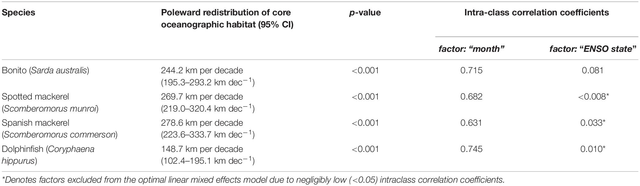
Table 2. Summary of range shift analyses.

FIGURE 4

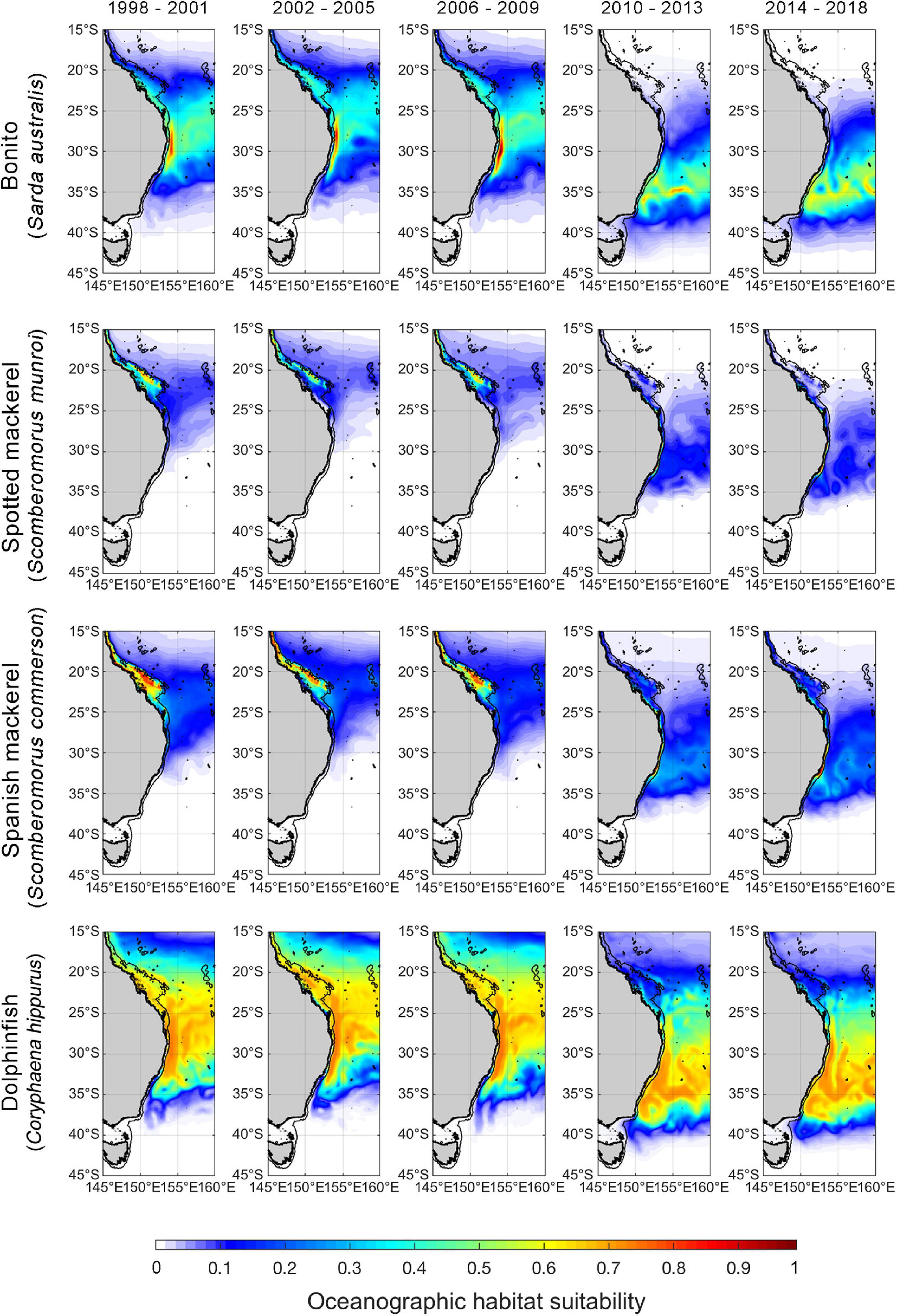
Figure 4. Spatial predictions of Autumn oceanographic habitat suitability off eastern Australia from January 1998 to December 2018. Monthly predictions have been averaged into 4-year time bins to aid visualisation of temporal trends. The black line offshore of the coastline denotes the continental shelf-break (i.e., 200-m isobath). We note that although spatial predictions of oceanographic habitat have been extrapolated beyond the continental shelf-break to improve visual communication in this figure, range shift analyses were only undertaken on oceanographic habitat nearshore of the continental shelf boundary.

FIGURE 5

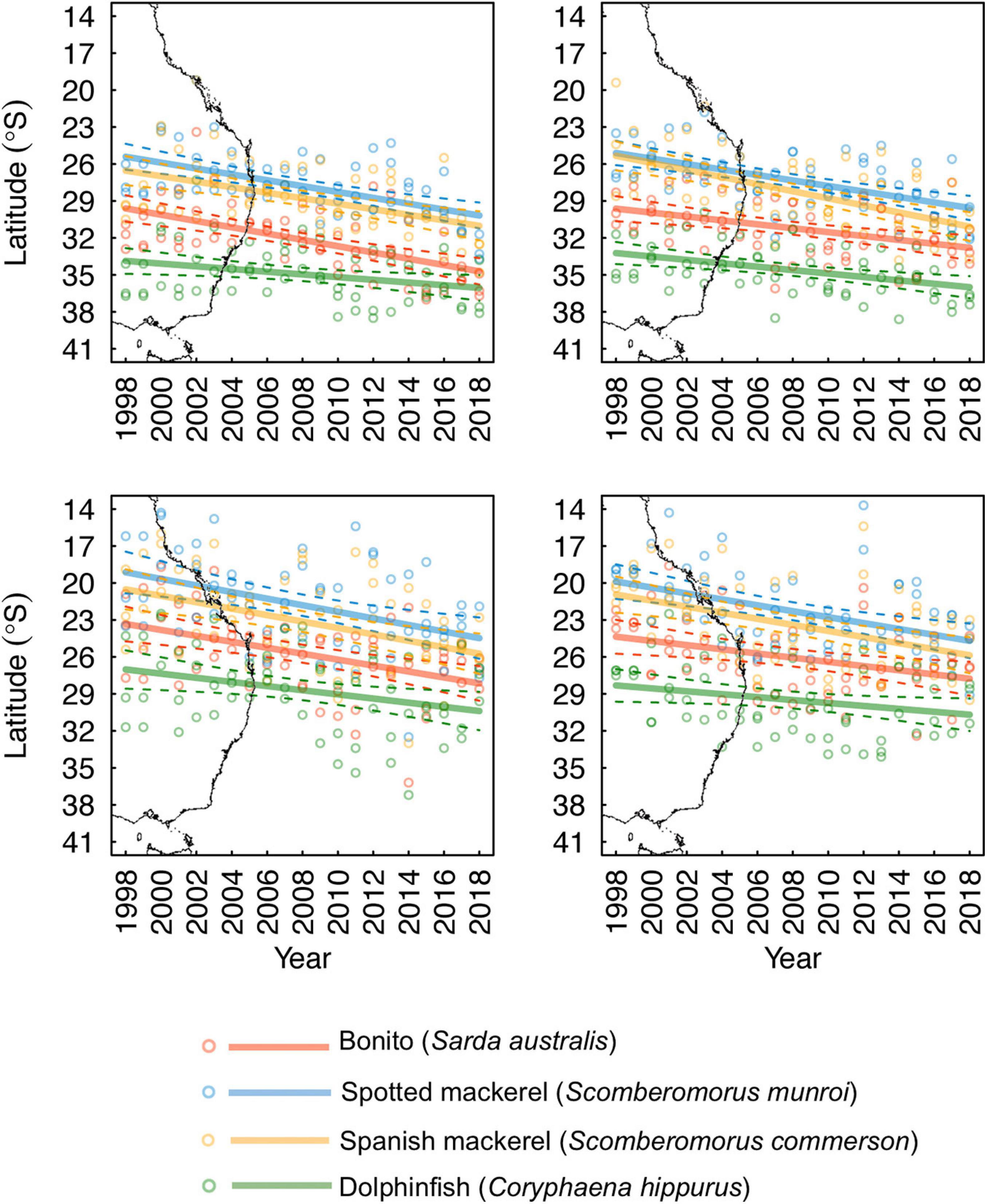
Figure 5. Seasonally explicit latitudinal trends in monthly predictions of the poleward edge of species’ core oceanographic habitats nearshore of the continental shelf-break (dashed lines denote 95% confidence intervals). The east Australian coastline has been underlaid to aid visual interpretation of the trends presented.

Poleward shifts in core oceanographic habitat occurred over a relatively lower range of latitudes for both spotted and Spanish mackerel than range shifts identified for bonito and dolphinfish (Figures 4, 5). The random “month” term was retained in all linear mixed effects models (Table 2), indicating that monthly variability in regional oceanography drove spatial variation in the distribution of core habitat for all species. However, the random “ENSO state” term was dropped from the dolphinfish and both spotted and Spanish mackerel models but retained in the bonito model (Table 2), indicating that the distribution of core habitat for bonito, but not any other species analysed, was marginally dependent on ENSO during the study period.

Discussion

By developing comparable analyses of spatial shifts in the distribution of core habitats for four coastal-pelagic fishes from a warming western boundary current, we found evidence for rapid (i.e., up to ∼280 km per decade) recent poleward redistributions. These findings are consistent with climate-driven range shifts in over 30,000 species globally that show marine taxa moving to higher latitudes six times faster than their terrestrial counterparts (Lenoir et al., 2020) and support the results of previous research demonstrating rapid climate-driven redistributions in coastal-pelagic fishes (Hill et al., 2015). However, we found that rates of redistribution varied by approximately 130 km per decade among species, highlighting that subtle differences in species’ environmental responses can manifest in highly variable rates of climate-driven range shifts.

Our analyses revealed that species’ core oceanographic habitats have shifted poleward by between ∼312 and 585 km since 1998 in response to climate−driven changes in regional oceanography. This range exceeds rates of poleward redistribution predicted for yellowtail kingfish (Seriola lalandi; approximately 240 km since 1996) and black marlin (Istiompax indica; 140 km between 1999 and 2013) off eastern Australia quantified using correlative analyses comparable to those applied here (Hill et al., 2015; Champion et al., 2018). Taken together, these findings indicate that poleward range shifts in core oceanographic habitat for coastal-pelagic fishes off eastern Australia are generally exceeding 100 km per decade, with predictions for some species (e.g., bonito and both spotted and Spanish mackerel) in excess of 200 km per decade. Given the north-south orientation of Australia’s east coast, poleward shifts of this magnitude may considerably alter the availability of resources to fisheries along the coast (e.g., Selden et al., 2020). Out-of-range observations logged by recreational anglers with the Range Extension Database and Mapping project (Redmap; Pecl et al., 2019) provide observational support for predicted shifts in coastal-pelagic fish distributions. For example, recreational catches of yellowtail kingfish off eastern Tasmania and dolphinfish off southern NSW have become increasingly reported via Redmap website and smartphone applications since the inception of this citizen science project in 2009 (Stuart-Smith et al., 2016; Fogarty et al., 2017). These catch records concur with predictions of increasing environmental suitability for these species off south-eastern Australia due to changing oceanographic conditions (Champion et al., 2018). Based on relative rates of poleward redistributions quantified using standardised methods, our results suggest that fishing opportunity off south-eastern Australia is likely to be most rapidly increasing for Spanish mackerel, followed by spotted mackerel, bonito and dolphinfish. While our analysis was developed to infer potential increases in fishing opportunity at higher latitudes, and thus quantified and compared shifts in the leading edge of oceanographic habitats, poleward shifts in the trailing edge of suitable habitat may manifest in reduced fishing opportunity at lower latitudes. For example, projected redistributions for truly pelagic fishes off eastern Australia have found that trailing edges of environmental habitat are likely to shift poleward more rapidly than leading edges in the future (Robinson et al., 2015), suggesting that losses in fishing opportunity at lower latitudes may outpace increases in opportunity at higher latitude. We acknowledge that our predictions of habitat suitability do not reflect species realised distributions directly due to their reliance on correlative relationships between species and available environmental conditions (Elith et al., 2010), which also do not incorporate the effects of biotic interactions on species distributions. Nevertheless, our findings illustrate how the redistribution of suitable oceanographic habitat for recreationally important fishes can be estimated using publicly available data to understand changes in fishing opportunity and inform fisheries adaptation.

The application of a consistent methodology and dataset for developing comparable range shift analyses was a crucial aspect of this study as methodological difference have been found to explain approximately 22% of variation in rates of climate-driven redistributions (Brown et al., 2016). For example, studies utilising continuous and consistent time series more accurately quantify rates of species redistributions than estimates based on infrequent data that may confound short-term variability with long-term trends (Brown et al., 2016; Fredston-Hermann et al., 2020). Therefore, our range shift estimates based on monthly predictions of species’ core habitats over 21 years (i.e., n = 252 per species) are likely to be more robust to short-term oceanographic variability occurring during this period than, for example, analyses based on seasonal or annual data. Although redistribution analyses using infrequent measurements commonly produce estimates of change that exceed studies using continuous time series (Brown et al., 2016), our results markedly exceed previous rates quantified for nearshore and truly pelagic fishes off eastern Australia. For example, historical analyses utilising observational data of 50 nearshore fishes identified an average rate of poleward redistribution of 38 km per decade (Sunday et al., 2015), while climate-driven redistributions for 16 pelagic fishes not analysed here averaged less than 50 km per decade (Hobday, 2010). While it is probable that rates of poleward redistributions in coastal-pelagic fishes are exceeding those of other marine fishes off eastern Australia, it is also possible that methodological differences between studies account for variation between our results and previously documented rates of redistribution. For example, our analyses incorporated species responses to multiple oceanographic variables analysed over a recent historical period, while previous research has utilised observational data (Sunday et al., 2012; Malcolm and Scott, 2016), correlative relationships with single environmental covariates (e.g., SST only; Hobday, 2010) and scenario-based projections of future ocean conditions (Robinson et al., 2015) to quantify rates of redistribution. Despite methodological difference preventing robust comparisons between our findings and previous research, results from our standardised analysis highlight that marine fishes from eastern Australia’s are likely to be undergoing poleward shifts in distribution more rapidly than previously thought.

Robust estimates of species responses to environmental conditions underpin climate change vulnerability assessments (Pacifici et al., 2015; Foden et al., 2019) and the subsequent prioritisation of species within conservation and adaptation strategies (Watson et al., 2013). Trait-based, correlative and mechanistic analyses represent the three primary approaches supporting climate change vulnerability assessments of species (Foden et al., 2019). By using species distribution or habitat suitability models to compare rates of range change for four coastal-pelagic fishes, we demonstrate the utility of correlative analyses for discriminating between the sensitivity of species distributions to climate change. Despite all species assessed being likely to receive similar climate sensitivity scores within trait-based assessments (e.g., using the methods of Pecl et al., 2014), correlative analyses identified variation in species responses. For example, the distribution of Spanish mackerel was found to be most sensitive to the environmental effects of climate change off eastern Australia, followed by the distributions of spotted mackerel, bonito and dolphinfish. These results demonstrate the utility of correlative methods for identifying species that are most likely to attract increasing fishing effort in novel poleward environments under climate change, and for prioritising the development of climate-sensitive fisheries management strategies for marine fishes that are undergoing climate-driven redistributions.

Data Availability Statement

The raw data supporting the conclusions of this article will be made available by the authors, without undue reservation.

Ethics Statement

Ethical review and approval was not required for the animal study because no animal collection was undertaken.

Author Contributions

CC conceptualised the research question and designed the study approach with input from MC. CC and SB extracted and processed oceanographic data. CC undertook the statistical and spatial analyses with assistance from SB. CC, SB, and MC wrote the manuscript. All authors contributed to the article and approved the submitted version.

Funding

This work was contributing to the NSW Primary Industries Climate Change Research Strategy, funded by the NSW Climate Change Fund.

Conflict of Interest

The authors declare that the research was conducted in the absence of any commercial or financial relationships that could be construed as a potential conflict of interest.

Acknowledgments

We are grateful to all of the citizen scientists who have contributed to the New South Wales (NSW) Department of Primary Industries Gamefish Tagging Program since its inception in 1973.

Supplementary Material

The Supplementary Material for this article can be found online at: https://www.frontiersin.org/articles/10.3389/fmars.2021.622299/full#supplementary-material

Footnotes

1. ^ https://marine.copernicus.eu
2. ^ https://www.ala.org.au
3. ^ https://doi.org/10.5281/zenodo.4475997

References

Allouche, O., Tsoar, A., and Kadmon, R. (2006). Assessing the accuracy of species distribution models: prevalence, kappa and the true skill statistic (TSS). J. Appl. Ecol. 43, 1223–1232. doi: 10.1111/j.1365-2664.2006.01214.x

CrossRef Full Text | Google Scholar

Araújo, M. B., Pearson, R. G., Thuiller, W., and Erhard, M. (2005). Validation of species–climate impact models under climate change. Glob. Chang. Biol. 11, 1504–1513. doi: 10.1111/j.1365-2486.2005.01000.x

CrossRef Full Text | Google Scholar

Barbet-Massin, M., Jiguet, F., Albert, C. H., and Thuiller, W. (2012). Selecting pseudo-absences for species distribution models: how, where and how many? Methods Ecol. Evol. 3, 327–338. doi: 10.1111/j.2041-210x.2011.00172.x

CrossRef Full Text | Google Scholar

Bates, D., Mächler, M., Bolker, B., and Walker, S. (2015). Fitting linear mixed-effects models using lme4. J. Stat. Softw. 67, 1–48.

Google Scholar

Bonebrake, T. C., Brown, C. J., Bell, J. D., Blanchard, J. L., Chauvenet, A., Champion, C., et al. (2018). Managing consequences of climate-driven species redistribution requires integration of ecology, conservation and social science. Biol. Rev. 93, 284–305. doi: 10.1111/brv.12344

PubMed Abstract | CrossRef Full Text | Google Scholar

Briscoe, D. K., Hobday, A. J., Carlisle, A., Scales, K., Eveson, J. P., Arrizabalaga, H., et al. (2016). Ecological bridges and barriers in pelagic ecosystems. Deep Sea Res. Part II Top. Stud. Oceanogr. 140, 182–192. doi: 10.1016/j.dsr2.2016.11.004

CrossRef Full Text | Google Scholar

Brodie, S., Hobday, A. J., Smith, J. A., Everett, J. D., Taylor, M. D., Gray, C. A., et al. (2015). Modelling the oceanic habitats of two pelagic species using recreational fisheries data. Fish. Oceanogr. 24, 463–477. doi: 10.1111/fog.12122

CrossRef Full Text | Google Scholar

Brodie, S. J., Thorson, J. T., Carroll, G., Hazen, E. L., Bograd, S., Haltuch, M. A., et al. (2019). Trade-offs in covariate selection for species distribution models: a methodological comparison. Ecography 43, 11–24. doi: 10.1111/ecog.04707

CrossRef Full Text | Google Scholar

Brown, C. J., O’connor, M. I., Poloczanska, E. S., Schoeman, D. S., Buckley, L. B., Burrows, M. T., et al. (2016). Ecological and methodological drivers of species’ distribution and phenology responses to climate change. Glob. Chang. Biol. 22, 1548–1560. doi: 10.1111/gcb.13184

PubMed Abstract | CrossRef Full Text | Google Scholar

Cai, W., Shi, G., Cowan, T., Bi, D., and Ribbe, J. (2005). The response of the Southern Annular Mode, the East Australian Current, and the southern mid-latitude ocean circulation to global warming. Geophys. Res. Lett. 32, 1–4.

Google Scholar

Champion, C., Hobday, A. J., Tracey, S. R., and Pecl, G. T. (2018). Rapid shifts in distribution and high-latitude persistence of oceanographic habitat revealed using citizen science data from a climate change hotspot. Glob. Chang. Biol. 24, 5440–5453. doi: 10.1111/gcb.14398

PubMed Abstract | CrossRef Full Text | Google Scholar

Champion, C., Hobday, A. J., Zhang, X., Pecl, G. T., and Tracey, S. R. (2019). Changing windows of opportunity: past and future climate-driven shifts in temporal persistence of kingfish (Seriola lalandi) oceanographic habitat within south-eastern Australian bioregions. Mar. Freshw. Res. 70, 33–42. doi: 10.1071/mf17387

CrossRef Full Text | Google Scholar

Chen, I.-C., Hill, J. K., Ohlemüller, R., Roy, D. B., and Thomas, C. D. (2011). Rapid range shifts of species associated with high levels of climate warming. Science 333, 1024–1026. doi: 10.1126/science.1206432

PubMed Abstract | CrossRef Full Text | Google Scholar

Dell, J. T., Wilcox, C., Matear, R. J., Chamberlain, M. A., and Hobday, A. J. (2015). Potential impacts of climate change on the distribution of longline catches of yellowfin tuna (Thunnus albacares) in the Tasman sea. Deep Sea Res. Part II Top. Stud. Oceanogr. 113, 235–245. doi: 10.1016/j.dsr2.2014.07.002

CrossRef Full Text | Google Scholar

Dempster, T. (2004). Biology of fish associated with moored fish aggregation devices (FADs): implications for the development of a FAD fishery in New South Wales. Australia. Fish. Res. 68, 189–201. doi: 10.1016/j.fishres.2003.12.008

CrossRef Full Text | Google Scholar

Elith, J., Kearney, M., and Phillips, S. (2010). The art of modelling range-shifting species. Methods Ecol. Evol. 1, 330–342.

Google Scholar

Feary, D. A., Pratchett, M. S., Emslie, M. J., Fowler, A. M., Figueira, W. F., Luiz, O. J., et al. (2014). Latitudinal shifts in coral reef fishes: why some species do and others do not shift. Fish Fish. 15, 593–615. doi: 10.1111/faf.12036

CrossRef Full Text | Google Scholar

Foden, W. B., Young, B. E., Akçakaya, H. R., Garcia, R. A., Hoffmann, A. A., Stein, B. A., et al. (2019). Climate change vulnerability assessment of species. Wiley Interdiscip. Rev. Clim. 10:e551.

Google Scholar

Fogarty, H. E., Burrows, M. T., Pecl, G. T., Robinson, L. M., and Poloczanska, E. S. (2017). Are fish outside their usual ranges early indicators of climate-driven range shifts? Glob. Chang. Biol. 23, 2047–2057. doi: 10.1111/gcb.13635

PubMed Abstract | CrossRef Full Text | Google Scholar

Fogarty, H. E., Cvitanovic, C., Hobday, A. J., and Pecl, G. T. (2019). Prepared for change? An assessment of the current state of knowledge to support climate adaptation for Australian fisheries. Rev. Fish Biol. Fish. 29, 877–894. doi: 10.1007/s11160-019-09579-7

CrossRef Full Text | Google Scholar

Fredston-Hermann, A., Selden, B., Pinsky, M., Gaines, S. D., and Halpern, B. S. (2020). Cold range edges of marine fishes track climate change better than warm edges. Glob. Chang. Biol. 26, 2908–2922. doi: 10.1111/gcb.15035

CrossRef Full Text | Google Scholar

Hazen, E. L., Jorgensen, S., Rykaczewski, R. R., Bograd, S. J., Foley, D. G., Jonsen, I. D., et al. (2013). Predicted habitat shifts of Pacific top predators in a changing climate. Nat. Clim. Change 3:234. doi: 10.1038/nclimate1686

CrossRef Full Text | Google Scholar

Gräler, B., Pebesma, E., and Heuvelink, G. (2016). Spatio-temporal interpolation using gstat. R J. 8, 204–218. doi: 10.32614/RJ-2016-014

CrossRef Full Text | Google Scholar

Hijmans, R. J., Phillips, S. J., Leathwick, J. R., and Elith, J. (2013). Dismo: Species Distribution Modeling. R package version 1.1-4. https://CRAN.R-project.org/package=dismo

Google Scholar

Hill, N. J., Tobin, A. J., Reside, A. E., Pepperell, J. G., and Bridge, T. C. (2015). Dynamic habitat suitability modelling reveals rapid poleward distribution shift in a mobile apex predator. Glob. Chang. Biol. 22, 1086–1096. doi: 10.1111/gcb.13129

PubMed Abstract | CrossRef Full Text | Google Scholar

Hobday, A. J. (2010). Ensemble analysis of the future distribution of large pelagic fishes off Australia. Prog. Oceanogr. 86, 291–301. doi: 10.1016/j.pocean.2010.04.023

CrossRef Full Text | Google Scholar

Hobday, A. J., and Hartog, J. R. (2014). Derived ocean features for dynamic ocean management. Oceanography 27, 134–145. doi: 10.5670/oceanog.2014.92

CrossRef Full Text | Google Scholar

Hobday, A. J., and Pecl, G. T. (2014). Identification of global marine hotspots: sentinels for change and vanguards for adaptation action. Rev. Fish Biol. Fish. 24, 415–425. doi: 10.1007/s11160-013-9326-6

CrossRef Full Text | Google Scholar

Holbrook, N. J., and Bindoff, N. L. (1997). Interannual and decadal temperature variability in the southwest Pacific Ocean between 1955 and 1988. J. Clim. 10, 1035–1049. doi: 10.1175/1520-0442(1997)010<1035:iadtvi>2.0.co;2

CrossRef Full Text | Google Scholar

Lenoir, J., Bertrand, R., Comte, L., Bourgeaud, L., Hattab, T., Murienne, J., et al. (2020). Species better track climate warming in the oceans than on land. Nat. Ecol. Evol. 4, 1044–1059. doi: 10.1038/s41559-020-1198-2

CrossRef Full Text | Google Scholar

Liu, C., Berry, P. M., Dawson, T. P., and Pearson, R. G. (2005). Selecting thresholds of occurrence in the prediction of species distributions. Ecography 28, 385–393. doi: 10.1111/j.0906-7590.2005.03957.x

CrossRef Full Text | Google Scholar

Luiz, O. J., Madin, J. S., Robertson, D. R., Rocha, L. A., Wirtz, P., and Floeter, S. R. (2012). Ecological traits influencing range expansion across large oceanic dispersal barriers: insights from tropical Atlantic reef fishes. Proc. R. Soc. B Biol. Sci. 279, 1033–1040. doi: 10.1098/rspb.2011.1525

PubMed Abstract | CrossRef Full Text | Google Scholar

Malcolm, H., and Scott, A. (2016). Range extensions in anemonefishes and host sea anemones in eastern Australia: potential constraints to tropicalisation. Mar. Freshw. Res. 68, 1224–1232. doi: 10.1071/mf15420

CrossRef Full Text | Google Scholar

Martínez, B., Radford, B., Thomsen, M. S., Connell, S. D., Carreño, F., Bradshaw, C. J. A., et al. (2018). Distribution models predict large contractions of habitat-forming seaweeds in response to ocean warming. Divers. Distrib. 24, 1350–1366. doi: 10.1111/ddi.12767

CrossRef Full Text | Google Scholar

McHenry, J., Welch, H., Lester, S. E., and Saba, V. (2019). Projecting marine species range shifts from only temperature can mask climate vulnerability. Glob. Chang. Biol. 25, 4208–4221. doi: 10.1111/gcb.14828

PubMed Abstract | CrossRef Full Text | Google Scholar

Monaco, C. J., Bradshaw, C. J., Booth, D. J., Gillanders, B. M., Schoeman, D. S., and Nagelkerken, I. (2020). Dietary generalism accelerates arrival and persistence of coral-reef fishes in their novel ranges under climate change. Glob. Chang. Biol. 26, 5564–5573. doi: 10.1111/gcb.15221

PubMed Abstract | CrossRef Full Text | Google Scholar

NSW DPI (2019). Game Fish Tagging Program. New South Wales Department of Primary Industries, Coffs Harbour. Available online at: https://www.dpi.nsw.gov.au/fishing/recreational/resources/fish-tagging/game-fish-tagging (accessed August 29, 2019).

Google Scholar

Pacifici, M., Foden, W. B., Visconti, P., Watson, J. E., Butchart, S. H., Kovacs, K. M., et al. (2015). Assessing species vulnerability to climate change. Nat. Clim. Change 5, 215–224.

Google Scholar

Pearce, J., and Ferrier, S. (2000). Evaluating the predictive performance of habitat models developed using logistic regression. Ecol. Modell. 133, 225–245. doi: 10.1016/s0304-3800(00)00322-7

CrossRef Full Text | Google Scholar

Pearce, J. L., and Boyce, M. S. (2006). Modelling distribution and abundance with presence-only data. J. Appl. Ecol. 43, 405–412. doi: 10.1111/j.1365-2664.2005.01112.x

CrossRef Full Text | Google Scholar

Pecl, G., Araujo, M., Bell, J., Blanchard, J., Bonebrake, T., Chen, I., et al. (2017). Biodiversity redistribution under climate change: impacts on ecosystems and human well-being. Science 355:eaai9214. doi: 10.1126/science.aai9214

PubMed Abstract | CrossRef Full Text | Google Scholar

Pecl, G. T., Stuart-Smith, J., Walsh, P., Bray, D., Brians, M., Burgess, M., et al. (2019). Redmap Australia: challenges and successes with a large-scale citizen science-based approach to ecological monitoring and community engagement on climate change. Front. Mar. Sci. 6:349. doi: 10.3389/fmars.2019.00349

CrossRef Full Text | Google Scholar

Pecl, G. T., Ward, T. M., Doubleday, Z. A., Clarke, S., Day, J., Dixon, C., et al. (2014). Rapid assessment of fisheries species sensitivity to climate change. Clim. Change 127, 505–520. doi: 10.1007/s10584-014-1284-z

CrossRef Full Text | Google Scholar

Pinsky, M. L., Eikeset, A. M., McCauley, D. J., Payne, J. L., and Sunday, J. M. (2019). Greater vulnerability to warming of marine versus terrestrial ectotherms. Nature 569, 108–111. doi: 10.1038/s41586-019-1132-4

PubMed Abstract | CrossRef Full Text | Google Scholar

Pinsky, M. L., Worm, B., Fogarty, M. J., Sarmiento, J. L., and Levin, S. A. (2013). Marine taxa track local climate velocities. Science 341, 1239–1242. doi: 10.1126/science.1239352

PubMed Abstract | CrossRef Full Text | Google Scholar

Poloczanska, E. S., Brown, C. J., Sydeman, W. J., Kiessling, W., Schoeman, D. S., Moore, P. J., et al. (2013). Global imprint of climate change on marine life. Nat. Clim. Change 3, 919–925.

Google Scholar

Poloczanska, E. S., Burrows, M. T., Brown, C. J., García Molinos, J., Halpern, B. S., Hoegh-Guldberg, O., et al. (2016). Responses of marine organisms to climate change across oceans. Front. Mar. Sci. 3:62.

Google Scholar

R Core Team, (2017). R: A Language and Environment for Statistical Computing. Vienna: R Foundation for Statistical Computing.

Google Scholar

Ridgway, K. (2007). Long-term trend and decadal variability of the southward penetration of the East Australian Current. Geophys. Res. Lett. 34:L13613.

Google Scholar

Robinson, L., Elith, J., Hobday, A., Pearson, R., Kendall, B., Possingham, H., et al. (2011). Pushing the limits in marine species distribution modelling: lessons from the land present challenges and opportunities. Glob. Ecol. Biogeogr. 20, 789–802. doi: 10.1111/j.1466-8238.2010.00636.x

CrossRef Full Text | Google Scholar

Robinson, L., Hobday, A., Possingham, H., and Richardson, A. J. (2015). Trailing edges projected to move faster than leading edges for large pelagic fish habitats under climate change. Deep Sea Res. Part II Top. Stud. Oceanogr. 113, 225–234. doi: 10.1016/j.dsr2.2014.04.007

CrossRef Full Text | Google Scholar

Selden, R. L., Thorson, J. T., Samhouri, J. F., Bograd, S. J., Brodie, S., Carroll, G., et al. (2020). Coupled changes in biomass and distribution drive trends in availability of fish stocks to US West Coast ports. ICES J. Mar. Sci. 77, 188–199. doi: 10.1093/icesjms/fsz211

CrossRef Full Text | Google Scholar

Sloyan, B. M., and O’Kane, T. J. (2015). Drivers of decadal variability in the Tasman Sea. J. Geophys. Res. 120, 3193–3210. doi: 10.1002/2014jc010550

CrossRef Full Text | Google Scholar

Smith, J. A., Lowry, M. B., Champion, C., and Suthers, I. M. (2016). A designed artificial reef is among the most productive marine fish habitats: new metrics to address ‘production versus attraction’. Mar. Biol. 163:188.

Google Scholar

Stuart-Smith, J., Pecl, G., Pender, A., Tracey, S., Villanueva, C., and Smith-Vaniz, W. F. (2016). Southernmost records of two Seriola species in an Australian ocean-warming hotspot. Mar. Biodiv. 48, 1579–1582. doi: 10.1007/s12526-016-0580-4

CrossRef Full Text | Google Scholar

Sunday, J. M., Bates, A. E., and Dulvy, N. K. (2012). Thermal tolerance and the global redistribution of animals. Nat. Clim. Change 2, 686–690. doi: 10.1038/nclimate1539

CrossRef Full Text | Google Scholar

Sunday, J. M., Pecl, G. T., Frusher, S., Hobday, A. J., Hill, N., Holbrook, N. J., et al. (2015). Species traits and climate velocity explain geographic range shifts in an ocean-warming hotspot. Ecol. Lett. 18, 944–953. doi: 10.1111/ele.12474

PubMed Abstract | CrossRef Full Text | Google Scholar

Swets, J. A. (1988). Measuring the accuracy of diagnostic systems. Science 240, 1285–1293. doi: 10.1126/science.3287615

PubMed Abstract | CrossRef Full Text | Google Scholar

Thorson, J. T., Rindorf, A., Gao, J., Hanselman, D. H., and Winker, H. (2016). Density-dependent changes in effective area occupied for sea-bottom-associated marine fishes. Proc. R. Soc. B Biol. Sci. 283:20161853. doi: 10.1098/rspb.2016.1853

PubMed Abstract | CrossRef Full Text | Google Scholar

Watson, J. E., Iwamura, T., and Butt, N. (2013). Mapping vulnerability and conservation adaptation strategies under climate change. Nat. Clim. Change 3, 989–994. doi: 10.1038/nclimate2007

CrossRef Full Text | Google Scholar

West, L. D., Stark, K. E., Murphy, J. J., Lyle, J. M., and Ochwada-Doyle, F. A. (2016). Survey of Recreational Fishing in New South Wales and the ACT, 2013/14. Fisheries final report series no. 149. Wollongong, NSW: NSW Department of Primary Industries.

Google Scholar

Wood, S., and Scheipl, F. (2013). gamm4: Generalized Additive Mixed Models Using mgcv and lme4. R package version 0.2-2. Available online at: http://CRAN.R-project.org/package=gamm4

Google Scholar

Zuur, A. F., Hilbe, J. M., and Ieno, E. N. (2013). A Beginner’s Guide to GLM and GLMM with R. Newburgh, NY: Highland Statistics.

Google Scholar

Zuur, A. F., Ieno, E. N., and Smith, G. M. (2007). Analysing Ecological Data. New York, NY: Springer.

Google Scholar

Zuur, A. F., Ieno, E. N., Walker, N. J., Saveliev, A. A., and Smith, G. M. (2009). Mixed Effects Models and Extensions in Ecology with R. New York, NY: Springer.

Google Scholar