Bottom–Up Impacts of Forecasted Climate Change on the Eastern Bering Sea Food Web

Introduction

Climate change is rapidly affecting marine species and ocean ecosystems worldwide (Hoegh-Guldberg and Bruno, 2010; Poloczanska et al., 2013) by warming water temperatures, increasing stratification, reducing dissolved oxygen, and altering nutrient supplies and thereby primary production (Bopp et al., 2013; Boyce and Worm, 2015; Cheng et al., 2019). This in turn limits production at higher trophic levels (Ryther, 1969; Iverson, 1990), including production that supports fisheries (Pauly and Christensen, 1995; Chassot et al., 2010; Stock et al., 2017). Climate change directly affects organisms at the individual level through impacts on physiological processes and behavioral responses, altering rates of somatic growth, mortality, and reproduction (Portner and Peck, 2010). These individual impacts are transmitted to higher levels of community organization through altered population growth rates, species distribution, community composition, and predator-prey interactions (Cheung et al., 2009; Rijnsdorp et al., 2009; Doney et al., 2012; Pinsky et al., 2013). The accumulation of these impacts affects the structure, function, and productivity across all levels of a food web (Kortsch et al., 2015; Sydeman et al., 2015).

Marine ecosystems are also simultaneously subject to the stress of fisheries, which reduces the abundance of target and non-target species, further altering community composition and species interactions (Tegner and Dayton, 1999; Steele and Schumacher, 2000; Jackson et al., 2001; Worm et al., 2009). Fishing can also lead to demographic changes in fish populations that increase their variability, making them more sensitive to changing climate conditions (Berkeley et al., 2004; Hsieh et al., 2006; Anderson et al., 2008; Hidalgo et al., 2011; Shelton and Mangel, 2011). The impacts of climate change on marine species and ocean ecosystems have ramifications for dependent communities that rely on the ocean for nutrition and income, and for the commercial fishing industry (Sumaila et al., 2011; Allison and Bassett, 2015).

The impacts of climate change on the ecosystem and the food web are becoming increasingly visible in the eastern Bering Sea. Historically, the eastern Bering Sea continental shelf has been covered by sea ice during winter and early spring, which leaves a remnant “cold pool” of bottom water (<2°C) over portions of the central shelf throughout the summer (Coachman, 1986; Wyllie-Echeverria and Wooster, 1998; Sullivan et al., 2014). The presence of the cold pool is a key biophysical feature that limits species distributions and influences community composition (Mueter and Litzow, 2008; Stevenson and Lauth, 2012, 2019; Eisner et al., 2018). Seasonal variation in the presence of sea ice and the cold pool has important implications for the timing, magnitude, and community composition of primary and secondary production (Coyle et al., 2011; Stabeno et al., 2012; Coyle and Gibson, 2017), for the recruitment of commercially important fishes (Hunt et al., 2011; Duffy-Anderson et al., 2016; Farley et al., 2016; Cooper et al., 2020), and marine mammal and seabird habitats (Cooper et al., 2013; Citta et al., 2018). Recent years (2014–2019) have seen a decline in the duration and coverage of seasonal sea-ice, a decrease in the size of the cold pool, and warming water temperatures (Stabeno and Bell, 2019; Baker et al., 2020; Danielson et al., 2020). These physical changes altered the phenology, magnitude, and species composition of the phytoplankton bloom and zooplankton community, changes which were transmitted up the food web to forage fishes, including the juvenile stages of commercial species, and to other higher trophic level predators (Sigler et al., 2016; Duffy-Anderson et al., 2019; Lomas et al., 2020). The recent reductions in sea ice coverage and warming water temperatures are in contrast with the historical record and may portend an impending shift in ecosystem structure and function (Grebmeier et al., 2006; Huntington et al., 2020).

Environmental changes associated with warming may have profound social and economic consequences. The living marine resources of the eastern Bering Sea are an important source of nutrition for coastal communities and have significant social and cultural value (Renner and Huntington, 2014; Gadamus and Raymond-Yakoubian, 2015). Additionally, the eastern Bering Sea has several valuable groundfish and crab fisheries (Fissel et al., 2017), including the fishery for walleye pollock (Gadus chalcogrammus) which has averaged ∼1.2 million tons in catch per year since the 1970s (Ianelli et al., 2017) and is the world’s second largest single-species fishery (FAO, 2019). The North Pacific Fishery Management Council (NPFMC) manages federal fisheries in Alaska for valuable fish and shellfish through the application of a polycentric decision making system founded on an ecosystem approach to management of groundfish resources that is informed by a Fisheries Ecosystem Plan (NPFMC, 2019). Two elements of the ecosystem approach to fishery management used by the NPFMC are particularly relevant to this paper: a 2 million metric ton (MMT) overall cap on annual groundfish removals; and the use of a precautionary harvest control rule that includes a buffer between the target and limit fishing mortality rates. In addition, for most species targeted in the fishery, a sloping control rule is applied where-in fishing mortality is reduced when the spawning stock biomass drops below the target biomass level, which is higher than the biomass that can produce the maximum sustainable yield (B_msy or its proxy) (NPFMC, 2018).

The NPFMC’s Fishery Ecosystem Plan informs management by projecting future stock status and ecosystem conditions that consider the interacting effects of climate change and fisheries on target and non-target species, food webs, and tradeoffs in different ocean uses to make informed decisions on sustainable resource exploitation (Spencer et al., 2019; Hollowed et al., 2020; Holsman et al., 2020; Reum et al., 2020). The Alaska Climate Integrated Modeling Project (ACLIM) was initiated by NOAA’S Alaska Fisheries Science Center to investigate these types of questions for the eastern Bering Sea (Hollowed et al., 2020). ACLIM is an integrated modeling program that links outputs from a selection of global earth system models run under Intergovernmental Panel on Climate Change (IPCC) climate scenarios to a suite of biological models to investigate the potential impacts of forecasted climate change on fish, fisheries, and the ecosystem of the eastern Bering Sea (Hollowed et al., 2020). The multi-model approach of ACLIM allows for joint consideration of the strengths and weaknesses of different model structures and facilitates the examination of different sources of uncertainty in projection results.

We developed an Ecopath with Ecosim model (EwE¹, Christensen and Pauly, 1992; Christensen and Walters, 2004) of the eastern Bering Sea to investigate the potential impacts of forecasted climate change on species and the food web, and the interactive effects of different fisheries management scenarios and climate change on modeled outcomes. The ACLIM modeling framework incorporates a coupled regional ocean and biogeochemical model to project future ocean conditions and lower trophic level dynamics (Hollowed et al., 2020). Forecasted climate change is expected to impact water temperatures, sea ice, phytoplankton, and lower trophic levels in the eastern Bering Sea (Wang et al., 2012; Hermann et al., 2019), and will have a bottom–up impact on the broader food web. There are many variables that could potentially be affected by climate change. Due to the anticipated changes at the base of the food web, we incorporate climate change impacts into food web simulations by representing the biomass of primary and secondary producer groups with projections from the climate-enhanced lower trophic level modeling. This approach specifically examines the bottom–up effects of changing biomass at lower trophic levels due to climate change, and how these changes may be transmitted up the food web to consumer groups via their trophic linkages.

Here we use our climate-enhanced dynamic food web model to ask how the impacts of forecasted climate change on lower trophic levels may affect species and the broader food web in the eastern Bering Sea, and how might those responses change under alternative climate change and fishery management scenarios? We incorporate a fisheries sub-model into our simulations that provides dynamic projections of annual catch quotas for US federally managed groundfish in the eastern Bering Sea in response to the changing status of managed stocks and in accordance with the existing fisheries management paradigm. Our primary objective was to project the biomass and catch of commercially important species and the biomass of trophic guilds to examine a range of possible outcomes at the end of the century for individual species and the food web under forecasted climate change and the prescribed fishing scenarios. Biomass trajectories of marine mammals and seabirds are also projected, many of which are protected species or whose well-being is thought to be an indicator of food web status (Sydeman et al., 2017).

Materials and Methods

Modeling Approach

Our modeling approach was to use the outputs from multiple earth system models, each run under a selection of climate change scenarios, to drive a regional ocean and biogeochemical model (Figure 1). The projected conditions from the oceanographic lower trophic level model are then used as inputs to represent climate change in the food web model. The food web model was linked to a fisheries sub-model that incorporates social and economic tradeoffs into dynamic predictions of catch quotas under different fisheries management scenarios based on the existing fisheries management paradigm. We cover each of these components of the modeling framework below.

FIGURE 1

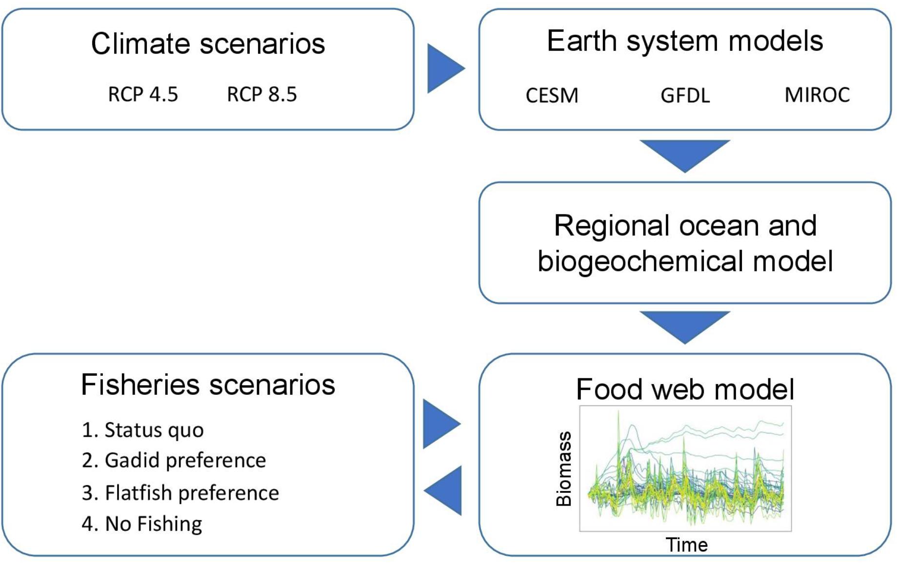
Figure 1. Overview of the ACLIM modeling framework as implemented with our food web model. The outputs from three earth system models, each driven by two IPCC AR5 climate scenarios (RCP 4.5 and 8.5), are dynamically downscaled and used to drive a regional ocean and biogeochemical model through the end of the century. The outputs from the lower trophic level modeling are used to simulate the biomass dynamics of phytoplankton and zooplankton groups in the food web model. The food web model is coupled to a fisheries sub-model that dynamically predicts annual commercial fisheries catch in response to the simulated stock status and under four different quota allocation scenarios.

Simulating Climate Change

The earth system models we use are selected from the Climate Model Intercomparison Project phase 5 (CMIP5; Taylor et al., 2012) and include, the Geophysical Fluid Dynamics Laboratory Earth System Model 2M (GFDL-ESM2M, Dunne et al., 2012), the National Center for Atmospheric Research (NCAR) Community Earth System Model (CESM, Kay et al., 2015), and the Model for Interdisciplinary Research on Climate (MIROC-ESM, Watanabe et al., 2011). These models were selected because they represent the breadth of simulation outcomes present in the suite of models included in CMIP5, and for their performance within the Bering Sea study region (Hermann et al., 2019). The earth system models were driven with two representative concentration pathways (Moss et al., 2010) from the IPCC Fifth Assessment Report (AR5). These pathways describe different trajectories for future greenhouse gas emissions, mitigation, and subsequent climate change. Two global emission scenarios were considered: RCP 8.5, which represents an unmitigated pathway with high greenhouse gas emissions; and RCP 4.5, which represents an intermediate level of mitigation and greenhouse gas emissions.

We simulate production dynamics of lower trophic level functional groups using a regional ocean circulation model based on a Regional Ocean Modeling System (ROMS) domain coupled to a lower trophic level biological model developed during the Bering Sea Ecosystem Study (BEST) Program (Gibson and Spitz, 2011) and later improved in various versions (Hermann et al., 2016; Kearney et al., 2020). The coupled biophysical model covers the Bering Sea with 10-km horizontal resolution (Bering 10K ROMS/BEST-NPZ, Hermann et al., 2016; hereafter referred to as “Bering 10K”). Bering10k is driven at the sea surface and ocean lateral boundaries by variables from the coarse resolution global earth system models mentioned above, and integrated continuously in time from 2006 to 2100; in this way, the biophysical state of the Bering Sea from the various earth system model forecast scenarios is dynamically downscaled. More details of the Bering10K and its use as a tool for dynamic downscaling can be found in Hermann et al. (2019). Because our food web model is not spatially discrete, monthly averages over our study area were extracted from the BESTNPZ output (Holsman et al., 2020) to represent biomass dynamics for small and large phytoplankton, pelagic and benthic microbes, copepods, and euphausiids in our food web model (see Supplementary Material).

Outputs from the reanalysis-forced BESTNPZ hindcast (Hermann et al., 2013, 2016) were used to force the trophic dynamics model from 1991 to 2017. Outputs from the CMIP5-forced BESTNPZ forecasts were used to simulate future climate scenarios over the period 2006 to 2099. The BESTNPZ outputs used for projections (2018–2099) were bias-corrected using differences in monthly mean and variability between the hindcast and projections during the overlapping period (2006–2017; Ho et al., 2012; Hawkins et al., 2013; see Supplementary Material and Supplementary Figure 1). The downscaled runs with the CESM model under RCP 4.5 did not go beyond 2080, so we limit our analysis of the RCP 4.5 simulations to 2080 and earlier, and any comparisons between RCP 4.5 and RCP 8.5 are also limited to 2080.

Food Web Model

We use Ecopath with Ecosim (EwE) to model the food web of the eastern Bering Sea. EwE is a biomass compartment model that integrates information on species biomass, production, consumption, diet composition, and mortality to describe the network of connections and material flows between groups in a food web (Polovina, 1984; Christensen and Walters, 2004). The equations and algorithms underlying the EwE framework are thoroughly documented elsewhere (e.g., Walters et al., 1997; Christensen and Walters, 2004). For our analysis we use Rpath² (Lucey et al., 2020, 2021), an independent version of EwE that uses the same equations and algorithms of EwE but is developed for use with the open source statistical program R (R Core Team, 2015). Using Rpath also allows us to use a region-specific fisheries sub-model that dynamically predicts fisheries catch based on harvest control rules and model-simulated stock biomass, that has also been developed for use with R (more in Fisheries Scenarios below, Faig and Haynie, 2019).

We use a previously published EwE model of the eastern Bering Sea that was calibrated to the early 1990s (1990–1994) and constructed on a scale that reflects existing fishery management regions and coincides with known distributions of several commercial groundfish stocks (Aydin et al., 2007). The region of study includes the continental shelf and upper continental slope waters between 25 and 1000 m depth, encompassing an area of ∼495,000 km² (Figure 2). The model was informed by decades of data collected in the eastern Bering Sea to support fisheries management and for monitoring protected species, trophic interactions, and lower trophic levels [see Aydin et al. (2007) for complete documentation of all model parameters and data sources].

FIGURE 2

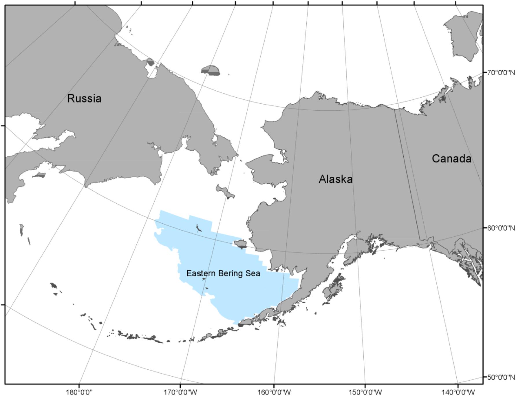
Figure 2. The area in the eastern Bering Sea described by the EwE model of Aydin et al. (2007).

The model as originally constructed was highly detailed with 129 biological groups, including 14 single-species groups with separate adult and juvenile compartments (a.k.a., stanzas). While we sought to maintain this level of detail for some commercial fish and protected species, we aggregated several species into functional groups with other species of similar life history traits, food habits, and environmental requirements in the interest of keeping the model results tractable (Supplementary Table 1). Functional groups that were aggregated together had their respective biomasses and fisheries catch summed together. The P/B, Q/B, and diet composition of the aggregated groups were averages weighted by the biomass of the original groups. We reduced the original full model to 72 biological groups, including five single-species groups with corresponding juvenile groups, two primary production groups, and three detrital compartments (pelagic, benthic, and fisheries offal) (Supplementary Table 2). Aggregating the model did not bring it out-of-balance and no modifications were necessary. This eastern Bering Sea model was originally tuned to the reference state of the early 1990s (Aydin et al., 2007), therefore we initiate our simulations in 1991.

Detritus pools are basal resources supporting the production of lower trophic levels in a food web (Rooney et al., 2006). While the biomass of detritus pools are generally unknown, we tracked the biomass of detritus as it is a key dietary component for lower trophic levels. Detritus in our food web model comes from unassimilated food, fishery offal, and mortality from sources other than predation and fisheries. Rpath calculates the biomass of detritus (if not provided by user) as the sum of inputs to detritus divided by the turnover rate of detritus (Lucey et al., 2020). We did not specify a turnover rate for detritus and used the Rpath default of 0.5. This made the detritus biomass equal to twice the detritus input.

Fisheries Catch Scenarios

During the hindcast period (1991–2017) the model was projected with the actual catch time series for groundfish and crab species (Cahalan et al., 2014) when such data were available, and the exploitation rate from the Ecopath model for components with no historical catch data. Groundfish catch during the projection period (2018–2099) was predicted using a fisheries sub-model, which predicted the catch of federally managed groundfish in the eastern Bering Sea based on estimates of acceptable biological catch (ABC). The input ABCs were used to predict the total allowable catch (TAC) and the TACs are then used to predict catch. The fisheries sub-model, known as the “ABC to TAC And Commercial Harvest model,” or ATTACH, and its documentation can be downloaded from www.github.com/amandafaig/catchfunction. The catches predicted by ATTACH are based on historical relationships between the ABCs and observed catch, modeling the historical practices of the regional fishery management council for quota setting and redistributing quota between fisheries sectors and management areas under the 2 MMT ecosystem harvest cap and the observed abilities of the fisheries to catch the allocated quotas. The ATTACH has previously been used with a multi-species size-spectrum model of the eastern Bering Sea food web (Reum et al., 2020) and a multi-species statistical catch-at-age model of walleye pollock, Pacific cod (Gadus macrocephalus), and arrowtooth flounder (Atheresthes stomias) (Holsman et al., 2020). Detailed descriptions of the equations and assumptions in ATTACH can be found in the source documentation (Faig and Haynie, 2019) and in the appendices of Holsman et al. (2020) and Reum et al. (2020).

At the end of each year during the projection period (2018–2099), we calculated ABCs for each of the federally managed groundfish stocks and commercial crab stocks using a sloped harvest control rule that mimics that used for actual management (NPFMC, 2017). We used the Ecopath-based biomass (B) and exploitation rate (F) as target values in our harvest control rule (B_target and F_target). Federally managed gadids and flatfish generally account for about 75% of the ecosystem harvest cap, and are the species of core interest in this study. The biomass and catch of gadids and flatfish in 1991 were near long-term averages, making 1991 a suitable reference year for these biological reference points. The ABCs are based on stock status during the simulation, which is evaluated as the ratio of simulated stock biomass of species i (B_i) to their target biomass (B_i,target):

$\begin{array}{c}\hfill AB{C}_i=\{\begin{array}{c}\hfill B_i*F_{i,target}\hfill \\ \hfill B_i*F_{i,target}*\frac{\left(\frac{B_i}{B_{i,target}}-\mathrm{\alpha }\right)}{\left(1.0-\mathrm{\alpha }\right)}\hfill \\ \hfill 0\hfill \end{array}\begin{array}{c}\hfill ,if\frac{B_i}{B_{i,target}}\ge 1\hfill \\ \hfill ,if\mathrm{\hspace{0.33em}0.2}<\frac{B_i}{B_{i,target}}<1\hfill \\ \hfill ,if\frac{B_i}{B_{i,target}}\le 0.2\hfill \end{array}\hfill \end{array}(1)$

α has a default value of 0.05 and is the intercept to the sloped harvest control rule where F, and thus ABC, would be equal to zero (Figure 3). We use a modified harvest control rule that sets the ABC equal to zero when the simulated stock status drops below a minimum threshold (B_i/B_i,target ≤ 0.2). This modified harvest control rule is used in Alaska for pollock and other groundfish to help maintain prey resources for protected species (NPFMC, 2018).

FIGURE 3

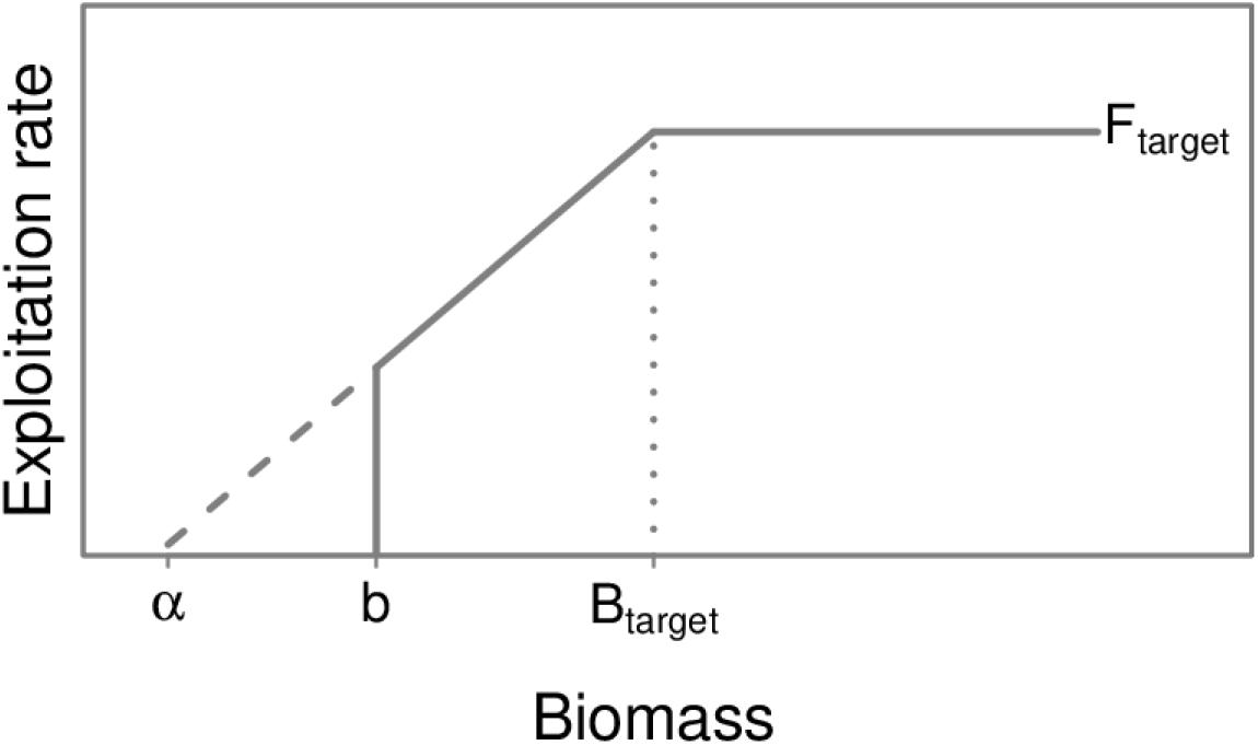
Figure 3. Schematic of the harvest control rule used to determine the acceptable biological catch of groundfish subject to the ecosystem harvest cap. The target biomass (B_target) and target exploitation rate (F_target) are the Ecopath-based biomass and exploitation rate. α is the intercept to the sloped harvest control rule where fishing mortality, and thus ABC, would be equal to zero. We use a modified harvest control rule that sets fishing mortality equal to zero when the simulated stock biomass drops below a minimum threshold of 0.2 B_target (b).

At the end of each year during the projection period (2018–2099), the simulation was paused so we could calculate ABCs for all the groundfish species (or multi-species complex) managed under the ecosystem harvest cap (Table 1). The calculated ABC values were input to the fisheries sub-model, which returned the predicted catch for those stocks in the next year of the simulation. The predicted catches were then applied to the next year of the simulation, and the simulation resumed for one more year.

TABLE 1

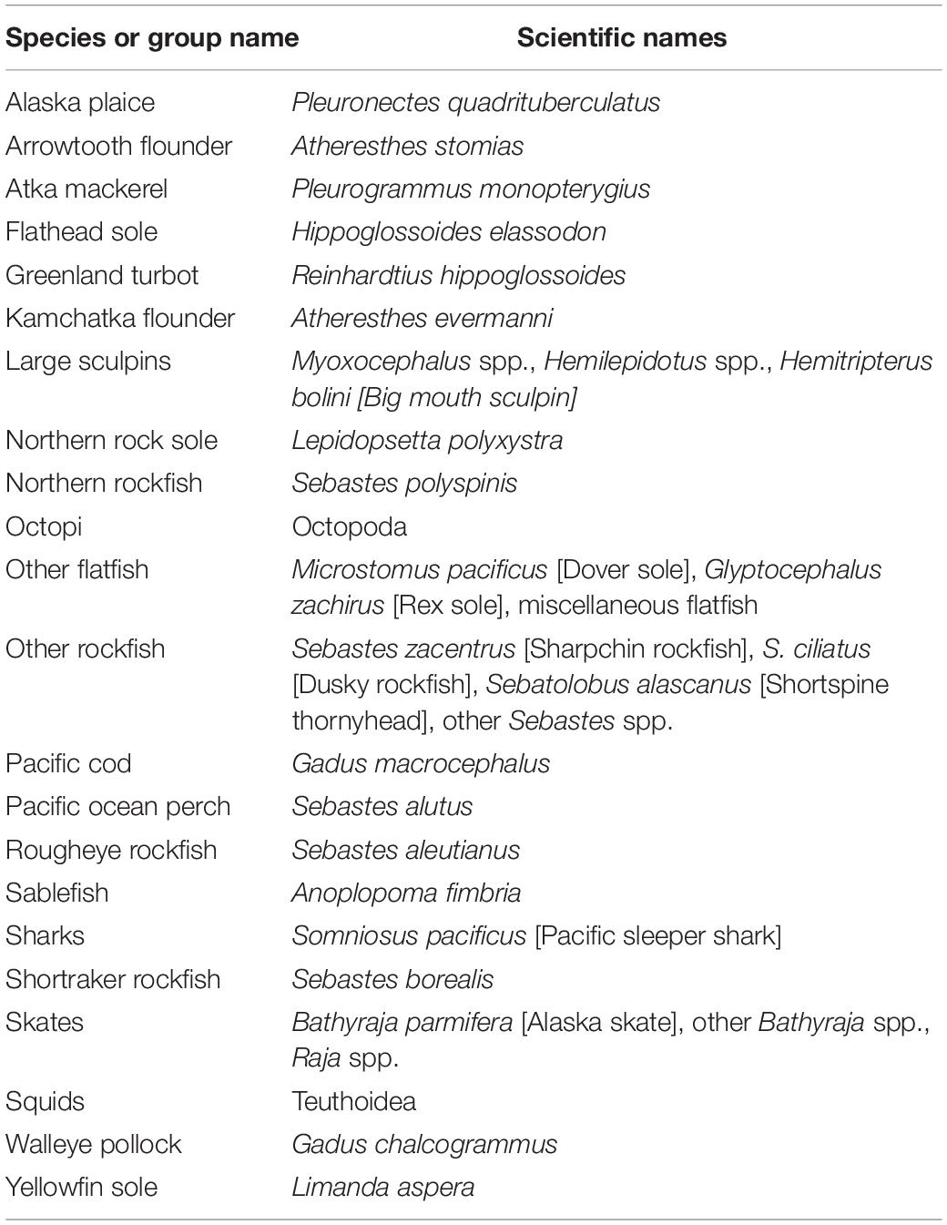
Table 1. Groundfish species or species complexes managed under the Bering Sea/Aleutian Islands ecosystem harvest cap.

Given the constraint of the two million ton ecosystem harvest cap there are several ways that quota could be allocated in the future. The fisheries sub-model predicts catch under four quota allocation scenarios that are subject to the ecosystem cap and have been vetted through the NPFMC (Hollowed et al., 2020): (1) a status quo scenario that reflects the current practices and decisions of the fishery management council, and assumes no significant changes to those practices are made; (2) a gadid preference scenario with an expansion of pollock and Pacific cod quota (up to 10% increase) under the cap and at the expense of other groundfish fisheries; (3) a flatfish preference scenario that included an increase in the combined flatfish quota (up to 30%) under the cap and at the expense of pollock and Pacific cod; and (4) a scenario where no fishing is allowed. The no fishing scenario is intended to highlight how species and the food web may fare in the absence of fishing but still subject to simulated climate change.

The individual quotas set by the regional fishery management council, are less than the ABCs determined in the respective stock assessments. The sum of the groundfish quotas must fit under the ecosystem cap, so some stocks are fished well below their respective ABC (Witherell et al., 2000). For example, the quotas for flatfish have historically been set below their respective ABCs to allow for larger harvests of pollock and Pacific cod under the ecosystem cap (Witherell, 1995). The fisheries sub-model reflects these historical practices when making catch projections. For example, the catch of arrowtooth flounder and northern rock sole are both limited to a constant maximum catch as long as their stock status stays above the threshold biomass (B_i/B_i,target ≥ 1). However, under the flatfish preference scenario, the constant maximum catch on northern rock sole can be relaxed when their biomass is greater than B_target and the combined ABC of pollock and Pacific cod is above ∼1.4 million tons. Above that level, 10% of the predicted gadid catch is reallocated to flatfish and can increase the catch of northern rock sole above their constant catch maximum.

Analysis of Results

We focus our analysis on a core group of six species that are currently of economic and ecological importance in the study region: walleye pollock, Pacific cod, yellowfin sole (Limanda aspera), northern rock sole (Lepidopsetta polyxystra), arrowtooth flounder, and snow crab (Chionoecetes opilio). We track the biomass trajectories and catch projections for these core species through the end of the century. Additionally, we track the biomass of marine mammals and seabirds, whose condition may be an indicator of food web status and prey availability. The biomass projections for all functional groups included in the food web model, and under all scenarios, can be found in the Supplementary Material. As an indicator of ecosystem status and food web structure, we also track the biomass of trophic guilds including, apex predators, benthic foragers, motile epifauna, pelagic foragers, structural epifauna, shrimp and other zooplankton, and infauna (Table 2).

TABLE 2

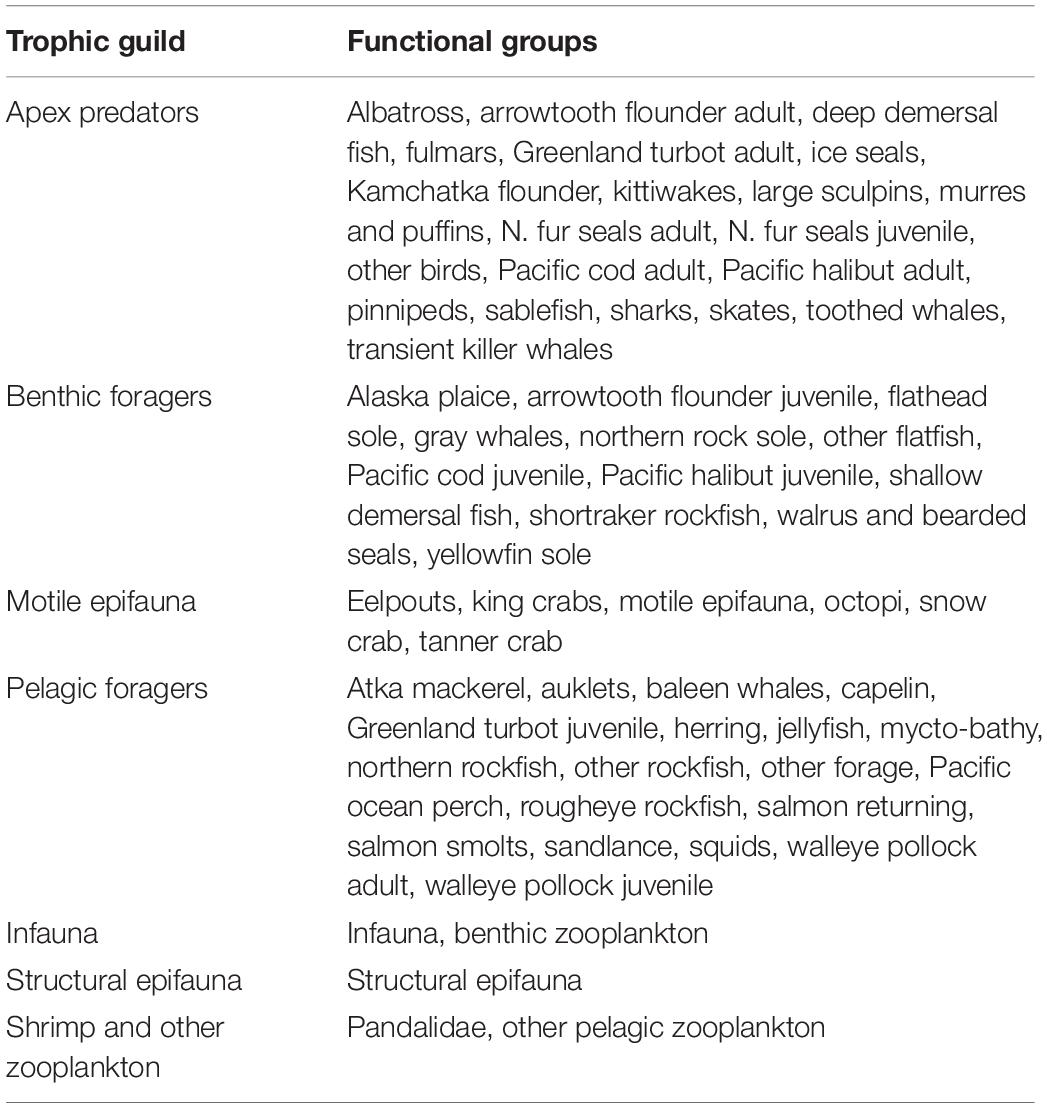
Table 2. The composition of trophic guilds.

Within trophic guilds, we examined the change in biomass between the end of the hindcast period (2008–2017) and the last 10 years of the projection period (2071–2080) run under both RCPs. Within each trophic guild, we separated results by earth system model, RCP, and by fishing scenario. Within each earth system model-RCP-fishing scenario combination, we looked at the distribution of the percent change in biomass for functional groups within each trophic guild. This distribution of outcomes does not consider any process error arising from inherent variability in the population dynamics, parameter uncertainty in our food web model, uncertainty in the implementation of our quota allocation scenarios, or any error in our observation of stock status. We calculated the change in biomass as the difference between the mean biomass over the last 10 years of the hindcast period (2008–2017) and the last 10 years of the projection period (2071–2080), divided by the mean biomass over the last 10 years of the hindcast period. The apex predator guild includes 21 functional groups, benthic foragers includes 12, motile epifauna 6, and pelagic foragers 19. We did not include infauna, structural epifauna, and shrimp and other zooplankton in this analysis as those guilds consist of only one or two functional groups and we therefore could not describe a range of outcomes.

Sensitivity Analysis

A mass-balanced food web model represents only one of many possible mass-balanced food web configurations. Additionally, there are varying degrees of uncertainty about all the model parameters, with some parameters being well supported by data and others not. Simulations with alternative model parameterizations could lead to divergent outcomes for species and the food web. We evaluated the sensitivity of our projections to parameter uncertainty using a Monte Carlo routine to generate an ensemble of alternative Ecosim parameter sets from our Ecopath model, following the approach of Whitehouse and Aydin (2020). We conducted identical simulations with each ensemble member to examine how sensitive our simulation results were to uncertainty in parameter estimates (biomass, P/B, Q/B, diet composition, and other mortality [M₀]), and the predator-prey functional response (i.e., vulnerability). We used a data pedigree to describe the quality of the original parameter estimates. Each pedigree score corresponds to a prescribed range as a proportion of the original parameter estimate (coefficient of variation, CV). Entire sets of Ecosim parameters were drawn from distributions centered on the balanced model estimates and bounded by their respective CVs. Vulnerability ranges from one to infinity for each predator/prey link, and is centered on 2.0; the value represents the ratio of top–down to bottom–up control plus 1.0 (so the center of 2.0 represents a balance of top–down versus bottom–up control). However, values beyond 91 are difficult to distinguish from infinity (Gaichas et al., 2012), therefore, we allowed vulnerability to vary from 1.01 to 91 using a log-uniform distribution for all trophic links. The generated Ecosim parameter sets were subjected to a 100-year burn-in to eliminate unstable configurations (e.g., ecosystems with functional groups whose biomass decreases to zero, or biomass grows without limit). Each of the retained ecosystems was subjected to a simulation with climate-forcing under the GFDL-RCP 8.5 emission scenario and the status quo scenario of the fisheries sub-model. For each retained ecosystem, we calculated the percent change in biomass for each functional group as the change in the mean biomass from the final 10 years of the simulation (2090–2099) relative to the mean of the respective group’s biomass from the final 10 years of the hindcast period (2008–2017). A more detailed description of the sensitivity analysis can be found in the Supplementary Material and in Whitehouse and Aydin (2020).

Results

Lower Trophic Level Projections

Our food web model projected declining trends in annual mean biomass for most lower trophic level functional groups (Figure 4). Across the three downscaled projections, Hermann et al. (2019) predicted a net decrease for the combined biomass of small and large phytoplankton. These two primary producer groups were modeled as separate functional groups in our food web model. In our study area, small phytoplankton biomass was projected to decrease by the end of the century across all three earth system model projections and both RCPs. However, large phytoplankton was projected to have a modest biomass increase in the GFDL and CESM projections and a more substantial increase in biomass was predicted under the MIROC projection (Supplementary Figure 2). Euphausiids gradually decrease through the rest of the century to values near the minimum over the hindcast. Copepod biomass also declined, and by mid-century was well below minimum values observed during the hindcast. Pelagic and benthic microbes did not show a clear trend and finished the century within the range of values from the hindcast. Both pelagic and benthic detritus pools decreased toward the end of the century and stabilized at values below their mean values during the hindcast period.

FIGURE 4

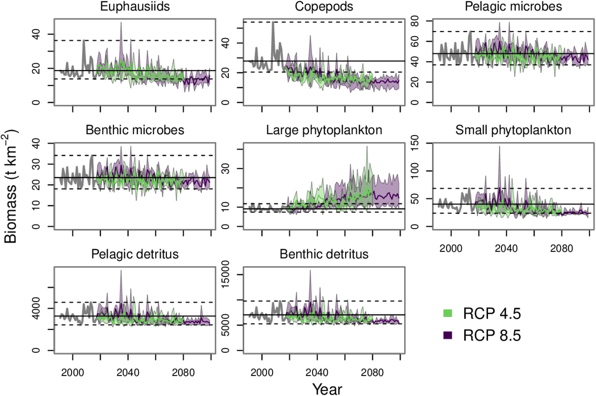
Figure 4. Annual mean biomass projections for pelagic and benthic detritus and the projections for the functional groups forced with outputs from lower trophic level modeling (euphausiids, copepods, pelagic microbes, benthic microbes, large phytoplankton, and small phytoplankton). The gray lines from 1991 to 2017 indicates the historical period. The purple and green polygons indicate the minimum and maximum range for the three earth system models run under each RCP. The purple and green lines indicate the mean of the three runs for each RCP. The dashed lines indicate the minimum and maximum values from the historical period and the solid black line indicates the mean value from the historical period.

Core Species

Under both RCPs, there was a general decline in the biomass of core species by the end of the century to values that were near or below the lowest values during the hindcast period (1991–2017) (Figure 5). The trajectories were similar under the three fishing scenarios, but for some species, distinct from the no-fishing scenario. This was especially evident for Pacific cod and yellowfin sole, which were subject to high exploitation rates under the scenarios with fishing. When fishing was halted at the start of the simulation period (2018) the biomass trajectories of Pacific cod and yellowfin sole responded with sharp increases. In contrast, the quota for northern rock sole is typically set well below their ABC (Witherell, 1995; Wilderbuer et al., 2019) and their biomass trajectory showed little change in response to the halting of fishing.

FIGURE 5

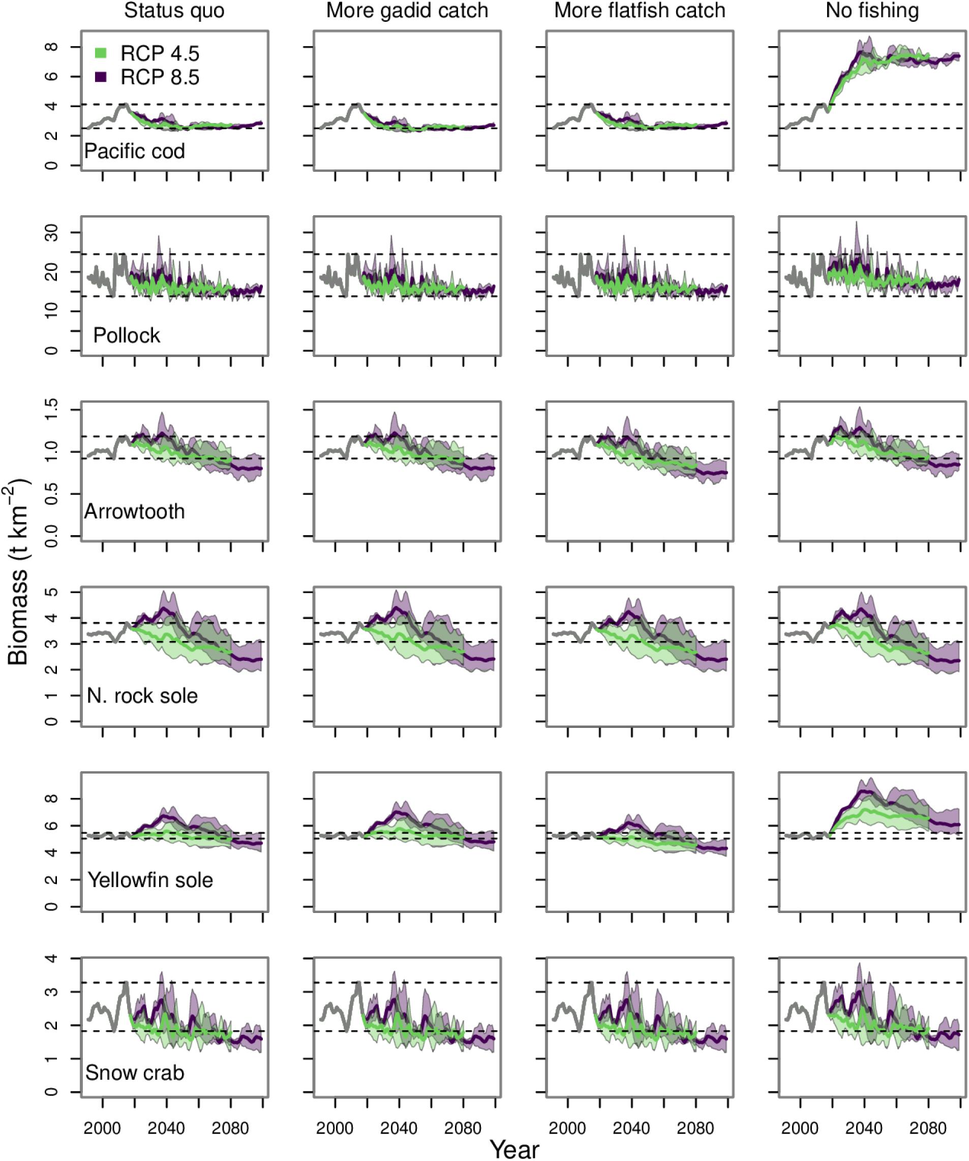
Figure 5. Biomass projections for the core commercial species run under all four fishing scenarios. The gray lines from 1991 to 2017 indicates the historical period. The purple and green polygons indicate the minimum and maximum range for the three earth system models run under each RCP. The purple and green lines indicate the mean of the three runs for each RCP. The dashed lines indicate the minimum and maximum values from the historical period.

The forecasted core species biomasses were similar among emission scenarios, but there were some differences in transient dynamics (Figure 5). The largest differences between RCPs occurred over the period from 2025 to 2045. During this window, all core species showed biomass peaks under RCP 8.5. Additionally, the biomass trajectories generally tracked higher under RCP 8.5 than under RCP 4.5 during these years. This pattern is similar to the biomass peaks for phytoplankton and zooplankton groups from the lower trophic level modeling and the detritus pools under RCP 8.5, which are all near or above their hindcast mean values during this time window. By 2060, the gap between biomass trajectories under the two RCPs was narrowing and by 2080, they were virtually equivalent.

In general, there were only minor differences in catch for most of the core species under the three fishing scenarios that included catch (Figure 6). Under the gadid preference scenario, the catch of pollock and Pacific cod was slightly higher than under the status quo scenario. Pollock catch declined gradually to values approximately equal to the lowest catches over the hindcast period under all three fishing scenarios. The catch of snow crab is highly variable but remains well above historical lows through the end of the century.

FIGURE 6

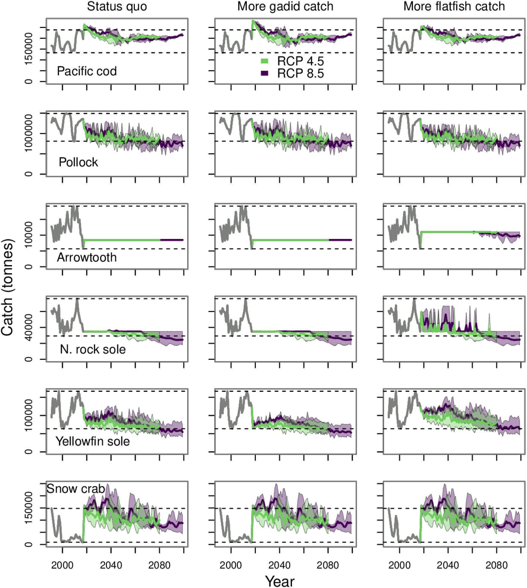
Figure 6. Catch projections for the core commercial species run under the three fishing scenarios that include fisheries catch. The gray line from 1991 to 2017 indicates the observed catch during the historical period. The purple and green polygons indicate the minimum and maximum range for the three earth system models run under each RCP. The purple and green lines indicate the mean of the three runs for each RCP. The dashed lines indicate the historical minimum and maximum values.

The catch of arrowtooth flounder, northern rock sole, and yellowfin sole were highest under the flatfish preference scenario (Figure 6). Northern rock sole had the most visible change in catch under the flatfish preference scenario. This was due to the reallocation of a portion of the catch originally allocated to gadids to flatfish, including northern rock sole. This reallocation of quota produced the sharp changes in northern rock sole catch under the flatfish preference scenario up through about mid-century. There was an increase in the arrowtooth flounder catch threshold under the flatfish preference; however, there were years toward the end of the century under RCP 8.5, where catch was below the threshold. This was because the biomass of arrowtooth flounder had dropped below their target biomass in those years and their ABC was on the “sloped” part of the harvest control rule. The catch of yellowfin sole declined through 2080 and the end of the century under all three fishing scenarios.

The catch trajectories for snow crab and Pacific cod had sharp changes in catch at the start of the projection period (2018, Figure 6). This was due to how we have simulated the harvest control rule. Our target exploitation rate was based on the status of the mass-balanced model during the base model time period (i.e., early 1990s). So long as their biomass was at or above their target biomass, these species would be subject to the target exploitation rate. In the case of snow crab and Pacific cod, this resulted in a jump in catch from the last year of the hindcast period (2017) to the start of the projection (2018). Additionally, the snow crab fishery is managed by the Alaska Department of Fish and Game and catch quotas are determined with a different harvest control rule than used in this study (NPFMC, 2020).

Marine Mammals and Seabirds

By 2080 the mean biomass trajectory for all marine mammal and seabird groups were below their minimum value from the hindcast period (Figures 7, 8). There were some increases in biomass under RCP 8.5 during the 2030s, but the trajectories declined thereafter. This pattern was due to fluctuations in prey abundance, which reflected the trajectories of the lower trophic level groups we have forced in these simulations. There were brief peaks in the biomass of phytoplankton, microbes, copepods, euphausiids, and detritus during the 2020s and 2030s under RCP 8.5 (Figure 4). These short-term increases by lower trophic level groups were transmitted up the food web to marine mammals and seabirds. Thereafter, the lower trophic level groups started to decline and the upper trophic level groups that fed upon them also started to decline. In particular, the decrease in copepods and euphausiids affected zooplanktivorous predators. For example, Auklets are particularly susceptible to declines in zooplankton as they depend on copepods and euphausiids for more than 80% of their base diet composition. The declines in zooplankton also drove declines in several forage fish species (e.g., herring, capelin, sandlance, and squid), many of which comprise large portions of the diet composition of piscivorous seabird and marine mammal groups.

FIGURE 7

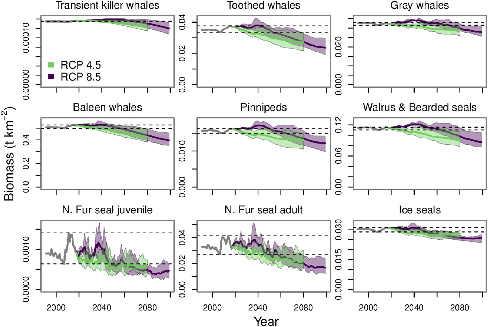
Figure 7. Biomass projections for marine mammal functional groups. The gray line from 1991 to 2017 indicates the historical period. The purple and green polygons indicate the minimum and maximum range for the three earth system models run under each RCP. The purple and green lines indicate the mean of the three runs for each RCP. The dashed lines indicate the minimum and maximum values from the historical period.

FIGURE 8

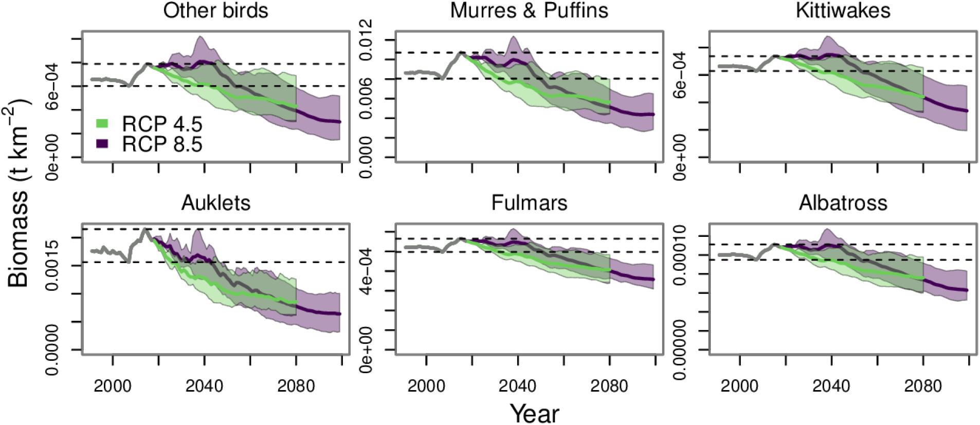
Figure 8. Biomass projections for seabird functional groups. The gray line from 1991 to 2017 indicates the historical period. The purple and green polygons indicate the minimum and maximum range for the three earth system models run under each RCP. The purple and green lines indicate the mean of the three runs for each RCP. The dashed lines indicate the minimum and maximum values from the historical period.

Trophic Guilds

The trophic guilds included all of the model’s functional groups, not just federally managed groundfish; therefore, we focused our results and discussion in this section on those projections run under the status quo and no fishing scenarios. Across all trophic guilds, RCPs and earth systems models, the food web model predicted declining biomass by 2080 and beyond if fishing was included (Figure 9). There was little observable difference in trophic guild biomass projections under the three fishing scenarios with catch (Supplementary Figure 2). Peak projected biomass values for all the guilds under RCP 8.5 were visible up to about mid-century. After that time, a decline in biomass was predicted, and by 2080, most of the trajectories under both RCPs were near the lowest values observed during the hindcast period.

FIGURE 9

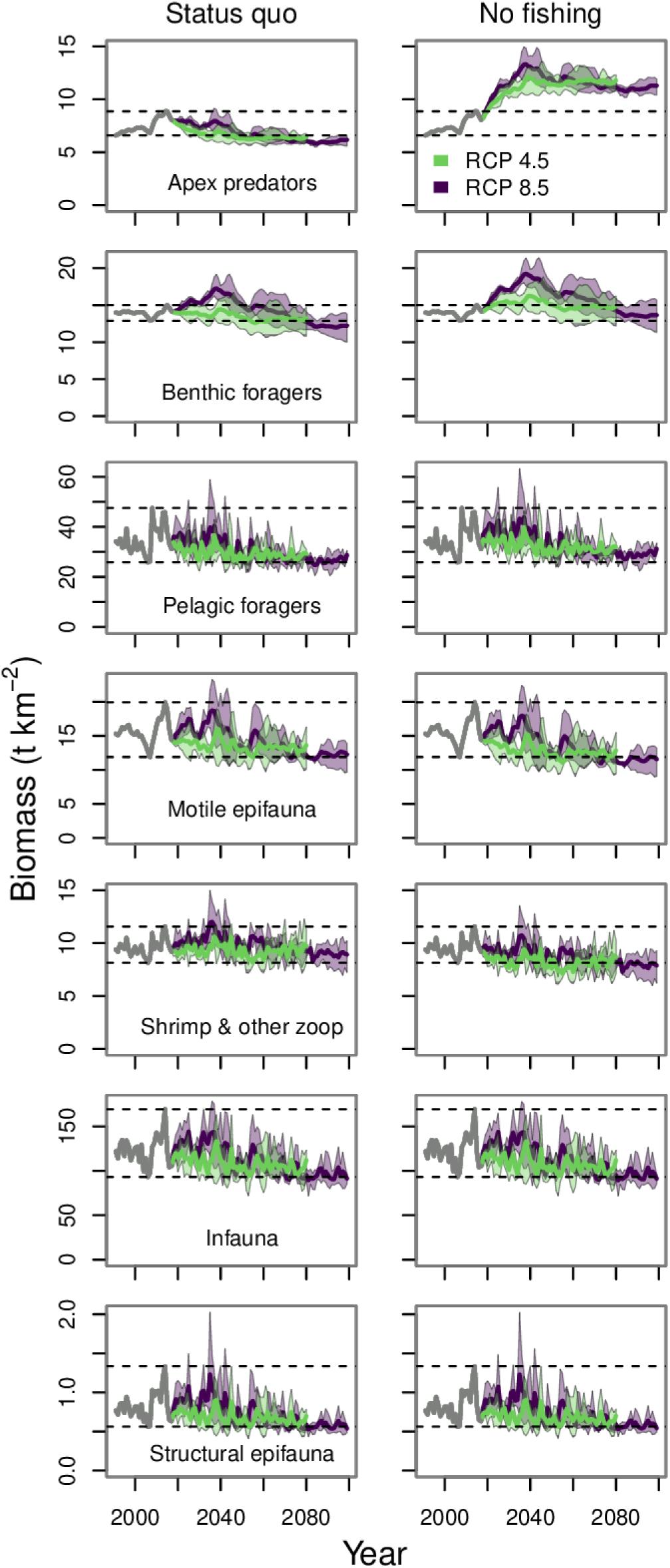
Figure 9. Biomass projections for trophic guilds under the status quo and no fishing scenarios. The gray lines from 1991 to 2017 indicates the historical period. The purple and green polygons indicate the minimum and maximum range for the three earth system models run under each RCP. The purple and green lines indicate the mean of the three runs for each RCP. The dashed lines indicate the minimum and maximum values from the historical period.

The motile epifauna, shrimp and other zooplankton, infauna, and structural epifauna guilds are dominated by invertebrates and showed little difference between the status quo and no fishing scenarios. The biomass trajectories for motile epifauna and the shrimp and other zooplankton guilds were slightly lower under the no fishing scenario. This was because several important predators of these guilds are commercial groundfish whose biomass, and thus consumption, increased under the no fishing scenario. The infauna and structural epifauna guilds are heavily dependent on primary production and detritus pools, and this was reflected in their biomass trajectories, the shape of which is similar to the projections for small phytoplankton and benthic and pelagic detritus (Figure 2).

All of the groundfish managed under the ecosystem cap are members of either the apex predators, benthic foragers, or pelagic foragers feeding guilds. The biomass dynamics of the apex predator guild were driven largely by Pacific cod, which are a biomass dominant component of this guild. The benthic foragers guild includes several flatfishes, including yellowfin sole and northern rock sole. These two flatfish species account for more than half of the total biomass of this guild and drive the guild dynamics. Similarly, the trajectory for the pelagic foragers guild was driven by pollock, which account for about half of the biomass of this guild.

For most functional groups within the apex predators, benthic foragers, motile epifauna, and pelagic foragers guilds there was a decline in biomass between the “present” and 2080 (Figure 10). However, some functional groups did increase in biomass. This occurred most frequently under the no fishing scenario. Within the apex guild, groups whose biomass increased over the simulation included Pacific cod (adults), skates, sharks, and Pacific halibut (Supplementary Figure 6). In the benthic foragers guild, Pacific cod juveniles, yellowfin sole, and Alaska plaice all experienced biomass increases under the no fishing scenario (Supplementary Figure 7). Among pelagic foragers, returning salmon, Pacific ocean perch, jellyfish, and other rockfish all experienced biomass increases under the no fishing scenario (Supplementary Figure 8). There were no scenario combinations where any groups within the motile epifauna guild experienced an increase in biomass (Supplementary Figure 9). The biomass projections for all remaining functional groups can be found in Supplementary Figures 10–12.

FIGURE 10

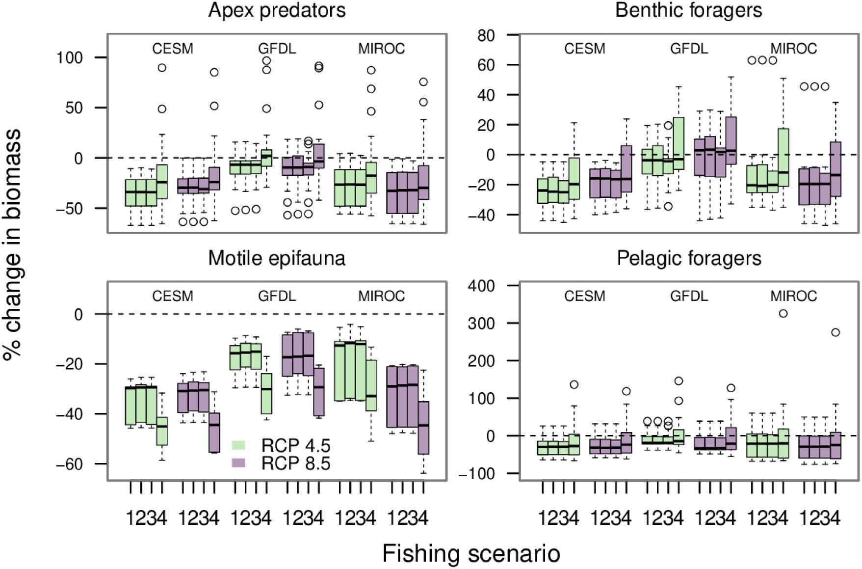
Figure 10. The percent change in biomass for functional groups between the end of the hindcast period (2008–2017) and the end of the projection period for the two RCPs (2071–2080). Each of the four panels is for one of the trophic guilds. Each box-and-whisker shows the percentage change in biomass for all the functional groups within the specified trophic guild by the earth system model-RCP-fishing scenario combination. The earth system models are labeled at the top of each panel. For each earth system model there are two RCPs, 4.5 is shown in green and 8.5 in purple. The fishing scenarios are labeled on the x-axis (1 = status quo, 2 = catch more gadids, 3 = catch more flatfish, 4 = no fishing). Outliers are shown with empty circles.

Within an earth system model-RCP combination, there was little difference in the outcomes between the three fishing scenarios that included catch (fishing scenarios 1–3 in Figure 10). The outcomes were generally higher for most groups within the apex predators, benthic foragers, and pelagic foragers guilds under the no fishing scenario (scenario 4 in Figure 10) than under the status quo scenario in each of the earth system model-RCP combinations. However, motile epifauna had generally lower biomass under the no fishing scenario. This was due to an increase in predation pressure from commercially fished predators whose biomass increased when there was no fishing.

Within each earth system model, and across these four trophic guilds, there was very little difference in the 2080 outcomes between the two RCPs, indicating that the differences between these climate-forcing scenarios did not sufficiently manifest themselves among the variables we used for climate forcing in this study. A greater distinction in 2080 outcomes is evident between the earth system models (Figure 10).

Sensitivity to Parameter Uncertainty

We generated 2.55 million Ecosim parameter sets for our sensitivity analysis, of which, 2,057 parameter sets survived the burn-in period and were retained for analysis. The distribution of biomass outcomes were wide for many functional groups. However, we found the median outcome, and 75% of the retained parameter sets, at the end of the century for the majority of functional groups to be in directional agreement with the simulations presented here (Supplementary Figure 4). The qualitative direction of change was in agreement with our simulations for most of the generated parameter sets.

Discussion

This work integrates multiple models to see how one mechanism—food web dynamics—might contribute to changes on population dynamics, community composition, and fishery catches under climate change. Our results indicate the bottom-up effects of projected climate change on the eastern Bering Sea could propagate through all levels of the food web, including marine mammals and seabirds. We found the biomass of most foraging guilds, individual species, and functional groups to decline gradually through 2080 under both RCP 4.5 and 8.5. The gradual declines predicted for primary (phytoplankton) and secondary producer biomass (zooplankton and microbes) drove declines in detritus pools, and ultimately were transmitted up the food web to all trophic levels, including commercially important groundfish and crabs. For some of the commercial groundfish species, increases in biomass by the end of the century could be realized under anticipated climate change when there was no fishing. This suggests that for some species the pressure from fisheries may be more significant than any negative pressure from the simulated climate forcing. Some commercial crab and benthic invertebrate groups had lower biomass when there was no fishing due to increased predation from commercial groundfish predators. By 2080, there was little distinction between the biomass trajectories subject to the high or intermediate emission scenarios for many of the groups, and a greater distinction in outcomes could be observed due to the earth system models. This indicates that by the end of the century the structural uncertainty in our simulations due to different earth system models was greater than the scenario uncertainty due to different emission pathways.

Fisheries can have a range of potential impacts on species and the ecosystem, and there is no single best way to forecast those impacts using a food web model. One approach commonly used with EwE models is to hold the fisheries mortality of targeted species at a constant value equal to present day fishing mortality, or held constant at a multiple of present day fishing mortality (e.g., Brown et al., 2010; Ainsworth et al., 2011; Niiranen et al., 2013; Bentley et al., 2017; Serpetti et al., 2017; Corrales et al., 2018; Fulton et al., 2018). However, neither of these scenarios mimic the actual way fisheries are managed in the eastern Bering Sea. Consequently, we incorporated a fisheries sub-model into our simulations that provided dynamic projections of annual catch quotas for US federally managed groundfish in the eastern Bering Sea in response to the changing status of managed stocks and in accordance with the existing fisheries management paradigm (Faig and Haynie, 2019). The constraint of the ecosystem harvest cap in the Bering Sea requires managers to consider social and economic tradeoffs when allocating quota under the cap. This leads to some stocks being fished well below the maximum sustainable fishing levels determined in stock assessments (Witherell et al., 2000). The fisheries sub-model predicted annual catch quotas given these cap-induced tradeoffs and region-specific management practices (Faig and Haynie, 2019).

The gradual declines in biomass for most species and functional groups in our projections of the eastern Bering Sea food web are in directional agreement with other regional and global multi-species modeling studies forecasting fish and total animal biomass through the end of the century. At high latitudes, in particular the Arctic Ocean, total animal biomass is predicted to increase due to a confluence of factors including increased primary production, warming temperatures, and poleward range expansions of productive, commercial, temperate species into the Arctic (Cheung et al., 2009; Fossheim et al., 2015; Lefort et al., 2015; Bryndum-Buchholz et al., 2019; Lotze et al., 2019). At lower latitudes, global projections are less decisive and there are mixed outcomes that may vary according to structural, scenario, and parameter uncertainty (Lotze et al., 2019). In comparison to global models that include projected total biomass declines in the eastern Bering Sea (Bryndum-Buchholz et al., 2019; Lotze et al., 2019), the declines we projected in this study are modest, and the range of uncertainty in our simulations allows for the maintenance of biomass for many species, or in some cases an increase in biomass.

The biomass declines we projected for many species are smaller in magnitude, in part, due to how we implemented climate forcing in our study and the absence of some other climate-related processes and direct effects that would influence the future trajectories of species. Previous studies in other regions have simulated the effects of anticipated climate change using EwE models by forcing the production rate of phytoplankton to be consistent with projections from earth system models (Brown et al., 2010; Ainsworth et al., 2011; Howell et al., 2013; Niiranen et al., 2013; Watson et al., 2013; Suprenand and Ainsworth, 2017; Fulton et al., 2018; Ehrnsten et al., 2019), or by scaling predator consumption by their thermal tolerance and forecasted temperature change (Bentley et al., 2017; Serpetti et al., 2017; Corrales et al., 2018), or by scaling reproductive output to climate forecasts (Niiranen et al., 2013; Ehrnsten et al., 2019). Alternatively, we have linked our food web model to a climate-enhanced regional ocean and biogeochemical model to represent the biomass dynamics of key lower trophic level groups. By fixing the biomass trajectories of these lower trophic level groups in this manner, their biomass dynamics are not subject to top–down pressure. Our results are strictly limited to the bottom-up effects of forecasted reductions in primary and secondary producer biomass on the food web, as mediated by the network of trophic interactions. Including the direct physiological effects of temperature in future simulation studies could result in more pronounced declines for species when temperatures exceed their thermal envelopes, and more pronounced increases in biomass for species with a higher thermal tolerance who can take advantage of the changing conditions.

The biomass and catch trajectories from our model are limited projections of potential climate impacts in the eastern Bering Sea as they are constrained by the processes represented in our food web model and to the nature of climate forcing used in our simulations. The outputs from the Bering10K model used to simulate climate forcing integrate the direct effects of temperature and other biophysical forces on those lower trophic levels (Gibson and Spitz, 2011; Hermann et al., 2019). For example, the BESTNPZ model included temperature-dependent mortality of large zooplankton, as a proxy for temperature-dependent predation. However, our food web model does not explicitly consider the direct biophysical effects of climate change on the remainder of the food web. Temperature will directly impact the physiology, behavior, and performance of ectotherms (Portner and Peck, 2010), drive species distribution shifts (Mueter and Litzow, 2008; Frainer et al., 2017; Stevenson and Lauth, 2019), and facilitate the introduction of non-indigenous species from warmer regions (Cheung et al., 2015; Alabia et al., 2018; Droghini et al., 2020). We did not examine the direct effects of climate change on physiological processes in this study and leave that for future work.

The direct physiological effects of temperature may attenuate or accentuate the indirect effects of climate change represented in our food web model. Methods to incorporate the direct effects of temperature on organisms have been developed for EwE (e.g., Bentley et al., 2017; Serpetti et al., 2017) but similar methods have not yet been developed for Rpath. The biological reference points we used with our harvest control rules are rooted in the static, mass-balanced model configuration and the environmental conditions of the base model time-period of the early 1990s. Under the projected environmental conditions those biological reference points (e.g., target biomass) may no longer be valid in the future and updated values should be calculated to reflect the stock’s current productivity (Haltuch et al., 2009). Other considerations for future simulations include the effects of ocean acidification, deoxygenation, loss of habitat (e.g., sea ice), and emigration or invasion of new species from adjacent regions.

The declines in biomass across most groups in the eastern Bering Sea through the end of the century in our study are similar to the findings of other climate-enhanced multi-species models from the ACLIM project. Reum et al. (2020) used a multi-species size-spectrum model to make biomass projections of the eastern Bering Sea food web and found on average that spawning stock biomass for the groundfish community declined through the end of the century. However, they found the direction of trend in biomass among several groundfish species did not agree across all climate change scenarios. Holsman et al. (2020) used a multi-species statistical catch-at-age model to make projections for pollock, Pacific cod, and arrowtooth flounder through the end of the century and similarly observed declining biomass for all three species under RCPs 4.5 and 8.5. A key distinction between our simulations and those of Holsman et al. (2020) and Reum et al. (2020) is that we did not include the direct effects of temperature on biological processes and instead focused on the impacts of climate-induced changes at lower trophic levels on the whole food web. The declines in biomass that we observed for pollock and Pacific cod in our simulations are minor in comparison to these other two studies, and in the case of arrowtooth flounder, are not in directional agreement with Reum et al. (2020). The more comprehensive network of trophic interactions in our Rpath model provides additional detail on trophic interactions across the whole food web but lacks the physiological detail of temperature effects included in these other two studies. Additionally, there are many other differences in the structural assumptions made by these modeling frameworks, which may contribute substantially to projection results differing in direction or magnitude (Jacobsen et al., 2016). The structural differences between the suite of biological models included in the ACLIM project are an advantage of the multi-model ensemble approach, and these differences will be utilized in future work to help quantify structural uncertainty in ensemble projections (Hollowed et al., 2020).

Uncertainty in our projections is present at multiple levels of the modeling hierarchy and should be taken into consideration when interpreting the results. The outputs of our simulations are quantitative, and it is tempting to view the trajectories as accurate or precise projections. However, they stem from a single model configuration and are subject to initialization and parameter uncertainty, in addition to scenario and structural uncertainty (Payne et al., 2016). Knowledge of forecasts and projections can potentially influence the decision-making process, therefore it is important that simulation results are viewed in the appropriate context (Hobday et al., 2019). Our projections are best interpreted in a qualitative manner, in terms of the direction of change and the agreement across simulation scenarios (Ainsworth et al., 2011).

Our use of multiple climate and fishing scenarios is a start to addressing scenario uncertainty but only accounts for a limited portion of this uncertainty. Scenario uncertainty is due to an inability to know what the full potential range of future outcomes includes. RCPs 8.5 and 4.5 represent upper and intermediate levels of warming, respectively, among the RCPs available, but we did not include RCP 2.6 in our modeling framework (Hollowed et al., 2020), which is a pathway with high levels of mitigation and low greenhouse gas emissions. Including the lowest emission scenario may have provided additional contrast in the outcomes and revealed interactions between fisheries and climate that were not present in our current simulations, and would have presented a broader picture of scenario uncertainty due to climate.

Our fisheries scenarios are rooted in the existing fisheries management paradigm and historical management decisions. Thus, they do not reflect conditions that exist outside the historical record and cannot predict how future management decisions under unprecedented conditions may differ from historical practices. The portion of scenario uncertainty due to human responses to unforeseen or unprecedented conditions is irreducible in many respects, and will likely always be present to some degree in any future projections (Hawkins et al., 2016; Payne et al., 2016; Planque, 2016).

Structural uncertainty is due to a limited understanding of the processes and mechanisms that determine population and ecosystem dynamics and are represented with simplified processes in models. To help address structural uncertainty, we used three earth system models to project future climate. The importance of structural uncertainty can be seen in our projection outcomes at 2080, where a greater distinction in outcomes is seen between earth system models as opposed to between the two RCPs (Figure 10). This outcome emphasizes the importance of using multiple earth system models in climate projections with biological models, and highlights how important the selected earth system models can be in determining the end of century outcomes. Frölicher et al. (2016) found that most uncertainty in century-scale projections of net primary production with earth system models was attributed to structural uncertainty, followed by scenario uncertainty. This result is similar to the findings of Reum et al. (2020) who observed that uncertainty in projections with a multi-species size-spectrum model up to mid-century was primarily due to the climate scenario, but thereafter it was primarily due to the earth system model.

The total uncertainty in our Rpath projections also includes the uncertainty present in the earth system models and the oceanographic and lower trophic level modeling, whose outputs drive our projections. The uncertainty in previous steps in the model hierarchy accumulates in our model, adding to the total uncertainty (Payne et al., 2016). An additional source of structural uncertainty in the ACLIM modeling framework is the use of a single ocean and biogeochemical model. The Bering10K model provides the biological indices used to simulate climate forcing in our Rpath projections. While the Bering 10K outputs have demonstrated skill at projecting physical, thermal, and nutrient dynamics, room for improvement remains with the skill of reproducing primary and secondary production group dynamics (Kearney et al., 2020). We acknowledge that these biological variables with lower skill are those variables we are using to simulate climate change within our Rpath model.

The risk of climate change impacts on the eastern Bering Sea food web persists under both the business-as-usual (RCP 8.5) and the moderate emission scenario (RCP 4.5). The best way to limit the impacts of climate change on marine ecosystems and fisheries is to reduce greenhouse gas emissions (Cheung et al., 2016; Gattuso et al., 2018). In the face of climate change impacts, the long-term sustainability of fisheries can be best ensured with effective ecosystem-based fisheries management that is responsive to the impacts of climate change on species and the food web (Gaines et al., 2018; Fulton et al., 2019; Free et al., 2020; Holsman et al., 2020). Our climate-enhanced projections with Rpath can support fisheries managers by contributing to an improved understanding of the long-term effects of forecasted climate change on commercial and non-commercial species, and in consideration of region-specific policies and tradeoffs confronting fisheries managers. We incorporated a fisheries sub-model that could emulate region-specific management practices and make dynamic catch predictions during the simulations, which provided additional detail over the alternative of using a constant multiplier of present day fishing mortality. Our model projections are one part of a larger ensemble of biological models in the ACLIM project that will be jointly considered in future work to quantify different sources of uncertainty and provide a more comprehensive suite of future projections for the eastern Bering Sea (Hollowed et al., 2020). While our Rpath projections are not suited to inform tactical management decisions, as they do not include adequate measures of uncertainty or the likelihood of different outcomes, our method for incorporating climate and fisheries into food web projections can serve as a starting point for future studies that consider additional climate stressors and more comprehensive accounting of uncertainty.

Data Availability Statement

The datasets generated for this study and the food web model files are available on request to the corresponding author.

Author Contributions

GW, KA, ABH, and KH conceived of the study. WC and AJH provided downscaled climate projections. KK, KA, and KH provided lower trophic level modeling. AF and ACH provided code and text for the fisheries scenarios. GW and KA developed the simulation design and model code. GW conducted the simulations and analysis. KA, ABH, AP, and TE provided oversight and mentorship to GW. ABH, KH, KA, ACH, AJH, and AP acquired funding. GW wrote the original manuscript draft. All authors provided critical revision of the manuscript and approved of the submitted version.

Funding

Multiple NOAA National Marine Fisheries programs provided support for ACLIM including Fisheries and the Environment (FATE), Stock Assessment Analytical Methods (SAAM) Science and Technology North Pacific Climate Regimes and Ecosystem Productivity, the Integrated Ecosystem Assessment Program (IEA), NOAA Research Transition Acceleration Program (RTAP), the Alaska Fisheries Science Center (ASFC), the Office of Oceanic and Atmospheric Research (OAR), and the National Marine Fisheries Service (NMFS). GW received funding from the ROK-USA Joint Project Agreement Fisheries Panel. This study was funded in part by the NOAA Integrated Ecosystem Assessment Program, Contribution No. 2020_4. This publication is partially funded by the Joint Institute for the Study of the Atmosphere and Ocean (JISAO) under NOAA Cooperative Agreement No. NA15OAR4320063, Contribution No. 2020-1085.

Conflict of Interest

The authors declare that the research was conducted in the absence of any commercial or financial relationships that could be construed as a potential conflict of interest.

Acknowledgments

We would like to thank the entire ACLIM team including J. Ianelli, S. Kasperski, P. Spencer, J. Reum, C. Stawitz, W. Stockhausen, C. Szuwalski, and T. Wilderbuer for feedback and discussions on the broader application of this work. We thank S. Rohan and J. Reum for reviewing an earlier version of this manuscript. We also thank the journal reviewers for their helpful reviews and comments. Thanks to G. M. Lang for the map of the study area. The scientific views, opinions, and conclusions expressed herein are solely those of the authors and do not represent the views, opinions, or conclusions of NOAA or the U.S. Department of Commerce.

Supplementary Material

The Supplementary Material for this article can be found online at: https://www.frontiersin.org/articles/10.3389/fmars.2021.624301/full#supplementary-material

Footnotes

1. ^ ecopath.org
2. ^ https://github.com/NOAA-EDAB/Rpath

References

Ainsworth, C. H., Samhouri, J. F., Busch, D. S., Cheung, W. W. L., Dunne, J., and Okey, T. A. (2011). Potential impacts of climate change on Northeast Pacific marine foodwebs and fisheries. ICES J. Mar. Sci. 68, 1217–1229. doi: 10.1093/icesjms/fsr043

CrossRef Full Text | Google Scholar

Alabia, I. D., Molinos, J. G., Saitoh, S. I., Hirawake, T., Hirata, T., and Mueter, F. J. (2018). Distribution shifts of marine taxa in the Pacific Arctic under contemporary climate changes. Divers Distrib. 24, 1583–1597. doi: 10.1111/ddi.12788

CrossRef Full Text | Google Scholar

Allison, E. H., and Bassett, H. R. (2015). Climate change in the oceans: human impacts and responses. Science 350, 778–782. doi: 10.1126/science.aac8721

PubMed Abstract | CrossRef Full Text | Google Scholar

Anderson, C. N. K., Hsieh, C. H., Sandin, S. A., Hewitt, R., Hollowed, A., Beddington, J., et al. (2008). Why fishing magnifies fluctuations in fish abundance. Nature 452, 835–839. doi: 10.1038/nature06851

PubMed Abstract | CrossRef Full Text | Google Scholar

Aydin, K. Y., Gaichas, S., Ortiz, I., Kinzey, D., and Friday, N. (2007). A Comparison of the Bering Sea, Gulf of Alaska, and Aleutian Islands large Marine Ecosystems through Food Web Modeling. U.S. Dep. Commer. NOAA Tech Memo NMFS-AFSC-178. Washington, DC: NOAA.

Google Scholar

Baker, M. R., Kivva, K. K., Pisareva, M. N., Watson, J. T., and Selivanova, J. (2020). Shifts in the physical environment in the Pacific Arctic and implications for ecological timing and conditions. Deep Sea Res. II. Top. Stud. Oceanogr. 177:104802. doi: 10.1016/j.dsr2.2020.104802

CrossRef Full Text | Google Scholar

Bentley, J. W., Serpetti, N., and Heymans, J. J. (2017). Investigating the potential impacts of ocean warming on the Norwegian and Barents Seas ecosystem using a time-dynamic food-web model. Ecol. Model 360, 94–107. doi: 10.1016/j.ecolmodel.2017.07.002

CrossRef Full Text | Google Scholar

Berkeley, S. A., Hixon, M. A., Larson, R. J., and Love, M. S. (2004). Fisheries Sustainability via protection of age structure and spatial distribution of fish populations. Fisheries 29, 23–32.

Google Scholar

Bopp, L., Resplandy, L., Orr, J. C., Doney, S. C., Dunne, J. P., Gehlen, M., et al. (2013). Multiple stressors of ocean ecosystems in the 21st century: projections with CMIP5 models. Biogeosciences 10, 6225–6245. doi: 10.5194/bg-10-6225-2013

CrossRef Full Text | Google Scholar

Boyce, D. G., and Worm, B. (2015). Patterns and ecological implications of historical marine phytoplankton change. Mar. Ecol. Prog. Ser. 534, 251–272. doi: 10.3354/meps11411

CrossRef Full Text | Google Scholar

Brown, C. J., Fulton, E. A., Hobday, A. J., Matear, R. J., Possingham, H. P., Bulman, C., et al. (2010). Effects of climate-driven primary production change on marine food webs: implications for fisheries and conservation. Glob. Change Biol. 16, 1194–1212. doi: 10.1111/j.1365-2486.2009.02046.x

CrossRef Full Text | Google Scholar

Bryndum-Buchholz, A., Tittensor, D. P., Blanchard, J. L., Cheung, W. W. L., Coll, M., Galbraith, E. D., et al. (2019). Twenty-first-century climate change impacts on marine animal biomass and ecosystem structure across ocean basins. Glob. Change Biol. 25, 459–472. doi: 10.1111/gcb.14512

PubMed Abstract | CrossRef Full Text | Google Scholar

Cahalan, J., Gasper, J., and Mondragon, J. (2014). Catch Sampling and Estimation in the Federal Groundfish Fisheries off Alaska, 2015 edition. U.S. Dep. Commer., NOAA Tech Memo NMFS-AFSC-286. Washington, DC: NOAA.

Google Scholar

Chassot, E., Bonhommeau, S., Dulvy, N. K., Melin, F., Watson, R., Gascuel, D., et al. (2010). Global marine primary production constrains fisheries catches. Ecol. Lett. 13, 495–505. doi: 10.1111/j.1461-0248.2010.01443.x

PubMed Abstract | CrossRef Full Text | Google Scholar

Cheng, L. J., Abraham, J., Hausfather, Z., and Trenberth, K. E. (2019). How fast are the oceans warming? Science 363, 128–129. doi: 10.1126/science.aav7619

PubMed Abstract | CrossRef Full Text | Google Scholar

Cheung, W. W. L., Brodeur, R. D., Okey, T. A., and Pauly, D. (2015). Projecting future changes in distributions of pelagic fish species of Northeast Pacific shelf seas. Prog. Oceanogr. 130, 19–31. doi: 10.1016/j.pocean.2014.09.003

CrossRef Full Text | Google Scholar

Cheung, W. W. L., Lam, V. W. Y., Sarmiento, J. L., Kearney, K., Watson, R., and Pauly, D. (2009). Projecting global marine biodiversity impacts under climate change scenarios. Fish Fish. 10, 235–251. doi: 10.1111/j.1467-2979.2008.00315.x

CrossRef Full Text | Google Scholar

Cheung, W. W. L., Reygondeau, G., and Frölicher, T. L. (2016). Large benefits to marine fisheries of meeting the 1.5 degrees C global warming target. Science 354, 1591–1594. doi: 10.1126/science.aag2331

PubMed Abstract | CrossRef Full Text | Google Scholar

Christensen, V., and Pauly, D. (1992). Ecopath II-a software for balancing steady-state ecosystem models and calculating network characteristics. Ecol. Model 61, 169–185. doi: 10.1016/0304-3800(92)90016-8

CrossRef Full Text | Google Scholar

Christensen, V., and Walters, C. J. (2004). Ecopath with ecosim: methods, capabilities and limitations. Ecol. Model 172, 109–139. doi: 10.1016/j.ecolmodel.2003.09.003

CrossRef Full Text | Google Scholar

Citta, J. J., Lowry, L. F., Quakenbush, L. T., Kelly, B. P., Fischbach, A. S., London, J. M., et al. (2018). A multi-species synthesis of satellite telemetry data in the Pacific Arctic (1987-2015): overlap of marine mammal distributions and core use areas. Deep Sea Res. II Top. Stud. Oceanogr. 152, 132–153. doi: 10.1016/j.dsr2.2018.02.006

CrossRef Full Text | Google Scholar

Coachman, L. K. (1986). Circulation, water masses, and fluxes on the southeastern Bering Sea shelf. Cont. Shelf Res. 5, 23–108. doi: 10.1016/0278-4343(86)90011-7

CrossRef Full Text | Google Scholar

Cooper, D., Rogers, L. A., and Wilderbuer, T. (2020). Environmentally driven forecasts of northern rock sole (Lepidopsetta polyxystra) recruitment in the eastern Bering Sea. Fish Oceanogr. 29, 111–121. doi: 10.1111/fog.12458

CrossRef Full Text | Google Scholar

Cooper, L. W., Sexson, M. G., Grebmeier, J. M., Gradinger, R., Mordy, C. W., and Lovvorn, J. R. (2013). Linkages between sea-ice coverage, pelagic-benthic coupling, and the distribution of spectacled eiders: observations in March 2008, 2009 and 2010, northern Bering Sea. Deep Sea Res. II Top. Stud. Oceanogr. 94, 31–43. doi: 10.1016/j.dsr2.2013.03.009

CrossRef Full Text | Google Scholar

Corrales, X., Coll, M., Ofir, E., Heymans, J. J., Steenbeek, J., Goren, M., et al. (2018). Future scenarios of marine resources and ecosystem conditions in the Eastern Mediterranean under the impacts of fishing, alien species and sea warming. Sci. Rep. 8:16. doi: 10.1038/s41598-018-32666-x

PubMed Abstract | CrossRef Full Text | Google Scholar

Coyle, K. O., Eisner, L. B., Mueter, F. J., Pinchuk, A. I., Janout, M. A., Cieciel, K. D., et al. (2011). Climate change in the southeastern Bering Sea: impacts on pollock stocks and implications for the oscillating control hypothesis. Fish Oceanogr. 20, 139–156. doi: 10.1111/j.1365-2419.2011.00574.x

CrossRef Full Text | Google Scholar

Coyle, K. O., and Gibson, G. A. (2017). Calanus on the Bering Sea shelf: probable cause for population declines during warm years. J. Plankton Res. 39, 257–270. doi: 10.1093/plankt/fbx005

PubMed Abstract | CrossRef Full Text | Google Scholar

Danielson, S. L., Ahkinga, O., Ashjian, C., Basyuk, E., Cooper, L. W., Eisner, L., et al. (2020). Manifestation and consequences of warming and altered heat fluxes over the bering and Chukchi Sea continental shelves. Deep Sea Res. II Top. Stud. Oceanogr. 177:104781. doi: 10.1016/j.dsr2.2020.104781

CrossRef Full Text | Google Scholar

Doney, S. C., Ruckelshaus, M., Emmett Duffy, J., Barry, J. P., Chan, F., English, C. A., et al. (2012). Climate change impacts on marine ecosystems. Ann. Rev. Mar. Sci. 4, 11–37.

Google Scholar

Droghini, A., Fischbach, A. S., Watson, J. T., and Reimer, J. P. (2020). Regional ocean models indicate changing limits to biological invasions in the Bering Sea. ICES J. Mar. Sci. 77, 964–974. doi: 10.1093/icesjms/fsaa014

CrossRef Full Text | Google Scholar

Duffy-Anderson, J. T., Barbeaux, S. J., Farley, E., Heintz, R., Horne, J. K., Parker-Stetter, S. L., et al. (2016). The critical first year of life of walleye pollock (Gadus chalcogrammus) in the eastern Bering Sea: implications for recruitment and future research. Deep Sea Res. II Top. Stud. Oceanogr. 134, 283–301. doi: 10.1016/j.dsr2.2015.02.001

CrossRef Full Text | Google Scholar

Duffy-Anderson, J. T., Stabeno, P., Andrews, A. G., Cieciel, K., Deary, A., Farley, E., et al. (2019). Responses of the northern Bering Sea and southeastern Bering Sea pelagic ecosystems following record-breaking low winter sea ice. Geophys. Res. Lett. 46, 9833–9842. doi: 10.1029/2019gl083396

CrossRef Full Text | Google Scholar

Dunne, J. P., John, J. G., Adcroft, A. J., Griffies, S. M., Hallberg, R. W., Shevliakova, E., et al. (2012). GFDL’s ESM2 global coupled climate-carbon Earth system models. Part I: physical formulation and baseline simulation characteristics. J. Climate 25, 6646–6665. doi: 10.1175/jcli-d-11-00560.1

CrossRef Full Text | Google Scholar

Ehrnsten, E., Bauer, B., and Gustafsson, B. G. (2019). Combined effects of environmental drivers on marine trophic groups - a systematic model comparison. Front. Mar. Sci. 6:14. doi: 10.3389/fmars.2019.00492

CrossRef Full Text | Google Scholar

Eisner, L. B., Pinchuk, A. I., Kimmel, D. G., Mier, K. L., Harpold, C. E., and Siddon, E. C. (2018). Seasonal, interannual, and spatial patterns of community composition over the eastern Bering Sea shelf in cold years. Part I: zooplankton. ICES J. Mar. Sci. 75, 72–86. doi: 10.1093/icesjms/fsx156

CrossRef Full Text | Google Scholar

Faig, A., and Haynie, A. C. (2019). catchfunction: BSAI Catch Function. R Package Version 1.5.3.

Google Scholar

FAO (2019). FAO Yearbook. Fishery and Aquaculture Statistics 2017. Rome: FAO.

Google Scholar

Farley, E. V., Heintz, R. A., Andrews, A. G., and Hurst, T. P. (2016). Size, diet, and condition of age-0 Pacific cod (Gadus macrocephalus) during warm and cool climate states in the eastern Bering sea. Deep Sea Res. II Top. Stud. Oceanogr. 134, 247–254. doi: 10.1016/j.dsr2.2014.12.011

CrossRef Full Text | Google Scholar

Fissel, B., Dalton, M., Garber-Yonts, B., Haynie, A., Kasperski, S., Lee, J., et al. (2017). Stock Assessment and Fishery Evaluation Report for the Groundfish Fisheries of the Gulf of Alaska and Bering Sea/Aleutian Islands Area: Economic Status of the Groundfish Fisheries off Alaska, 2016. Anchorage, AK: North Pacific Fishery Management Council.

Google Scholar

Fossheim, M., Primicerio, R., Johannesen, E., Ingvaldsen, R. B., Aschan, M. M., and Dolgov, A. V. (2015). Recent warming leads to a rapid borealization of fish communities in the Arctic. Nat. Clim. Change 5, 673–677. doi: 10.1038/nclimate2647

CrossRef Full Text | Google Scholar

Frainer, A., Primicerio, R., Kortsch, S., Aune, M., Dolgov, A. V., Fossheim, M., et al. (2017). Climate-driven changes in functional biogeography of Arctic marine fish communities. Proc. Natl. Acad. Sci. U.S.A. 114, 12202–12207. doi: 10.1073/pnas.1706080114

PubMed Abstract | CrossRef Full Text | Google Scholar

Free, C. M., Mangin, T., Molinos, J. G., Ojea, E., Burden, M., Costello, C., et al. (2020). Realistic fisheries management reforms could mitigate the impacts of climate change in most countries. PLoS One 15:21. doi: 10.1371/journal.pone.0224347

PubMed Abstract | CrossRef Full Text | Google Scholar

Frölicher, T. L., Rodgers, K. B., Stock, C. A., and Cheung, W. W. L. (2016). Sources of uncertainties in 21st century projections of potential ocean ecosystem stressors. Glob. Biogeochem. Cycle 30, 1224–1243. doi: 10.1002/2015gb005338

CrossRef Full Text | Google Scholar

Fulton, E. A., Bulman, C. M., Pethybridge, H., and Goldsworthy, S. D. (2018). Modelling the great Australian bight ecosystem. Deep Sea Res. II Top. Stud. Oceanogr. 157, 211–235. doi: 10.1016/j.dsr2.2018.11.002

CrossRef Full Text | Google Scholar

Fulton, E. A., Punt, A. E., Dichmont, C. M., Harvey, C. J., and Gorton, R. (2019). Ecosystems say good management pays off. Fish Fish. 20, 66–96. doi: 10.1111/faf.12324

CrossRef Full Text | Google Scholar

Gadamus, L., and Raymond-Yakoubian, J. (2015). A bering strait indigenous framework for resource management: respectful seal and walrus hunting. Arct. Anthropol. 52, 87–101. doi: 10.3368/aa.52.2.87

CrossRef Full Text | Google Scholar

Gaichas, S. K., Odell, G., Aydin, K. Y., and Francis, R. C. (2012). Beyond the defaults: functional response parameter space and ecosystem-level fishing thresholds in dynamic food web model simulations. Can. J. Fish. Aquat. Sci. 69, 2077–2094. doi: 10.1139/f2012-099

CrossRef Full Text | Google Scholar

Gaines, S. D., Costello, C., Owashi, B., Mangin, T., Bone, J., Molinos, J. G., et al. (2018). Improved fisheries management could offset many negative effects of climate change. Sci. Adv. 4:8. doi: 10.1126/sciadv.aao1378

PubMed Abstract | CrossRef Full Text | Google Scholar

Gattuso, J. P., Magnan, A. K., Bopp, L., Cheung, W. W. L., Duarte, C. M., Hinkel, J., et al. (2018). Ocean solutions to address climate change and its effects on marine ecosystems. Front. Mar. Sci. 5:18. doi: 10.3389/fmars.2018.00337

CrossRef Full Text | Google Scholar

Gibson, G. A., and Spitz, Y. H. (2011). Impacts of biological parameterization, initial conditions, and environmental forcing on parameter sensitivity and uncertainty in a marine ecosystem model for the Bering Sea. J. Mar. Syst. 88, 214–231. doi: 10.1016/j.jmarsys.2011.04.008

CrossRef Full Text | Google Scholar

Grebmeier, J. M., Overland, J. E., Moore, S. E., Farley, E. V., Carmack, E. C., Cooper, L. W., et al. (2006). A major ecosystem shift in the northern Bering Sea. Science 311, 1461–1464. doi: 10.1126/science.1121365

PubMed Abstract | CrossRef Full Text | Google Scholar

Haltuch, M. A., Punt, A. E., and Dorn, M. W. (2009). Evaluating the estimation of fishery management reference points in a variable environment. Fish. Res. 100, 42–56. doi: 10.1016/j.fishres.2009.03.001

CrossRef Full Text | Google Scholar

Hawkins, E., Osborne, T. M., Ho, C. K., and Challinor, A. J. (2013). Calibration and bias correction of climate projections for crop modelling: an idealised case study over Europe. Agr. For. Meteorol. 170, 19–31. doi: 10.1016/j.agrformet.2012.04.007

CrossRef Full Text | Google Scholar

Hawkins, E., Smith, R. S., Gregory, J. M., and Stainforth, D. A. (2016). Irreducible uncertainty in near-term climate projections. Clim. Dyn. 46, 3807–3819. doi: 10.1007/s00382-015-2806-8

CrossRef Full Text | Google Scholar

Hermann, A. J., Gibson, G. A., Bond, N. A., Curchitser, E. N., Hedstrom, K., Cheng, W., et al. (2016). Projected future biophysical states of the Bering Sea. Deep Sea Res. II Top. Stud. Oceanogr. 134, 30–47. doi: 10.1016/j.dsr2.2015.11.001

CrossRef Full Text | Google Scholar

Hermann, A. J., Gibson, G. A., Bond, N. A., Curchitser, E. N., Hedstrom, K., Cheng, W., et al. (2013). A multivariate analysis of observed and modeled biophysical variability on the Bering Sea shelf: multidecadal hindcasts (1970-2009) and forecasts (2010-2040). Deep Sea Res II Top. Stud. Oceanogr. 94, 121–139. doi: 10.1016/j.dsr2.2013.04.007

CrossRef Full Text | Google Scholar

Hermann, A. J., Gibson, G. A., Cheng, W., Ortiz, I., Aydin, K., Wang, M., et al. (2019). Projected biophysical conditions of the Bering Sea to 2100 under multiple emission scenarios. ICES J. Mar. Sci. 76, 1280–1304. doi: 10.1093/icesjms/fsz043

CrossRef Full Text | Google Scholar

Hidalgo, M., Rouyer, T., Molinero, J. C., Massuti, E., Moranta, J., Guijarro, B., et al. (2011). Synergistic effects of fishing-induced demographic changes and climate variation on fish population dynamics. Mar. Ecol. Prog. Ser. 426, 1–12. doi: 10.3354/meps09077

CrossRef Full Text | Google Scholar

Ho, C. K., Stephenson, D. B., Collins, M., Ferro, C. A. T., and Brown, S. J. (2012). Calibration strategies a source of additional uncertainty in climate change projections. Bull. Am. Meteorol. Soc. 93, 21–26. doi: 10.1175/2011bams3110.1

CrossRef Full Text | Google Scholar

Hobday, A. J., Hartog, J. R., Manderson, J. P., Mills, K. E., Oliver, M. J., Pershing, A. J., et al. (2019). Ethical considerations and unanticipated consequences associated with ecological forecasting for marine resources. ICES J. Mar. Sci. 76, 1244–1256. doi: 10.1093/icesjms/fsy210

CrossRef Full Text | Google Scholar

Hoegh-Guldberg, O., and Bruno, J. F. (2010). The impact of climate change on the world’s marine ecosystems. Science 328, 1523–1528. doi: 10.1126/science.1189930

PubMed Abstract | CrossRef Full Text | Google Scholar

Hollowed, A. B., Holsman, K. K., Haynie, A. C., Hermann, A. J., Punt, A. E., Aydin, K., et al. (2020). Integrated modeling to evaluate climate change impacts on coupled social-ecological systems in Alaska. Front. Mar. Sci. 6:775. doi: 10.3389/fmars.2019.00775

CrossRef Full Text | Google Scholar

Holsman, K. K., Haynie, A. C., Hollowed, A. B., Reum, J. C. P., Aydin, K., Cheng, W., et al. (2020). Ecosystem-based fisheries management forestalls climate-driven collapse. Nat. Commun. 11:4579. doi: 10.1038/s41467-020-18300-3

PubMed Abstract | CrossRef Full Text | Google Scholar

Howell, E. A., Wabnitz, C. C. C., Dunne, J. P., and Polovina, J. J. (2013). Climate-induced primary productivity change and fishing impacts on the central north Pacific ecosystem and Hawaii-based pelagic longline fishery. Clim. Change 119, 79–93. doi: 10.1007/s10584-012-0597-z

CrossRef Full Text | Google Scholar

Hsieh, C. H., Reiss, C. S., Hunter, J. R., Beddington, J. R., May, R. M., and Sugihara, G. (2006). Fishing elevates variability in the abundance of exploited species. Nature 443, 859–862. doi: 10.1038/nature05232

PubMed Abstract | CrossRef Full Text | Google Scholar

Hunt, G. L. Jr., Coyle, K. O., Eisner, L. B., Farley, E. V., Heintz, R. A., Mueter, F., et al. (2011). Climate impacts on eastern Bering Sea foodwebs: a synthesis of new data and an assessment of the oscillating control hypothesis. ICES J. Mar. Sci. 68, 1230–1243. doi: 10.1093/icesjms/fsr036

CrossRef Full Text | Google Scholar

Huntington, H. P., Danielson, S. L., Wiese, F. K., Baker, M., Boveng, P., Citta, J. J., et al. (2020). Evidence suggests potential transformation of the Pacific Arctic ecosystem is underway. Nat. Clim. Change 10, 342–348. doi: 10.1038/s41558-020-0695-2

CrossRef Full Text | Google Scholar

Ianelli, J., Kotwicki, S., Honkalehto, T., Holsman, K., and Fissel, B. (2017). Assessment of the Walleye Pollock Stock in the Eastern Bering Sea. Stock Assessment and Fishery Evaluation Report for the Groundfish Resources of the Bering Sea/Aleutian Islands Regions. Anchorage, AK: North Pacific Fishery Management Council.

Google Scholar

Iverson, R. L. (1990). Control of marine fish production. Limnol. Oceanogr. 35, 1593–1604.

Google Scholar

Jackson, J. B. C., Kirby, M. X., Berger, W. H., Bjorndal, K. A., Botsford, L. W., Bourque, B. J., et al. (2001). Historical overfishing and the recent collapse of coastal ecosystems. Science 293, 629–638. doi: 10.1126/science.1059199

PubMed Abstract | CrossRef Full Text | Google Scholar

Jacobsen, N. S., Essington, T. E., and Andersen, K. H. (2016). Comparing model predictions for ecosystem-based management. Can. J. Fish. Aquat. Sci. 73, 666–676. doi: 10.1139/cjfas-2015-0561

CrossRef Full Text | Google Scholar

Kay, J. E., Deser, C., Phillips, A., Mai, A., Hannay, C., Strand, G., et al. (2015). The community earth system model (CESM) large ensemble project a community resource for studying climate change in the presence of internal climate variability. Bull. Am. Meteorol. Soc. 96, 1333–1349. doi: 10.1175/bams-d-13-00255.1

CrossRef Full Text | Google Scholar

Kearney, K., Hermann, A., Cheng, W., Ortiz, I., and Aydin, K. (2020). A coupled pelagic-benthic-sympagic biogeochemical model for the Bering Sea: documentation and validation of the BESTNPZ model (v2019.08.23) within a high-resolution regional ocean model. Geosci. Model Dev. 13, 597–650. doi: 10.5194/gmd-13-597-2020

CrossRef Full Text | Google Scholar

Kortsch, S., Primicerio, R., Fossheim, M., Dolgov, A. V., and Aschan, M. (2015). Climate change alters the structure of arctic marine food webs due to poleward shifts of boreal generalists. Proc. R Soc. B Biol. Sci. 282, 31–39. doi: 10.1098/rspb.2015.1546

PubMed Abstract | CrossRef Full Text | Google Scholar

Lefort, S., Aumont, O., Bopp, L., Arsouze, T., Gehlen, M., and Maury, O. (2015). Spatial and body-size dependent response of marine pelagic communities to projected global climate change. Glob. Change Biol. 21, 154–164. doi: 10.1111/gcb.12679

PubMed Abstract | CrossRef Full Text | Google Scholar

Lomas, M. W., Eisner, L. B., Gann, J., Baer, S. E., Mordy, C. W., and Stabeno, P. J. (2020). Time-series of direct primary production and phytoplankton biomass in the southeastern Bering Sea: responses to cold and warm stanzas. Mar. Ecol. Prog. Ser. 642, 39–54. doi: 10.3354/meps13317

CrossRef Full Text | Google Scholar

Lotze, H. K., Tittensor, D. P., Bryndum-Buchholz, A., Eddy, T. D., Cheung, W. W. L., Galbraith, E. D., et al. (2019). Global ensemble projections reveal trophic amplification of ocean biomass declines with climate change. Proc. Natl. Acad. Sci. U.S.A. 116, 12907–12912. doi: 10.1073/pnas.1900194116

PubMed Abstract | CrossRef Full Text | Google Scholar

Lucey, S. M., Aydin, K. Y., Gaichas, S. K., Cadrin, S. X., Fay, G., Fogarty, M. J., et al. (2021). Evaluating fishery management strategies using an ecosystem model as an operating model. Fish Res. 234:205780. doi: 10.1016/j.fishres.2020.105780

CrossRef Full Text | Google Scholar

Lucey, S. M., Gaichas, S. K., and Aydin, K. Y. (2020). Conducting reproducible ecosystem modeling using the open source mass balance model Rpath. Ecol. Model 427:109057. doi: 10.1016/j.ecolmodel.2020.109057

CrossRef Full Text | Google Scholar

Moss, R. H., Edmonds, J. A., Hibbard, K. A., Manning, M. R., Rose, S. K., van Vuuren, D. P., et al. (2010). The next generation of scenarios for climate change research and assessment. Nature 463, 747–756. doi: 10.1038/nature08823

PubMed Abstract | CrossRef Full Text | Google Scholar

Mueter, F. J., and Litzow, M. A. (2008). Sea ice retreat alters the biogeography of the Bering Sea continental shelf. Ecol. Appl. 18, 309–320. doi: 10.1890/07-0564.1

CrossRef Full Text | Google Scholar

Niiranen, S., Yletyinen, J., Tomczak, M. T., Blenckner, T., Hjerne, O., MacKenzie, B. R., et al. (2013). Combined effects of global climate change and regional ecosystem drivers on an exploited marine food web. Glob. Change Biol. 19, 3327–3342. doi: 10.1111/gcb.12309

PubMed Abstract | CrossRef Full Text | Google Scholar

NPFMC (2017). Stock Assessment and Fishery Evaluation Report for the Groundfish Resources of the Bering Sea/Aleutian Islands regions. Anchorage, AK: North Pacific Fishery Management Council.

Google Scholar

NPFMC (2018). Fishery Management Plan for Groundfish of the Bering Sea and Aleutian Islands Management Area. Anchorage AK: North Pacific Fishery Management Council.

Google Scholar

NPFMC (2019). Bering Sea Fishery Ecosystem Plan. Anchorage AK: North Pacific Fishery Management Council.

Google Scholar

NPFMC (2020). Stock Assessment and Fishery Evaluation Report for the King and Tanner Crab Fisheries of the Bering Sea and Aleutian Islands Regions. Anchorage AK: North Pacific Fishery Management Council.

Google Scholar

Pauly, D., and Christensen, V. (1995). Primary production required to sustain global fisheries. Nature 374, 255–257. doi: 10.1038/374255a0

CrossRef Full Text | Google Scholar

Payne, M. R., Barange, M., Cheung, W. L., MacKenzie, B. R., Batchelder, H. P., Cormon, X., et al. (2016). Uncertainties in projecting climate-change impacts in marine ecosystems. ICES J. Mar. Sci. 73, 1272–1282. doi: 10.1093/icesjms/fsv231

CrossRef Full Text | Google Scholar

Pinsky, M. L., Worm, B., Fogarty, M. J., Sarmiento, J. L., and Levin, S. A. (2013). Marine taxa track local climate velocities. Science 341, 1239–1242. doi: 10.1126/science.1239352

PubMed Abstract | CrossRef Full Text | Google Scholar

Planque, B. (2016). Projecting the future state of marine ecosystems, “la grande illusion”? ICES J. Mar. Sci. 73, 204–208. doi: 10.1093/icesjms/fsv155

CrossRef Full Text | Google Scholar

Poloczanska, E. S., Brown, C. J., Sydeman, W. J., Kiessling, W., Schoeman, D. S., Moore, P. J., et al. (2013). Global imprint of climate change on marine life. Nat. Clim. Change 3, 919–925. doi: 10.1038/nclimate1958

CrossRef Full Text | Google Scholar

Polovina, J. J. (1984). Model of a coral reef ecosystem I. the Ecopath model and its application to french frigate shoals. Coral Reefs 3, 1–11. doi: 10.1007/bf00306135

CrossRef Full Text | Google Scholar

Portner, H. O., and Peck, M. A. (2010). Climate change effects on fishes and fisheries: towards a cause-and-effect understanding. J. Fish. Biol. 77, 1745–1779. doi: 10.1111/j.1095-8649.2010.02783.x

PubMed Abstract | CrossRef Full Text | Google Scholar

R Core Team (2015). R: A Language and Environment for Statistical Computing. Vienna: R Foundation for Statistical Computing.

Google Scholar

Renner, M., and Huntington, H. P. (2014). Connecting subsistence harvest and marine ecology: a cluster analysis of communities by fishing and hunting patterns. Deep Sea Res. II Top. Stud. Oceanogr. 109, 293–299. doi: 10.1016/j.dsr2.2014.03.005

CrossRef Full Text | Google Scholar

Reum, J. C. P., Blanchard, J. L., Holsman, K. K., Aydin, K., Hollowed, A. B., Hermann, A. J., et al. (2020). Ensemble projections of future climate change impacts on the eastern Bering Sea food web using a multispecies size spectrum model. Front. Mar. Sci. 7:124. doi: 10.3389/fmars.2020.00124

CrossRef Full Text | Google Scholar

Rijnsdorp, A. D., Peck, M. A., Engelhard, G. H., Mollmann, C., and Pinnegar, J. K. (2009). Resolving the effect of climate change on fish populations. ICES J. Mar. Sci. 66, 1570–1583. doi: 10.1093/icesjms/fsp056

CrossRef Full Text | Google Scholar

Rooney, N., McCann, K., Gellner, G., and Moore, J. C. (2006). Structural asymmetry and the stability of diverse food webs. Nature 442, 265–269. doi: 10.1038/nature04887

PubMed Abstract | CrossRef Full Text | Google Scholar

Ryther, J. H. (1969). Photosynthesis and fish production in the sea. Science 166, 72–76. doi: 10.1126/science.166.3901.72

PubMed Abstract | CrossRef Full Text | Google Scholar

Serpetti, N., Baudron, A. R., Burrows, M. T., Payne, B. L., Helaouët, P., Fernandes, P. G., et al. (2017). Impact of ocean warming on sustainable fisheries management informs the ecosystem approach to fisheries. Sci. Rep. 7:15. doi: 10.1038/s41598-017-13220-7

PubMed Abstract | CrossRef Full Text | Google Scholar

Shelton, A. O., and Mangel, M. (2011). Fluctuations of fish populations and the magnifying effects of fishing. Proc. Natl. Acad. Sci. U.S.A. 108, 7075–7080. doi: 10.1073/pnas.1100334108

PubMed Abstract | CrossRef Full Text | Google Scholar

Sigler, M. F., Napp, J. M., Stabeno, P. J., Heintz, R. A., Lomas, M. W., and Hunt, G. L. (2016). Variation in annual production of copepods, euphausiids, and juvenile walleye pollock in the southeastern Bering Sea. Deep Sea Res. II Top. Stud. Oceanogr. 134, 223–234. doi: 10.1016/j.dsr2.2016.01.003

CrossRef Full Text | Google Scholar

Spencer, P. D., Hollowed, A. B., Sigler, M. F., Hermann, A. J., and Nelson, M. W. (2019). Trait-based climate vulnerability assessments in data-rich systems: an application to eastern Bering Sea fish and invertebrate stocks. Glob. Change Biol. 25, 3954–3971. doi: 10.1111/gcb.14763

PubMed Abstract | CrossRef Full Text | Google Scholar

Stabeno, P. J., and Bell, S. W. (2019). Extreme conditions in the Bering Sea (2017-2018): record-breaking low sea-ice extent. Geophys. Res. Lett. 46, 8952–8959. doi: 10.1029/2019gl083816

CrossRef Full Text | Google Scholar

Stabeno, P. J., Kachel, N. B., Moore, S. E., Napp, J. M., Sigler, M., Yamaguchi, A., et al. (2012). Comparison of warm and cold years on the southeastern Bering Sea shelf and some implications for the ecosystem. Deep Sea Res. II Top. Stud. Oceanogr. 65-70, 31–45. doi: 10.1016/j.dsr2.2012.02.020

CrossRef Full Text | Google Scholar

Steele, J. H., and Schumacher, M. (2000). Ecosystem structure before fishing. Fish Res. 44, 201–205. doi: 10.1016/s0165-7836(00)90003-1

CrossRef Full Text | Google Scholar

Stevenson, D. E., and Lauth, R. R. (2012). Latitudinal trends and temporal shifts in the catch composition of bottom trawls conducted on the eastern Bering Sea shelf. Deep Sea Res. II Top. Stud. Oceanogr. 65-70, 251–259. doi: 10.1016/j.dsr2.2012.02.021

CrossRef Full Text | Google Scholar

Stevenson, D. E., and Lauth, R. R. (2019). Bottom trawl surveys in the northern Bering Sea indicate recent shifts in the distribution of marine species. Polar Biol. 42, 407–421. doi: 10.1007/s00300-018-2431-1

CrossRef Full Text | Google Scholar

Stock, C. A., John, J. G., Rykaczewski, R. R., Asch, R. G., Cheung, W. W. L., Dunne, J. P., et al. (2017). Reconciling fisheries catch and ocean productivity. Proc. Natl. Acad. Sci. U.S.A. 114, E1441–E1449. doi: 10.1073/pnas.1610238114

PubMed Abstract | CrossRef Full Text | Google Scholar

Sullivan, M. E., Kachel, N. B., Mordy, C. W., Salo, S. A., and Stabeno, P. J. (2014). Sea ice and water column structure on the eastern Bering Sea shelf. Deep Sea Res. II Top. Stud. Oceanogr. 109, 39–56. doi: 10.1016/j.dsr2.2014.05.009

CrossRef Full Text | Google Scholar

Sumaila, U. R., Cheung, W. W. L., Lam, V. W. Y., Pauly, D., and Herrick, S. (2011). Climate change impacts on the biophysics and economics of world fisheries. Nat. Clim. Change 1, 449–456. doi: 10.1038/nclimate1301

CrossRef Full Text | Google Scholar

Suprenand, P. M., and Ainsworth, C. H. (2017). Trophodynamic effects of climate change-induced alterations to primary production along the western Antarctic Peninsula. Mar. Ecol. Prog. Ser. 569, 37–54. doi: 10.3354/meps12100

CrossRef Full Text | Google Scholar

Sydeman, W. J., Poloczanska, E., Reed, T. E., and Thompson, S. A. (2015). Climate change and marine vertebrates. Science 350, 772–777. doi: 10.1126/science.aac9874

PubMed Abstract | CrossRef Full Text | Google Scholar

Sydeman, W. J., Thompson, S. A., Piatt, J. F., Garcia-Reyes, M., Zador, S., Williams, J. C., et al. (2017). Regionalizing indicators for marine ecosystems: bering Sea-Aleutian Island seabirds, climate, and competitors. Ecol. Indic. 78, 458–469. doi: 10.1016/j.ecolind.2017.03.013

CrossRef Full Text | Google Scholar

Taylor, K. E., Stouffer, R. J., and Meehl, G. A. (2012). An overview of CMIP5 and the experiment design. Bull. Am. Meteorol. Soc. 93, 485–498. doi: 10.1175/bams-d-11-00094.1

CrossRef Full Text | Google Scholar

Tegner, M. J., and Dayton, P. K. (1999). Ecosystem effects of fishing. Trends Ecol. Evol. 14, 261–262. doi: 10.1016/s0169-5347(99)01650-x

CrossRef Full Text | Google Scholar

Walters, C., Christensen, V., and Pauly, D. (1997). Structuring dynamic models of exploited ecosystems from trophic mass-balance assessments. Rev. Fish. Biol. Fish. 7, 139–172. doi: 10.1023/a:1018479526149

CrossRef Full Text | Google Scholar

Wang, M. Y., Overland, J. E., and Stabeno, P. (2012). Future climate of the Bering and Chukchi Seas projected by global climate models. Deep Sea Res. II Top. Stud. Oceanogr. 65-70, 46–57. doi: 10.1016/j.dsr2.2012.02.022

CrossRef Full Text | Google Scholar

Watanabe, S., Hajima, T., Sudo, K., Nagashima, T., Takemura, T., Okajima, H., et al. (2011). MIROC-ESM 2010: model description and basic results of CMIP5-20c3m experiments. Geosci. Model Dev. 4, 845–872. doi: 10.5194/gmd-4-845-2011

CrossRef Full Text | Google Scholar

Watson, R. A., Nowara, G. B., Tracey, S. R., Fulton, E. A., Bulman, C. M., Edgar, G. J., et al. (2013). Ecosystem model of Tasmanian waters explores impacts of climate-change induced changes in primary productivity. Ecol. Model 264, 115–129. doi: 10.1016/j.ecolmodel.2012.05.008

CrossRef Full Text | Google Scholar

Whitehouse, G. A., and Aydin, K. Y. (2020). Assessing the sensitivity of three Alaska marine food webs to perturbations: an example of Ecosim simulations using Rpath. Ecol. Model 429:109074. doi: 10.1016/j.ecolmodel.2020.109074

CrossRef Full Text | Google Scholar

Wilderbuer, T., Nichol, D., and Ianelli, J. (2019). Assessment of the Northern Rock Sole Stock in the Bering Sea and Aleutian Islands. Stock Assessment and Fishery Evaluation Report for the Groundfish Resources of the Bering Sea/Aleutian Islands regions. Anchorage, AK: North Pacific Fishery Management Council.

Google Scholar

Witherell, D. (1995). “Management of flatfish fisheries in the North Pacific,” In: Proceedings of the International Symposium on North Pacific Flatfish. Alaska Sea Grant College Program Report AK-SG-95-04. Fairbanks, AK: University of Alaska, 573–589.

Google Scholar

Witherell, D., Pautzke, C., and Fluharty, D. (2000). An ecosystem-based approach for Alaska groundfish fisheries. ICES J. Mar. Sci. 57, 771–777. doi: 10.1006/jmsc.2000.0719

CrossRef Full Text | Google Scholar

Worm, B., Hilborn, R., Baum, J. K., Branch, T. A., Collie, J. S., Costello, C., et al. (2009). Rebuilding global fisheries. Science 325, 578–585. doi: 10.1126/science.1173146

PubMed Abstract | CrossRef Full Text | Google Scholar

Wyllie-Echeverria, T., and Wooster, W. S. (1998). Year to-year variations in Bering Sea ice cover and some consequences for fish distributions. Fish Oceanogr 7, 159–170. doi: 10.1046/j.1365-2419.1998.00058.x

CrossRef Full Text | Google Scholar