Drivers of Marine Heatwaves in the Northwest Atlantic: The Role of Air–Sea Interaction During Onset and Decline

Introduction

The Northwest (NW) Atlantic continental shelf stretches along the coast of North America from the Middle Atlantic Bight (MAB) in the south to the Labrador Shelf in the north. Over the continental shelf, a continuous flow brings cold and fresh high-latitude waters equatorward (e.g., Loder et al., 1998). Off the shelf break, the Gulf Stream transports warm salty water poleward and separates from the coast near Cape Hatteras. Between the Gulf Stream and the shelf, large Gulf Stream meanders and warm-core rings frequently form and influence the shelf environment (e.g., Garfield and Evans, 1987; Joyce et al., 1992; Ryan et al., 2001; Wei and Wang, 2009; Gawarkiewicz et al., 2012; Chen et al., 2014b; Zhang and Gawarkiewicz, 2015). As with most western boundary current systems, the Gulf Stream and the adjacent NW Atlantic shelf-slope region is an area of the ocean experiencing a rate of warming much higher than the global average (Wu et al., 2012; Forsyth et al., 2015; Pershing et al., 2015). The presence of the Jet Stream over the NW Atlantic also plays a role in the formation of anomalously warm bodies of water (e.g., Chen et al., 2014a). While the long-term change of this large-scale atmospheric feature is being debated (e.g., Francis and Vavrus, 2012; Barnes, 2013; Francis and Vavrus, 2015; Blackport and Screen, 2020), jet stream related activity such as high pressure blocking significantly impacts the weather and climate system (e.g., Santos et al., 2013) in the NW Atlantic.

The important fisheries that the NW Atlantic has historically supported have been in flux due, in part, to rapid changes in temperature. The cod fishery was one of the largest in the NW Atlantic until it’s collapse by 1993 (Myers et al., 1997). This was initially attributed solely to overfishing but a more recent analysis supports the theory that rising temperatures also played an important role (Pershing et al., 2015). This gap in the marine economy was largely filled by the lobster and snow crab fisheries (Mills et al., 2013). The lobster fishery received a boost from a record-breaking warm ocean temperature extreme, known as a marine heatwave (MHW) in 2012 (Mills et al., 2013), but this same event had a negative impact on the local snow crab fishery (Zisserson and Cook, 2017). This rapid increase in warmth appears to have been most beneficial to lobsters just north of the United States – Canada border, leading to some tensions between the two countries (Mills et al., 2013). These tensions are likely to continue as the center of the lobster fishery is slowly progressing northward (Greenan et al., 2019), tracking the rapid increases in bottom water temperatures of the Gulf of Maine (Kavanaugh et al., 2017). This measured northward shift is punctuated by extreme temperature events, like the 2012 MHW, which has prompted the necessity to understand what is driving these events.

Marine heatwaves have been increasing in duration and intensity for decades (Oliver et al., 2018). Because these events are driven primarily by increases to the mean sea surface temperature (SST) in a region, and not increases in variability (Oliver, 2019), MHWs are projected to increase indefinitely into the future (Frölicher et al., 2018; Oliver et al., 2020) as the anthropogenic warming of the planet slowly ratchets up mean global SST (Pachauri et al., 2014). While the anthropogenic warming signal may be responsible for the overall increase in MHWs, it is not itself the single explanation for what drives the onset or decline of individual events. There are commonly two primary drivers of MHWs: atmospheric forcing (i.e., air–sea heat flux through the ocean surface) and ocean advection (i.e., horizontal currents crossing temperature gradients). There is a rapidly growing body of literature covering the drivers of individual events and many of the major MHWs have been well studied [see Holbrook et al. (2019) for a review]. The first MHW to garner global attention was the 2003 event in the Mediterranean that was shown by Olita et al. (2007) to have been caused by anomalously warm air over Europe in combination with a drastic reduction in wind stress, leading to a reduction of upward heat flux. The very intense 2011 MHW off the southwest coast of Australia was primarily forced by the abnormal advection of the Leeuwin Current onto the coast (Feng et al., 2013), with the remainder due to air–sea heat flux (Benthuysen et al., 2014). The NW Atlantic 2012 MHW that had such a large impact on the lobster fishery was primarily forced by heat flux from the atmosphere that was heightened by an anomalous northward movement of the Jet Stream (Chen et al., 2014a, 2015). The 2014 Pacific “blob” was similarly caused by anomalous air–sea flux presumably associated with jet stream activity and ocean advective subsequently played a role in the evolution of this event (Bond et al., 2015). These earlier studies of multiple high profile MHWs have revealed the complex interplay of atmospheric and oceanic processes in driving individual MHWs. In the meantime, there is a need for an overall understanding of the drivers of all historical MHWs, especially their onsets and declines, respectively.

In this study, we focus our effort on understanding the past MHWs on the NW Atlantic continental shelf, a region that has been experiencing many recent changes including rapid warming (Forsyth et al., 2015; Pershing et al., 2015; Chen et al., 2020) and intense marine heatwaves (Chen et al., 2014b, 2015). We relate a set of candidate physical processes to the onset and decline of these MHWs. Much of the philosophy for this approach comes from Chen et al. (2016), in which the authors were able to illustrate the parts of the heat budget that were most likely driving the anomalous heat content in the surface of the ocean for the NW Atlantic from the years 2003 to 2014. The analysis in this paper seeks to build on this methodology by analyzing additional variables that do not appear explicitly in the mixed-layer heat budget equation, as well as by examining the spatial and seasonal differences over the NW Atlantic shelf. The period of study is also extended from 1993 to 2018. There are four layers of focus in the methodology. The first is the simple comparison of the magnitude of the change in SST anomalies (SSTa) during the onset and decline of MHWs against the magnitude of change in heat flux variables. The second is to use root mean square error (RMSE) to determine the heat flux variables most closely related to the change in SSTa. The third is to use correlations between SSTa and a range of atmospheric and oceanic variables during MHWs to determine which of these non-heat flux variables relates most closely. The fourth is to use a self-organizing map (SOM) to visualize the most common synoptic air–sea states during MHWs. This last step is performed because we want to know not just which specific variables are the most important drivers, but also if MHWs arise due to synoptic patterns such as blocking highs or anomalous Gulf Stream meanders. A discussion is provided on the drivers of MHWs and the importance of the differences found between regions and seasons. This paper concludes with a summary of the primary drivers of MHWs in the NW Atlantic.

Materials and Methods

Study Area

This study used the geographic regions defined by Richaud et al. (2016) to divide the NW Atlantic shelf into sub-regions based on their climatological SST and sea surface salinity (SSS) (Figure 1A). We modified the scheme in Richaud et al. (2016) by defining a Cabot Strait region on the shelf as distinct from the more isolated Gulf of St. Lawrence region. We also excluded the Labrador Shelf region as we are primarily concerned with the Atlantic coast south of the subpolar gyre. The pixels for the different data products (see section “Data”) found within each region polygon were spatially averaged to create a single time series per region per variable.

FIGURE 1

Figure 1. (A) The coastal regions from Richaud et al. (2016) shown as colored polygons. The numbers within each polygon show the total count of marine heatwaves (MHWs) detected there during the 1993–2018 period. The total counts across all regions by season are shown with white labels above the legend. (B) Time series of the MHWs detected for each region from 1993 to 2018. The x-axis shows the peak date of occurrence of the events, and the y-axis shows their cumulative intensities (°C days). Note that while many of the MHWs appear clustered very close together, the median daily distance between events is 34 days, with a minimum of four, and a standard deviation of 314. The region abbreviations are: MAB, Mid-Atlantic Bight; GM, Gulf of Maine; SS, Scotian Shelf; GSL, Gulf of St. Lawrence; CBS, Cabot Strait; NFS, Newfoundland Shelf.

For the SOM analysis [see section “Self-Organizing Map (SOM)”], which uses fully spatially resolved fields of ocean and atmosphere variables, the extent of the study area was determined by expanding out two degrees of longitude and latitude from the furthest edges of the polygons described above (Figure 1A). This encompasses broad synoptic scale variables that may be driving MHWs in the study regions, but should not be so broad as to begin to account for regional teleconnections, which are currently beyond the scope of this project. We also excluded as much of the Labrador Sea as possible, and so only extended the northern edge of the study area by 0.5 degrees of latitude from the northernmost point of the Gulf of St. Lawrence polygon.

Surface Mixed-Layer Heat Budget

A mixed-layer heat budget can be used to relate the tendency of surface mixed-layer temperatures to a set of physical processes (e.g., Moisan and Niiler, 1998):

$\frac{\partial T_{\text{mix}}}{\partial t}=\frac{Q_{\text{net}}}{\mathrm{\rho }{c}_{\text{p}}H}-u_{\text{mix}}\cdot {\nabla }_{\text{h}}{T}_{\text{mix}}+\mathrm{residual}$

The left-hand side of the equation shows the rate of change of the temperature of the mixed layer (T_mix) with time (t). The right-hand side of the equation consists of three terms: air–sea heat flux into the mixed layer, convergence of heat in the mixed layer due to horizontal advection, and a residual term that includes the additional physical processes not explicitly accounted for here including vertical advection, entrainment, and mixing [see Oliver et al. (2020) for a review of the mixed-layer heat budget for MHW studies]. The air–sea heat flux term shows that temperature changes are driven by the net downward heat flux (Q_net) scaled by the density of seawater (ρ), the specific heat content of seawater (c_p) and the mixed layer depth (H). The variable Q_net itself is composed of the sum of four individual heat flux variables: latent heat flux (Q_lh), sensible heat flux (Q_sh), longwave radiation (Q_lw), and shortwave radiation (Q_sw). Throughout, the Q_sw variable in this study has been corrected for with the shortwave radiation that passes through the bottom of the mixed layer [i.e., Q_sw(–H)]. This loss is calculated following the radiation decay profile from Paulson and Simpson (1977), using a water type of 1B representative of the NW Atlantic. The horizontal advection term shows that temperature changes are also driven by average horizontal velocities in the mixed layer (u_mix) acting across horizontal temperature gradients (∇_hT_mix). More information on the application of the heat budget equation for understanding MHWs may be found in Benthuysen et al. (2014), Chen et al. (2015), and Oliver et al. (2017).

The rate of change of temperature due solely to the air–sea heat flux term is given by

$\frac{\partial T_{\text{Qnet}}}{\partial t}=\frac{Q_{\text{lw}}+Q_{\text{sw}}+Q_{\text{lh}}+Q_{\text{sh}}}{\mathrm{\rho }{c}_{\text{p}}H}$

The right-hand side is a linear combination of the effect due to each of the air–sea heat flux components (Q_x, where x = lw, sw, lh, or sh) and so the temperature change during a MHW due to one of these components is given by the following time integral

$T_{\text{Qx}}\left(t\right)=\underset{t1}{\overset{t}{\int }}\frac{Q_{\text{x}}\left(s\right)}{\mathrm{\rho }{c}_{\text{p}}H\left(s\right)}ds$

where t₁ is the start time of a phase of an MHW (i.e., onset or decline; see section “Agreement Metrics”), and Q_x is the given air–sea heat flux variable. In order to generate anomalies of T_Qx we first generated anomalies of the combined time series Q_x/H, and applied the equation above to those. We used values of ρ = 1024 kg/m³ and c_p = 4,000 J/(K kg). Using this method we can calculate the time series of SST change during a MHW due to the effect of each air–sea heat flux component, i.e., T_Qsw, T_Qlw, T_Qsh, and T_Qlh. All of the variables chosen below allow for the comparison of surface temperatures against various aspects of the other terms in the mixed-layer heat budget equation.

Data

We used the NOAA OISST v2.1 product to obtain daily fields of SST in our study region. The OISST v2.1 product is a remotely sensed infrared (AVHRR) SST retrieval optimally-interpolated onto a daily 1/4-degree global grid (Reynolds et al., 2007; Banzon et al., 2016; Banzon et al., 2020). It is a level four (L4) product, meaning that any gaps in the daily retrieval are filled via interpolation and with the aid of any nearby in situ data from ships, buoys, etc.

The atmospheric variables in this study were taken from the ERA5 reanalysis product (Copernicus Climate Change Service [C3S], 2017). ERA5 provided hourly atmospheric fields on a 1/4-degree grid which were then made into daily means. The variables obtained included longwave (Q_lw) and shortwave (Q_sw) radiation, latent (Q_lh) and sensible (Q_sh) heat flux, mean sea-level pressure (MSLP), total precipitation (P), total evaporation (E), total cloud cover (TCC), wind at 10 m (U₁₀, V₁₀), and air temperature at 2 m (T_air). The four air–sea heat flux variables were summed together to give Q_net; air–sea heat flux is expressed as positive downward. The other three variables created were precipitation minus evaporation (P-E), wind speed (W₁₀) and direction (Θ₁₀). The daily means for the non-heat flux variables from ERA5 were centered on noon, meaning that the daily averages were taken from midnight to midnight for a given calendar day. However, since the air sea heat flux term represents a rate of change in temperature, and thus it’s integral is comparable to temperature, the daily means in air–sea heat fluxes were calculated centered on midnight, i.e., leading the other variables by 12 h. The integral from midnight to midnight would thus result in daily values centered on noon, comparable to the definition of temperature. This allows the heat flux variables to be compared against SST as an integral of the driving of the development of SST over time.

The oceanic variables used in this study were taken from the GLORYS12V1 (hereafter GLORYS) product, which are provided by the E.U. Copernicus Marine Service Information. This is a global ocean reanalysis product with 50 levels on a daily 1/12-degree grid. The variables obtained were: sea surface height (SSH), sea surface salinity (SSS), surface currents (U, V), mixed-layer depth (MLD in text; H in equations), and bottom temperature (T_b). From these variables the surface current speed (W) and direction (Θ) were calculated. When finding the average of these variables per region (Figure 1A), the full 1/12-degree resolution was used. In order to compare the GLORYS data with ERA5 and OISST for the SOM analysis [see section “Self-Organizing Map (SOM)”], these variables were averaged onto a shared 1/4-degree grid.

The 1/4-degree grids of the OISST and the ERA5/GLORYS differ slightly, with the pixels staggered by 1/8 degree. For consistency, the 1/4-degree ERA 5 and GLORYS products were regridded to match the OISST grid. This was not done for the 1/12-degree GLORYS variables when finding the pixels within each polygon (Figure 1A) because of the much higher resolution. The full time-period considered in the analysis was 1993 – 2018 as this was the longest period of overlap between these datasets.

Because we are interested in observed MHWs from the historic record we decided to use an observations-based product (NOAA OISST) rather than a reanalysis (e.g., GLORYS). We conducted the full analysis (see below) using both, and found that MHWs in GLORYS are generally longer and less intense, which is not surprising as numerical models tend to be less capable of capturing higher frequency and wavenumber signals. Because we are interested in investigating MHWs at a higher temporal resolution including both short and long events, we chose to use the daily OISST rather than the GLORYS reanalysis product.

Marine Heatwaves (MHWs)

We use the Hobday et al. (2016) definition for MHWs. This defines MHWs as a period of five or more days at or above the 90th percentile threshold at any given location, based on a seasonally varying climatology at a daily interval. The MHWs for each region in the study area were detected within the OISST dataset using the heatwaveR implementation of this MHW definition (Schlegel and Smit, 2018; Figure 1B). Note that large and intense events may occur simultaneously over multiple regions and may have long-lasting impacts on the background state. As a result, a large and intense event may be detected as multiple MHWs in different regions and/or as multiple MHWs close to each other in time. However, from a heat budget perspective, the onset and decay of these individual MHWs across space and time may not be necessarily driven by the same processes. Our methodology of targeting all MHWs that satisfy the definition allows for an analysis of any potential differences in the physical drivers of each individual event (see below) or in the synoptic scale forcing of these events across regions [see section “Self-Organizing Map (SOM)”].

The climatological period of 1993 to 2018 was chosen as it was the longest period shared across all data products in this study. This 26-year period differs from the recommended minimum length of 30 years (Hobday et al., 2016), but we do not expect this to bias our results significantly (Schlegel et al., 2019).

Once an MHW is defined it can be characterized by a set of metrics. We have focused on the following four metrics for this study: (1) the duration (D) of a MHW is the number of days from the start to the end of when the temperature anomaly is in excess of the 90th percentile threshold; (2) the maximum intensity (i_max) is the highest temperature (°C) in excess of the seasonally expected daily value during the MHW, i.e., the maximum temperature anomaly; (3) the mean intensity (i_mean) is the average of the temperatures (°C) above the seasonally expected daily values throughout the MHW; (4) the cumulative intensity (i_cum) is the time integral of the temperature anomalies above the seasonally expected daily values throughout the MHW (°C days). The full suite of explanations for all of the MHW metrics may be found in Table 2 of Hobday et al. (2016).

For grouping purposes throughout the methodology it was necessary to be able to assign a single season of occurrence to each MHW, regardless of how long they may last. It was decided that the peak date (day on which i_max occurs) of each MHW would dictate its season of occurrence. All seasons are 3 months long with Winter consisting of: January, February, and March.

Agreement Metrics

We compared each candidate forcing variable outlined in the data sub-section with MHWs by constructing a time series of the forcing variable and SSTa during the events. Given these time series we can compare the forcing variable and SSTa during an MHW in three ways: (1) compare the magnitude of change in T_Qnet and SSTa, (2) calculate the RMSE between SSTa and each of the four heat flux variables within T_Qnet, and (3) find the correlation between the non-heat flux variables and SSTa.

For all variables we calculated anomalies from a seasonal climatology. We used the same climatology calculation method outlined in Hobday et al. (2016) as was used with SST for MHW detection. Those climatologies were subtracted from the observed values in each variable to create the anomaly time series and all reference to variables hereafter is to these anomalies. The climatology period used matched that for SST, i.e., 1993–2018.

Some variables, like SSS, change daily, so comparing them to daily changes in SSTa is straight forward. Some variables, like MLD, may change initially but then persist at a stable level. Or other variables, like W₁₀ or MSLP may have a cumulative effect on SSTa. This makes comparisons to daily changes in SSTa less meaningful. To address this issue we created the following cumulative anomaly time series: TCC_cum, MSLP_cum, W_10cum, P-E_cum, and MLD_cum. This was done by taking the anomaly value on the start date of the particular phase of an MHW (i.e., onset or decline), and adding the following day cumulatively until the end of that phase. For the onset phase of a MHW this is from the start date to the peak of the event, and for the decline phase this is from the peak to the end of the event. The peak date of an event is the day on which the maximum temperature anomaly occurs. Note that these values are not designed to quantify the daily changes in SSTa, but rather are used to provide a fluctuating time series that can be directly correlated with SSTa. This is because these variables alone may be expected to be proportional to the temperature tendency, so these cumulative values are more likely to be proportional to the daily temperatures.

Magnitude of Change in T_Qnet

The magnitude of change in T_Qnet during the onset of MHWs was calculated by subtracting the value of T_Qnet at the start of the event (which is always 0) from the value of T_Qnet at the peak. The magnitude of change during the decline of an event was calculated by subtracting the value of T_Qnet at the peak of the event from the value of T_Qnet at the end. The magnitudes of change in SSTa during the onset and decline of MHWs were calculated likewise so that they could be used to divide the magnitude of change in T_Qnet, thus providing the proportion of change in SSTa attributable to T_Qnet. As an example, during the onset of a given MHW SSTa increased from 0 to 3°C at its peak, and T_Qnet increased from 0 to 4°C. This means that the magnitude of change for SSTa is 3°C, 4°C for T_Qnet, and the proportion of change attributable to T_Qnet is 1.3 (4/3). This tells us that anomalous net air–sea heat flux likely drove the onset of this event, and because the ratio is >1 other processes were working to compensate for the SSTa increase. Should the proportion of change attributable to T_Qnet during the onset and/or decline of a MHW be at or below 0.5, we may conclude that air–sea heat flux was not the primary driver of the onset/decline of that event. The magnitude of change for a phase of a MHW (i.e., onset or decline) was not calculated if it was less than 3 days in length as this would prevent the calculation of the following metrics of agreement.

RMSE of T_a and T_Qx

Root mean square error is the square root of the mean of the squared differences between two sets of data and is used here as a measure of how well SSTa and T_Qx time series agree during the onset and decline of MHWs. This is expressed as:

$RMS{E}_{Qx}=\sqrt{\frac{{\sum }_{i=1}^N{\left(T_{\text{ai}}-T_{\text{Qxi}}\right)}^2}{N}}$

where T_a is SSTa, T_Qx is a given heat flux variable, and N is the number of days in the given MHW phase being compared. The RMSE during the onset of a MHW is calculated from the first day of the event to the peak, and for the decline it is calculated from the peak to the end of the event. The resultant RMSE value shows what the average difference per day between an SSTa and T_Qx time series is in °C for a phase of a MHW. The difference in magnitudes of change between SSTa and T_Qnet show us how much of the temperature change at the peak and end of the MHWs could be attributed to T_Qnet, but the RMSE calculations give us a more precise measure of how well the T_Qx variables track the daily changes to SSTa. Because we are interested in MHWs that have been shown to be driven primarily by heat flux, we will only calculate RMSE for the phase of events where more than 50% of the change in SSTa could be attributed to T_Qnet.

Correlations Between T_a and Forcing Variables

Pearson correlations were used to determine which of the air–sea variables (non-heat flux) showed the strongest relationship to SSTa during MHWs. These correlations were run between SSTa time series from the start to peak (onset) and peak to end (decline) of each MHW for the full suite of air–sea forcing variables (see section “Data”), and should provide us with an idea of which variables may be behaving similarly to the rise and fall of SSTa during the onset and decline of a MHW. These various correlations may be easily explained as:

$r_{\text{x}}=cor(T_{\text{a}},x)$

where r_x is the correlation value for variable x. Variable x can be any of the non-heat flux variables described above (see section “Data”).

Correlations are a commonly used statistic for finding how well two variables co-vary with one another, but they do not show an indication as to if the magnitude of variation is similar. Meaning, two variables could correlate quite well if they both increase at roughly the same rate, even if they are of entirely different units of measurement and the values themselves are far apart from each other. This is why RMSE is used for the T_Qx variables, because it allows us to say more precisely how much of the change in one variable is reflected in the other. Unfortunately, this cannot be done for variables with different units like MLD vs. SSTa.

If the correlations between a variable and SSTa for all of the MHWs in a region/season were random, or at least very noisy, we would expect the distribution of r_x values to look something like a normal distribution, with most r_x values near 0, and increasingly fewer as we move out to the tails of the distribution (−1 and 1). If, however, there is a consistently strong relationship (positive or negative), the distribution of the resultant r_x values should be strongly skewed toward one of the tails.

Self-Organizing Map (SOM)

The most representative air–sea synoptic patterns during MHWs were determined using a self-organizing map (SOM). A SOM is a method of clustering that differs from more traditional techniques, such as K-means clustering, in that it is better suited for working with highly dimensional data (e.g., gridded SST data), and after it clusters the data it organizes the clusters (hereafter referred to as nodes) into a grid that best reduces the stress in neighboring nodes (Hewitson and Crane, 2002). This technique has been seeing increasing use in climate studies (e.g., Cavazos, 2000; Johnson, 2013; Gibson et al., 2017), and has been used with MHWs (e.g., Schlegel et al., 2017; Oliver et al., 2018). The SOM algorithm from the yasomi R package was used in this analysis (Rossi, 2012).

We use a subset of the variables outlined in Section “Data” in order to keep the stress in the model as low as possible while still providing a representation of the air–sea states. The variables fed to the SOM were the anomalies of: SST, MLD, U, V, T_air, U₁₀, V₁₀, and Q_net. Note that this provides the same number of air and sea variables so as to provide an even representation for the model when it performs its clustering. To ensure all variables are weighted equally in the SOM they were each centered around their mean value then scaled by their standard deviation. The data from the three products were regridded to the 1/4 degree OISST grid resolution for the entire study area. Due to the size and complexity of these data, it was necessary to use principal component initialization with the SOM. This is determined by running a principal component analysis on the data and using the first two principal components to initialize the SOM (Akinduko et al., 2016). This ensured a quick convergence to a consistent final result each time the SOM was run.

As with the metrics of agreement, the SOM was run on anomaly values. This required that daily climatologies for each variable for each pixel be created using the same seasonally varying climatology method with the same 1993–2018 base period. From these anomalies mean synoptic states for each variable during each of the MHWs detected in each region were created. To do this, only the days in the anomaly datasets of the chosen variables during each of the observed MHWs were taken and time-averaged to create the synoptic states during each event. For example, if a MHW lasted from 1993-02-09 to 1993-04-15, the daily anomalies over that period for the entire study area would be averaged together in order to create the single synoptic anomaly state for each variable given to the SOM to represent that MHW. Once each MHW was clustered into a node, the stack of synoptic states for those events were averaged to produce the representative synoptic state per variable for each node. This methodology follows that used by Schlegel et al. (2017) and Oliver et al. (2018).

Experiments were conducted with different SOM node counts in order to arrive at a 12 node grid (4 × 3) as this produced important differences in the middle two columns that a 3 × 3 grid excluded. We tried a larger (4 × 4) grid but the additional nodes did not produce additional information while further complicating the interpretation of the SOM; smaller grid sizes were unable to capture the variation in the low-pressure systems and high pressure blocking patterns. In order to ensure that a sufficient grid size was being used an analysis of similarity (ANOSIM) was run for each of these experiments (Johnson, 2013). It was found that all of these experiments produced significantly different nodes at p < 0.001.

Results

Marine Heatwaves (MHWs)

The occurrence of MHWs differs visually between regions (Figure 1B) but with a general shared pattern of increased occurrence in more recent years. In fact, there are no MHWs detected in the first year of the analysis (1993) in any region and only four MHWs detected in the second year (1994) across all regions. Regular annual occurrences of MHWs began in 1999 with the highest count occurring in 2012 consistent with that being a known major MHW year for the NW Atlantic. Overall, the highest count of MHWs occurs in the MAB (57) and the lowest count on the Scotian Shelf (41; Figure 1A). The Scotian Shelf, however, had the longest, most intense MHWs on average, with the shortest and least intense events occurring in the Gulf of St. Lawrence (Table 1).

TABLE 1

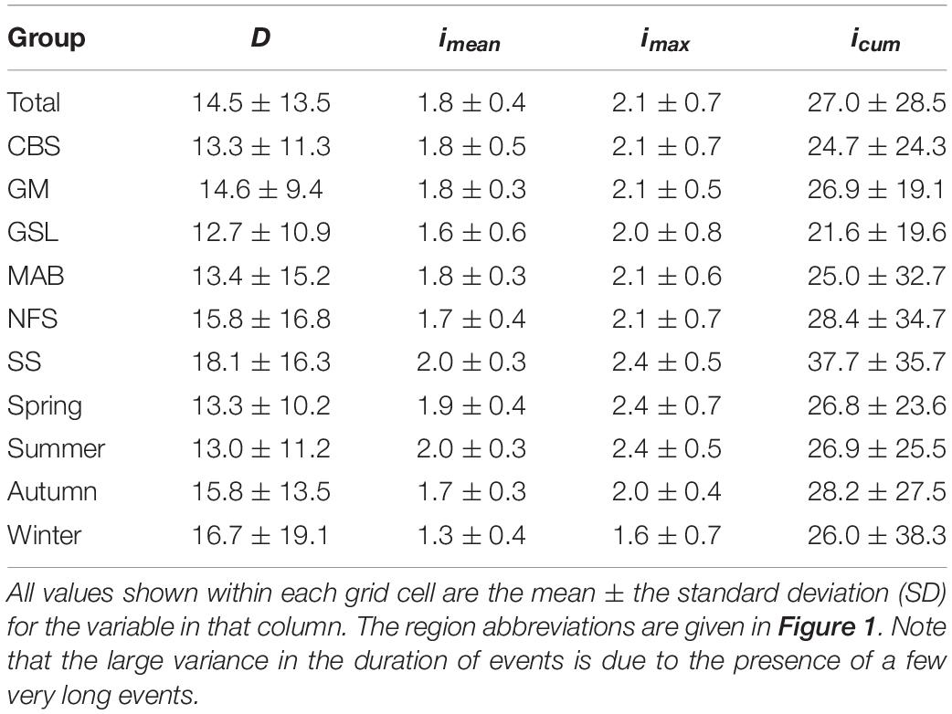
Table 1. The central tendency for the duration (D, days), mean intensity (i_mean; °C), maximum intensity (i_max; °C), and cumulative intensity (i_cum; °C days) for MHWs for the total study area, by region (for all seasons), and by season (for all regions).

Across all regions, there were almost twice as many MHWs detected in Summer (105) as there were in Spring (58) and Winter (58; Figure 1A). MHWs detected in the winter were on average the longest but least intense (Table 1). It must be noted that while the Winter events were the least intense on average, the variance in cumulative intensities was the highest, meaning that there was also a greater probability for large events compared to other seasons. This result is consistent with previous findings that temperature in the MAB during wintertime has the largest interannual variability and is subject to highly variable atmospheric and oceanic forcings (Connolly and Lentz, 2014; Chen et al., 2016). The Summer MHWs were the shortest but most intense. The Spring events were similar to the Summer events, and the Autumn events a mix between Spring and Winter.

Of the 291 MHWs detected across the regions in this study, 251 had an onset phase at least 3 days in length, and 241 MHWs had a decline phase of at least 3 days. This threshold is necessary to allow for the calculation of the following measures of agreement.

Measures of Agreement

Magnitude

Analysis of the dominant drivers during the onset and decline of MHWs reveals remarkable contrast. It was found that more of the change in SSTa during the onset of MHWs could be attributed to T_Qnet than for the decline (Figure 2). As SSTa became larger during the onset of MHWs, T_Qnet often matched or exceeded the magnitude of increase in SSTa, suggesting that the anomalous air–sea fluxes drove the onset. This scenario is less common during declines (Figure 2A). The median proportion of change in SSTa during the onset of MHWs attributable to T_Qnet was 0.46, and for the decline of events this was −0.04 (Figure 2B). This means that overall air–sea heat flux plays an important role for the intensification of MHWs, but does not consistently contribute to the decline of the temperature anomalies. In just under half of the declines of the recorded MHWs (110 out of 243), anomalous air–sea flux continues to be positive (i.e., ΔT_Qnet > 0) while the actual temperature is decreasing (ΔSSTa < 0; Figure 2B). In such cases, oceanic processes (e.g., horizontal heat divergence) are responsible for the decline of the temperature anomalies. This is much less common during the onset of events where the vast majority have at least some increase in temperature attributable to positive changes in T_Qnet (207 out of 251; Figure 2B).

FIGURE 2

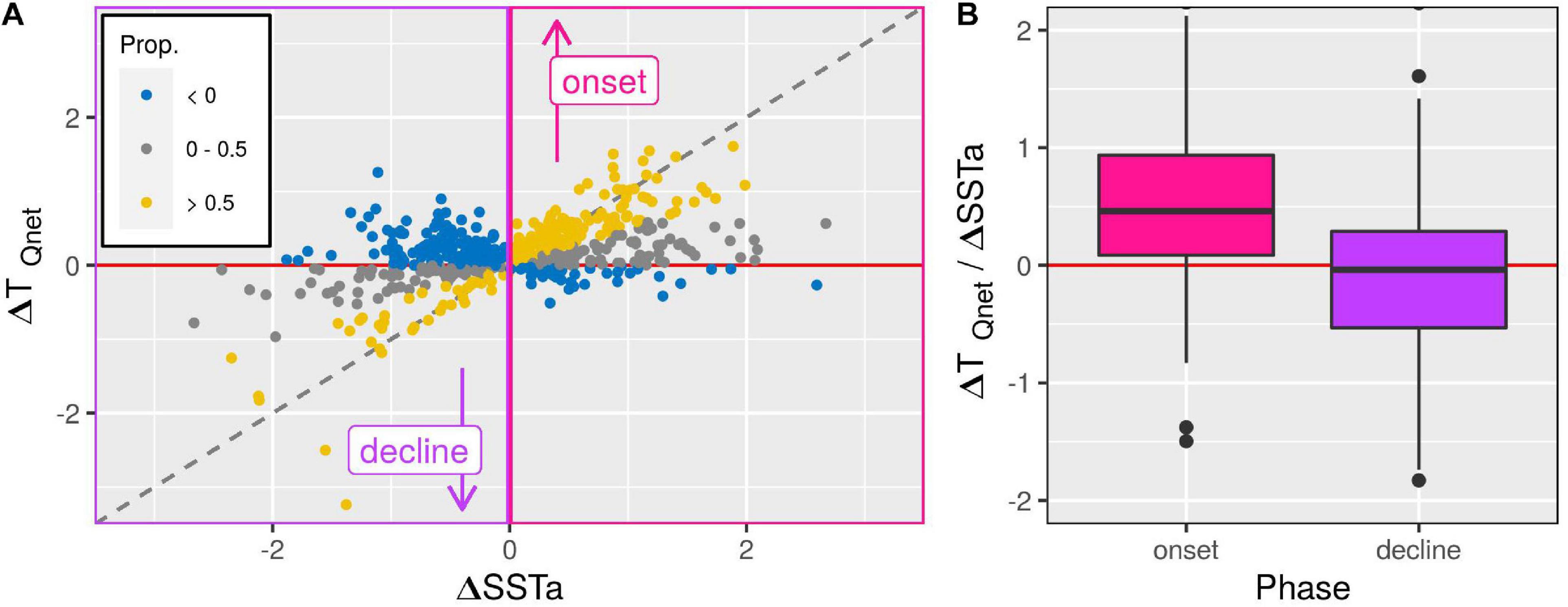
Figure 2. Plots showing the ranges in the contributions of T_Qnet to SSTa during the onset and decline of marine heatwaves (MHWs). (A) Scatterplot showing how the magnitudes of change in SSTa during the onset (ΔSSTa > 0, pink box) and decline (ΔSSTa < 0, purple box) of MHWs matched to T_Qnet. The yellow points show when more than half (0.5) of the proportion of the change in SSTa can be attributed to T_Qnet. Gray points show a positive but not majority input from T_Qnet (0 – 0.5). Blue points show when T_Qnet contributed heat to SSTa contrary to the tendency of the anomaly (i.e., negative heat flux during the onset of a MHW, and positive during the decline). Points falling on the gray dashed line show a one-to-one relationship between SSTa and T_Qnet, while points on the red line show no relationship. (B) Boxplots showing the proportions of change between SSTa and T_Qnet during the onset and decline of all MHWs. The middle black line shows the median proportion of change, and the tops and bottoms of the boxes show the interquartile range (25th–75th percentiles). The whiskers show all MHWs that fall within 1.5 times the interquartile range. Any outliers (black dots) outside of ±2 have been excluded from the plot. The horizontal red line denotes 0, where no contribution to SSTa is being made by T_Qnet. Note that any values below 0 for both onset and decline show that T_Qnet was hindering the onset or decline of the MHW.

Overall, 49% (122 out of 251) of the past MHWs on the Northwest Atlantic shelf had T_Qnet contribute more than half of the increase in SSTa during their onset, but only 17% (42 out of 243) of MHWs had more than half of their declines in SSTa contributed to by T_Qnet (Table 2). Again, this means that air–sea heat flux is much more important for driving MHWs than it is for their decay.

TABLE 2

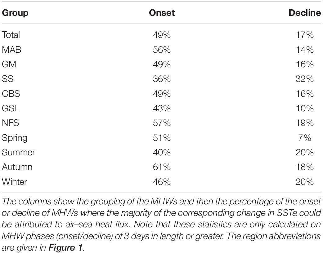
Table 2. The percent of MHWs driven by T_Qnet for the total study area, per region, and per season.

The partition of the primary drivers of MHW during onset vs. decline was similar throughout all of the regions (±9%) with the exception of the Scotian Shelf. The region with the highest percent of MHWs with an onset attributable to T_Qnet was the Newfoundland Shelf (57%), and the lowest was the Scotian Shelf (36%). The region with the greatest percent of MHWs whose decline was attributed to air–sea heat flux was the Scotian Shelf (32%), and the lowest was the Gulf of St. Lawrence (10%).

For seasons, the range of MHW onsets and declines attributable to T_Qnet was greater than for the regions (±12%). The season with the highest percent of MHWs attributable to T_Qnet was Autumn (61%), and the lowest was Summer (40%). The season with the highest percent of MHWs declining due to T_Qnet was a tie between Summer and Winter (20%), the season with the lowest was Spring (7%).

Knowing when the onset or decline of MHWs may be attributed primarily to air–sea heat flux provides us with the broad overview necessary to conclude the importance of this process, but we would also like to know the relative importance of the turbulent and radiative flux terms within T_Qnet during the evolution of SSTa for each event. In the following sub-section we examine the RMSE of T_Qx and SSTa during the onset and decline of MHWs for which T_Qnet was determined to be the primary driver.

Root Mean Square Error (RMSE)

For all seasons the median RMSE for each T_Qx variable during the onset of MHWs is lower than for the decline, with the exception of T_Qlw in Spring (Figure 3A). This is generally true for the regions as well, except for the Gulf of Maine (GM) and the Newfoundland Shelf (NFS) where the RMSE for declines are lower than for onsets (Figure 3B). This means that the T_Qx variables tend to relate more closely during the intensification of a temperature anomaly and less so during their decay. Note that we are only looking at MHWs that are primarily driven by T_Qnet during onset and/or decline, yet there is a closer agreement in the daily development of SSTa during the onset of events. This means that not only are a much higher percentage of the onset of MHWs driven by T_Qnet (see section “Magnitude” and Table 2), the higher frequency variability of the SSTa from start to peak is also better described by the air–sea heat flux terms. This is further support for our finding that air–sea fluxes are more responsible for the onset of MHWs than for their decline, which is likely influenced by ocean advection or mixing.

FIGURE 3

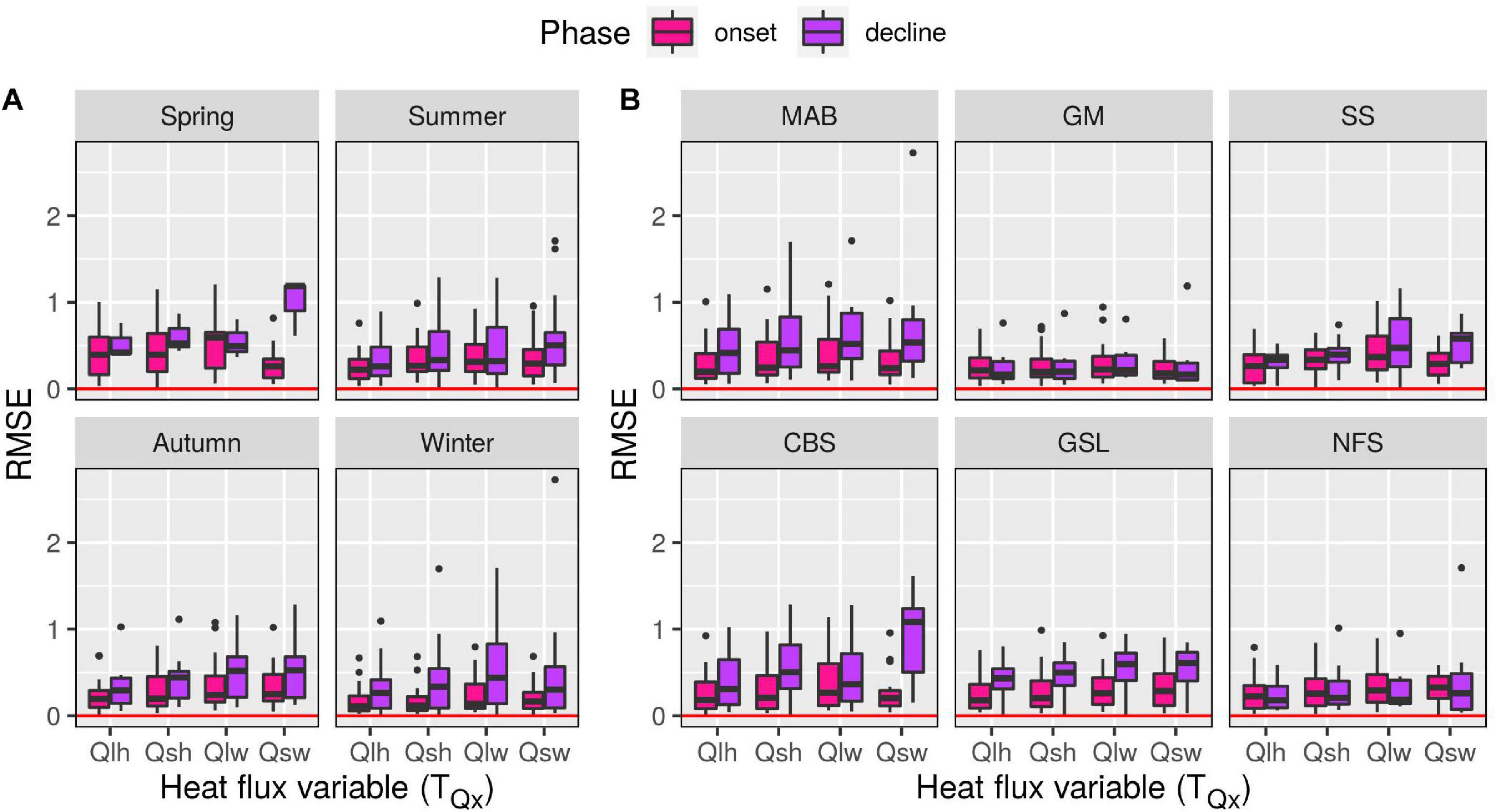
Figure 3. Boxplots showing the range of RMSE values for the T_Qx variables grouped by (A) season and (B) region. The horizontal red line shows a value of 0, which would mean that the daily changes of SSTa and T_Qx are the same. Note that lower RMSE values are better, so the closer to the horizontal red lines the boxplots are, the better that T_Qx variable explains daily changes in SSTa.

The range of RMSE values per season are lowest for onset during Winter, then Autumn, then Summer (Figure 3A). For the decline phase this is reversed, with the lowest values on average found in Summer, then Autumn, then Winter. The RMSE values during spring for both onset and decline are much higher than for the other seasons. This implies that the formation of warm temperature anomalies during the colder months is much more reliant on anomalous T_Qx and that the daily developments in air–sea heat flux more closely match to the daily changes in SSTa. For Spring, however, this is not the case. Even though these RMSE values are limited to only MHWs that were shown to be driven primarily by T_Qnet, the RMSE values for the decline of Spring events are notably larger. This implies higher variability in either SSTa or T_Qx or both. There are also large differences in the RMSE values for the onset and decline of events in the different regions (Figure 3B). Most notable are the very large RMSE values for the decline phase of events in the MAB and Cabot Straight (CBS), where both regions are subject to large advective heat fluxes due to a combination of strong horizontal temperature gradient and proximity to notable ocean currents, i.e., Gulf Stream and coupled Labrador current and St. Lawrence runoff.

For the MHWs driven primarily by T_Qnet, T_Qlh most frequently had the lowest RMSE, and T_Qsw the second lowest (Table 3, rows 1–2). T_Qlw least frequently had the lowest RMSE during the onset of events across all regions and seasons, and for the decline of events it was T_Qsh. This means that for the MHWs driven primary by heat flux anomalies (determined in section “Magnitude”), latent heat flux anomaly most frequently stand out as the major process modulating the SSTa during both onset and decline. In contrast, sensible heat flux and long-wave radiation have less effect in the fluctuation of SSTa during MHWs. This general pattern of lowest and highest RMSE variables applies well across the regions and seasons as well. The warmer seasons more closely follow the overall pattern above that the two variables with the lowest RMSE during onset were T_Qlh and T_Qsw. The decline of events in the warmer seasons were also generally best matched to T_Qlh, but the second best match for both seasons was T_Qlw. Note, however, that there were only three MHWs in Spring whose declines were driven primarily by air–sea heat flux anomalies. The colder seasons of Autumn and Winter differed more in their drivers of onset and decline. The variable with the lowest RMSE during the onset and decline of Autumn events was T_Qlh, with the second lowest RMSE for onset being T_Qsh. Only one MHW in Autumn didn’t have T_Qlh as the most relevant variable during decline. The variables with the lowest RMSE for the onset of Winter MHWs were T_Qsh and T_Qsw, with T_Qlh and T_Qsw tied for having the lowest RMSE during decline. This shows that, unlike the broad similarity in forcing mechanisms across regions, there is a notable seasonal variation in dominant air–sea flux terms, with a more consistent importance of T_Qsh for onsets and declines in the colder months.

TABLE 3

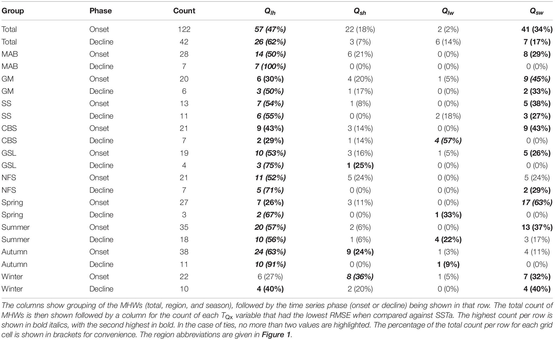
Table 3. The count of which T_Qx variables had the lowest RMSE with SSTa for each MHW, by total, region, and season; split by onset and decline phases.

Correlation

The oceanic and atmospheric states that lead to favorable conditions for surface warming due to air–sea heat flux can be varied. Of the many ocean-atmosphere variables tested as potential drivers for the onset and decline of MHWs, several stood out. The three atmospheric variables that most strongly correlated to SSTa were: T_air (positive), P-E_cum (negative), and MSLP_cum (positive + negative). W_10cum is also worth mentioning for the strong negative relationship it had during the onset of MHWs. The top three oceanic variables were: MLD_cum (negative), SSS (negative), and T_b (positive). This was determined by examining the mean correlation values for each variable, and how non-normal their distributions were. If there were little meaningful relationship between a variable and SSTa we would expect the distribution of the resultant r_x values to look like a normal distribution. For these top variables that is not the case (Figure 4).

FIGURE 4

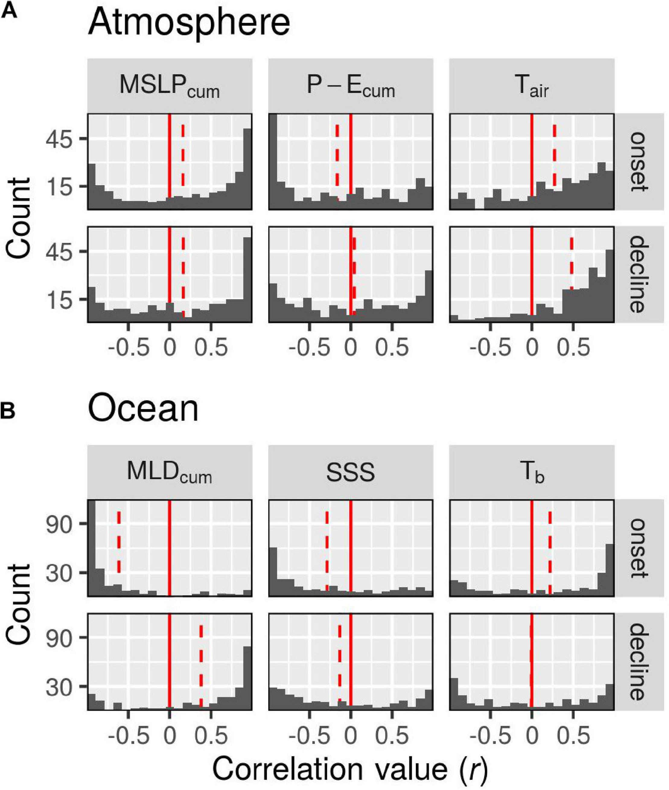
Figure 4. Histograms of correlation values (r) between SSTa and several important candidate forcing variables, shown separately for the onset and decline of marine heatwaves (MHWs). The solid vertical red line on the x-axis shows r = 0, meaning no correlation. The dashed vertical red line shows the mean value in the histogram. Panel (A) contains the results for the top three atmospheric variables, and (B) contains the results for the top three oceanic variables. Note the difference in the y-axes. The variable abbreviations may be found in Sections “Data” and “Agreement Metrics.”

Of the atmospheric variables, T_air had on average the strongest (positive) correlation during the onset of MHWs (Figure 4A). Out of both the atmospheric and oceanic variables, MLD_cum had on average the strongest (negative) correlation with the onset of MHWs (Figure 4B). This implies that of all of the non-heat flux variables that one could use to predict MHW onset, MLD_cum may be the most important. For the decline of MHWs, the two most strongly correlated variables are again T_air and MLD_cum. One important result to note here, however, is that the negative relationship MLD_cum has with the onset of MHWs means that a shoaling of the mixed layer is likely driving the MHW, but the positive relationship MLD_cum has with the decline of MHWs means that the mixed layer is continuing to remain shallow throughout the decay of these events. This is yet another point of support for the conclusion that oceanic processes are more responsible for the decline of MHWs.

There were differences in the strength of these correlations between the different regions and seasons, with the differences being more pronounced across seasons. Generally speaking, MHWs that occurred in Spring and Summer showed similar means and interquartile ranges to each other for the correlations with the top air/sea variables (Figure 5). Autumn and Winter MHWs tended to have similar interquartile ranges of correlations, too, but Autumn events could also occasionally be similar to Spring/Summer events (Figure 5). One important difference is the role of MLD_cum in the onset and decline of Winter MHWs. This variable is consistently strongly correlated to MHW onset and decline, except in Winter when the distribution is much more normal (centered around 0), meaning there is no clear relationship (Figure 5B; MLD_cum). This is because the water column is generally well mixed in most regions during winter and the mixed layer depth is large with little variation. Similarly, many Autumn MHWs also had little to no correlation with MLD_cum during their decline.

FIGURE 5

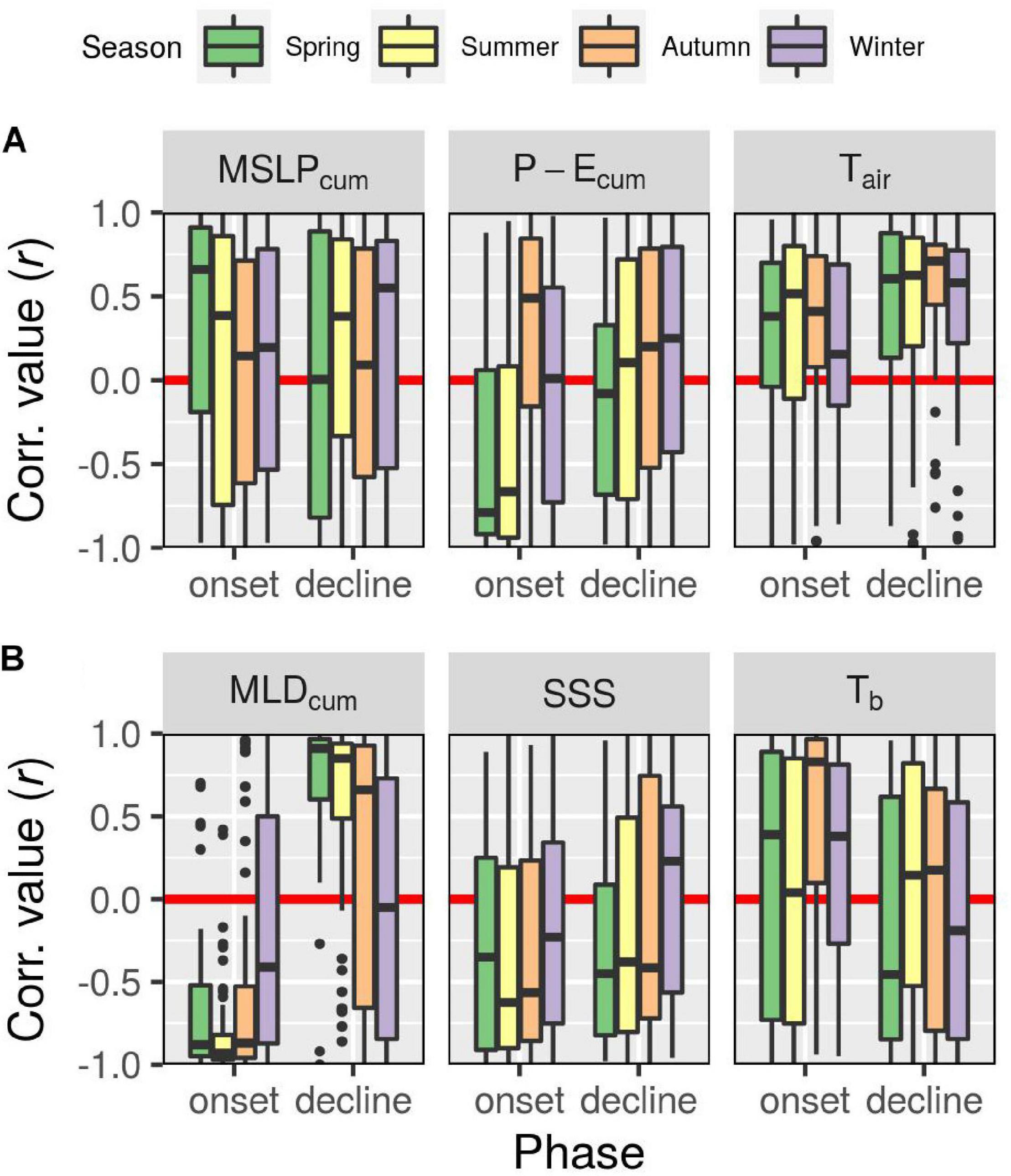
Figure 5. Boxplots showing the range of correlation values (r) between SSTa and the top three atmospheric and oceanic variables, grouped by season and marine heatwave (MHW) phase. The horizontal red line shows r = 0, where no correlation is found. The variables are divided into panels (A) atmospheric and (B) oceanic. The center black line in the boxplots is the median value, and the tops and bottoms are the interquartile range (25th – 75th percentiles). The whiskers show all other values falling within 1.5 this interquartile distance, and the black dots are outliers. The further from the red line the center of the boxplots are, the less normal, and therefore more meaningful the relationship with that variable and MHW onset or decline is. The variable abbreviations may be found in Sections “Data” and “Agreement Metrics.”

Self-Organizing Map (SOM)

The 291 MHWs across all regions were clustered into a 12 node (4 × 3) SOM, with each node displaying different ocean and atmospheric patterns associated with MHWs. Even though the region and season of occurrence of each MHW was not provided to the SOM, it still clustered MHWs in noticeable patterns expressed in these attributes. Of the many variables that were fed to the SOM, it was the atmospheric variables that came through with the clearest patterns.

Before addressing the output of the SOM it is important to note the differences in the MHWs clustered into each node. The central two nodes (F, G) had the highest counts of all clustered MHWs and these events also tended to have the longest lasting, most intense events from the study (Table 4). The MHWs from node J were also amongst the longest lasting and most intense. The shortest, least intense MHWs were found in three of the four corner nodes: D, I, and L.

TABLE 4

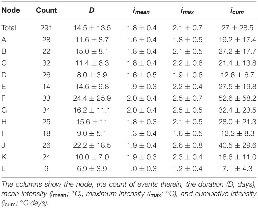
Table 4. The mean ± standard deviation of the MHW metrics for the total collection of events as well as each node from the SOM analysis.

The methodology in this study was intentionally structured with MHWs occurring simultaneously across regions so that we could investigate the similarity of their synoptic scale forcing with the SOM. Of the 291 MHWs in this study, there were 321 pairs of events that overlapped by at least 1 day or more. Note that one MHW could overlap with multiple other events. Of these 321 overlapping pairs, 190 of them were clustered into the same Nodes. Of the 131 pairs that were not clustered together, 74 of them had at least one short (<10 days) event that didn’t overlap much with its paired MHW. Indeed, the median proportion of overlapping days for events not clustered together was 0.21, and 0.47 for clustered events. This shows us that when synoptic scale patterns are causing multiple MHWs simultaneously across regions the SOM clusters these together accordingly, with the exception of when one of the events is very short, or the events that don’t overlap by many days. For the shorter events this is likely because the cause of these events is a more transient driver that isn’t resolved as clearly in the mean synoptic state for the longer event. When the events don’t overlap by many days they will generally be related to different drivers that are emerging in close temporal proximity, but are not the same phenomenon and so are not clustered together in the SOM.

In the following sub-sections we will focus on the regional/seasonal and atmospheric patterns from the SOM as these provide the most clear and meaningful results. The figures showing the patterns for the SST + surface currents (Supplementary Figure 1) and Q_net + MSLP (Supplementary Figure 2) can be found in the supplementary, as well as a figure showing the date of occurrence, duration, and maximum intensity of the MHWs clustered into each node (Supplementary Figure 3).

Regions and Seasons

The central nodes tended to have more MHWs clustered into them (n ≥ 33) than the outer nodes (n = 9–32; Figure 6). The nodes in the top right corner (Figure 6; C, D, H) are filled mostly with events centered around the MAB and only a couple of events on the NFS. The top left corner nodes (A, B, E) have mostly NFS and CBS events. The distribution of MHWs is less focused within the same single region throughout the center two columns of nodes, though some nodes do show a tendency toward regionality. There is no apparent regional pattern as one moves from the top to the bottom.

FIGURE 6

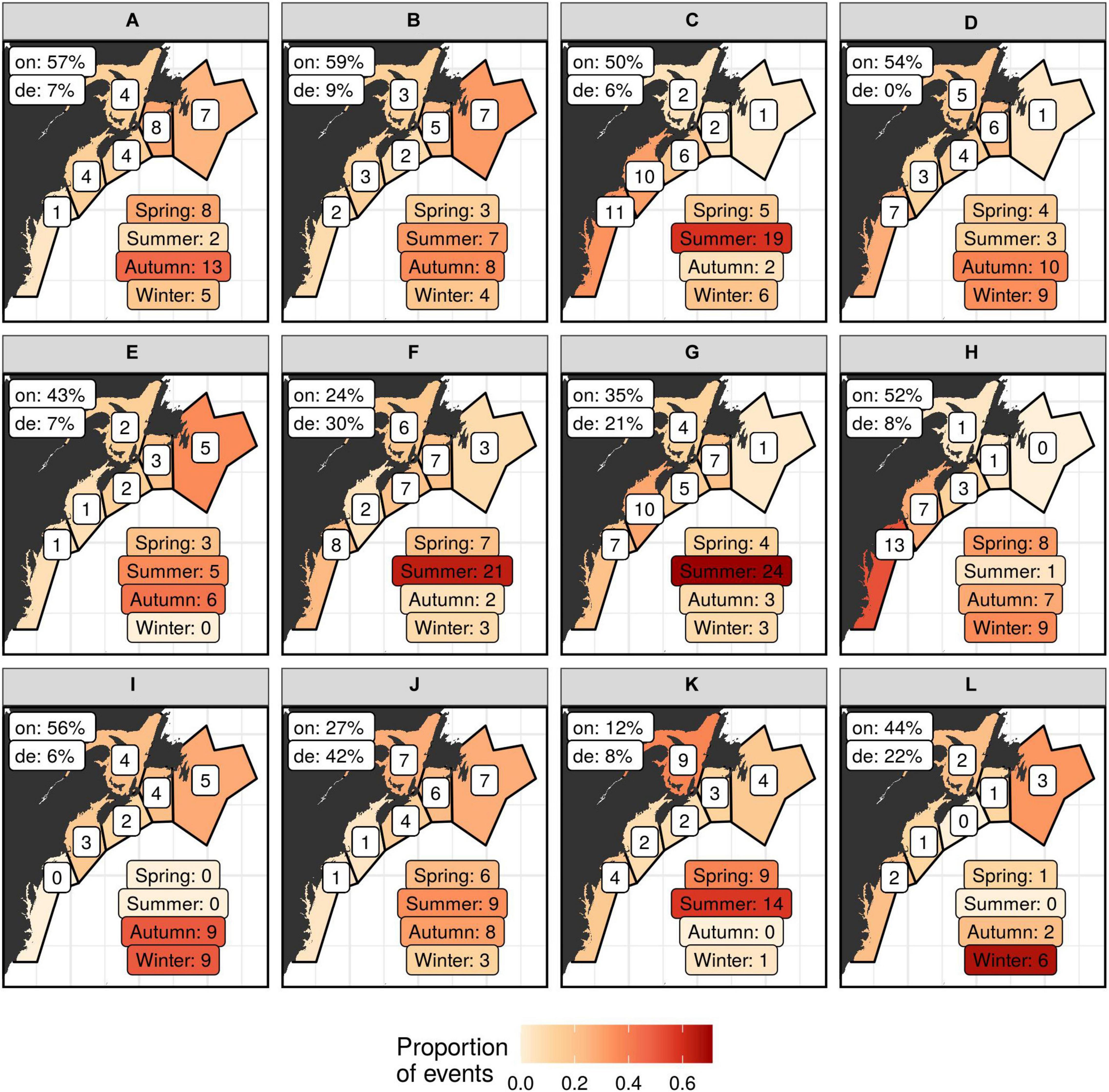
Figure 6. The count of marine heatwave (MHW) occurrence across seasons and regions clustered into the 12 SOM nodes (A–L). The count of MHWs in each region are shown with white labels over the given region. The count of MHWs per season are shown in labels in the bottom right of each panel. The percentage of MHWs whose onset (on) or decline (de) was contributed to primarily by T_Qnet are shown in the top left of each panel. Note that on average 49% of the onset of MHWs are driven by T_Qnet and 17% of declines.

For seasonal patterns, we see that the MHWs occurring in the middle two nodes (F, G) and the center-right column (C, G, K) are primarily summer events (Figure 6). The nodes in the left column (A, E, I) are predominantly Autumn events with high proportions in the neighboring seasons. The nodes in the right column (D, H, L) are predominantly Autumn and Winter events, with some occurring in Spring as well. The bottom right node (L) has a very high proportion of events in Winter and none in Summer.

The top row (A, B, C, D) and two side nodes (H, I) show MHWs with high proportions of onsets driven by T_Qnet, and low proportions of declines. The bottom four central nodes (F, G, J, K) show MHWs where the onsets were driven similarly or less than the declines by T_Qnet.

Atmospheric Variables

For air temperature anomalies we see that the air overlying the ocean in the east of the study region gets warmer as we move left and down through the nodes (Figure 7). The air over the continent becomes warmer as we move to the top right corner. The air temperatures for the middle top four nodes (B, C, F, G) are moderately warm over nearly the full study area. The air over the Atlantic Ocean tends to become warmer as we move up the nodes. The bottom row shows stronger meridional (North–South) temperature gradients whereas the top row tends toward stronger zonal (East–West) temperature gradients. The nodes in the bottom right (G, H, K, L) generally show northerly air flow whereas the top row and left column are mostly southerly air flow. If we compare these regions of high air temperature anomalies (Figure 7) to the regions of highest MHW occurrence (Figure 6), we see that there is a strong relationship between the two. This supports the earlier observation that the best atmospheric predictor of MHWs is T_air (Figure 4). This is also why we see either strong negative or positive correlations for MSLP (Figure 4), because both low-pressure and high-pressure systems may be present during MHWs.

FIGURE 7

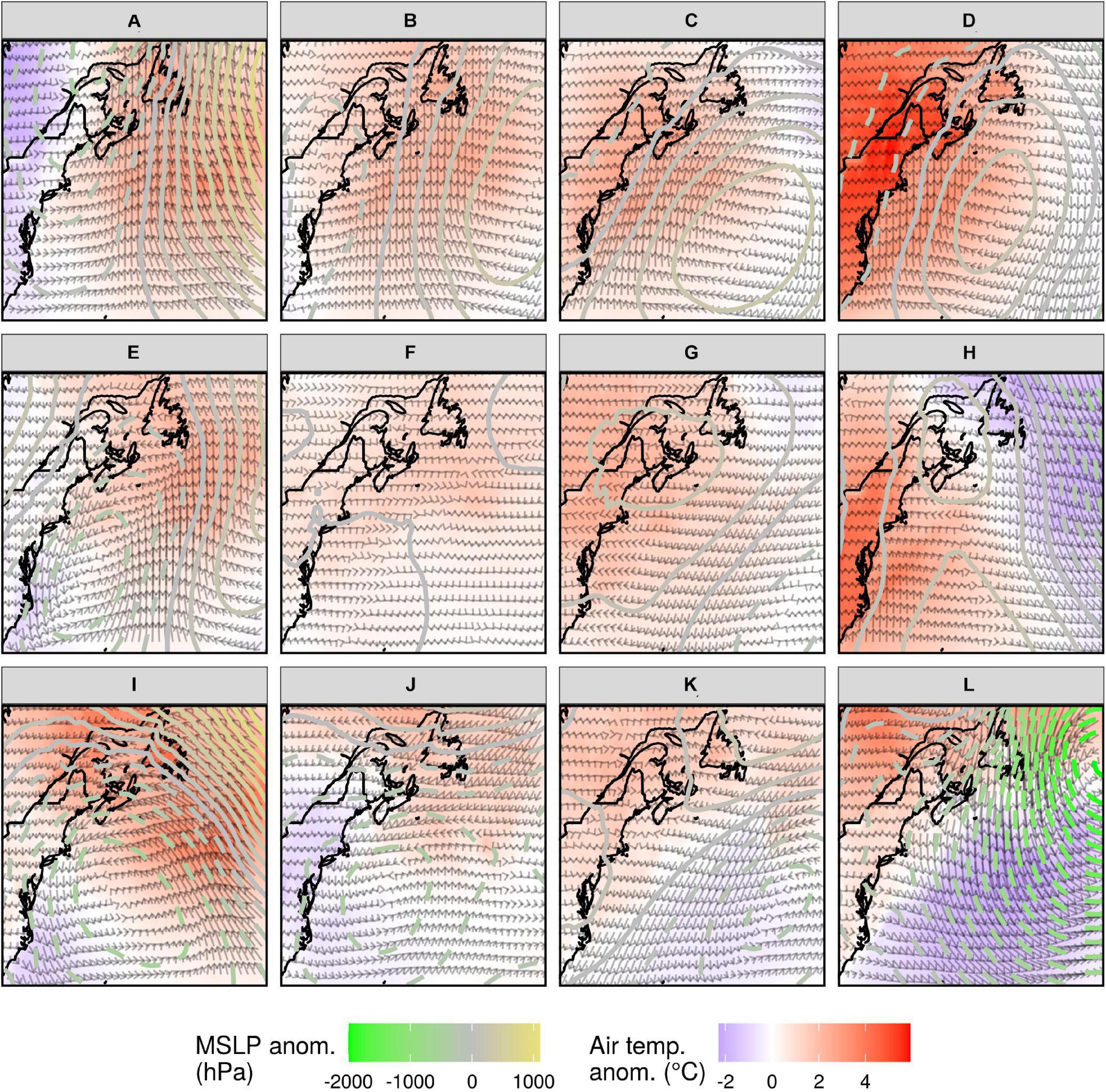
Figure 7. The average synoptic states for anomalous air temperature, wind speed/direction (vectors), and MSLP (mean sea-level pressure) for each node in the SOM results (A–L). Solid contours show positive MSLP anomaly and dashed contours show negative MSLP anomaly. The background colors of red to blue indicate air temperature anomaly. Note that MSLP was not one of the variables fed to the SOM, but is shown here to better outline the patterns in the wind and air temperatures.

In most of the top row and right column nodes (Figures 7B–D,H) we see high-pressure blocking anticyclonic wind anomalies around thermal dipoles of varying magnitude with the northward moving air being anomalously warm; the warmer (colder) the anomaly the faster north (south) the anomalous wind movement is. We tend to see the opposite (low pressure systems) in the left column and bottom row (A, E, I, J, K, L). The air temperature anomalies for these low pressure cyclones tend to be less than for the high pressure anticyclones, but the pressure gradients and wind speeds are much stronger. The center nodes (F, G) are relatively quiescent states, i.e., the “dog days of summer.” Nodes I and L very prominently display similar Autumn/Winter low pressure systems (Figures 6, 7). Node I shows this system linked with MHWs as it nears the Scotian Shelf, and node L shows the system not linked with MHWs until it has nearly passed from the study area. While it may appear that the Node I pattern should precede the Node L pattern in time, the average difference in days between events in these nodes is nearly 2 years. There is only one event in Node L that occurs within 2 weeks of an event in Node I.

A common pattern that emerges between atmospheric states and the onset/decline of MHWs driven by T_Qnet is that any system that bring warm air up from the South onto the coast are more likely to drive the onset of MHWs due to heat flux than any other pattern. This same pattern is likewise the least likely to have heat flux driving the decline of the events that they have created. In these results this is predominantly caused by high pressure blocking systems accompanied by anti-cyclonic wind anomalies, but some low-pressure systems also cause southerly winds. Zonal systems that lead to relatively quiescent states have a much lower likelihood of being associated with the driving of the onset of MHWs by T_Qnet, but a much higher likelihood that the decline of events will be due to T_Qnet. The MHWs in these nodes are also, on average, the longest and most intense.

Discussion

In this paper we investigated the relationship between air–sea heat flux and the onset and/or decline of MHWs. This was done through a four step methodology: (1) finding the proportion of change in SSTa attributable to T_Qnet, (2) finding the RMSE of SSTa and T_Qx for MHWs whose onset and/or decline was driven predominantly by T_Qnet, (3) correlations between SSTa and ocean-atmosphere state variables, and (4) a SOM analysis of the mean synoptic states during MHWs. It was found that air–sea heat flux is responsible for the onset of roughly half of the MHWs in the chosen study area, but less than a fifth of the declines. It was also found that T_Qlh and T_Qsw matched much more closely to daily changes in SSTa and that these differences were not the same across regions/seasons. Of the many ocean-atmosphere state variables investigated, T_air and MLD_cum were found to have the strongest relationships with MHW onsets and declines; with MLD_cum decreasing during MHW onset and T_air decreasing during MHW decline. Lastly, the SOM analysis revealed that both low-pressure systems and high-pressure blocking cells could be present during the occurrence of MHWs.

Measures of Agreement

The relationship between T_Qnet and SSTa has lead us to infer that MHW onset in the NW Atlantic is predominantly forced by air–sea heat flux, while MHW decay is likely due to ocean advective or mixing processes not captured in our analysis. Not only is air–sea heat flux driving the onset of nearly half of the MHWs in the NW Atlantic and less than one fifth of the declines, when MHW decline may be attributed to air–sea heat flux, the fit of the T_Qx variables to declining SSTa is worse. This is more support for our inference that the decline of MHWs is more often related to oceanic processes, e.g., advective flux, which is not explicitly captured in our methodology. The variable with the best correlation with SSTa during the decline of a MHW is T_air. This alone is likely not what is driving the SSTa anomaly, but is rather a secondary variable being controlled by the same advective/mixing process responsible for the decline in the SSTa, or is itself being driven by the changes in SST.

It was also seen that MLD_cum tended to have a strong positive correlation with SSTa during the decline of the events, implying a continued shoaling of mixed layer during the decline phase (a negative correlation would mean that the MLD is deepening as the temperature anomaly went back down to zero). This means that most MHWs begin when the MLD is shoaling, or has already shoaled, but then the MLD does not begin to deepen again at the decline of the event. Advective or mixing processes must thus be responsible for the decline of the temperature anomaly. It may also be that the T_Qx variables are not found to relate closely to SSTa at the decline of events specifically because of the lack of MLD agreement during the decline phase. This continued shoaling of the MLD during the end of MHWs implies that a shoaled MLD may be a more long-lasting features than the MHWs, and may actually be the driving force behind the occurrence of two or more short events in rapid succession. This observation was tested, but it was found that short events (<10 days duration) occurring within 2 weeks or less of each other were almost always accompanied by an anomalously deep MLD, not shallow.

Self-Organizing Map (SOM)

We saw from the SOM that there were three primary types of patterns. (1) Low pressure cyclonic systems that occurred mostly in Autumn and Winter. (2) High pressure blocking systems with anticyclonic wind anomalies that occurred mostly in the Spring and Summer; and (3) high pressure blocking cells that would sit over the study area for long periods of time almost exclusively in Summer. A brief synopsis of the dominant patterns of each node has been tabularized for convenience (Table 5).

TABLE 5

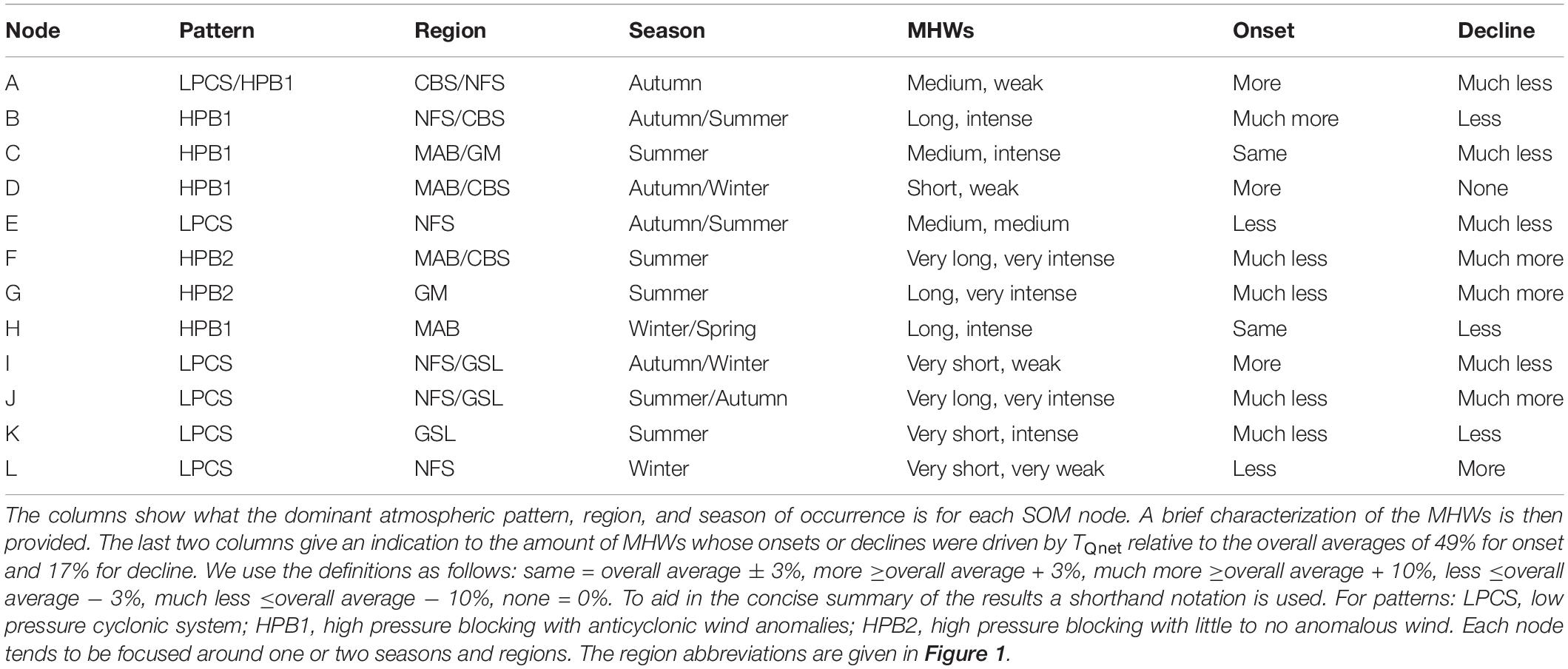
Table 5. A typology of marine heatwaves (MHWs) as categorized by the SOM.

It was also noted that when the onset of a MHWs was driven by T_Qnet, it was much more likely that the predominant atmospheric pattern present was bringing warm southerly wind against the coast. This could be due to low pressure systems, but was more often due to high pressure blocking. This same pattern was also very infrequently related to MHWs whose decline was driven primarily by T_Qnet. Note also that the quiescent atmospheric states associated with long lasting and intense MHWs were also much more likely to occur during MHWs whose declines were driven by T_Qnet. This provides two very strong starting points for future research on the relationships between atmospheric drivers of air–sea heat flux and the formation of MHWs.

Methodology

The novel methodology created for this study has proven effective at quantifying and numerating the processes responsible for the onset and decline of MHWs, but there are some issues that demand further consideration. One such issue is how best to arrive at the definition of a single MHW when multiple smaller events occur within a short period of time. For consistency throughout this study we adhered to the method for MHW detection from Hobday et al. (2016), which states that events are counted as separate once the daily SST value drops below the 90th percentile threshold for more than 2 days. We acknowledge that this definition for gaps between events could be debated further, but here we stick to the definition to be consistent with earlier studies. Large and intense events may occur over broad spatiotemporal scales and may have long-lasting impacts on the background state. As a result, a large and intense event may be detected as multiple MHWs in different regions and/or as multiple MHWs close to each other in time. Even so, the onset and decay of these individual MHWs across space and time may not necessarily be driven by the same processes. In this study we decided to keep the smaller events separate from each other in order to provide the measures of agreement between datasets as rich a diversity of ‘types’ of MHWs as possible. Along this same avenue of thought we opted out of performing any additional smoothing on the SST time series. This could have potentially worked to join short rapidly occurring MHWs together without compromising on the pre-established methodology, but that in turn would have exaggerated the importance of these minor events by combining them into much longer single events. The effect of low-pass smoothing on MHW detection would also make for an interesting future study, though to some extent it is already known that the further smoothing of the seasonal climatology used for MHW detection leads to the detection of more intense events in Summer/Winter and less intense events in Spring/Autumn (Schlegel et al., 2019). Finally, it is known that preconditioning is an important consideration for the study of anomalous temperatures in the NW Atlantic (Chen et al., 2016). This methodology does not account for preconditioning specifically as this falls outside of its scope. Given the known importance of this phenomenon in the area it would be an excellent topic to investigate in more depth in a future study. As we have shown here with a follow up investigation into the potential for a shoaled MLD to function as preconditioning for short rapid MHWs, the relationship of this phenomenon with MHWs is not as clear as would be hypothesized and deserves further study.

A final and interesting consideration that was not accounted for in this methodology was the effect that anthropogenic warming will have on the SOM analysis. Consider that as the world is gradually warming, it becomes relatively easier for an atmospheric or oceanic driver to force a MHW because the SST values needed in order to be above a historic climatology are less than they would be in the cooler past. This means that a more intense synoptic scale pattern would need to be present to drive MHWs in the past than in the future. However, most of the SOM nodes contain MHWs that occur over the whole time range of 1993 – 2018, so any possible warming signal appears not to have had a noticeable impact on the results. It would, however, be an interesting study to look at results from much longer (centennial-scale) time series to see at what point anthropogenic warming has a significant impact on the types of synoptic scale forcing that can be related to the occurrence of MHWs.

Conclusion

In this study we used a suite of agreement metrics to develop an overall understanding of the drivers of the onset and decline of MHWs over the NW Atlantic continental shelf. It was found that nearly half (49%) of the onset of MHWs could be attributed to air–sea heat flux, but less than a fifth (17%) of the decline of MHWs could be attributed to the same process. Of the individual T_Qx variables, T_Qlh and T_Qsw were most frequently the top two relevant drivers of the onset and decline of MHWs across all regions and seasons. T_Qlw was on average the least important (highest RMSE value) for onsets, and T_Qsh for declines across all regions and seasons. Over the entire study domain, T_Qlh and T_Qsw were still the most important drivers for onset in all seasons, but for the colder seasons of Winter and Autumn the onset of events often corresponded better to T_Qsh. Anomalous air–sea heat fluxes are responsible for the onset and decline of more MHWs during the cold seasons (on average), and anomalous advection may be more responsible for MHWs during the warm seasons. This is presumably associated with the seasonal variability of advective fluxes, and is consistent with the results in Chen and Kwon (2018).

Air–sea heat flux alone may not be the only potential driver, or indicator of the development of MHWs. In order to have a better understanding of the driving processes, we further evaluated the correlations between SSTa and a suite of atmospheric and oceanic state variables. It was found that the top state variables to correlate with SSTa were T_air and MLD_cum. This shows that not only does the heat flux itself (i.e., Q_x) play a role, but importantly MLD shoaling is critical for the onset of most events. In comparison, the decline of MHWs was strongly positively correlated to T_air. It must be noted, however, that the decline of most MHWs are not explainable via air–sea heat flux, which implies that the strong relationship that T_air has with SSTa during the decline of MHWs should not be over-interpreted. It appears that persistent atmospheric forcing is necessary to maintain MHWs, so that when this forcing dissipates other processes (presumably oceanic processes) can take over and dissipate the accumulated heat in the mixed-layer associated with the MHW. The answer to what drives the decline of MHWs lies in a wider, more comprehensive future analysis that includes ocean advection and mixing.

Lastly, in order to identify common synoptic scale patterns during MHWs a SOM analysis was used. From this we determined that there were three primary atmospheric patterns during MHWs. The first was a high pressure blocking cell present over the region accompanied by anticyclonic wind anomalies, usually in the warmer months, causing anomalously high levels of heat flux through the ocean surface. These patterns were most (least) often associated with MHW onsets (declines) driven by T_Qnet. The second pattern was a low-pressure cyclonic system present over the region, usually in the colder months, that transported heat into the region from elsewhere and provided strong winds to enhance air–sea heat fluxes. The final pattern was found most often in the warmer months, and was associated with the longest and most intense MHWs. This is the “dog days of summer” type of synoptic pattern in which the wind, air, and MSLP exhibit weakly anomalous behavior, but they persist for much longer than they normally would and create a slow and steady build up of heat in the surface of the ocean. These patterns were most frequently associated with MHW declines driven by T_Qnet.

Data Availability Statement

The datasets generated for this study can be found in online repositories. The names of the repository/repositories and accession number(s) can be found below: https://github.com/robwschlegel/MHWflux.

Author Contributions

RS led the study and prepared the majority of the text, figures, synthesized the comments, and uploaded the manuscript. EO conceptualized the SOM portion of the study. KC conceptualized the magnitude and RMSE portions of the study. EO and KC both provided guidance on the physical oceanographic aspects of the study. RS conceptualized the correlation portion of the study and introduced the idea to split the analyses into onset/decline phases. EO and KC provided several rounds of comments on the manuscript as it was developed. All authors provided responses to reviewers during the editorial process.

Funding

RS was supported by the Ocean Frontier Institute International Postdoctoral Fellowship hosted jointly by Dalhousie University and Woods Hole Oceanographic Institution, through an award from the Canada First Research Excellence Fund. EO was funded through the National Sciences and Engineering Research Council of Canada Discovery Grant RGPIN-2018-05255 and Marine Environmental Observation, Prediction, and Response Network Early Career Faculty Grant 1-02-02-059.1. KC was supported by National Oceanic and Atmospheric Administration Climate Program Office Modeling, Analysis, Predictions, and Projections (MAPP) program under grant NA19OAR4320074 and Climate Variability and Predictability (CVP) program under grant NA20OAR4310398.

Conflict of Interest

The authors declare that the research was conducted in the absence of any commercial or financial relationships that could be construed as a potential conflict of interest.

Acknowledgments

The authors would like to acknowledge the input of the two reviewers whose constructive comments greatly improved the quality of the manuscript. The authors would like to acknowledge Balagopal Pillai and the Department of Mathematics and Statistics, Dalhousie University for hosting and administrating the high-performance computing infrastructure that supported this study. The authors would like to acknowledge NOAA for providing the OISST v2.1 data, which may be downloaded from: https://www.ncei.noaa.gov/data/sea-surface-temperature-optimum-interpolation/v2.1/access/avhrr/; ECMWF for providing ERA5 data, a tutorial for downloading may be found here: https://confluence.ecmwf.int/display/CKB/How+to+download+ERA5; and Copernicus for providing GLORYS data, which may be downloaded from: https://marine.copernicus.eu/. A tutorial for how to download and process these data in R may be found here: https://theoceancode.netlify.app/post/dl_env_data_r/.

Supplementary Material

The Supplementary Material for this article can be found online at: https://www.frontiersin.org/articles/10.3389/fmars.2021.627970/full#supplementary-material

References

Akinduko, A. A., Mirkes, E. M., and Gorban, A. N. (2016). SOM: stochastic initialization versus principal components. Inform. Sci. 364, 213–221. doi: 10.1016/j.ins.2015.10.013

CrossRef Full Text | Google Scholar

Barnes, E. A. (2013). Revisiting the evidence linking Arctic amplification to extreme weather in midlatitudes. Geophys. Res. Lett. 40, 4734–4739. doi: 10.1002/grl.50880

CrossRef Full Text | Google Scholar

Banzon, V., Smith, T. M., Chin, T. M., Liu, C., and Hankins, W. (2016). A long-term record of blended satellite and in situ sea-surface temperature for climate monitoring, modeling and environmental studies. Earth Syst. Sci. Data 8, 165–176. doi: 10.5194/essd-8-165-2016

CrossRef Full Text | Google Scholar

Banzon, V., Smith, T. M., Steele, M., Huang, B., and Zhang, H.-M. (2020). Improved estimation of proxy sea surface temperature in the arctic. J. Atmos. Ocean. Technol. 37, 341–349. doi: 10.1175/JTECH-D-19-0177.1

CrossRef Full Text | Google Scholar

Benthuysen, J., Feng, M., and Zhong, L. (2014). Spatial patterns of warming off Western Australia during the 2011 Ningaloo Niño: quantifying impacts of remote and local forcing. Continent. Shelf Res. 91, 232–246. doi: 10.1016/j.csr.2014.09.014

CrossRef Full Text | Google Scholar

Blackport, R., and Screen, J. A. (2020). Insignificant effect of Arctic amplification on the amplitude of midlatitude atmospheric waves. Sci. Adv. 6:eaay2880. doi: 10.1126/sciadv.aay2880

PubMed Abstract | CrossRef Full Text | Google Scholar

Bond, N. A., Cronin, M. F., Freeland, H., and Mantua, N. (2015). Causes and impacts of the 2014 warm anomaly in the NE Pacific. Geophys. Res. Lett. 42, 3414–3420. doi: 10.1002/2015GL063306

CrossRef Full Text | Google Scholar

Cavazos, T. (2000). Using self-organizing maps to investigate extreme climate events: an application to wintertime precipitation in the Balkans. J. Clim. 13, 1718–1732. doi: 10.1175/1520-0442(2000)013<1718:usomti>2.0.co;2

CrossRef Full Text | Google Scholar

Chen, K., Gawarkiewicz, G., Kwon, Y. O., and Zhang, W. G. (2015). The role of atmospheric forcing versus ocean advection during the extreme warming of the Northeast US continental shelf in 2012. J. Geophys. Res. Oceans 120, 4324–4339. doi: 10.1002/2014JC010547

CrossRef Full Text | Google Scholar

Chen, K., Gawarkiewicz, G., Lentz, S. J., and Bane, J. M. (2014a). Diagnosing the warming of the Northeastern U.S. Coastal Ocean in 2012: a linkage between the atmospheric jet stream variability and ocean response. J. Geophys. Res. Oceans 119, 218–227. doi: 10.1002/2013JC009393

CrossRef Full Text | Google Scholar

Chen, K., He, R., Powell, B. S., Gawarkiewicz, G. G., Moore, A. M., and Arango, H. G. (2014b). Data assimilative modeling investigation of Gulf Stream Warm Core Ring interaction with continental shelf and slope circulation. J. Geophys. Res. Oceans 119, 5968–5991. doi: 10.1002/2014JC009898

CrossRef Full Text | Google Scholar

Chen, K., and Kwon, Y. O. (2018). Does pacific variability influence the northwest atlantic shelf temperature? J. Geophys. Res. Oceans 123, 4110–4131. doi: 10.1029/2017JC013414

CrossRef Full Text | Google Scholar

Chen, K., Kwon, Y. O., and Gawarkiewicz, G. G. (2016). Interannual variability of winter-spring temperature in the Middle Atlantic Bight: relative contributions of atmospheric and oceanic processes. J. Geophys. Res. Oceans 121, 4209–4227. doi: 10.1002/2016JC011646

CrossRef Full Text | Google Scholar

Chen, Z., Kwon, Y. O., Chen, K., Fratantoni, P., Gawarkiewicz, G., and Joyce, T. M. (2020). Long-term SST variability on the northwest atlantic continental shelf and slope. Geophys. Res. Lett. 47:e2019GL085455. doi: 10.1029/2019GL085455

CrossRef Full Text | Google Scholar

Connolly, T. P., and Lentz, S. J. (2014). Interannual variability of wintertime temperature on the inner continental shelf of the Middle Atlantic Bight. J. Geophys. Res. Oceans 119, 6269–6285. doi: 10.1002/2014JC010153

CrossRef Full Text | Google Scholar

Copernicus Climate Change Service [C3S] (2017). ERA5: Fifth Generation of ECMWF Atmospheric Reanalyses of the Global Climate. London: Copernicus Climate Change Service.

Google Scholar

Feng, M., McPhaden, M. J., Xie, S. P., and Hafner, J. (2013). La Niña forces unprecedented Leeuwin Current warming in 2011. Sci. Rep. 3,, 1–9. doi: 10.1038/srep01277

PubMed Abstract | CrossRef Full Text | Google Scholar

Forsyth, J. S. T., Andres, M., and Gawarkiewicz, G. G. (2015). Recent accelerated warming of the continental shelf off New Jersey: observations from the CMV Oleander expendable bathythermograph line. J. Geophys. Res. Oceans 120, 2370–2384. doi: 10.1002/2014JC010516

CrossRef Full Text | Google Scholar

Francis, J. A., and Vavrus, S. J. (2012). Evidence linking Arctic amplification to extreme weather in mid-latitudes. Geophys. Res. Lett. 39. doi: 10.1029/2012GL051000

CrossRef Full Text | Google Scholar

Francis, J. A., and Vavrus, S. J. (2015). Evidence for a wavier jet stream in response to rapid Arctic warming. Environ. Res. Lett. 10:014005. doi: 10.1088/1748-9326/10/1/014005

CrossRef Full Text | Google Scholar

Frölicher, T. L., Fischer, E. M., and Gruber, N. (2018). Marine heatwaves under global warming. Nature 560, 360–364. doi: 10.1038/s41586-018-0383-9

PubMed Abstract | CrossRef Full Text | Google Scholar

Garfield, N. III, and Evans, D. L. (1987). Shelf water entrainment by Gulf Stream warm-core rings. J. Geophys. Res. Oceans 92, 13003–13012. doi: 10.1029/JC092iC12p13003

CrossRef Full Text | Google Scholar

Gawarkiewicz, G. G., Todd, R. E., Plueddemann, A. J., Andres, M., and Manning, J. P. (2012). Direct interaction between the Gulf Stream and the shelfbreak south of New England. Sci. Rep. 2:553. doi: 10.1038/srep00553

PubMed Abstract | CrossRef Full Text | Google Scholar

Gibson, P. B., Perkins-Kirkpatrick, S. E., Uotila, P., Pepler, A. S., and Alexander, L. V. (2017). On the use of self-organizing maps for studying climate extremes. J. Geophys. Res. Atmos. 122, 3891–3903. doi: 10.1002/2016JD026256

CrossRef Full Text | Google Scholar

Greenan, B. J. W., Shackell, N., Ferguson, K., Greyson, P., Cogswell, A., Brickman, D., et al. (2019). Climate change vulnerability of American lobster fishing communities in Atlantic Canada. Front. Mar. Sci. 6:579. doi: 10.3389/fmars.2019.00579

CrossRef Full Text | Google Scholar

Hewitson, B. C., and Crane, R. G. (2002). Self-organizing maps: applications to synoptic climatology. Clim. Res. 22, 13–26. doi: 10.3354/cr022013

CrossRef Full Text | Google Scholar

Hobday, A. J., Alexander, L. V., Perkins, S. E., Smale, D. A., Straub, S. C., Oliver, E. C., et al. (2016). A hierarchical approach to defining marine heatwaves. Prog. Oceanogr. 141, 227–238. doi: 10.1016/j.pocean.2015.12.014

CrossRef Full Text | Google Scholar

Holbrook, N. J., Scannell, H. A., Gupta, A. S., Benthuysen, J. A., Feng, M., Oliver, E. C., et al. (2019). A global assessment of marine heatwaves and their drivers. Nat. Commun. 10, 1–13. doi: 10.1038/s41467-019-10206-z

PubMed Abstract | CrossRef Full Text | Google Scholar

Johnson, N. C. (2013). How many ENSO flavors can we distinguish? J. Clim. 26, 4816–4827. doi: 10.1175/JCLI-D-12-00649.1

CrossRef Full Text | Google Scholar

Joyce, T. M., Bishop, J. K., and Brown, O. B. (1992). Observations of offshore shelf-water transport induced by a warm-core ring. Deep Sea Res. A Oceanogr. Res. Pap. 39, S97–S113. doi: 10.1016/S0198-0149(11)80007-5

CrossRef Full Text | Google Scholar

Kavanaugh, M. T., Rheuban, J. E., Luis, K. M., and Doney, S. C. (2017). Thirty-three years of ocean benthic warming along the US northeast continental shelf and slope: patterns, drivers, and ecological consequences. J. Geophys. Res. Oceans 122, 9399–9414. doi: 10.1002/2017JC012953

PubMed Abstract | CrossRef Full Text | Google Scholar

Loder, J. W., Petrie, B., and Gawarkiewicz, G. (1998). “The coastal ocean off northeastern North America: a large-scale view,” in The Sea, eds A. R. Robinson and K. H. Brink (Cham: Springer), 105–133.

Google Scholar

Mills, K., Pershing, A., Brown, C., Chen, Y., Chiang, F., Holland, D., et al. (2013). Fisheries management in a Changing Climate: lessons from the 2012 Ocean Heat Wave in the Northwest Atlantic. Oceanography 26, 191–195.

Google Scholar

Moisan, J. R., and Niiler, P. P. (1998). The seasonal heat budget of the North Pacific: net heat flux and heat storage rates (1950–1990). J. Phys. Oceanogr. 28, 401–421. doi: 10.1175/1520-0485(1998)028<0401:tshbot>2.0.co;2

CrossRef Full Text | Google Scholar

Myers, R. A., Hutchings, J. A., and Barrowman, N. J. (1997). Why do fish stocks collapse? The example of cod in Atlantic Canada. Ecol. Appl. 7, 91–106. doi: 10.1890/1051-0761(1997)007[0091:wdfsct]2.0.co;2

CrossRef Full Text | Google Scholar

Olita, A., Sorgente, R., Natale, S., Gaberšek, S., Ribotti, A., Bonanno, A., et al. (2007). Effects of the 2003 European heatwave on the Central Mediterranean Sea: surface fluxes and the dynamical response. Ocean Sci. 3, 273–289. doi: 10.5194/os-3-273-2007

CrossRef Full Text | Google Scholar

Oliver, E. C. (2019). Mean warming not variability drives marine heatwave trends. Clim. Dyn. 53, 1653–1659. doi: 10.1007/s00382-019-04707-2

CrossRef Full Text | Google Scholar

Oliver, E. C., Benthuysen, J. A., Darmaraki, S., Donat, M. G., Hobday, A. J., Holbrook, N. J., et al. (2020). Marine heatwaves. Annu. Rev. Mar. Sci. 13, 313–342. doi: 10.1146/annurev-marine-032720-095144

PubMed Abstract | CrossRef Full Text | Google Scholar

Oliver, E. C., Lago, V., Hobday, A. J., Holbrook, N. J., Ling, S. D., and Mundy, C. N. (2018). Marine heatwaves off eastern Tasmania: trends, interannual variability, and predictability. Prog. Oceanogr. 161, 116–130. doi: 10.1016/j.pocean.2018.02.007

CrossRef Full Text | Google Scholar

Oliver, E. C. J., Benthuysen, J. A., Bindoff, N. L., Hobday, A. J., Holbrook, N. J., Mundy, C. N., et al. (2017). The unprecedented 2015/16 Tasman Sea marine heatwave. Nat. Commun. 8:16101. doi: 10.1038/ncomms16101

PubMed Abstract | CrossRef Full Text | Google Scholar

Pachauri, R. K., Allen, M. R., Barros, V. R., Broome, J., Cramer, W., Christ, R., et al. (2014). Climate Change 2014: Synthesis Report. Contribution of Working Groups I, II and III to the Fifth Assessment Report of the Intergovernmental Panel on Climate Change. Geneva: IPCC.

Google Scholar

Paulson, C. A., and Simpson, J. J. (1977). Irradiance measurements in the upper ocean. J. Phys. Oceanogr. 7, 952–956. doi: 10.1175/1520-0485(1977)007<0952:imituo>2.0.co;2

CrossRef Full Text | Google Scholar

Pershing, A. J., Alexander, M. A., Hernandez, C. M., Kerr, L. A., Le Bris, A., Mills, K. E., et al. (2015). Slow adaptation in the face of rapid warming leads to collapse of the Gulf of Maine cod fishery. Science 350, 809–812. doi: 10.1126/science.aac9819

PubMed Abstract | CrossRef Full Text | Google Scholar

Reynolds, R. W., Smith, T. M., Liu, C., Chelton, D. B., Casey, K. S., and Schlax, M. G. (2007). Daily high-resolution-blended analyses for sea surface temperature. J. Clim. 20, 5473–5496. doi: 10.1175/2007JCLI1824.1

CrossRef Full Text | Google Scholar

Richaud, B., Kwon, Y. O., Joyce, T. M., Fratantoni, P. S., and Lentz, S. J. (2016). Surface and bottom temperature and salinity climatology along the continental shelf off the Canadian and US East Coasts. Continent. Shelf Res. 124, 165–181. doi: 10.1016/j.csr.2016.06.005

CrossRef Full Text | Google Scholar

Rossi, F. (2012). yasomi: Yet Another Self Organising Map Implementation. R package version 0.3/r39.

Google Scholar

Ryan, J. P., Yoder, J. A., and Townsend, D. W. (2001). Influence of a Gulf Stream warm-core ring on water mass and chlorophyll distributions along the southern flank of Georges Bank. Deep Sea Res. II Top. Stud. Oceanogr. 48, 159–178. doi: 10.1016/S0967-0645(00)00117-X

CrossRef Full Text | Google Scholar

Santos, J. A., Woollings, T., and Pinto, J. G. (2013). Are the winters 2010 and 2012 archetypes exhibiting extreme opposite behavior of the North Atlantic jet stream? Monthly Weather Rev. 141, 3626–3640. doi: 10.1175/MWR-D-13-00024.1

CrossRef Full Text | Google Scholar

Schlegel, R. W., Oliver, E. C., Hobday, A. J., and Smit, A. J. (2019). Detecting marine heatwaves with sub-optimal data. Front. Mar. Sci. 6:737. doi: 10.3389/fmars.2019.00737

CrossRef Full Text | Google Scholar

Schlegel, R. W., Oliver, E. C., Perkins-Kirkpatrick, S., Kruger, A., and Smit, A. J. (2017). Predominant atmospheric and oceanic patterns during coastal marine heatwaves. Front. Mar. Sci. 4:323. doi: 10.3389/fmars.2017.00323

CrossRef Full Text | Google Scholar

Schlegel, R. W., and Smit, A. J. (2018). heatwaveR: a central algorithm for the detection of heatwaves and cold-spells. J. Open Sour. Softw. 3:821. doi: 10.21105/joss.00821

CrossRef Full Text | Google Scholar

Wei, J., and Wang, D. P. (2009). A three-dimensional model study of warm core ring interaction with continental shelf and slope. Continent. Shelf Res. 29, 1635–1642. doi: 10.1016/j.csr.2009.05.009

CrossRef Full Text | Google Scholar

Wu, L., Cai, W., Zhang, L., Nakamura, H., Timmermann, A., Joyce, T., et al. (2012). Enhanced warming over the global subtropical western boundary currents. Nat. Clim. Change 2, 161–166. doi: 10.1038/nclimate1353

CrossRef Full Text | Google Scholar

Zhang, W. G., and Gawarkiewicz, G. G. (2015). Dynamics of the direct intrusion of Gulf Stream ring water onto the Mid-Atlantic Bight shelf. Geophys. Res. Lett. 42, 7687–7695. doi: 10.1002/2015GL065530

CrossRef Full Text | Google Scholar

Zisserson, B., and Cook, A. (2017). Impact of bottom water temperature change on the southernmost snow crab fishery in the Atlantic Ocean. Fish. Res. 195, 12–18. doi: 10.1016/j.fishres.2017.06.009

CrossRef Full Text | Google Scholar