Development of the CSOMIO Coupled Ocean-Oil-Sediment- Biology Model

Introduction

The Deepwater Horizon (DWH) blowout at the Mississippi Canyon (MC252) Macondo well in the northern Gulf of Mexico released 4.9 million barrels (780,000 m³) of crude oil (Lubchenco et al., 2010). The oil spill occurred at the seabed about 1,500 m below the surface making this one of the deepest spill events in the history of the oil industry. Though the surface oil slick was expansive with a footprint of over 11,800 km² (Özgökmen et al., 2016), a substantial amount of oil remained in the deep ocean layers (Lubchenco et al., 2012). Observations during the DWH blowout identified a “subsurface plume”—a 100–150 m thick layer of hydrocarbons at 1,300–1,100 m depth trapped between the cold abyssal water and the permanent thermocline traveling southwest (Melvin et al., 2016). The pathways and fate of this subsurface oil from the DWH remain largely unknown because observations, tracking, and simulation of the oil in the subsurface layers are challenging (Camilli et al., 2010; French-McCay et al., 2016). At the same time, a better understanding of the processes governing the eventual fate of oil released in the deep ocean and accurate prediction of oil movement, degradation, interaction with suspended material, as well as its impact on the marine ecosystem in the deep ocean is essential for risk assessment and mitigation of potential future spills.

The DWH blowout revealed a lack of modeling capacity to simulate and predict the pathways of fate of subsurface oil (Bracco et al., 2020). Most available models at that time simulated surface oil drift and weathering (Reed et al., 1999; Lehr et al., 2002) and oil plume dynamics in the near-field (several meters to about 100 m) above the wellhead orifice, e.g., Chen and Yapa, 2003). The DWH spill event stimulated unprecedented efforts to advance oil transport and fate modeling resulting in notable improvements in the simulations of the near-field plume dynamics (Yapa et al., 2012; Spaulding et al., 2017), oil transport in the ocean (so-called far-field models, e.g., Paris et al., 2012; Lindo-Atichati et al., 2016; Zodiatis et al., 2017), and coupling of near-field and far-field dynamics (Vaz et al., 2019). However, in many oil spill models, processes for removing oil from the system, such as sedimentation, biodegradation, and atmospheric weathering, are modeled with simple parameterizations. Such models are limited in their ability to fully simulate pathways for hydrocarbons moving through seawater into sediments and the marine ecosystem, because they do not include important feedback mechanisms between oil and biological and geochemical interaction processes.

The Consortium for Simulation of Oil-Microbial Interactions in the Ocean (CSOMIO), funded by the Gulf of Mexico Research Initiative, has developed a modeling system (Figure 1) that dynamically couples components for simulating ocean hydrodynamics, oil transport, dispersion and weathering, oil-particle aggregate (OPA) formation and settling, and the lower trophic level marine ecosystem. This CSOMIO Coupled Model is an adaptation and extension of the Coupled Ocean-Atmosphere-Wave-Sediment Transport (COAWST, Warner et al., 2010) modeling system. A biogeochemical modeling component incorporating microbial activities is implemented in the system and adapted for the presence of hydrocarbons. The sediment transport component of COAWST (the Community Sediment Transport Modeling System, CSTMS) is modified to include computationally efficient flocculation parameterizations for OPAs developed from laboratory experiments. The hydrodynamic modeling component of COAWST (the Regional Ocean Modeling System, ROMS) is modified to simulate three-dimensional oil transport and compositional changes (weathering). A two-way Lagrangian-Eulerian mapping technique is developed to link together modeling components allowing for interaction between the sub-models and tracking of hydrocarbons from a source blowout to deposition in sediment, microbial degradation, and evaporation while being transported through the ocean. The CSOMIO modeling system can be integrated in online and offline configurations.

FIGURE 1

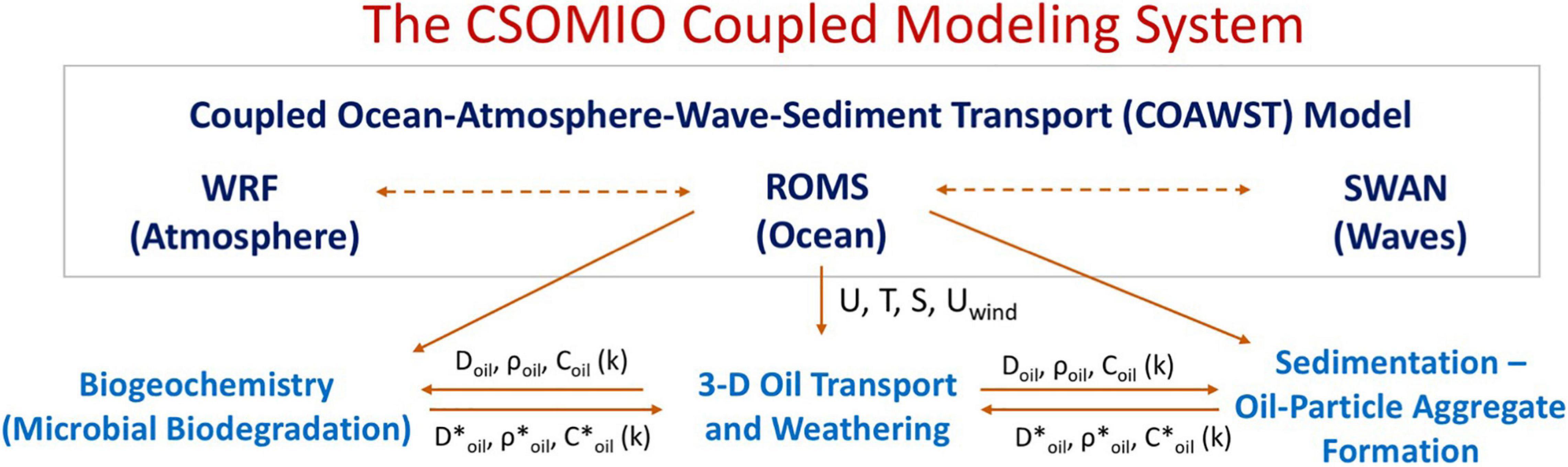
Figure 1. Chart diagram presenting the CSOMIO modeling system and interaction among the components.

This paper presents the first three-dimensional model that couples hydrodynamics, oil weather and transport, microbial feedbacks, and sedimentation for a realistic application of an oil spill scenario. In the following sections, description of the CSOMIO modeling components and the two-way Lagrangian-Eulerian mapping is provided. The paper also presents results of test experiments with the new modeling system. Test simulations are conducted with the model configured for the northern Gulf of Mexico region near the location of the DWH oil spill. Details of the model parameters and forcing fields are listed in Table 1. Test simulations have been performed with online and offline configurations of the CSOMIO model. Specific details of the model configuration for particular tests are provided in the text. A list of variables used in the test is given in Table 2.

TABLE 1

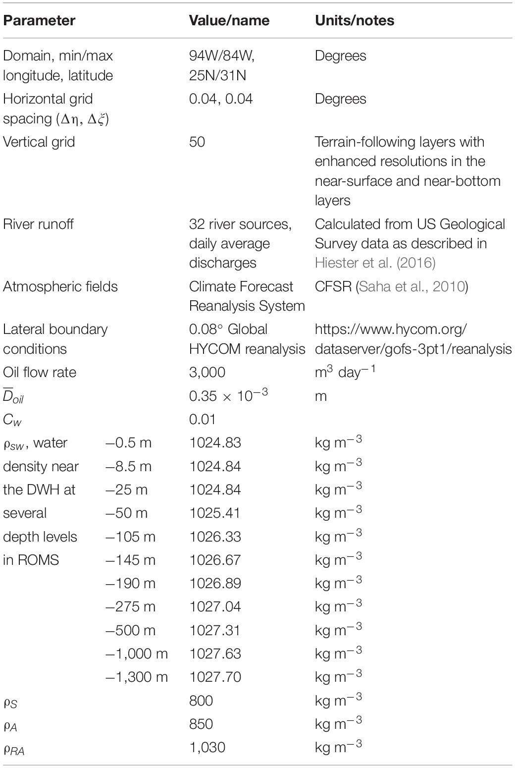
Table 1. Model parameters for test simulations.

TABLE 2

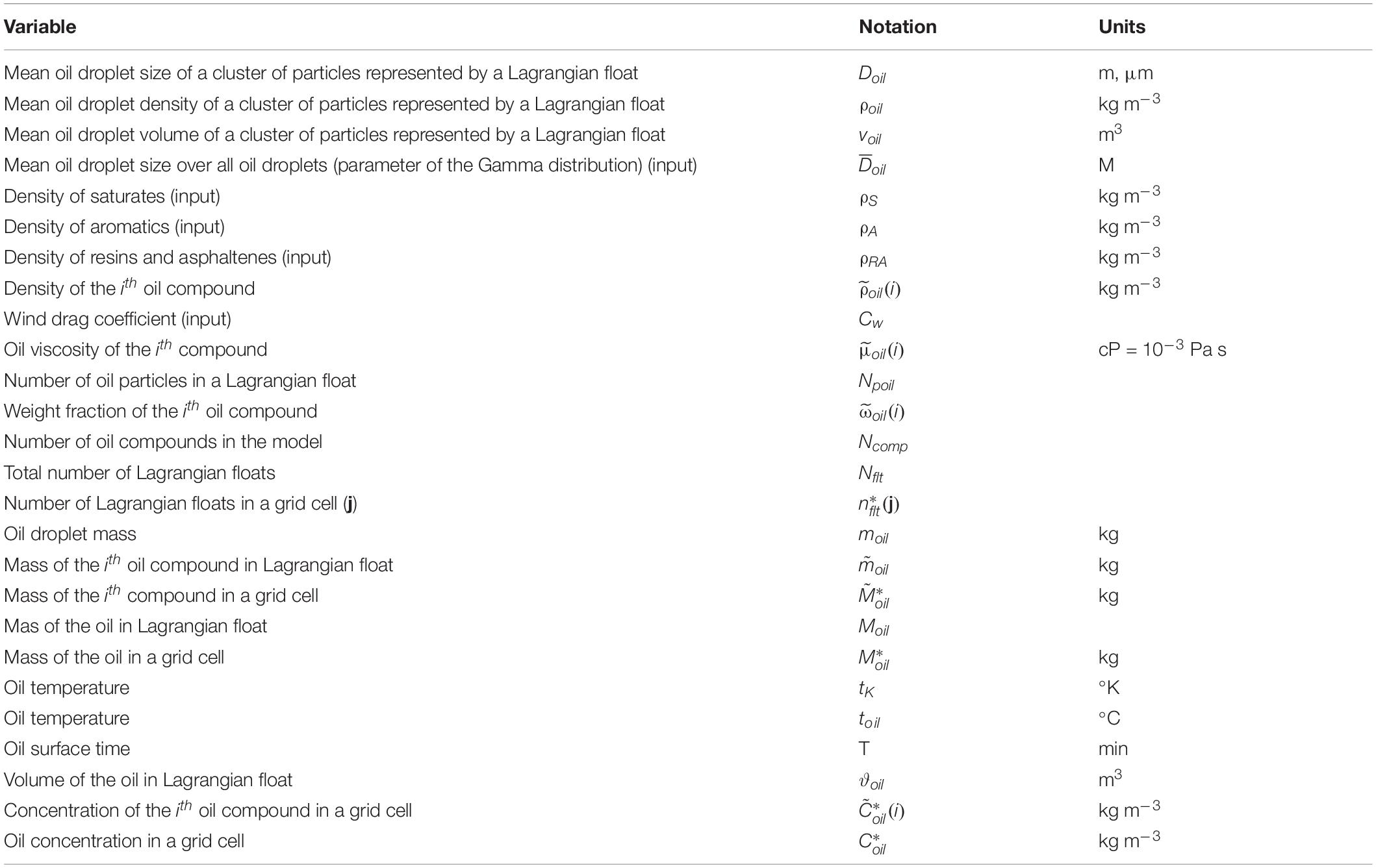
Table 2. List of variables, their notations and units.

CSOMIO Coupled Ocean-Oil-Sediment-Biology Model

Oil Transport and Weather Model (OTWM)

The Oil Transport and Weather Model (OTWM) is a particle trajectory simulation system coupled to the hydrodynamic model ROMS. The OTWM is a far-field model simulating three-dimensional movement of oil. In general, oil released from a wellhead contains high concentration of gasses and leaves the wellhead at high speed. Due to different temporal and spatial scales, a special class of models (so-called near-field models) is employed to simulate processes of a fast rising of mixture of oil, gas, and seawater and formation of oil droplets occurring within several to ∼100 m (trap height) above the wellhead (Socolofsky et al., 2011, 2016; Paris et al., 2012). After gas-saturated components leave the plume, the dynamics of the plume, represented as a mixture of oil droplets, are then controlled by the buoyant velocity and ocean currents and can be simulated by far-field models (Yapa and Zheng, 1997; Lardner and Zodiatis, 2017; Bracco et al., 2020; Perlin et al., 2020).

The OTWM simulates movement of oil using a Lagrangian approach that describes the oil dynamics through advection and diffusion of individual elements (hereinafter referred to as “floats” following terminology used in ROMS), each representing a cluster of oil droplets (section “Representation of Oil in the OTWM”). The code employs a Lagrangian float module in ROMS with added vertical velocity of oil particles in the water column calculated from oil characteristics (section “Buoyant Velocity of Oil Droplets”) and wind-driven surface drift (section “Wind Drift of Surfaced Oil”). The chemical composition of oil is described in terms of three classes of compounds: saturates, aromatics, and heavy oil (resins and asphaltenes). For each Lagrangian element, the OTWM simulates time-evolving changes of the following oil characteristics: location (depth and horizontal coordinates), density (changing chemical compounds), and mean size of oil droplets. The OTWM also incorporates the impact of surface wind drift and weathering (evaporation) effects.

Representation of Oil in the OTWM

The volume of oil released during an oil spill event is discretized by Lagrangian floats. The number of floats (N_flt), their release locations, duration, and discharge frequency are specified by the user. Each float represents a finite number (a cluster) of individual oil particles characterized by mean oil droplet size (D_oil) and density (ρ_oil).

Oil Droplet Size

During subsurface oil spills, oil forms droplets of varying sizes. Oil droplet size is an important characteristic of oil that controls the buoyancy and ascent rate of the droplet (section “Buoyant Velocity of Oil Droplets”). Oil droplets have a wide range of sizes observed in the marine environment and laboratory experiments (e.g., Li et al., 2008). The distribution of oil droplet sizes during the DWH spill event is uncertain due to several oil releases through kink holes of different sizes during the pre-riser cut vs. a single release during the post-riser cut, spill exit velocity, and unknown effects of dispersant applied directly during the spill. The study by Spaulding et al. (2017) suggests that before the pre-riser cut time (June 3, 2010) small droplets formed due to mechanical dispersion driven by high exit velocities at the kink holes, and dispersant application had a smaller effect. During the post-cut period, oil dispersion was mainly caused by the application of dispersants, which were more effectively applied. Spaulding et al. (2017) indicates that treated oil would have droplet sizes ranging from 20 to 500 μm, whereas untreated oil would have oil droplet sizes from 1,000 to 10,000 μm. Analysis of samples collected in the water column in the vicinity of the wellhead in June 2010 from the R/V Jack Fritz 3 cruises (Davis and Loomis, 2014) showed that oil droplets that remained in the water column by the time the sampling occurred were ≤ 300 μm (Spaulding et al., 2017).

In the OTWM, the oil droplet sizes (D_oil) are randomly generated for individual Lagrangian floats using a Gamma distribution (Vilcáez et al., 2013)

$$f(D_{oil};\mathrm{\alpha },\mathrm{\lambda })=\frac{{\mathrm{\lambda }}^{\mathrm{\alpha }}{\left(D_{oil}\right)}^{\mathrm{\alpha }-1}{e}^{-\mathrm{\lambda }{D}_{oil}}}{\mathrm{\Gamma }(\mathrm{\alpha })},(1)$$

where α is a free parameter that controls the spread of the Gamma probability density function. In the experiments described in this paper, α=4.94 corresponding to the coefficient of variation 0.4 in Vilcáez et al. (2013); λ is another parameter of the Gamma distribution determined as $\mathrm{\lambda }=\mathrm{\alpha }/{\overline{D}}_{oil}$, where ${\overline{D}}_{oil}$is specified by the user in the input file. In the test experiments presented in this paper, ${\overline{D}}_{oil}$ = 350 μm unless mentioned otherwise. The specified parameters are used to randomly generate D_oil(i) for the Lagrangian floats i = 1, …, N_flt (Figure 2A). In this particular set of D_oil(i), the maximum oil droplet size is 1,429 μm and the minimum size is 9 μm. Note that the model assumes a minimum droplet size of 0.19 μm, which is a size at which droplets are generally dissolved (North et al., 2015).

FIGURE 2

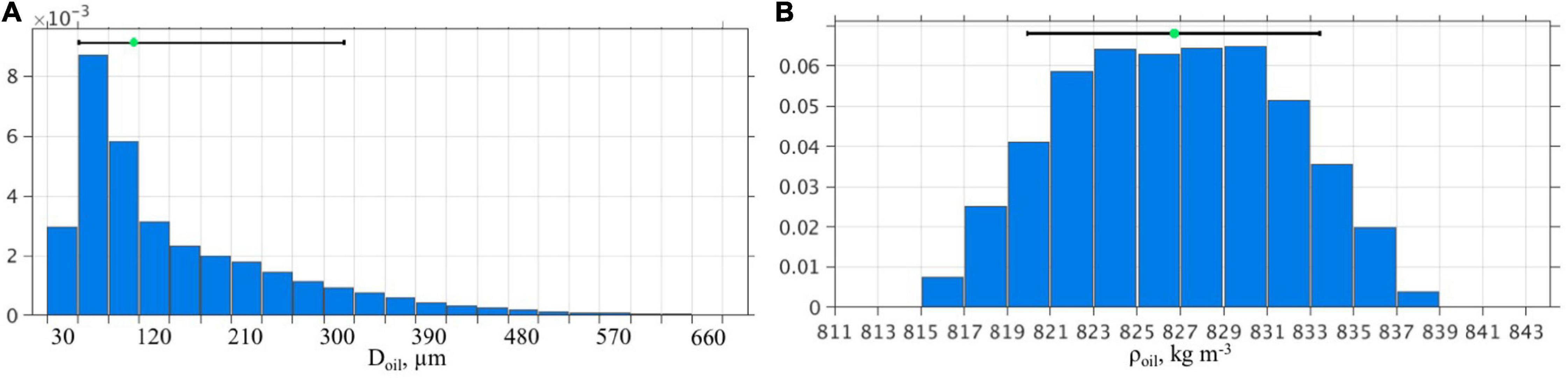
Figure 2. Histograms showing the distributions of initial oil particle sizes (A) and densities (B) for the Lagrangian floats in CSOMIO experiments. The black horizontal lines show the interdecile range and the green bullet is the median.

Oil Droplet Density

Crude oil is a mixture of thousands of hydrocarbons ranging from smaller, volatile compounds to large, non-volatile compounds (Speight, 2007). Properties of oil, such as viscosity, density, specific gravity, solubility, and flash point, are determined by the oil chemical structure (Fingas, 2015a). A common classification of oil chemical structure is given in terms of four compounds: saturates, aromatics, resins, and asphaltenes (SARA) (e.g., Klein et al., 2006).

The OTWM is developed for a multi-compound representation of oil chemical structure. The number of compounds and their characteristics (densities, weight fraction) are specified by the user. In the presented experiments, the OTWM was set for three oil compounds representing saturated, aromatic, and heavy polar compounds, including resins and asphaltenes (SAR+A). Compositional information for Macondo oil was deduced from water column samples collected at the Macondo well in June 2010 (Reddy et al., 2012, 74% saturated, 16% aromatics, and 10% polar hydrocarbons). These values are used as the mean fractions of the compounds in generating densities of the oil particles densities (ρ_oil), as follows.

The compositional structure of the oil is prescribed to each Lagrangian float by randomly assigning the weight fractions of aromatics (${\tilde{\mathrm{\omega }}}_A$) and heavy polar hydrocarbons (${\tilde{\mathrm{\omega }}}_{RA}$). The fractions are derived from uniform distributions as ${\tilde{\mathrm{\omega }}}_A\sim U(0.085,\mathrm{\hspace{0.25em}0.235})$ and ${\tilde{\mathrm{\omega }}}_{RA}\sim U(0.06,\mathrm{\hspace{0.25em}0.14})$ yielding the fraction of saturates as ${\tilde{\mathrm{\omega }}}_S=1-({\tilde{\mathrm{\omega }}}_A+{\tilde{\mathrm{\omega }}}_{RA})$. Note that by doing so, the mean fraction of each compound matches the estimates of the compositional structure of Macondo oil reported in Reddy et al. (2012).

The oil droplet density is estimated using the mixing rule for a regular solution (Yarranton et al., 2015) as

$$\frac{1}{{\mathrm{\rho }}_{oil}}=\frac{{\tilde{\mathrm{\omega }}}_S}{{\tilde{\mathrm{\rho }}}_S}+\frac{{\tilde{\mathrm{\omega }}}_A}{{\tilde{\mathrm{\rho }}}_A}+\frac{{\tilde{\mathrm{\omega }}}_{RA}}{{\tilde{\mathrm{\rho }}}_{RA}}=\sum _{i=1}^{N_{comp}}\frac{{\tilde{\mathrm{\omega }}}_i}{{\tilde{\mathrm{\rho }}}_i},(2)$$

where i is float index (i = 1, …, N_flt), ${\tilde{\mathrm{\rho }}}_S,{\tilde{\mathrm{\rho }}}_A,$ and ${\tilde{\mathrm{\rho }}}_{RA}$ are densities of the individual compounds specified in the input file, N_comp is the number of oil compounds in the model (3 in this model configuration). In the numerical experiments presented here, the following values were used ρ_S = 800 kg m^–3, ρ_A = 850 kg m^–3, and ρ_RA = 1,030 kg m^–3. The densities are normally distributed across the floats (Figure 2B), with the mean value (826.2 kg m^–3) close to the mean oil droplet density of 820 kg m^–3 reported by Reddy et al. (2012). Note that the compound densities do not change during the simulation. Instead, weight fractions are changed during the weathering, biodegradation and sedimentation processes resulting in changing (increasing) densities of the oil particles (sections “Surface Evaporation of Oil,” Sediment Model,” and “Biogeochemical Model”).

Buoyant Velocity of Oil Droplets

In the subsurface layers, vertical velocity of oil (w_oil) in the OTWM is a combination of hydrodynamic vertical velocity, random component (approximating diffusion) and buoyant velocity (w_b) driven by the buoyancy force in the water column. Two approaches (the two-equation algorithm and integrated algorithm) for calculating the buoyant velocity of oil droplets are implemented in the OTWM based on Zhang and Yapa (2000). The choice of the algorithm is specified by the user.

The Two-Equation Algorithm

The two-equation algorithm for the oil droplet buoyant velocity is based on the Stokes law that is valid for a small Reynolds number

$$Re=\frac{{\mathrm{\rho }}_{sw}{D}_{oil}{w}_b}{{\mathrm{\mu }}_{sw}},(3)$$

where ρ_sw is ambient sea water density (Table 1) and μ_sw is dynamic viscosity of ambient sea water. Two equations for oil droplet buoyant velocities are used for different Re. The choice of the equations is based on a critical diameter d_c

$$d_c=\frac{9.52{\mathrm{\mu }}_{sw}^{2/3}}{{\left(g{\mathrm{\rho }}_{sw}\mathrm{△}\mathrm{\rho }\right)}^{1/3}},(4)$$

where g is the gravitational acceleration and △ρ = ρ_sw − ρ_oil.

The buoyant velocity is calculated as

$$w_b={\{}_{{\left(\frac{8g{D}_{oil}\mathrm{\Delta }\mathrm{\rho }}{3{\mathrm{\rho }}_{sw}}\right)}^{1/2},D_{oil}\ge d_c}^{\frac{g{D}_o^{2}il\mathrm{\Delta }\mathrm{\rho }}{18{\mathrm{\mu }}_{s}w},D_{oil}<d_c}(5)$$

The Integrated Algorithm

For the integrated approach, the buoyant velocity is a function of the particle shape that is related to the particle size (equivalent particle diameter Doil) grouped in to three categories.

(1) For a spherical shape (D_oil≤1 mm), the buoyant velocity is calculated as

$$w_b=\frac{Re{\mathrm{\mu }}_{sw}}{{\mathrm{\rho }}_{sw}{D}_{oil}}(6)$$

(2) Ellipsoid shape (1 mm < D_oil ≤ 15 mm).

The criteria for this regime are M < 10 − 3 and E0 < 40. The coefficients M and E0 are defined as

$$M=\frac{g{\mathrm{\mu }}_s^{4}w\mathrm{\Delta }\mathrm{\rho }}{{\mathrm{\rho }}_{sw}^2{\mathrm{\sigma }}_{ow}^3}(7)$$

$$E_0=\frac{g\mathrm{△}\mathrm{\rho }{D}_{oil}^2}{{\mathrm{\sigma }}_{ow}}(8)$$

where σ_ow is oil - water interfacial tension determined as a function of water temperature (t°C) by Peters and Arabali (2013)

$${\mathrm{\sigma }}_{ow}=(0.1222t+32.82)\cdot {10}^{-3}(9)$$

The buoyant velocity is determined as

$$w_b=\frac{{\mathrm{\mu }}_{sw}}{{\mathrm{\rho }}_{sw}{D}_{oil}}{M}^{-0.149}\left(J-0.857\right)(10)$$

where

$$J={\{}_{3.42H{}^{0.441},H>59.3}^{0.94H{}^{0.757},\mathrm{\hspace{0.33em}\hspace{0.33em}\hspace{0.33em}\hspace{0.33em}\hspace{0.33em}\hspace{0.33em}\hspace{0.33em}2}<H\le 59.3}(11)$$

$$H=\frac{4}{3}{E}_0{M}^{-0.149}{\left(\frac{{\mathrm{\mu }}_w}{{\mathrm{\mu }}_{sw}}\right)}^{-0.14},(12)$$

where μ_sw is dynamic viscosity of sea water [kg⋅(m⋅s)^–1] determined by Sharqay et al. (2010)

$${\mathrm{\mu }}_{sw}={\mathrm{\mu }}_w(1+A\cdot S+B\cdot S^2)(13)$$

$$A=1.541+1.998\cdot {10}^{-2}t-9.52\cdot {10}^{-5}{t}^2(14)$$

$$B=7.974-7.561\cdot {10}^{-2}t+4.724\cdot {10}^{-4}{t}^2(15)$$

where S is salinity (g⋅kg^–1), and μ_w is dynamic viscosity of pure water given as

$${\mathrm{\mu }}_w=4.2844\cdot {10}^{-5}+{\left[0.157{\left(t+64.993\right)}^2-91.296\right]}^{-1}(16)$$

(3) For a spherical cap (large size droplets, E₀ > 40), the buoyant velocity is

$$w_b=0.711\sqrt{\frac{g{D}_{oil}\mathrm{△}\mathrm{\rho }}{{\mathrm{\rho }}_{sw}}}(17)$$

Note that for the presented OTWM simulations the spherical cap regime is not used due to smaller oil droplet sizes (Figure 2A).

Sensitivity Experiments With Buoyant Velocity Algorithms

The buoyant velocity of an oil particle is important because it determines the ascent rate of the particles and thus, the surface time and the duration of time during which the particle is subject to subsurface biodegradation processes and interaction with suspended sediments.

Sensitivity simulations employing the two algorithms for the oil droplet buoyant velocity are performed in order to test the sensitivity of the simulated oil vertical velocity to the choice of the algorithm (Figure 3). The simulations are conducted with OTWM coupled to ROMS and neither biogeochemical nor sediment-OPA modules being activated. Except for the buoyant velocity algorithms, the experiments are identical. To account for near-field dynamics of the turbulent plume and multiple release locations during the pre-cutting of the broken riser, Lagrangian floats are released at several locations within a few hundred meters around the wellhead (88.36°W and 27.738°N) at ∼1,400 m. The simulations last 7 days with Lagrangian floats released every 1.29 min at each location. A total of 40,000 floats are released during this simulation.

FIGURE 3

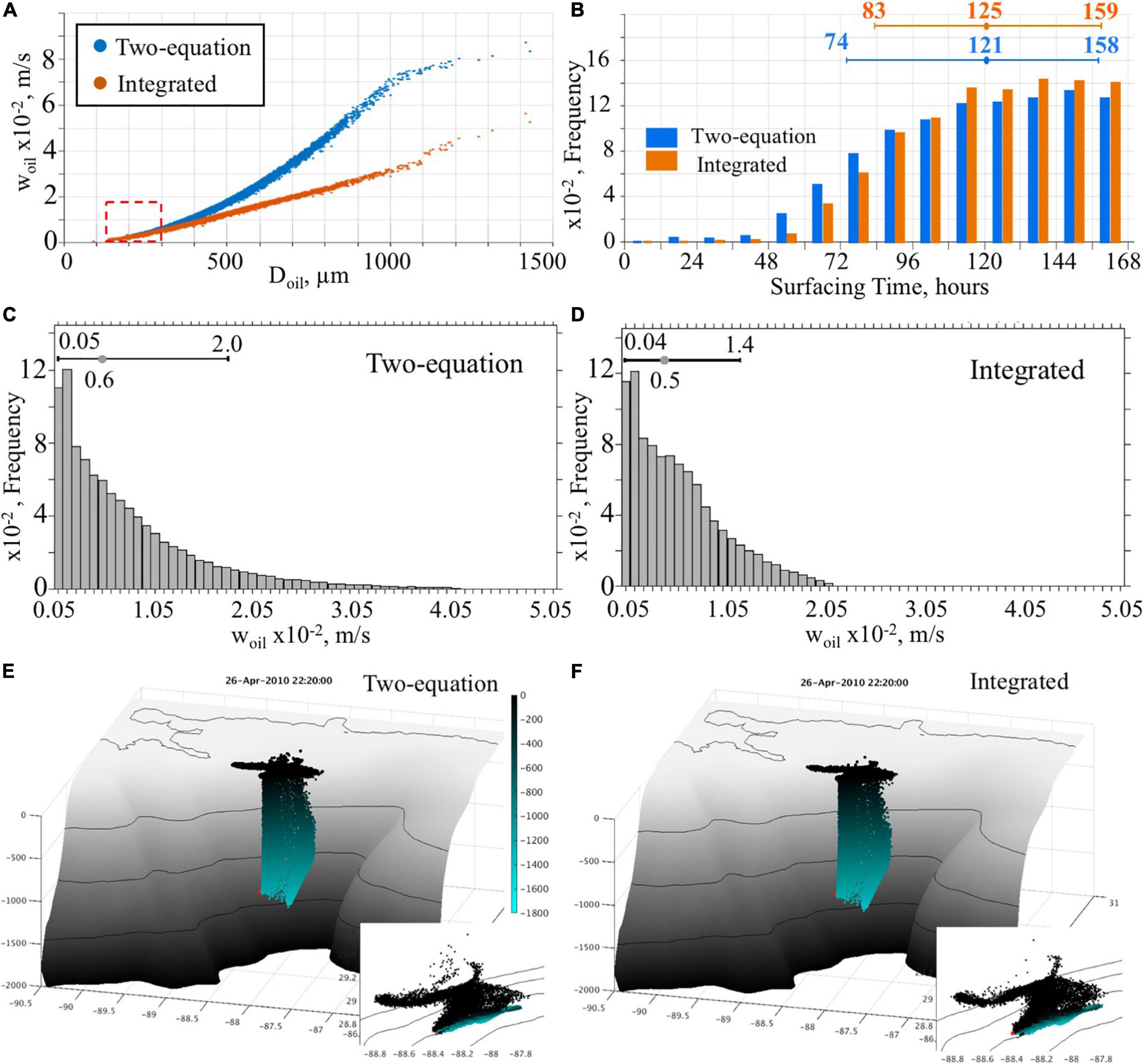
Figure 3. (A) oil droplet vertical velocity vs. oil droplet size from OTWM simulations using two-equation and integrated algorithms of buoyant velocity. The red dashed box indicates the interdecile region for D_oil from Figure 2A. (B) The surfacing time (hours after release) of oil droplets estimated from the 7 day test simulations with two algorithms for buoyant velocity. At the top, the median, 10th and 90th percentiles are presented. (C,D) Histograms showing w_oil distribution in the OTWM simulations using two-equation (left) and integrated (right) algorithms of buoyant velocity. (E,F) 3-dimensional distribution of the Lagrangian floats in the water column in the OTWM simulations using different formulations of buoyant velocities after 7 days of the simulation. The insets show the float positions projected onto the sea surface plane. Colors designate particles’ depth in the water column.

The vertical velocities of oil (w_oil) from the two simulations are similar for the oil droplets smaller than ∼300 μm but are different for the larger oil particles (Figure 3A). The two-equation algorithm produces notably faster ascent velocities than the integrated algorithm for the larger oil droplets with D_oil > 300 μm. In the presented simulations, the median D_oil is ∼100 μm and the 90th percentile is ∼310 μm (Figure 2A). Thus, simulated vertical speed is similar in the experiments employing different algorithms for ∼90% of the oil particles (Figures 3C,D).

The difference in w_oil for oil particles affects the time required for Lagrangian floats to reach the surface (Figure 3B). For the range of oil particles’ sizes considered in the test simulation, the difference in an oil surfacing time from the two simulations is small (the medians are 125 and 121 h for the integrated and two-equation algorithm, respectively). The simulation with the two-equation algorithm predicts the fastest oil surfacing time ∼6–12 h earlier than in the experiment using the integrated formula. In the two-equation simulation, the first group of oil floats reaches the surface in the first 6–12 h, whereas this is 12–24 h in the simulation with the integrated algorithm. Nevertheless, qualitatively the difference between the experiments is barely noticeable in the three-dimensional distribution of the oil particles (Figures 3E,F).

The surfacing time of the first oil during the DWH is uncertain. Available reports on the timeline of the oil spill indicate that no leaking oil was observed on the surface until the morning of April 23, 2010, i.e., roughly 24 h after the oil rig sank (U.S. Senate Committee on Environment and Public Works, 2010). Hence, the surfacing time of oil estimated from both test simulations look reasonable.

Wind Drift of Surfaced Oil

As oil surfaces, it becomes subject to direct atmospheric forcing. This is expressed as wind drift, or the advective velocity of oil particles due to wind. This correction of the surface oil velocity is commonly used in surface oil drift models to compensate for coarse vertical representation of surface velocity in hydrodynamic models (Abascal et al., 2009). Following MacDonald et al. (2016), the oil particles trajectories at the surface are computed as a superposition of advective velocity and turbulent diffusion

$$\frac{d\mathbf{\text{x}}}{dt}={\mathbf{\text{u}}}_a(\mathbf{x},t)+{\mathbf{\text{u}}}_d(\mathbf{x},t),(18)$$

where u_a is the advective (oil drift) velocity and u_d is the diffusive velocity. The advective velocity is calculated as a linear combination of the surface ocean currents, 10 m wind vector and waves

$${\mathbf{\text{u}}}_a={\mathbf{\text{u}}}_c+C_w\left|{\mathbf{\text{u}}}_{10}\right|\mathbf{\Theta }+C_s{\mathbf{\text{u}}}_s,(19)$$

where u_c is the ocean surface current velocity of seawater estimated from the topmost grid layer of an ocean model, C_w is the wind drag coefficient, u₁₀ is the wind velocity 10 m above the sea surface, Θ is a unit vector directed at an angle θ relative to the wind (wind deflection angle), Cs is the wave coefficient and u_s is the wave-induced Stokes drift. Typically, the wind drag coefficient varies from 0.025 to 0.044 (American Society of Civil Engineers Committee on Modeling Oil Spills, 1996). The wind deflection angle is typically 20 degrees clockwise from the wind direction (in the Northern Hemisphere). The OTWM uses wind-dependent formulation for the wind deflection angle (Samuels et al., 1982)

$$\mathrm{\theta }=-{25}^{o}exp\left(-{10}^{-8}\left|{\mathbf{\text{u}}}_{10}\right|/{\mathrm{\nu }}_{k}g\right),(20)$$

where ν_k is the kinematic viscosity of the sea water.

In many applications, wind and wave effects are combined and both represented by the wind drag coefficient. For example, under light wind conditions without breaking waves Reed et al. (1994) found that C_w = 0.035 provided realistic simulation of oil slick drift in offshore areas. In the presented numerical experiments, wave effects are not explicitly added to u_a. It should be noted, however, that the value of C_w needs to be adjusted based on the accuracy of representation of true (“skin”) surface currents (a current within a thin surface layer whose thickness is on the order of oil thickness) by u_c. In many applications, u_c is the near-surface velocity from a hydrodynamic model and, as such, represents velocity averaged over the top model layer, whose thickness exceeds the thickness of the surface current. Thus, u_c may substantially differ from the true “skin” surface velocity. This is demonstrated by the study of Morey et al. (2018) who analyzed trajectories of satellite-tracked surface drifters in the northern Gulf of Mexico and found a notable velocity shear within the upper meter of the ocean. Therefore, u_c needs correction. However, the correction strongly depends on the vertical resolution of the near-surface layers in the model. Models with finer vertical surface layers need weaker adjustments, and C_w and the turning angle should be smaller (van der Mheen et al., 2020). In the OTWM, C_w is specified by the user and provided in the float input file. The wind effect can be eliminated by setting Cw to 0 in the float input file. Another option is to undefine the wind drift in the preprocessing definitions. The second option is required if a simulation is performed without wind (or atmospheric) forcing. In the presented experiments for the given ROMS configuration, C_w = 0.01. For future development of the CSOMIO model, C_w could be parameterized as a function of the thickness of the uppermost model grid layer, which is represented by u_c.

Turbulent diffusive velocities u_d are approximated as random fluctuations defined based on “random walk” (Garcia-Martinez and Flores-Tovar, 1999; Lonin, 1999; Isobe et al., 2009)

$${\mathbf{\text{u}}}_d=U_d\varsigma exp\left(i2\mathrm{\pi }\varsigma \right),(21)$$

where ς is a random variable from the standard Gaussian distribution and

$$U_d=\sqrt{\frac{c_0{K}_h}{\mathrm{△}t}},(22)$$

where c₀ is a constant, K_h is the horizontal diffusion.

Surface Evaporation of Oil

Evaporation dominates the early stage of oil weathering at the ocean surface. Historical estimates of oil evaporation from the ocean surface range from 20 to 80% of their volume during the first few days. The National Incident Command estimated that 25% of the total oil released evaporated during the DWH spill (Lubchenco et al., 2010). Evaporation processes are faster than dissolution and degradation processes (i.e., oxidation and biodegradation).

Physical and chemical processes that control oil evaporation cannot be described as a single relationship due to the complexity of oil’s chemical structure and numerous factors affecting physics and the chemistry of oil compounds (Fingas, 1995, 1996). In practice, evaporation curves are empirically derived for particular types of oil from field observations and laboratory tests. Oil evaporation rates vary greatly with time, and individual compounds can have drastically different evaporation rates. The most intense evaporation typically occurs during the first 24 h as lighter compounds evaporate, after which the overall evaporation rate decreases. During this process, light oils change their chemical and physical properties becoming more viscous. Heavy oils become solid-like and may form tar balls and tar mats (Fingas, 2012; Zodiatis et al., 2017).

Several algorithms are available for modeling oil evaporation. French-McCay and Payne (2001) presented a pseudo-component approach to simulate oil weathering. Using this approach, the oil is treated as seven pseudo-components defined by distillate cut and compound classification (three aromatic fractions, three aliphatic fractions, and one non-volatile fractions). Stiver and Mackay (1984) presented a method known as the “evaporative exposure approach.” Based on laboratory experiments and analytical considerations, Fingas (2012, 2015b) suggested a different approach for oil evaporation modeling. In contrast to the previous two approaches, he argued that oil evaporation is diffusion limited by the oil itself and hence it is not air-boundary-layer regulated. Experiments demonstrated that evaporation rates for oils, and even a light product gasoline, were not significantly increased with increasing wind speed. Also, the experiments showed no correlation between oil area and evaporation rate (in contrast to air-boundary-layer regulated liquids, such as water). The experiment showed that oil temperature was the main factor determining the evaporation rate.

In the OTWM, a multi-component approach based on Fingas (2012) is implemented to simulate evaporation of the oil at the ocean surface. This approach is necessary for tracking changes in oil composition, density, and oil particle sizes. The evaporation algorithm is activated when a Lagrangian float is at the surface. The percentage of evaporated oil is calculated for each compound (i) separately

$$E_{oil(i)}=\left[E+0.675+0.045\left(t_{oil}-15\right)\right]\text{ln}(T),(23)$$

where t_oil is oil temperature (taken as ambient ocean temperature), T is the cumulative time of the oil at the surface in minutes (where T > 1.0 to avoid negative evaporation), and E is the evaporation equation parameter given by

$$E=15.4-14.5{\mathrm{\rho }}_i+2.58{\left({\tilde{\mathrm{\mu }}}_{oil}(i)\right)}^{-1},(24)$$

where ρ_i is density of the i^th oil compound (kg m^–3) and ${\tilde{\mathrm{\mu }}}_{oil}(i)$ is dynamic viscosity (cP) of the i^th oil compound. The oil dynamic viscosity (in cP) is calculated as Sanchez-Minero et al. (2014)

$${\mathrm{\mu }}_{oil(i)}=a\cdot exp\left(b{t}_K^{-3}\right),(25)$$

where t_K is oil temperature (in °K) and coefficients a and b are correlating parameters in the viscosity correlation

$$a=3.9\times {10}^{-5}AP{I}^3-4.0\times {10}^{-5}$$

$$AP{I}^2+0.1226API-0.7626,(26)$$

$$b=9.1638\times {10}^{9}AP{I}^{-1.3257}.(27)$$

In the above formulas, API is the American Petroleum Institute gravity calculated for the oil compounds as

$$API=\frac{141.5}{SG}-131.5,(28)$$

where SG is specific gravity of the oil.

For heavy oil compounds (API < 10.0), the oil viscosity is estimated using one of the methods discussed in Bahadori et al. (2015)

$${\mathrm{\mu }}_{oil(i)}={10}^a{t}_K^b,(29)$$

where the coefficients are

$$a=-71523API+22.13766,(30)$$

$$b=0.269024API-8.26.(31)$$

An example of evaporation curves for the three compounds used in the presented OTWM (saturates, aromatics and resins-asphaltenes) calculated using Eqs. (23)–(31) is shown in Figure 4A.

FIGURE 4

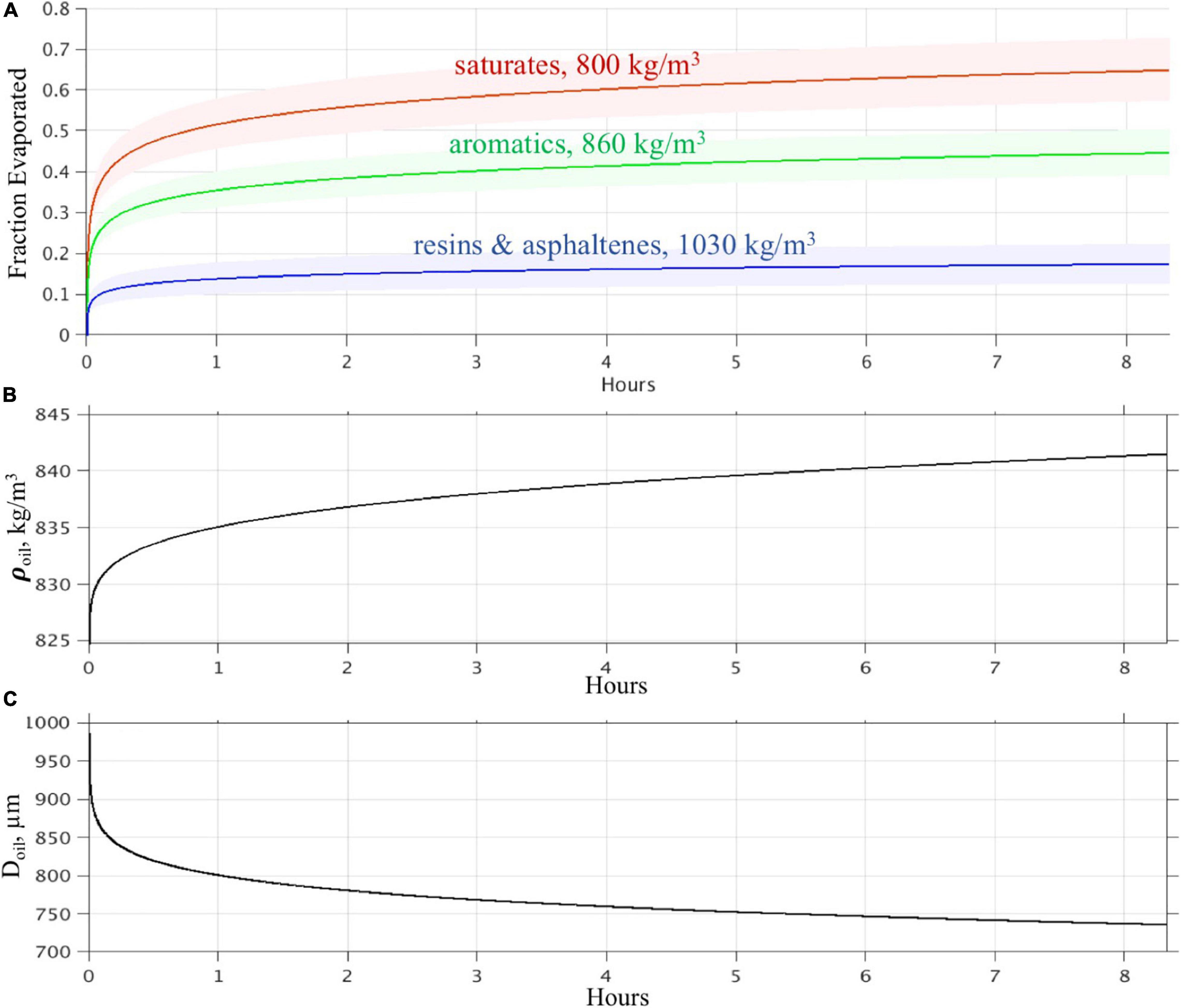
Figure 4. (A) Evaporation curves for saturates, aromatics, and heavy oil compounds calculated using the approach discussed in section “Surface Evaporation of Oil.” The densities of the compounds are listed in the figure. The solid lines are the evaporation curves for 25°C. The shades highlight the range of the evaporation curves calculated for temperatures from 15 to 35°C for each compound. The horizontal axis is hours. (B) Change of the oil droplet density due to evaporation. (C) Change of the oil droplet size due to evaporation.

After each time step, changes driven by evaporation in the characteristics of oil droplets are updated as follows. The new weight fraction of the i^th oil compound is

$${\tilde{\mathrm{\omega }}}_{oil}^{\left(k+1\right)}\left(i\right)=\frac{{\tilde{m}}_{oil}^{\left(k+1\right)}(i)}{m_{oil}^{(k+1)}},(32)$$

where $m_{oil}^{(k+1)}$ is the updated mass of the oil particle (next time step k+1) and ${\tilde{m}}_{oil}^{\left(k+1\right)}(i)$ is new mass of the oil i^th compound in the oil particle given as

$${\tilde{m}}_{oil}^{\left(k+1\right)}(i)=\left(1-E_{oil}\left(i\right)\right){\tilde{m}}_{oil}^{\left(k\right)}(i).(33)$$

Here, ${\tilde{m}}_{oil}^{\left(k\right)}(i)$ is mass of the oil i^th compound at the time step k and the mass of the oil droplet is

$$m_{oil}^{(k)}=\sum _{i=1}^{N_{comp}}{\tilde{m}}_{oil}^{\left(k\right)}(i).(34)$$

The updated weight fraction (Eq. 32) for the individual compounds is used to update oil droplet densities (${\mathrm{\rho }}_{oil}^{(k+1)}$) using Eq. 2. Next, new values of the oil droplet mass and density are used to update oil droplet size (D_oil) by updating volume of the oil droplet first

$$v_{oil}^{(k+1)}=\frac{m_{oil}^{(k+1)}}{{\mathrm{\rho }}_{oil}^{(k+1)}},(35)$$

where $m_{oil}^{(k+1)}$ has been updated using new ${\tilde{m}}_{oil}^{\left(k+1\right)}(i)$ in Eq. 34. The new oil droplet size ($D_{oil}^{(k+1)}$) is derived from Eq. 35 assuming a spherical shape of the particle

$$D_{oil}^{(k+1)}=2{(\frac{3}{4\mathrm{\pi }}{v}_{oil}^{\left(k+1\right)})}^{1/3}.(36)$$

Examples of updated oil droplet density and size derived from the evaporation rate are shown in Figures 4B,C.

The impact of oil evaporation is demonstrated by looking at the distributions of oil droplet densities and sizes at the beginning and at the end of a test ROMS-OTWM simulation lasting 7 days (Figure 5). The analysis only includes the oil droplets that were on the surface for at least 4 days. The histograms demonstrate that after being subject to surface weathering (evaporation) oil particles become denser and smaller, as expected.

FIGURE 5

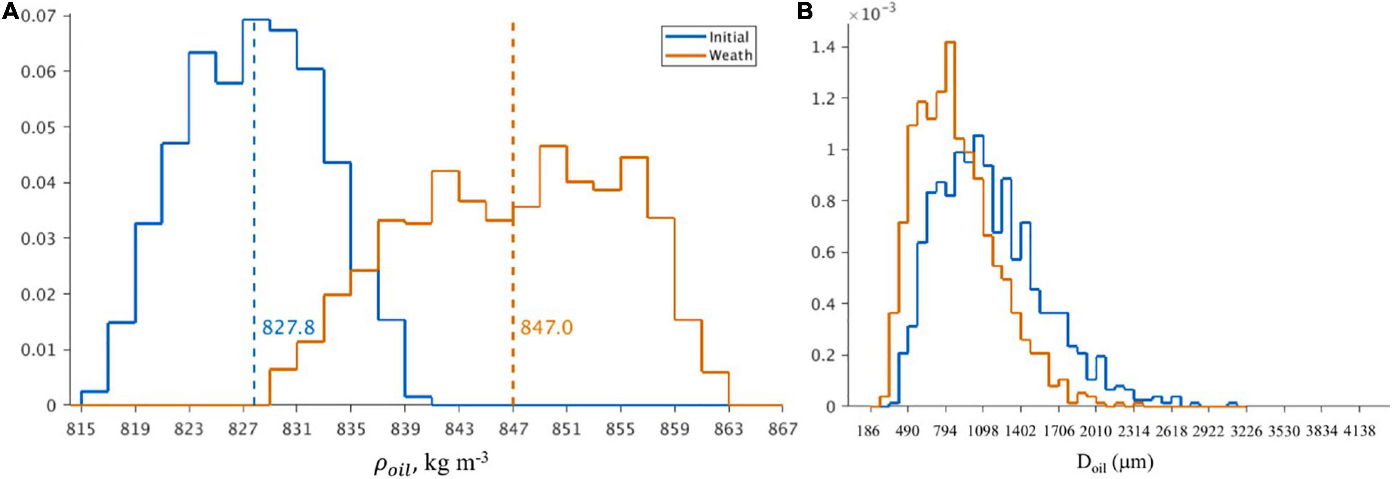
Figure 5. (A) Histograms of the oil droplet densities (ρ_oil) at the beginning (blue) and end (orange) of a 7 day ROMS-OTWM simulation that includes oil evaporation as the only loss term. Only particles that remained at the surface at least 4 days are considered. The vertical dashed lines indicate the mean. (B) Similar to (A) but for the oil droplet sizes (D_oil).

Sediment Model

To account for interactions between oil, and suspended sediment, the CSOMIO model built on the Community Sediment Transport Modeling System (CSTMS), which has previously been coupled with the ROMS hydrodynamic model (Warner et al., 2008), and has been used for simulations of sediment transport in the northern Gulf of Mexico (e.g., Xu et al., 2011; Zang et al., 2018; Harris et al., 2020). The sediment model represents a user-specified number of sediment classes. Properties for each class, which include diameter, density, settling velocity, and erosion rate parameter, are specified as input parameters and held constant throughout the simulation. Most applications of CSTMS have assumed non-cohesive sediment behavior (Warner et al., 2008). However, a more recent development added flocculation processes (Winterwerp et al., 2006; Manning et al., 2017) to the model (Sherwood et al., 2018) using a population balance model based on FLOCMOD (Verney et al., 2011), which uses a finite number of floc classes, and accounts for aggregation and disaggregation of flocs (Soulsby et al., 2013; Mehta et al., 2014) by moving sediment mass between the floc classes within each model grid cell. Implementation of the flocculation model requires additional model parameters including the fractal dimension (e.g., Kranenburg, 1994; Dyer and Manning, 1999), collision efficiency (e.g., Molski, 1989; Parsons et al., 2016; Hope et al., 2020), and fragmentation rate (see Sherwood et al., 2018).

The CSOMIO-sediment model extends the existing CSTMS to account for formation of OPA (Cui et al., 2020). Specifically, we adapted and modified FLOCMOD to incorporate an Oil-Particle-Aggregate Module (OPAMOD) within the CSTMS and added a new type of tracer to represent OPAs. OPAMOD uses the oil characteristics (droplet size, density, and concentration) and the suspended sediment characteristics (diameter, density, and concentration) to calculate the formation or growth of OPAs in the water column. At the end of flocculation process, concentrations of suspended sediment, oil, and OPAs are updated. OPAMOD included interactions between oil droplets and sediment flocs, oil droplets and OPAs, and sediment flocs and OPAs. The model was validated with a zero-dimensional simulation (Cui et al., 2020), which performed well when compared to laboratory data reported by Ye et al. (2020).

For the fully coupled, three-dimensional simulation, the sediment model used three cohesive sediment classes (one representing seabed material, two representing sediment delivered by the Mississippi River); and four OPA classes. The properties are shown in Table 3. The suspended sediment concentration for seabed mud class was initialized with 0.01 kg m^–3 within the bottom grid cells. The sediment concentrations from river input were extracted from a realistic simulation, which used riverine discharge from USGS gauge data (Harris et al., 2020). In OPAMOD, the fractal dimension was assumed to be 2.39. The fractal dimension of 2.39 was obtained using model calibration simulations to match laboratory results that studied the formation of OPA (Cui et al., 2020; Ye et al., 2020). The collision efficiency was set to 0.55 for the interaction between oil and sediment particles, and 0.35 for the interaction between sediment and OPAs, following Bandara et al. (2011). For the configuration presented in this paper, resuspension was neglected by defining a high critical shear stress for sediment. Resuspension was neglected in this study for multiple reasons. First, the main purpose of the sediment module in this coupled model is to capture the sedimentation of oil via the formation of OPAs. This sedimentation acts to enhance the delivery of oil to the seafloor, which is the effect we intended to represent. To consider the ultimate fate of the oil that is within OPA, over longer timescales, would require that we also account for resuspension of the OPA. Simulation of resuspension requires parameters for the critical shear stress for erosion. However, the critical shear stress of OPA is unknown, which makes the simulation of resuspension challenging.

TABLE 3

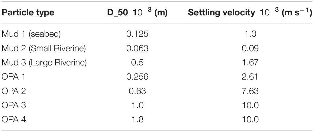
Table 3. Properties of sediment and OPAs.

Biogeochemical Model

The CSOMIO biological sub-model (BIO) is based on the ROMS Fennel et al. (2006) subroutine, which has been used extensively in the Gulf of Mexico and which provides a simple but complete biogeochemical model for the upper ocean. Although a number of improvements have been made to that model to better simulate the low oxygen zone extending beneath the Mississippi River plume (e.g., Laurent et al., 2012), the main CSOMIO goal was to incorporate the representation of the hydrocarbon-degrading microbes in open ocean regions. This has been achieved by incorporating elements of the Coles et al. (2017) gene-based model to integrate hydrocarbon-degrading bacteria. Three additional organisms are added to represent hydrocarbon-degrading bacteria. These are not randomly selected, but rather optimized as small cells of order 1 micron in diameter that degrade hydrocarbons while using nitrate or ammonium as a nitrogen source. Some additional model changes are also required. First, energy acquisition and nutrient acquisition are separated to allow for the use of pure carbon-based substrates as energy sources. To determine the yield on these hydrocarbons, theoretical approaches are used based on the Gibbs free energy of the reaction, following Reed et al. (2014), which was based on the work of Roden and Jin (2011). Conceptually, the yield is the ratio of the biomass increase to the hydrocarbon substrate uptake. Because the yield estimates are based on nutrient and substrate replete conditions, the maximum uptake rate of substrate is assumed to equal the maximum organismal growth rate divided by yield.

The three hydrocarbon groups in the CSOMIO model are intended to span a broad range of similar hydrocarbons with similar lability, and thus representative formula are computed for each group from the observed dissolved concentrations (Diercks et al., 2010; Mason et al., 2012; Reddy et al., 2012). The computational yield is then determined based on the redox reaction of each representative chemical compound (Saturates C₁₀H₂₂, yield = 5.7322 moles C biomass / mole of electron donors, Aromatics C₇H₈, yield = 3.3792 moles C biomass / mole of electron donors, heavy oil C₃₀H₅₂, yield = 15.6952 moles C biomass / mole of electron donors). Hydrocarbon uptake is not necessarily limited by nutrient availability. Organisms are able to use hydrocarbons for energy without adding biomass when nutrients are unavailable, however, mortality continues to reduce organismal biomass in the absence of active growth. Since these organisms are designed to be specialized as hydrocarbon degraders, there are no additional metabolic strategies available to the organisms for growth. In prior modeling efforts (Valentine et al., 2012), secondary substrates in the degradation of a hydrocarbon and the organisms that utilize them were added to a model, however, here the focus is solely on a single degradation step consistent with the available data for validation.

The equations modulating bacterial growth are

$$G_k={\mathrm{\mu }}_{max}{(1.066)}^T(37)$$

$${\mathrm{\mu }}_k=G_k\frac{S_k{k}_{sk}}{1+S_k{k}_{sk}}[{\left(\frac{N{H}_4{k}_{NH4}}{1+N{H}_4{k}_{NH4}}\right)}^{-1}\frac{N{O}_3{k}_{NO3}}{1+N{O}_3{k}_{NO3}}+$$

$$\frac{N{H}_4{k}_{NH4}}{1+N{H}_4{k}_{NH4}}],(38)$$

$$\frac{d{B}_k}{dt}={\mathrm{\mu }}_k{B}_k-m{B}_k(39)$$

$$\frac{d{S}_k}{dt}=-\frac{G_k}{Y_k}\frac{S_k{k}_{sk}}{1+S_k{k}_{sk}}{B}_k(40)$$

where μ_max is the maximum growth constant for each bacteria taxon. G_k is the organismal maximum growth rate given the ambient temperature conditions (T) following the same formulations used in the Fennel et al. (2006) model. μ_k then represents the actual growth rate of the organism once limited by both energy substrate S_k and the half saturation coefficient, k_s for that substrate, and by nitrogen availability as expressed through the combination of NO₃ and NH₄ concentration and their half saturation coefficients k_no3 and k_nh4. B_k is the organismal biomass, and m is the linear mortality coefficient. Absent grazing information on these bacteria we select a simple mortality function. Y_k is the yield determined by

$$Y_k=\frac{2.08-0.0211\mathrm{\Delta }{G}_{e^{-1}}}{24.6}.(41)$$

The energy yield G_e– is computed from the Gibbs free energy and the stoichiometry of the electron donor in the redox reaction, and the molecular weight of the microbial biomass is 24.6 g(C−molbiomass)−1, which is derived from the generic microbial biomass formula of CH_1.8O_0.5N_0.2 (Roels, 1981). The values of each coefficient are described in Table 4.

TABLE 4

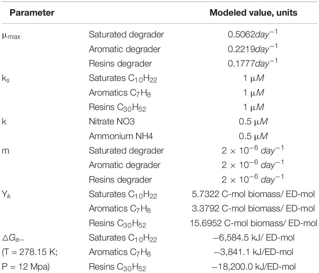
Table 4. Coefficients for the biochemical model.

Trace amounts of dissolved hydrocarbons in each group are maintained as Eulerian tracers in the model to allow for the maintenance of the hydrocarbon-degrading microorganisms. When Lagrangian oil is converted to the Eulerian framework, these two components are additive and the ratio is stored at each grid point. The bacteria convert hydrocarbons to biomass and carbon dioxide, and then the ratio is used to deconvolve the oil concentration back to the Lagrangian framework.

Online and Offline Configurations

The CSOMIO modeling system can be integrated in online and offline configurations. The advantage of the offline version is reduced computational time. To run offline, the physics base of the model should be integrated using ROMS and saved at an adequate frequency. Then, the tracer and oil can be run with the offline version of ROMS using these saved physics fields (u, v, ubar, vbar, zeta, and optionally the vertical salinity diffusion coefficient) to transport the tracer and oil instead of integrating all of the computations simultaneously, saving computational time. The offline ROMS version is modified so that when the appropriate flags are chosen, the physics base numerics are not run and instead the simulation reads in the saved velocity fields, then uses those values to run only the tracer and oil transport routines in ROMS. The physics fields are read in as climatology and forced fully for every grid node; they are linearly interpolated in time between available time steps just as climatology can be. Details of the computational savings and setup approach as well as details in the ROMS code modifications are available in Thyng et al. (2021).

Two-Way Eulerian-Lagrangian Mapping

The components of the CSOMIO model are linked together using a two-way Lagrangian-Eulerian mapping technique. The technique maps oil characteristics from a Lagrangian to Eulerian framework (Lagrangian-Eulerian mapping, LEM) in order to simulate oil biodegradation and sedimentation processes. After modification by the sedimentation and biogeochemical submodels, oil fields are mapped back to the Lagrangian framework (Eulerian-Lagrangian mapping, ELM) for the oil model. Implementation of the algorithm in the ROMS-OTWM code includes test subroutines verifying that the overall mass of oil is conserved during LEM and ELM. In order to distinguish variables in the Eulerian framework from the same variables in Lagrangian space, the Eulerian variables are denoted with an asterisk.

Lagrangian-Eulerian Mapping

Description of the Methodology

LEM consists of several steps. First, the Lagrangian floats whose position is given by a vector x_l (l = 1, …, N_flt) are clustered into groups bounded by grid cell faces, i.e., for every grid cell j = {j₁,j₂,j₃} a set of Lagrangian floats is defined as

$$S_{\mathbf{j}}=\{{\mathbf{\text{x}}}_{\mathbf{l}}\in {ℝ}^3:{||{\mathbf{\text{x}}}_{\mathbf{l}}-{\mathbf{\text{x}}}_{\mathbf{j}}^{(0)}||}_2<{||{\mathbf{\text{x}}}_{\mathbf{l}}-{\mathbf{\text{x}}}_{\mathbf{k}}^{(0)}||}_2,for\forall \mathbf{k}\ne \mathbf{\text{j}}\}(42)$$

where ${\mathbf{\text{x}}}_{\mathbf{j}}^{\left(0\right)}$ is a center point of the grid cell j and l is the float index.

Both the biogeochemical and sediment-OPA (OPAMOD) modules require information about the concentration of oil compounds. Hence, each compound is next mapped onto Eulerian space. The mass of oil compounds (index i) is integrated over the grid cells (j) where Sj is not empty,

$${\tilde{M}}_{oil}^{*}(\mathbf{j};i)=\sum _{l\in S(\mathbf{j})\ne \mathrm{\varnothing }}{\vartheta }_{oil}(l){\mathrm{\rho }}_{oil}(l){\tilde{\mathrm{\omega }}}_{oil}(i,l),(43)$$

where l is the float index and ϑ_oil(l) is the volume of oil represented by the l^th Lagrangian float. In general, ϑ_oil can vary across the floats if the oil discharge rate varies in time. In the presented experiments, the discharge rate is constant (3000 m³/day) and thus, initially ϑ_oil is the same across the floats being determined as

$${\vartheta }_{oil}=\frac{{𝔇}_{oil}}{{𝔇}_{flt}},(44)$$

where 𝔇_oil is the discharge of oil (specified by the user in the input file) and 𝔇_flt is the release frequency of the Lagrangian floats (specified in the input file). Concentrations of the oil compounds (${\tilde{C}}_{oil}^{*}$) in the grid cell (j) are

$${\tilde{C}}_{oil}^{*}(\mathbf{j};i)=\frac{{\tilde{M}}_{oil}^{*}(\mathbf{j};i)}{V_{grid}(\mathbf{j})},(45)$$

where V_grid is the volume of the grid cell. Mean oil droplet size in a grid cell required for the sediment-OPA model is obtained as

$$D_{oil}^{*}(\mathbf{j})=\frac{1}{n_{flt}^{*}(\mathbf{j})}\sum _{l\in S(j)}{D}_{oil}(l).(46)$$

where $n_{flt}^{*}(\mathbf{j})$ is the number of Lagrangian floats in the grid cell (j).

Test Simulations With LEM

A test simulation with the ROMS-OTWM and engaged LEM algorithm was performed. In the simulation, neither the biogeochemical nor sediment-OPA modules are activated, so that no changes in oil characteristics on the Eulerian framework are anticipated to occur. In this case, identical fields should be observed in Lagrangian and Eularian spaces. Results of the test simulation demonstrate accurate mapping of the oil characteristics from Lagrangian to Eulerian framework in horizontal and vertical dimensions. As an example, locations of Lagrangian floats and mean oil droplet size (D_oil) in the model surface layer are shown for some time instance (Figure 6A). The mapping onto the Eulerian model grid frame preserves the spatial pattern of the oil distribution (Figure 6B). Peak values of the mean oil droplet size of individual floats are smoothed by cell-averaging (Eq. 46). Note that reverse mapping (Eulerian-Lagrangian) restores the maxima for the individual floats, therefore the impact of the mapping on D_oil is assumed to be minimal. The number of floats used for the derivation of the grid cell mean characteristics ($n_{flt}^{*}$) per grid cell is shown in Figure 6C. The mapping preserves the ratio between the oil compounds. The concentration of saturates (Figure 6D) is notably higher than the concentration of aromatics (Figure 6E) and asphaltenes (Figure 6F), as expected. In the vertical dimension, oil concentration in grid cells mapped from Lagrangian framework (Figure 7A) captures the plume structure in the water column in agreement with the original Lagrangian fields (Figure 7C). In agreement with expectation, the concentration generally follows the number of Lagrangian floats in the grid cells (Figure 7B).

FIGURE 6

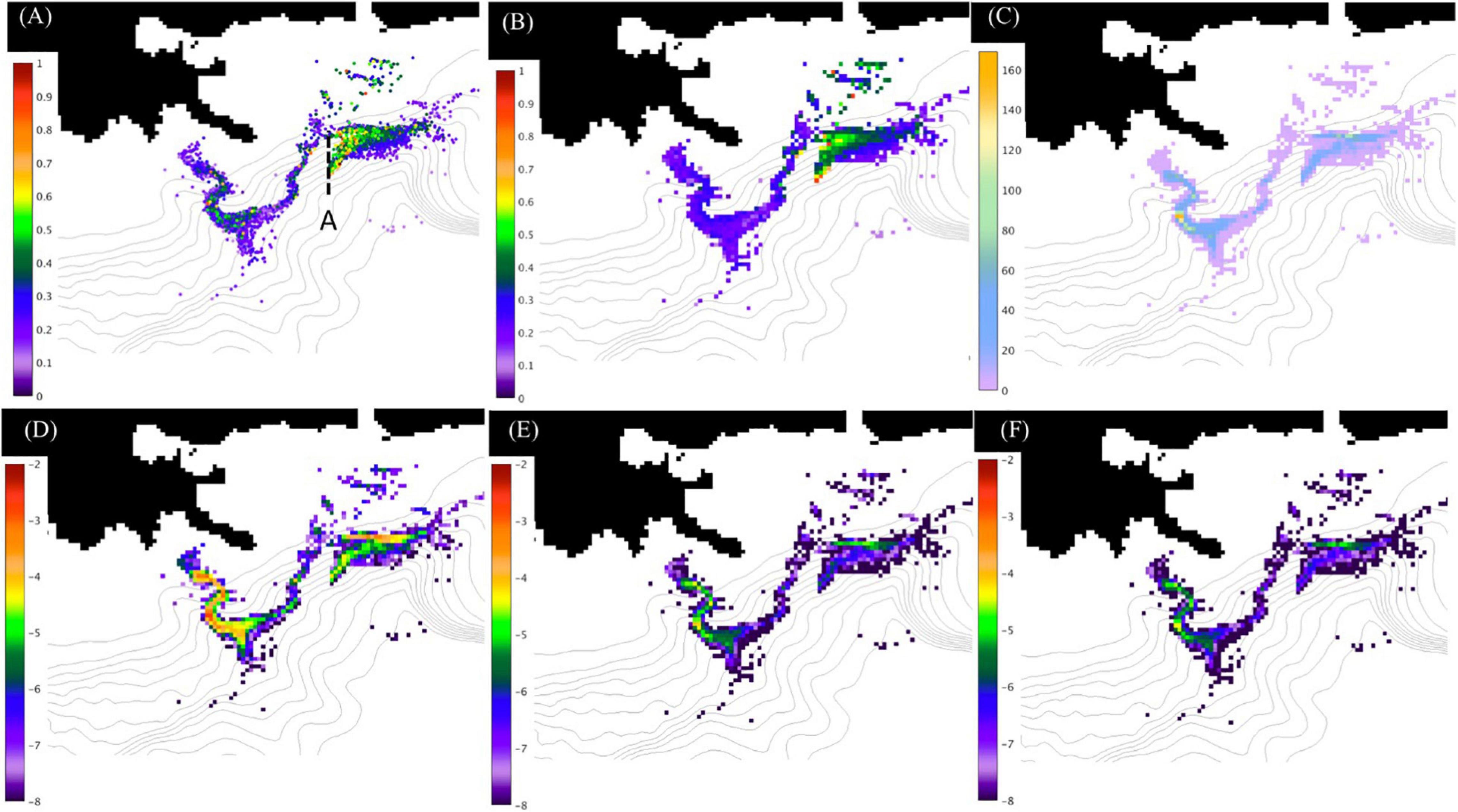
Figure 6. Demonstration of the LEM in a ROMS-OTWM test simulation in the model surface layer. (A) The dots indicate locations of individual Lagrangian floats. Colors show mean oil droplet size D_oil (μm). The dashed line A is the transect shown in Figure 7. (B–F) oil characteristics mapped onto an Eulerian model grid frame. (B) Mean oil droplet size in the grid cells $D_{oil}^{*}$ (μm). (C) Number of floats per grid cell. (D) Concentration of oil compound #1 (saturates), ${\tilde{C}}_{oil}^{*}(1)$ (natural log scale, kg m^–3). (E) Concentration of oil compound #2 (aromatics), ${\tilde{C}}_{oil}^{*}(2)$. (F) Concentration of oil compound #3 (resins and asphaltenes), ${\tilde{C}}_{oil}^{*}(3)$.

FIGURE 7

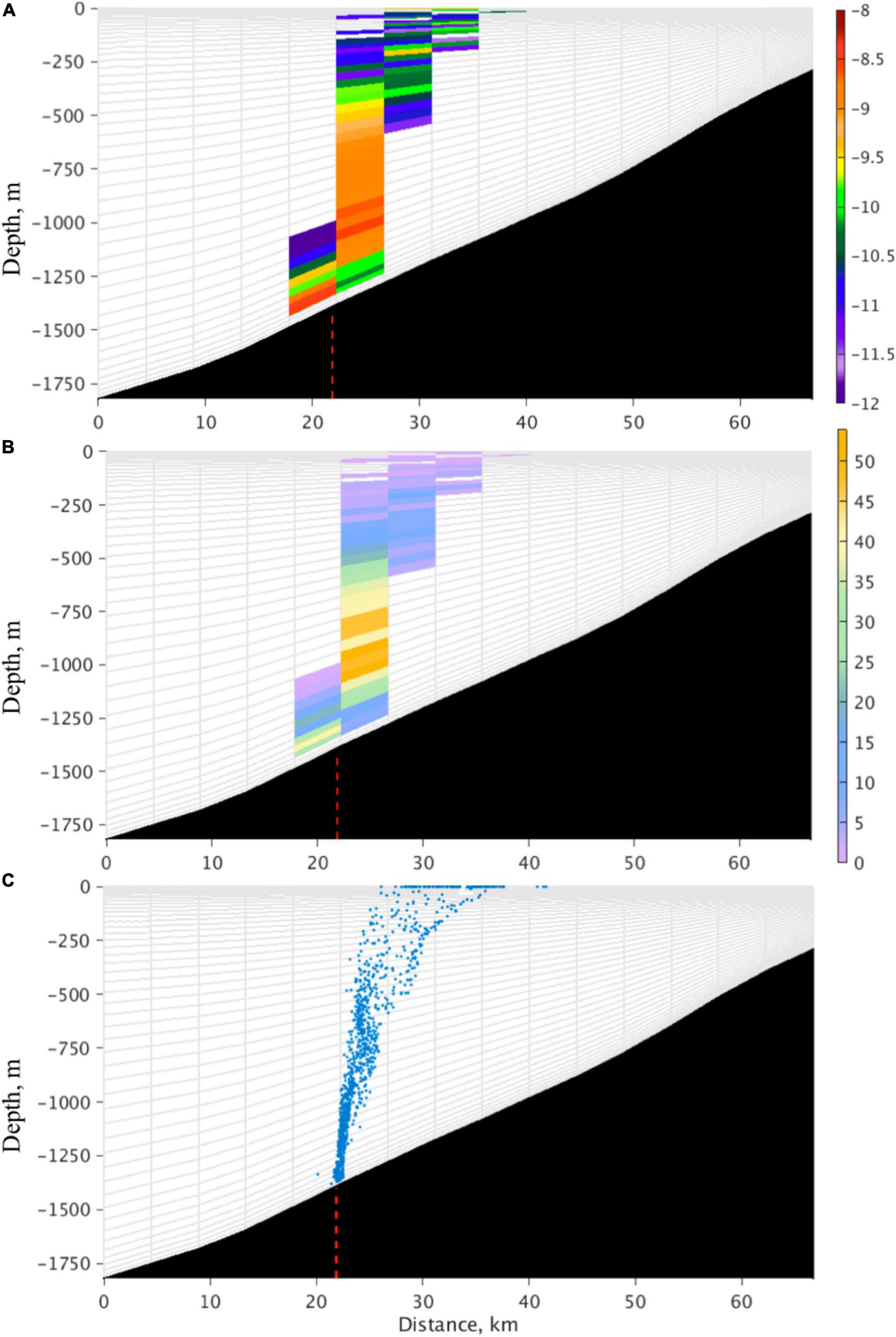
Figure 7. LEM of oil characteristics in the vertical. (A) Vertical distribution of oil concentration ($C_{oil}^{*}$, kg m^–3) on natural logarithmic scale along section A, shown in Figure 6A. The grid cells are indicated with gray lines. (B) Vertical distribution of Lagrangian float counts in the grid cells. The fields shown in (A,B) are obtained by LEM. (C) Lagrangian float positions. The red dashed line indicates location of the DWH and the approximate release location of the floats.

Eulerian-Lagrangian Mapping

Description of the Methodology

After the oil has been subject to biodegradation and sedimentation processes simulated in the biogeochemical and sediment-OPA modules, the modified oil fields (denoted in this section with index k+1) need to be mapped back to the Lagrangian framework and then updated by the OTWM. In the model, both the biogeochemical and sedimentation processes modify concentrations of the oil compounds but do not explicitly modify the size of oil particles. Therefore, the reverse mapping from the Eulerian to Lagrangian framework interprets changes in ${\tilde{C}}_{oil}^{*}$ in terms of oil droplet characteristics for each Lagrangian float. The assumption is that floats clustered in one grid cell undergo similar changes during biodegradation and sedimentation, and that changes of oil droplets are proportional to their size.

First, the new mass fraction of the oil compounds is updated at every grid cell (j) by calculating the reduction of concentration for the oil compounds (i)

$$r^{*}(\mathbf{j};i)=\frac{{\tilde{C}}_{oil}^{*(k+1)}(\mathbf{j};i)}{{\tilde{C}}_{oil}^{(k+1)}(\mathbf{j};i)}.(47)$$

Assuming similar reduction of the oil compounds across all particles in a given grid cell (j), the new mass fraction of the oil compounds in the Lagrangian elements within the grid cell is

$${\tilde{\mathrm{\omega }}}_{oil}^{(k+1)}(\mathbf{j};i)=\frac{r^{*}(\mathbf{j};i){\tilde{\mathrm{\omega }}}_{oil}^{(k)}(\mathbf{j};i)}{{\sum }_i^{N_{comp}}{r}^{*}(\mathbf{j};i){\tilde{\mathrm{\omega }}}_{oil}^{(k)}(\mathbf{j};i)}.(48)$$

Next, oil particle densities in the Lagrangian elements within the grid cell are updated

$${\mathrm{\rho }}_{oil}^{\left(k+1\right)}(l\in S(\mathbf{\text{j}}))={\left[\sum _{i=1}^{N_{comp}}\frac{{\tilde{\mathrm{\omega }}}_{oil}^{(k+1)}(\mathbf{j};i)}{{\tilde{\mathrm{\rho }}}_{oil}(i)}\right]}^{-1}.(49)$$

In order to update oil droplet size using Eq. 36, a new volume of oil particles ($v_{oil}^{(k+1)}$) is needed. This information is neither explicitly provided by the sediment nor by the biogeochemical modules. The following approach has been employed to derive $v_{oil}^{(k+1)}$. Let

$$v_{oil}^{(k+1)}=\mathrm{\alpha }{v}_{oil}^{(k)},(50)$$

where α is an unknown coefficient. Using the fact that mass of the oil is conserved in the Lagrangian and Eulerian spaces, the following is true

$$M_{oil}^{*\left(k+1\right)}\left(\mathbf{j}\right)=V_{grid}\left(\mathbf{j}\right)\sum _{i=1}^{N_{comp}}{C}_{oil}^{*\left(k+1\right)}(\mathbf{j};i)=$$

$$\sum _{l\in S(\mathbf{j})}{N}_{poil}^{(k+1)}(l)\cdot {\mathrm{\rho }}_{oil}^{(k+1)}(l)\cdot v_{oil}^{(k+1)}(l),(51)$$

where $N_{poil}^{(k+1)}$ is the number of oil particles in Lagrangian float l. In order to close the problem, it is assumed that the number of particles does not change during the biodegradation or formation of OPAs (only depletion of compounds occurs). Then, N_poil for a given Lagrangian float can be estimated from the initial fields as

$$N_{poil}=\frac{M_{oil}}{{\mathrm{\rho }}_{oil}{v}_{oil}}=\frac{{\vartheta }_{oil}}{v_{oil}},(52)$$

where M_oil is the mass of the oil in a Lagrangian float. Then, using Eqs 35 and 51, α can be found as (note $v_{oil}^{(k)}$ at time k in the equation)

$$\mathrm{\alpha }=\frac{M_{oil}^{*\left(k+1\right)}\left(\mathbf{j}\right)}{{\sum }_{l\in S(\mathbf{j})}{N}_{poil}(l)\cdot {\mathrm{\rho }}_{oil}^{(k+1)}(l)\cdot v_{oil}^{(k)}(l)}.(53)$$

Test Simulations With ELM

For testing the ELM, a more elaborate set of numerical experiments is prepared. One experiment is integrated with both the LEM and ELM implemented, but neither biogeochemical degradation nor sediment-OPA formation is activated. In the second experiment, the biogeochemical model is implemented and coupled with the ROMS-OTWM via LEM-ELM. In the first experiment, no changes in oil characteristics are expected to occur before the floats reach the surface. The purpose of these experiments is to validate that LEM-ELM does not change oil mass and oil characteristics in the first experiment and accurately maps changes in oil characteristics onto Lagrangian space in the second experiment.

Both experiments are integrated for 7 days. The changes in oil characteristics are analyzed over the ascent time of the floats, from the release of the floats near the bottom until they reach the surface where the oil is subject to surface evaporation. In the experiments, the median of the ascent time is 2.4 days and the 90^th percentile is 4.9 days.

In agreement with expectations, changes are not observed in the first experiment without subsurface oil degradation (the dashed lines in Figure 8). Thus, the LEM and ELM do not excite spurious changes in the oil characteristics. In the second experiment, subsurface biodegradation results in changes across the oil parameters that is also in agreement with expectations. For all floats, oil droplet density increases with time (Figure 8A), whereas both mass and size decrease as a result of oil consumption by microbes simulated in the biochemical model. In agreement with previous studies, lighter compounds of oil undergo biodegradation at a faster rate than the heavier oil. In the test simulation, both aromatics and saturates are consumed at a high rate, whereas the mass of the asphaltenes and resins barely changes (Figure 8E).

FIGURE 8

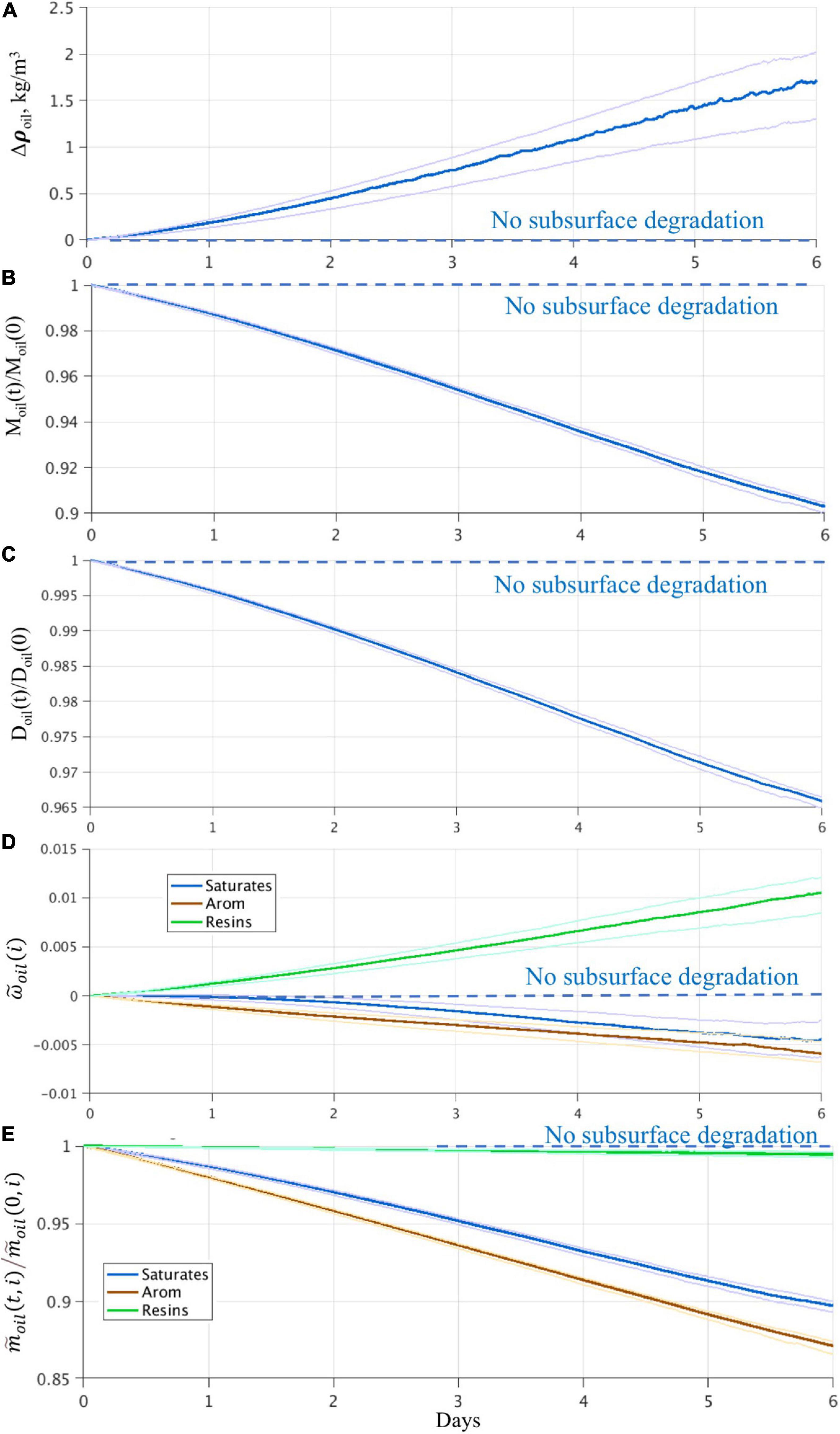
Figure 8. Statistics of changes in oil characteristics in the experiments using LEM and ELM with and without subsurface biodegradation from a coupled ROMS-OTWM-Biogeochemical model. (A) Change of oil droplet density (kg m^–3). (B) Reduction of the oil droplet mass relative to the original mass. (D) Reduction of the oil droplet size relative to the initial size. (C) Weight fraction of oil compounds. (E) Reduction of mass of oil compounds. The estimates are obtained from all floats over the first 6 days after the floats are released at the bottom and until they reach the surface. The solid line is the median, the lighter lines are the inter-quartile range. The horizontal dashed line indicates no change in oil characteristics in the experiment without subsurface degradation. The change in oil characteristics due to biodegradation demonstrates the impact of biogeochemical model coupling using LEM and ELM. The horizontal axis is subsurface time (days) of oil particles from the release until particles reach the surface.

Fully Coupled Test Simulation

To demonstrate the performance of the fully coupled CSOMIO model, a test simulation has been conducted. In this test simulation, oil floats are released near the bottom (∼1,400 m) at five locations around the Macondo wellhead (the locations are within ∼100 m) at a frequency of one float every 2.7 min. A constant oil flow rate of 3,000 m³ day^–1 is prescribed, thus one float represents 1.1 m³ of oil. The total number of floats is 80,000. All other forcing fields and characteristics are identical to the test simulations presented earlier in the paper. The model is integrated for 30 days with the fully coupled ROMS-OTWM-OPAMOD-biogeochemical. It should be mentioned that the test simulation was not designed to hindcast the DWH event. Such an effort would require additional tuning of free parameters in the model (Morey et al., 2018.). The purpose of this test simulation was merely to demonstrate the performance of the CSOMIO modeling system with all components coupled.

In the upper ocean, we see the oil has spread approximately 400 km around the release location during the simulation (Figure 9) and most of the oil has drifted toward the coast. There is a substantial amount of oil in the subsurface layers, as well (Figure 9A). Mass density of the oil compounds differ because of different biodegradation and weathering rates, as well as different initial distributions of the oil compounds (Figure 5A). At the surface, saturates has the fastest depletion rate due to evaporation, whereas resins and asphaltenes have the slowest evaporation. Therefore, mass density of the heavy oil compounds (Figure 9D) is comparable to mass density of the other two compounds (Figures 9B,C) and it is even higher in the western part of the simulated spill where the oil has been subject to evaporation over a longer period of time.

FIGURE 9

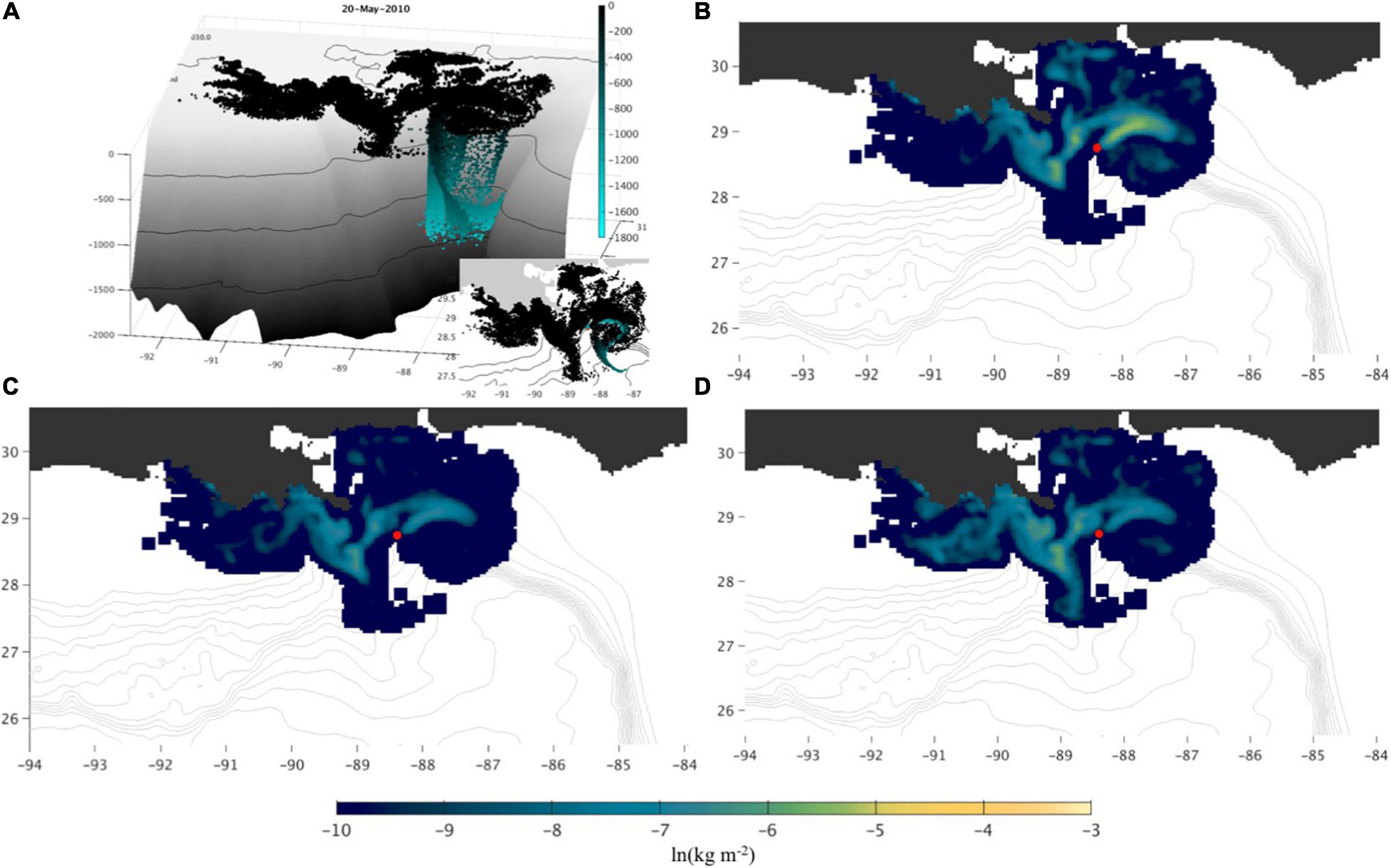
Figure 9. Simulated oil from the test experiment with the fully coupled ROMS-OTWM-OPAMOD-Biogeochemical model after 30 days of simulation. (A) Three-dimensional distribution of Lagrangian floats representing clusters of oil particles. The red dot indicates release location at the bottom. Colors designate particles’ depth in the water column. (B–D) Mass density (kg m^–2) of the oil compounds (saturates, aromatics, resins and asphaltenes, respectively) in the upper 50 m. Mass density is on the natural logarithmic scale.

During the oil spill, the most rapid increase is simulated for bacteria 2 (Figures 10A,B) feeding on saturates. It takes time for a bacterial community to respond, thus higher concentrations of bacteria 2 and bacteria 3 are observed farther away from the spill location in the oil that remains the longest in the subsurface layers (Figures 10A,C). Bacteria 4, feeding on the heavy oil compounds, has the slowest increase rate (Figures 10E,F). Its concentration has barely increased over the simulation time and is similar to the background concentration. In the vertical sections, elevated concentrations of the oil-degrading bacteria highlight the track of the oil plume in the subsurface layers (Figures 10B,D,F).

FIGURE 10

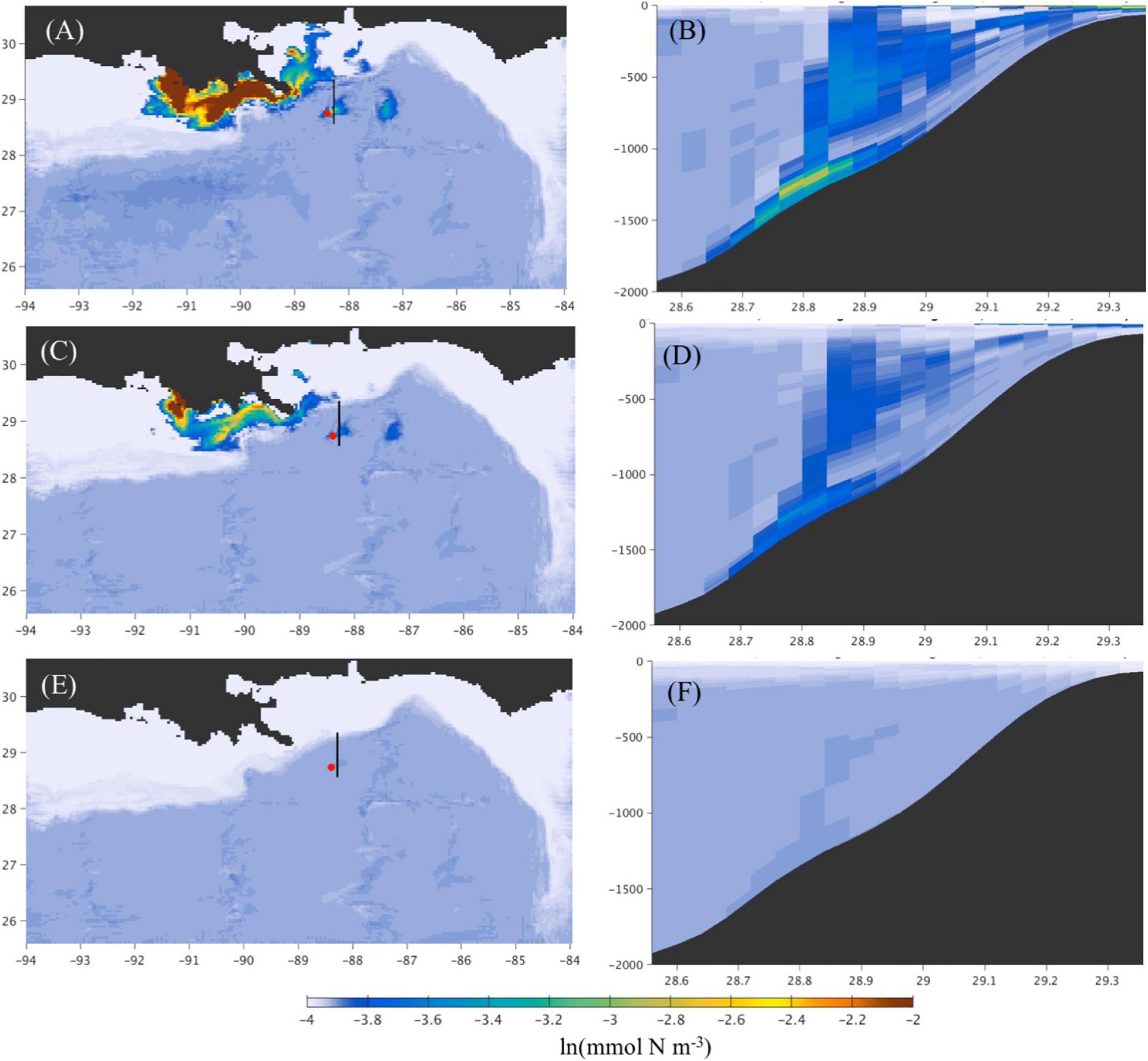
Figure 10. Dissolved bacteria concentration (mmol N m^–3) from the test experiment with the fully coupled ROMS-OTWM-OPAMOD-Bgeochemical model after 30 days of simulation. (A,C,E) Spatial distribution of bacteria 2 (saturates), 3 (aromatics), and 4 (heavy oil), respectively, in the near-bottom layer (5th layer from the bottom). The red dot is the release location of the Lagrangian floats. (B,D,F) are the vertical distribution of bacteria 2, 3, 4 concentration along the section indicated with the black line in the left figures. Plots are in the natural logarithmic scale.

Formation of the sediment OPAs is mainly limited to the deep region within 100–150 km of the release location (Figure 11) because of the high concentration of oil droplets in the near-bottom layer over this area. Spatial distribution of the OPAs is inhomogeneous and extends in the eastern direction due to the mean near-bottom flow over the simulated time period. Sediment OPA1 has higher concentration and is more widely spread compared to the other OPA classes. This is consistent with results from sensitivity tests in a one-dimensional (vertical) model (Cui et al., 2020), that is, with intermediate fractal dimensions (2.39 in this study), the diameter of the dominant OPA classes fall in the range of 180–360 μm (the diameter of OPA1 here is 256 μm). Because the settling velocity of OPA types 2–4 are greater than that of the OPA1 (see Table 3), they deposit and settle into slower moving water more quickly than OPA1. This results in OPA1 being more widely dispersed than the more slowly settling classes of OPA.

FIGURE 11

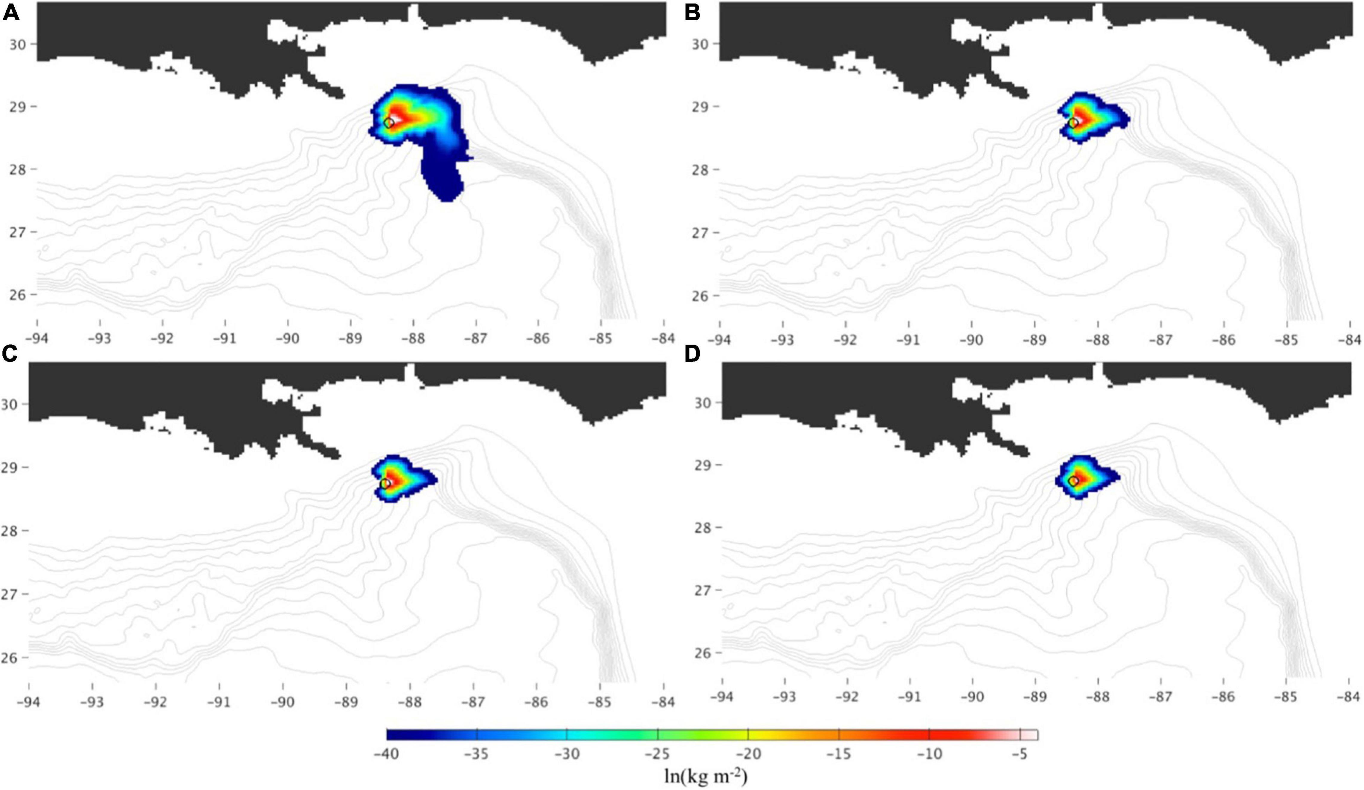
Figure 11. Sediment OPAs (kg m^–2) from the test experiment with the fully coupled ROMS-OTWM-OPAMOD-Biogeochemical model after 30 days of simulation. The OPAs are depth-integrated. Sediment OPAs 1–4 are shown in (A–D), respectively.

The results of this test simulation demonstrate the capabilities of the CSOMIO modeling system in a coupled configuration. Model components of oil, sediment, and biology interact and show the generally expected responses.

Summary and Closing Remarks

The newly developed CSOMIO coupled modeling system presented here is designed to simulate three-dimensional movement of oil in the ocean and compositional changes of oil (weathering) in the water column and at the surface, with explicitly modeled interactions with evolving sediment and biological components as opposed to prescribed parameterizations. The system is based on COAWST (Warner et al., 2010) and includes oil transport and weathering (OTWM), OPAMOD, and biogeochemical modules that can be integrated in a coupled or uncoupled configuration. For coupling OTWM with OPAMOD and biogeochemical modules, a two-way Lagrangian-Eulerian mapping has been developed and implemented for mass-conservative two-way exchange of the information between the Lagrangian and Eulerian frameworks. The system can be integrated in online or offline configuration. The latter drastically reduces computational time and is particularly useful for performing multiple simulations with a fully coupled CSOMIO model.

In the simulations described in this paper, the chemical composition of oil is described in terms of three chemical compounds (saturates, aromatics, resins and asphaltenes or SAR+A). This allows for tracking changes of individual oil compounds. This is important for realistic representation of oil weathering because different oil compounds have dramatically different degradation rates. Moreover, simulations of biogeochemical processes and OPA formation rely on information about individual oil compounds in the ocean.

Numerous test runs have been conducted to assess performance of the individual components of the modeling system, as well as the whole system both in online and offline configurations. Results of these simulations (some of which have been presented here) demonstrate realistic movement of oil in the water column and at the surface, as well as its interaction with the sedimentation and biochemical constituents. The modeling code can be configured for simulation of particular spill events (see Morey et al., 2018). The following parameters need to be validated and adjusted for an individual oil spill event.

(1) Oil density parameters. Oil chemical composition differs depending on its origin. The difference is due to varying proportions of the compounds in different type of oils. Hence, densities of the oil compounds need to be adjusted for any particular oil. Weight fractions of the oil compounds are specified in the code (hard coded) and can be easily changed. The code can also be modified to include more than three (currently) oil compounds.

(2) Parameters controlling the ascent rate of oil particles in the float input file (${\overline{D}}_{oil}$ and algorithm for computing oil particle vertical velocity).

(3) Surface oil drift parameters (C_w). Wind drag coefficient should be tuned for ocean surface currents depending on how accurately these currents represent wind-driven surface flow.

(4) Characteristics and representation of the oil spill (flow rate, release locations and frequency of Lagrangian floats).

The existing CSOMIO code is a ready-to-use tool, however, the model would benefit from future applications to realistic simulations during which the code could undergo further testing and improvements. The code is publicly available through the Gulf of Mexico Research Initiative Information and Data Cooperative (GRIIDC) (Dukhovskoy et al., 2020). The version of the code available through the GRIIDC does not currently have the offline capability.

Several additions to the model could be made to improve the performance of the CSOMIO model:

(1) Optimization of the Lagrangian float code to better perform on parallel multiprocessor systems. The performance of the this module degrades as the number of floats increases;

(2) Implementation of variable number of oil compounds (which is currently set to three);

(3) Addition of a near-field module to simulate initial size of droplets distribution near the oil release;

(4) Representation of other weathering processes (photo oxidation, emulsification, wave mixing);

(5) Addition of wave effect to the surface oil drift;

(6) Addition of droplet size dependent hydrocarbon uptake, because the surface area is thought to determine uptake rather than concentrations.

(7) Addition of biological aggregates comprising oil and sediment particles (Alldredge and Silver, 1988; Passow et al., 2012; Daly et al., 2016).

(8) Development of a rapid deployment tool suite that allows for model reconfiguration for other regions without extensive and time-consuming preparation of forcing fields and initial conditions.

Data Availability Statement

The datasets presented in this study can be found in online repositories. The names of the repository/repositories and accession number(s) can be found below: https://data.gulfresearchinitiative.org. The dataset page is https://data.gulfresearchinitiative.org/data/R6.x803.000:0017. The dataset doi: 10.7266/JYQJVN6N

Author Contributions

DD developed OWTM, ELM, LEM codes and wrote the first draft of the manuscript. CH, LC, AM, and T-JH developed and tested OPAMOD. VC, JW, MS, and XC developed and tested the biochemical model. DD, KT, XC, and SM implemented and tested the offline algorithm in CSOMIO. CH, LC, VC, and JW wrote sections of the manuscript. All authors contributed to conception and design of the study. All authors contributed to writing, read, and approved the submitted version.

Funding

This research was made possible by the grant from the Gulf of Mexico Research Initiative. This manuscript is Contribution No. 3992 of the Virginia Institute of Marine Science, William and Mary.

Conflict of Interest

AM was employed by company HR Wallingford Ltd., United Kingdom.

The remaining authors declare that the research was conducted in the absence of any commercial or financial relationships that could be construed as a potential conflict of interest.

Acknowledgments

We thank Tracy Ippolito (FSU) for proof-reading the manuscript and for the administrative support during the CSOMIO project.

References

Abascal, A. J., Castanedo, S., Mendez, F. J., Medina, R., and Losada, I. J. (2009). Calibration of a Lagrangian transport model using drifting buoys deployed during the Prestige oil spill. J. Coastal Res. 25, 80–90. doi: 10.2112/07-0849.1

CrossRef Full Text | Google Scholar

Alldredge, A. L., and Silver, M. W. (1988). Characteristics, dynamics and significance of marine snow. Prog. Oceanogr. 20, 41–82. doi: 10.1016/0079-6611(88)90053-5

CrossRef Full Text | Google Scholar

American Society of Civil Engineers Committee on Modeling Oil Spills (1996). State-of the-art review of modeling transport and fate of oil spills. J. Hydraul. Eng. 122, 594–609.

Google Scholar

Bahadori, A., Mahmoudi, M., and Nouri, A. (2015). Prediction of heavy-oil viscosities with a simple correlation approach. Oil Gas Facil. 4, 66–72. doi: 10.2118/157360-PA

PubMed Abstract | CrossRef Full Text | Google Scholar

Bandara, U. C., Yapa, P. D., and Xie, H. (2011). Fate and transport of oil in sediment laden marine waters. J. Hydro Environ. Res. 5, 145–156. doi: 10.1016/j.jher.2011.03.002

CrossRef Full Text | Google Scholar

Bracco, A., Paris, C. B., Esbaugh, A. J., Frasier, K., Joye, S. B., Liu, G., et al. (2020). Transport, fate and impacts of the deep plume of petroleum hydrocarbons formed during the Macondo blowout. Front. Mar. Sci. 7:764. doi: 10.3389/fmars.2020.542147

CrossRef Full Text | Google Scholar

Camilli, R., Reddy, C. M., Yoerger, D. R., Van Mooy, B. A. S., Jakuba, M. V., Kinsey, J. C., et al. (2010). Tracking hydrocarbon plume transport and biodegradation at Deepwater Horizon. Science 330, 201–204. doi: 10.1126/science.1195223

PubMed Abstract | CrossRef Full Text | Google Scholar

Chen, F., and Yapa, P. D. (2003). A model for simulating deep water oil and gas blowouts – Part II: comparison of numerical simulations with Deepspill field experiments. J. Hydr. Res. 41, 353–365. doi: 10.1080/00221680309499981

CrossRef Full Text | Google Scholar

Coles, V. J., Stukel, M. R., Brooks, M. T., Burd, A., Crump, B. C., Moran, M. A., et al. (2017). Ocean biogeochemistry modeled with emergent trait-based genomics. Science 358, 1149–1154. doi: 10.1126/science.aan5712

PubMed Abstract | CrossRef Full Text | Google Scholar

Cui, L., Harris, C. K., and Tarpley, D. R. N. (2020). Formation of oil-particle-aggregates (OPAs): numerical model formulation and calibration. Front. Mar. Sci.

Google Scholar

Daly, K. L., Passow, U., Chanton, J., and Hollander, D. (2016). Assessing the impacts of oil-associated marine snow formation and sedimentation during and after the Deepwater Horizon oil spill. Anthropocene 13, 18–33. doi: 10.1016/j.ancene.2016.01.006

CrossRef Full Text | Google Scholar

Davis, C. S., and Loomis, N. C. (2014). Deepwater Horizon Oil Spill (DWHOS) Water Column Technical Working Group, Image Data Processing Plan: Holocam Description of Data Processing Methods Used to Determine Oil Droplet Size Distributions from in situ Holographic Imaging During June 2010 on Cruise M/V Jack Fitz 3. Woods Hole, MA: Woods Hole Oceanographic Institution and MIT.

Google Scholar

Diercks, A. R., Highsmith, R. C., Asper, V. L., Joung, D., Zhou, Z., Guo, L., et al. (2010). Characterization of subsurface polycyclic aromatic hydrocarbons at the deepwater horizon site. Geophys. Res. Lett. 37, 1–6. doi: 10.1029/2010GL045046

CrossRef Full Text | Google Scholar

Dukhovskoy, D., Harris, C., Cui, L., Coles, V., Wang, J., Chen, X., et al. (2020). CSOMIO Open Source Model System. Tallahassee, FL: GRIDC Gulf of Mexico Research Initiative.

Google Scholar

Dyer, K. R., and Manning, A. J. (1999). Observation of the size, settling velocity and effective density of flocs, and their fractal dimensions. J. Sea Res. 41, 87–95. doi: 10.1016/s1385-1101(98)00036-7

CrossRef Full Text | Google Scholar

Fennel, K., Wilkin, J., Levin, J., Moisan, J., O’Reilly, J., and Haidvogel, D. (2006). Nitrogen cycling in the middle atlantic bight: results from a three-dimensional model and implications for the North Atlantic nitrogen budget. Glob. Biogeochem. Cycles 20, 1–14. doi: 10.1029/2005GB002456

CrossRef Full Text | Google Scholar

Fingas, M. (1995). A literature review of the physics and predictive modelling of oil spill evaporation. J. Hazard. Mater. 42, 157–175. doi: 10.1016/0304-3894(95)00013-k

CrossRef Full Text | Google Scholar

Fingas, M. (1996). The evaporation of oil spills: prediction of equations using distillation data. Spill Sci. Technol. Bull. 3, 191–192. doi: 10.1016/s1353-2561(97)00009-1

CrossRef Full Text | Google Scholar

Fingas, M. (2012). Studies on the evaporation regulation mechanisms of crude oil and petroleum products. Adv. Chem. Eng. Sci. 2, 246–256. doi: 10.4236/aces.2012.22029

CrossRef Full Text | Google Scholar

Fingas, M. (2015b). “Evaporation modeling,” in Handbook of Oil Spill Science and Technology, ed. M. Fingas (Hoboken, NJ: John Wiley & Sons), 201–242.

Google Scholar

Fingas, M. (2015a). “Introduction to oil chemistry and properties,” in Handbook of Oil Spill Science and Technology, ed. M. Fingas (Hoboken, NJ: John Wiley & Sons), 51–77.

Google Scholar

French-McCay, D., Li, Z., Horn, M., Crowley, D., Spaulding, M. L., Mendelson, D., et al. (2016). “Modeling oil fate and subsurface exposure concentrations from the deepwater horizon oil spill,” in Proceedings of the Thrity-ninth AMOP Technical Seminar, (Ottawa, ON: Environment and Climate Change Canada), 115–150.

Google Scholar

French-McCay, D., and Payne, J. R. (2001). “Model of oil fate and water concentrations with and without application of dispersants,” in Proceedings of the 24th Arctic and Marine Oilspill (AMOP) Technical Seminar, Edmonton, Alberta, Canada, June 12-14, 2001, (Vancouver, BC: Environment Canada), 611–645.

Google Scholar

Garcia-Martinez, R., and Flores-Tovar, H. (1999). Computer modeling of oil spill trajectories with a high accuracy method. Spill Sci. Technol. B. 5, 323–333. doi: 10.1016/s1353-2561(99)00077-8

CrossRef Full Text | Google Scholar

Harris, C. K., Syvitski, J., Arango, H. G., Meiburg, E. H., Cohen, S., Jenkins, C. J., et al. (2020). Data-driven, multi-model workflow suggests strong influence from hurricanes on the generation of turbidity currents in the Gulf of Mexico. J. Mar. Sci. Eng. 8:28. doi: 10.3390/jmse8080586

CrossRef Full Text | Google Scholar

Hiester, H.R., Morey, S. L., Dukhovskoy, D., Chassignet, E. P., Kourafalou, V. H., and Hu, C. (2016). A topological approach for quantitative comparisons of ocean model fields to satellite ocean color data. Methods Oceanogr.. 17, 232–250.

Google Scholar

Hope, J. A., Malarkey, J., Baas, J. H., Peakall, J., Parsons, D. R., Manning, A. J., et al. (2020). Interactions between sediment microbial ecology and physical dynamics drive heterogeneity in contextually similar depositional systems. Limnol. Oceanogr. 65, 2403–2419. doi: 10.1002/lno.11461

CrossRef Full Text | Google Scholar

Isobe, A., Kako, S., Chang, P., and Matsuno, T. (2009). Two-way particle-tracking model for specifying sources of drifting objects: application to the East China sea shelf. J. Atmos. Oceanic Technol. 26, 1672–1682. doi: 10.1175/2009JTECHO643.1

CrossRef Full Text | Google Scholar

Klein, G. C., Angstrom, A., Rodgers, R. P., and Marshall, A. G. (2006). Use of Saturates/Aromatics/Resins/Asphaltenes (SARA) fractionation to determine matrix effects in crude oil analysis by electrospray ionization fourier transform ion cyclotron resonance mass spectrometry. Energy Fuels 20, 668–672. doi: 10.1021/ef050353p

CrossRef Full Text | Google Scholar

Kranenburg, C. (1994). The fractal structure of cohesive sediment aggregates. Estuar. Coast. Shelf Sci. 39, 451–460. doi: 10.1006/ecss.1994.1075

CrossRef Full Text | Google Scholar

Lardner, R., and Zodiatis, G. (2017). Modelling oil plumes from subsurface spills. Mar. Pollut. Bull. Bull. 124, 94–101. doi: 10.1016/j.marpolbul.2017.07.018

PubMed Abstract | CrossRef Full Text | Google Scholar

Laurent, A., Fennel, K., Hu, J., and Hetland, R. (2012). Simulating the effects of phosphorus limitation in the Mississippi and atchafalaya river plumes. Biogeosciences 9, 4707–4723. doi: 10.5194/bg-9-4707-2012

CrossRef Full Text | Google Scholar

Lehr, W., Jones, R., Evans, M., Simecek-Beatty, D., and Overstreet, R. (2002). Revisions of the ADIOS oil spill model. Environ. Modell. Softw. 17, 191–199.

Google Scholar

Li, Z., Lee, K., King, T., Boufadel, M. C., and Venosa, A. D. (2008). Assessment of chemical dispersant effectiveness in a wave tank under regular non-braking and wave breaking wave conditions. Mar. Pollut. Bull. 56, 903–912. doi: 10.1016/j.marpolbul.2008.01.031

PubMed Abstract | CrossRef Full Text | Google Scholar

Lindo-Atichati, D., Paris, C. B., Le Hénaff, M., Schedler, M., Valladares Juárez, A. G., and Müller, A. (2016). Simulating the effects of droplet size, high-pressure biodegradation, and variable flow rate on the subsea evolution of deep plumes from the Macondo blowout. Deep Sea Res. II Top. Stud. Oceanogr. 129, 301–310. doi: 10.1016/j.dsr2.2014.01.011

CrossRef Full Text | Google Scholar

Lonin, S. A. (1999). Lagrangian model for oil spill diffusion at sea. Spill Sci. Technol. B 5, 331–336. doi: 10.1016/s1353-2561(99)00078-x

CrossRef Full Text | Google Scholar

Lubchenco, J., McNutt, M., Lehr, B., Sogg, M., Miller, M., Hammond, S., et al. (2010). Deepwater Horizon/BP Oil Budget: What Happened to the Oil? National Oceanic and Atmospheric Administration Report. Silver Spring, MD: National Oceanic and Atmospheric Administration.

Google Scholar

Lubchenco, J., McNutt, M. K., Dreyfus, G., Murawski, S. A., Kennedy, D. M., Anastas, P. T., et al. (2012). Science in support of the Deepwater Horizon response. Proc. Nat. Acad. Sci. U.S.A. 109, 20212–20221. doi: 10.1073/pnas.1204729109

PubMed Abstract | CrossRef Full Text | Google Scholar

MacDonald, I. R., Dukhovskoy, D., Bourassa, M., Morey, S., Garcia-Pindea, O., Daneshgar, A., et al. (2016). Remote Sensing Assessment of Surface Oil Transport and Fate during Spills in the Gulf of Mexico. New Orleans, LA: U.S. Department of the Interior, 115.

Google Scholar

Manning, A. J., Whitehouse, R. J. S., and Uncles, R. J. (2017). “Suspended particulate matter: the measurements of flocs,” in ECSA Practical Handbooks on Survey and Analysis Methods: Estuarine and Coastal Hydrography and Sedimentology, Chapter 8, eds R. J. Uncles and S. Mitchell (Cambridge: Cambridge University Press), 211–260. doi: 10.1017/9781139644426

CrossRef Full Text | Google Scholar

Mason, O. U., Hazen, T. C., Borglin, S., Chain, P. S. G., Dubinsky, E. A., Fortney, J. L., et al. (2012). Metagenome, metatranscriptome and single-cell sequencing reveal microbial response to Deepwater Horizon oil spill. ISME J. 6, 1715–1727. doi: 10.1038/ismej.2012.59

PubMed Abstract | CrossRef Full Text | Google Scholar

Mehta, A. J., Manning, A. J., and Khare, Y. P. (2014). A Note on the Krone deposition equation and significance of floc aggregation. Mar. Geol. 354, 34–39. doi: 10.1016/j.margeo.2014.04.002

CrossRef Full Text | Google Scholar

Melvin, A. T., Thibodeaux, L. J., Parsons, A. R., Overton, E., Valsaraj, K. T., and Nandakumar, K. (2016). Oil-material fractionation in Gulf deep water horizontal intrusion layer: Field data analysis with chemodynamic fate model for Macondo 252 oil spill. Mar. Pollut. Bull. 105, 110–119. doi: 10.1016/j.marpolbul.2016.02.043

PubMed Abstract | CrossRef Full Text | Google Scholar

Molski, A. (1989). On the collision efficiency approach to flocculation. Coll. Polym. Sci. 267, 371–375. doi: 10.1007/BF01413632

CrossRef Full Text | Google Scholar

Morey, S., Wienders, N., Dukhovskoy, D. S., and Bourassa, M. A. (2018). Measurement characteristics of near-surface currents from ultra-thin drifters, drogued drifters, and HF radar. Rem. Sens. 10:1633. doi: 10.3390/rs10101633

CrossRef Full Text | Google Scholar

North, E. W., Adams, E. E., Thessen, A. W., Schalg, Z., He, R., Socolofsky, S. A., et al. (2015). The influence of droplet size and biodegradation on the transport of subsurface oil droplets during theDeepwater Horizon spill: a model sensitivity study. Environ. Res. Lett. 10:024016. doi: 10.1088/1748-9326/10/2/024016

CrossRef Full Text | Google Scholar

Özgökmen, T. M., Chassignet, E. P., Dawson, C. N., Dukhovskoy, D., Jacobs, G., Ledwell, J., et al. (2016). Over what area did the oil and gas spread during the 2010 Deepwater Horizon oil spill? Oceanography 29, 96–107.

Google Scholar

Paris, C. B., Le Hénaff, M., Aman, Z. M., Subramaniam, A., Helgers, J., Wang, D. P., et al. (2012). Evolution of the Macondo well blowout: simulating the effects of the circulation and synthetic dispersants on the subsea oil transport. Environ. Sci. Technol. 46, 13293–13302. doi: 10.1021/es303197h

PubMed Abstract | CrossRef Full Text | Google Scholar

Parsons, D. R., Schindler, R. J., Hope, J. A., Malarkey, J., Baas, J. H., Peakall, J., et al. (2016). The role of biophysical cohesion on subaqueous bed form size. Geophys. Res. Lett. 43, 1566–1573. doi: 10.1002/2016GL067667

PubMed Abstract | CrossRef Full Text | Google Scholar

Passow, U., Ziervogel, K., Asper, V., and Diercks, A. (2012). Marine snow formation in the aftermath of the Deepwater Horizon oil spill in the Gulf of Mexico. Environ. Res. Lett. 7:035301.

Google Scholar

Perlin, N., Berenshtein, I., Vaz, A. C., Faillettaz, R., Schwing, P. T., Romero, P. T., et al. (2020). “Far-field modeling of deep-sea blowout: sensitivity studies of initial conditions, biodegradation, sedimentation and SSDI on surface slicks and oil plume concentrations,” in Deep Oil Spills: Facts, Fate, Effects, eds S. A. Murawski, C. Ainsworth, S. Gilbert, D. Hollander, C. B. Paris, M. Schlüter, et al. (Cham: Springer).

Google Scholar

Peters, F., and Arabali, D. (2013). Interfacial tension between oil and water measured with a modified contour method. Coll. Surf. A Physiochem. Eng. Aspects 426, 1–5.

Google Scholar

Reddy, C. M., Arey, J. S., Seewald, J. S., Sylva, S. P., Lemkau, K. L., Nelson, R. K., et al. (2012). Composition and fate of gas and oil released to the water column during the Deepwater Horizon oil spill. Proc. Natl. Acad. Sci. U.S.A. 109, 20229–20234. doi: 10.1073/pnas.1101242108

PubMed Abstract | CrossRef Full Text | Google Scholar

Reed, D. C., Algar, C. K., Huber, J. A., and Dick, G. J. (2014). Gene-centric approach to integrating environmental genomics and biogeochemical models. Proc. Natl. Acad. Sci. U.S.A. 111, 1879–1884. doi: 10.1073/pnas.1313713111

PubMed Abstract | CrossRef Full Text | Google Scholar

Reed, M., Johansen, O., Brandvik, P. J., Daling, P., Lewis, A., Fiocco, R., et al. (1999). Oil spill modeling towards the close of the 20th century: overview of the state of the art. Spill Sci. Technol. Bull. 5, 3–16. doi: 10.1016/s1353-2561(98)00029-2

CrossRef Full Text | Google Scholar

Reed, M., Turner, C., and Odulo, A. (1994). The role of wind and emulsification in modelling oil spill and surface drifter trajectories. Spill SciTechnol. B. 1, 143–157.

Google Scholar

Roden, E. E., and Jin, Q. (2011). Thermodynamics of microbial growth coupled to metabolism of glucose, ethanol, short-chain organic acids, and hydrogen. Appl. Environ. Microbiol. 77, 1907–1909. doi: 10.1128/AEM.02425-10

PubMed Abstract | CrossRef Full Text | Google Scholar

Roels, J. A. (1981). The application of macroscopic principles to microbial metabolism. Ann. N. Y. Acad. Sci. 369, 113–134. doi: 10.1111/j.1749-6632.1981.tb14182.x

CrossRef Full Text | Google Scholar

Sanchez-Minero, F., Sanchez-Reyna, G., Ancheyta, J., and Marroquin, G. (2014). Comparison of correlations based on API gravity for predicting viscosity of crude oils. Fuel 138, 193–199. doi: 10.1016/j.fuel.2014.08.022

CrossRef Full Text | Google Scholar

Saha, S., Moorthi, S., H?L Pan, X. W., Wang, J., Nadiga, S., Tripp, P., et al. (2010). The NCEP climate forecast system reanalysis. Bull. Am. Meteorol. Soc. 91, 1015–1058. doi: 10.1175/2010BAMS3001.1

CrossRef Full Text | Google Scholar

Samuels, W. B., Huang, N. E., and Amstutz, D. E. (1982). An oilspill trajectory analysis model with a variable wind deflection angle. Ocean Eng. 9, 347–360.

Google Scholar

Sharqay, M. H., Lienhard, J. H., and Zubair, S. M. (2010). Thermophysical properties of seawater: a review of existing correlations and data. Desal. Water Treat. 16, 354–380. doi: 10.5004/dwt.2010.1079

PubMed Abstract | CrossRef Full Text | Google Scholar

Sherwood, C. R., Aretxabaleta, A. L., Harris, C. K., Rinehimer, J. P., Verney, R., and Ferré, B. (2018). Cohesive and mixed sediment in the Regional Ocean Modeling System (ROMS v3.6) implemented in the Coupled Ocean–Atmosphere–Wave–sediment transport modeling system (COAWST r1234). Geosci. Model Dev. 11, 1849–1871. doi: 10.5194/gmd-11-1849-2018

CrossRef Full Text | Google Scholar

Socolofsky, S. A., Adams, E. E., Paris, C. B., and Yang, D. (2016). How do oil, gas, and water interact near a subsea blowout? Oceanography 29, 64–75. doi: 10.5670/oceanog.2016.63

CrossRef Full Text | Google Scholar

Socolofsky, S. A., Adams, E. E., and Sherwood, C. R. (2011). Formation dynamics of subsurface hydrocarbon intrusions following the Deepwater Horizon blowout. Geophys. Res. Lett. 38:L09602. doi: 10.1029/2011GL047174

CrossRef Full Text | Google Scholar

Soulsby, R. L., Manning, A. J., Spearman, J., and Whitehouse, R. J. S. (2013). Settling velocity and mass settling flux of flocculated estuarine sediments. Mar. Geol. 339, 1–12. doi: 10.1016/j.margeo.2013.04.006

CrossRef Full Text | Google Scholar

Spaulding, M. S., Li, Z., Mendelsohn, D., Crowley, D., French-McCay, D., and Bird, A. (2017). Application of an integrated blowout model system, OILMAP DEEP, to the deepwater horizon (DWH) spill. Mar. Pollut. Bull. 120, 37–50. doi: 10.1016/j.marpolbul.2017.04.043

PubMed Abstract | CrossRef Full Text | Google Scholar

Speight, J. G. (2007). The Chemistry and Technology of Petroleum, 4th Edn. Boca Raton, FL: CRC Press, 980.

Google Scholar

Stiver, W., and Mackay, D. (1984). Evaporation rate of spills of hydrocarbons and petroleum mixtures. Environ. Sci. Technol. 11, 834–840. doi: 10.1021/es00129a006

PubMed Abstract | CrossRef Full Text | Google Scholar

Thyng, K. M., Kobashi, D., Ruiz-Xomchuk, V., Qu, L., Chen, X., and Hetland, R. D. (2021). Performance of offline passive tracer advection in the Regional Ocean Modeling System (ROMS; v3.6, revision 904). Geosci. Model Dev. 14, 391–407. doi: 10.5194/gmd-14-391-2021

CrossRef Full Text | Google Scholar

U.S. Senate Committee on Environment and Public Works (2010). Timeline of the Gulf Coast Oil Spill and Emergencey Response. Available online at: https://www.epw.senate.gov/public/index.cfm/2010/5/post-8408bd41-802a-23ad-4464-ad127e495a41 (accessed May 7, 2010).

Google Scholar

Valentine, D. L., Mezić, I., Maćešić, S., Črnjarić-Žic, N., Ivić, S., Hogan, P. J., et al. (2012). Dynamic autoinoculation and the microbial ecology of a deep water hydrocarbon irruption. Proc. Natl. Acad. Sci. U.S.A. 109, 20286–20291. doi: 10.1073/pnas.1108820109

PubMed Abstract | CrossRef Full Text | Google Scholar

van der Mheen, M., Charitha, P., Simone, C., and Moritz, W. (2020). Depth-dependent correction for wind-driven drift current in particle tracking applications. Front. Mar. Sci. 7:305. doi: 10.3389/fmars.2020.00305

CrossRef Full Text | Google Scholar

Vaz, A. C., Paris, C. B., Dissanayake, A. L., Socolofsky, S. A., Gros, J., and Boufadel, M. C. (2019). “Dynamic coupling of near-field and far-field models,” in Deep Oil Spills: Facts, Fate, Effects, eds S. A. Murawski, C. Ainsworth, S. Gilbert, D. Hollander, C. B. Paris, M. Schlüter, et al. (Cham: Springer), doi: 10.1007/978-3-030-11605-7_9

CrossRef Full Text | Google Scholar

Verney, R., Lafite, R., Brun-Cottan, J. C., and Le Hir, P. (2011). Behaviour of a floc population during a tidal cycle: laboratory experiments and numerical modelling. Continent. Shelf Res. 31, S64–S83. doi: 10.1016/j.csr.2010.02.005

CrossRef Full Text | Google Scholar

Vilcáez, J., Liu, L., and Hubbard, S. S. (2013). A new model for the biodegradation kinetics of oil droplets: application to the Deepwater Horizon oil spill in the Gulf of Mexico. Geochem. Trans. 14:4.

Google Scholar

Warner, J. C., Armstrong, B., He, R., and Zambon, J. B. (2010). Development of a coupled ocean-atmosphere-wave-sediment transport (COAWST) modeling system. Ocean Model. 35, 230–244. doi: 10.1016/j.ocemod.2010.07.010

CrossRef Full Text | Google Scholar

Warner, J. C., Sherwood, C. R., Signell, R. P., Harris, C. K., and Arango, H. G. (2008). Development of a three-dimensional, regional, coupled wave, current, and sediment-transport model. Comput. Geosci. 34, 1284–1306. doi: 10.1016/j.cageo.2008.02.012

CrossRef Full Text | Google Scholar

Winterwerp, J. C., Manning, A. J., Martens, C., de Mulder, T., and Vanlede, J. (2006). A heuristic formula for turbulence-induced flocculation of cohesive sediment. Estuar. Coast. Shelf Sci. 68, 195–207. doi: 10.1016/j.ecss.2006.02.003

CrossRef Full Text | Google Scholar

Xu, K., Harris, C. K., Hetland, R. D., and Kaihatu, J. M. (2011). Dispersal of Mississippi and Atchafalaya sediment on the Texas–Louisiana shelf: Model estimates for the year 1993. Continent. Shelf Res. 31, 1558–1575. doi: 10.1016/j.csr.2011.05.008

CrossRef Full Text | Google Scholar

Yapa, P. D., Wimalaratne, M. R., Dissanayake, A. L., and DeGraff, J. A. Jr. (2012). How does oil and gas behave when released in deepwater? J. Hydro Environ. Res. 6, 275–285. doi: 10.1016/j.jher.2012.05.002

CrossRef Full Text | Google Scholar

Yapa, P. D., and Zheng, L. (1997). Simulation of oil spills from underwater accidents I: model development. J. Hydraul. Res. 35, 673–687. doi: 10.1080/00221689709498401

CrossRef Full Text | Google Scholar

Yarranton, H. W., Okafor, J. C., Ortiz, D. P., and van den Berg, G. A. (2015). Density and refractive index of petroleum, cuts, and mixtures. Energy Fuels 29, 5723–5736. doi: 10.1021/acs.energyfuels.5b01376

CrossRef Full Text | Google Scholar

Ye, L., Manning, A. J., and Hsu, T.-J. (2020). Oil-mineral flocculation and settling velocity in saline water. Water Res. 173:115569. doi: 10.1016/j.watres.2020.115569

PubMed Abstract | CrossRef Full Text | Google Scholar

Zang, Z., Xue, Z. G., Bao, S., Chen, Q., Walker, N. D., Haag, A. S., et al. (2018). Numerical study of sediment dynamics during hurricane Gustav. Ocean Model. 126, 29–42. doi: 10.1016/j.ocemod.2018.04.002

CrossRef Full Text | Google Scholar

Zhang, L., and Yapa, P. D. (2000). Buoyant velocity of spherical and nonspherical bubbles/droplets. J. Hydraul. Eng. 126, 852–854. doi: 10.1061/(asce)0733-9429(2000)126:11(852)

CrossRef Full Text | Google Scholar

Zodiatis, G., Lardner, R., Alves, T. A., Krestenitis, Y., Perivoliotis, L., Sofianos, S., et al. (2017). Oil spill forecasting (prediction) in: THE SEA: the science of Ocean Prediction. J. Mar. Res. 75, 923–953.

Google Scholar