Resuspension, Redistribution, and Deposition of Oil-Residues to Offshore Depocenters After the Deepwater Horizon Oil Spill

Introduction

A large percentage of the oil released during the 2010 Deepwater Horizon (DwH) spill in the northern Gulf of Mexico (GoM) was either chemically or naturally dispersed (Lehr et al., 2010; Lubchenco et al., 2012) and/or settled to the seafloor associated with the Marine Oil Snow Sedimentation and Flocculent Accumulation event (MOSSFA) (Passow et al., 2013; Daly et al., 2016). MOSSFA consisted of oil residues mixed with organic and inorganic particles, including bacteria, phytoplankton, microzooplankton, zooplankton fecal pellets, detritus, and terrestrially derived lithogenic particles (Daly et al., 2020). The observed MOSSFA event transported a significant portion of the released oil to the seafloor in a short time (Passow et al., 2012; Joye et al., 2013; Ziervogel et al., 2016; Romero et al., 2017). Increased short-term (months) sedimentation rates reflected the rapid transport of sediments to the seafloor associated with the MOSSFA event (Brooks et al., 2015; Romero et al., 2015, 2017; Yan et al., 2016; Larson et al., 2018). Layers of detectable oil-contaminated sediment were deposited on the seafloor directly below the extent of the surface slick or under the southwest deep sea plume (Valentine et al., 2014; Brooks et al., 2015; Chanton et al., 2015; Romero et al., 2015, 2017; Larson et al., 2018). However, a sampling bias toward seafloor locations under the surface slicks and the deep plumes (Camilli et al., 2010; Diercks et al., 2010) exists, and sediments were sampled at only few of the locations outside these areas (Schwing et al., 2017).

Lehr et al. (2010) estimated that 11–30% of the released oil was unaccounted for or listed as “other” (i.e., difficult to measure/quantify including oil on beaches, in tar balls, in shallow subsurface mats, and deep-sea sediments). While the sedimentation of oil is often discussed, for example, Jernelöv and Lindén (1981) speculated that 25% of the 475,000 metric tons of oil released from the 1979 Ixtoc spill went to the seafloor, its role has never properly been assessed. Valentine et al. (2014) estimated that 1.8 to 14.4% of the DwH oil remained in subsurface plumes and was deposited on the seafloor around the wellhead, while Chanton et al. (2015) indicated that between 0.5 and 9.1% of the total oil released by the DwH spill reached the seafloor in continental shelf to deep-sea areas. Covering a larger area from the coast to deep-sea, Romero et al. (2017) using 158 hydrocarbon compounds calculated that 21 ± 10% of the total oil released and not recovered by the DwH spill was deposited on ∼110,000 km² of the seafloor, in which 32,648 km² corresponded to offshore deep-sea areas. Similarly, Schwing et al. (2017) indicated that increased sediment deposition occurred throughout an area of 12,805–35,425 km² in deep-sea sediments. In contrast, the surface oil slick covered a more extensive area, from 141,581 km² for 1 day, to 42,023 km² for 10 days and 14,357 km² for 30 days (Crowsey, 2013). All together, these studies define the spatial footprint of the MOSSFA event, including areas that lacked detectable oil. However, up to date, no study has addressed the potential role of post-depositional processes in changing the initial distribution of MOSSFA in sediments.

Natural heterogeneity of bottom topography and circulation processes are key drivers in redistributing materials to deeper areas in the GoM by erosion, transport and deposition of contaminated sediments beyond the surface extent of the once existing oil surface slick or the subsurface plumes(s). The northern GoM deep seafloor depositional environment is of high diversity resulting in non-homogeneous distribution and burial of material arriving from the overlying water column. Seafloor sedimentation is affected by currents, bottom morphology, and physical forcing events of different temporal and spatial scales that rework deposited material within the Bottom Nepheloid Layer (BNL) (Lampitt, 1985; Turnewitsch et al., 2004, 2013, 2017).

Large-scale gravity flow events (e.g., turbidity currents) can move large quantities of sediment downslope, regardless of overlying currents, following gravitational pull and the path of least resistance on the seafloor. Mobilized sediments flow along pathways based on the highly variable seafloor morphology, with its hills, slopes and channels, allowing for erosion and deposition beyond the spatial extent of the once existing oil slick or subsurface plumes(s). These processes can lead to a redistribution of sediments and potential sediment focusing in deep-sea depocenters that were targeted in this study. Previous studies in the deep eastern Gulf of Mexico show redistribution of sediments by gravity flow processes to be common, specifically on the Mississippi Fan, adjacent to our study area (Coleman et al., 1986; Cremer and Stow, 1986; Normark et al., 1986; Stow et al., 1986; Thayer et al., 1986). Based primarily on sedimentary structures, dominant processes are interpreted to be low-density with fine-grained turbidity currents deposited very rapidly in channel and overbank settings, as well as slides and slumps. Turbidity currents likely occur up to 5–6 times per year, possibly in pulses, and accumulation lasts hours to days before overlying sediments are deposited, all of which may explain the lack of extensive bioturbation, exceptionally high rates of accumulation, and excellent preservation (Coleman et al., 1986).

We tested the hypothesis that DwH impacted sediments that were initially deposited on the seafloor beneath the surface oil slicks and plumes, were subsequently remobilized and transported down-slope in the years following the DwH spill. Sediment accumulation on the seafloor is not a simple one-time process during which material settles to the seafloor, and not all the material accumulates (i.e., is buried) at the location of the initial deposition. Sediment cores were collected to determine if the sediments at the coring sites were impacted by the DwH spill. The distribution of contaminated sediments mapped in the years following the spill is likely an underestimation (e.g., Valentine et al., 2014; Chanton et al., 2015; Romero et al., 2017) due to resuspension and redistribution processes (e.g., Diercks et al., 2018) following their initial deposition on the seafloor. Characterization of the spatial distribution of oil-contaminated sediments along the continental slope at depths >1,500 m is critical for understanding the long-term fate of the spilled oil from the DwH in deep-sea areas.

Materials and Methods

Watershed Modeling and Site Selection

Based on the recently published high resolution bathymetry by Kramer and Shedd (2017), a high resolution watershed drainage model was created, restricted to vertical bin resolution of 5 m to guide the site selection for in situ sediment coring. Stream lengths of <1 km were excluded in the graphic representation of the model data (Figure 1) to allow for better visibility in the larger scale maps of the study area. Sampling sites were determined based on the geomorphology of the seafloor, slope angle and the flow direction from the watershed drainage model. Selection of sampling sites was based primarily on areas on the seafloor where we expected sediments to be remobilized from and where they eventually would be deposited to (i.e., depocenters). We classified these areas into channels, lee depocenters, and bathymetric depressions (Table 1). Channels can be erosional and/or depositional in nature. Channels act as conduits for the downslope mass movement of sediments, and although commonly erosional when active, are most often depositional over the long term. Lee depocenters are located in the lee or “down-slope shadow” of morphologic highs. They become centers of deposition as the energy level of the transport mechanism decreases in the lee of the morphological high (Turnewitsch et al., 2013). Similar depositional conditions are expected over large flat areas which are characterized as low energy environments. Isolated valleys or bathymetric depressions, valleys surrounded by morphological highs isolating them from any horizontal gravitational outflow, are similar in that the energy level tends to decrease in these features, which promotes deposition

FIGURE 1

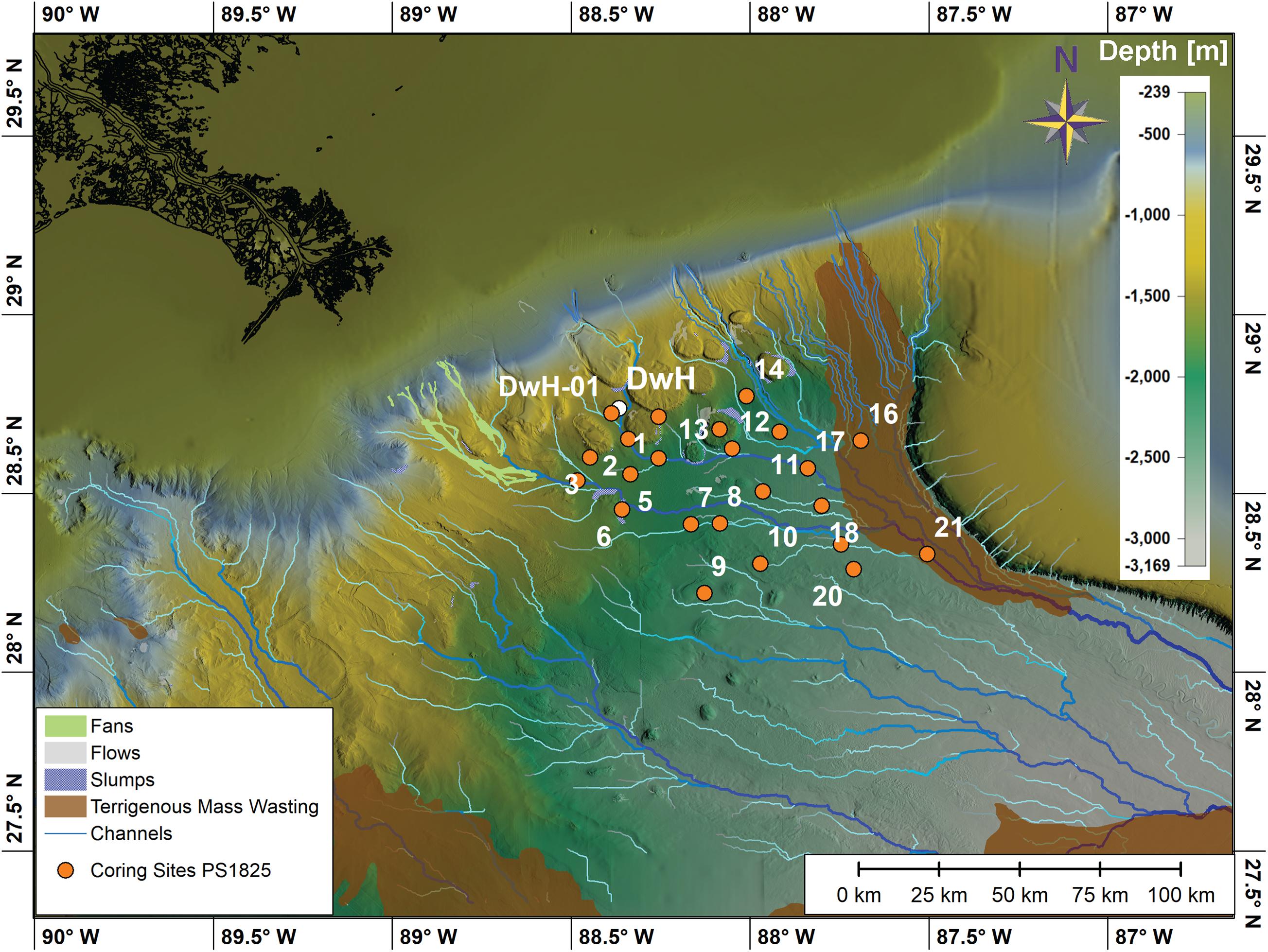
Figure 1. Location of coring sites with watershed model results (blue shaded lines). Included are geomorphological and sedimentological data from the Bureau of Ocean Energy and Management (BOEM). These data include locations of flows, fans, and terrigenous mass wasting areas, slumps, and channels.

TABLE 1

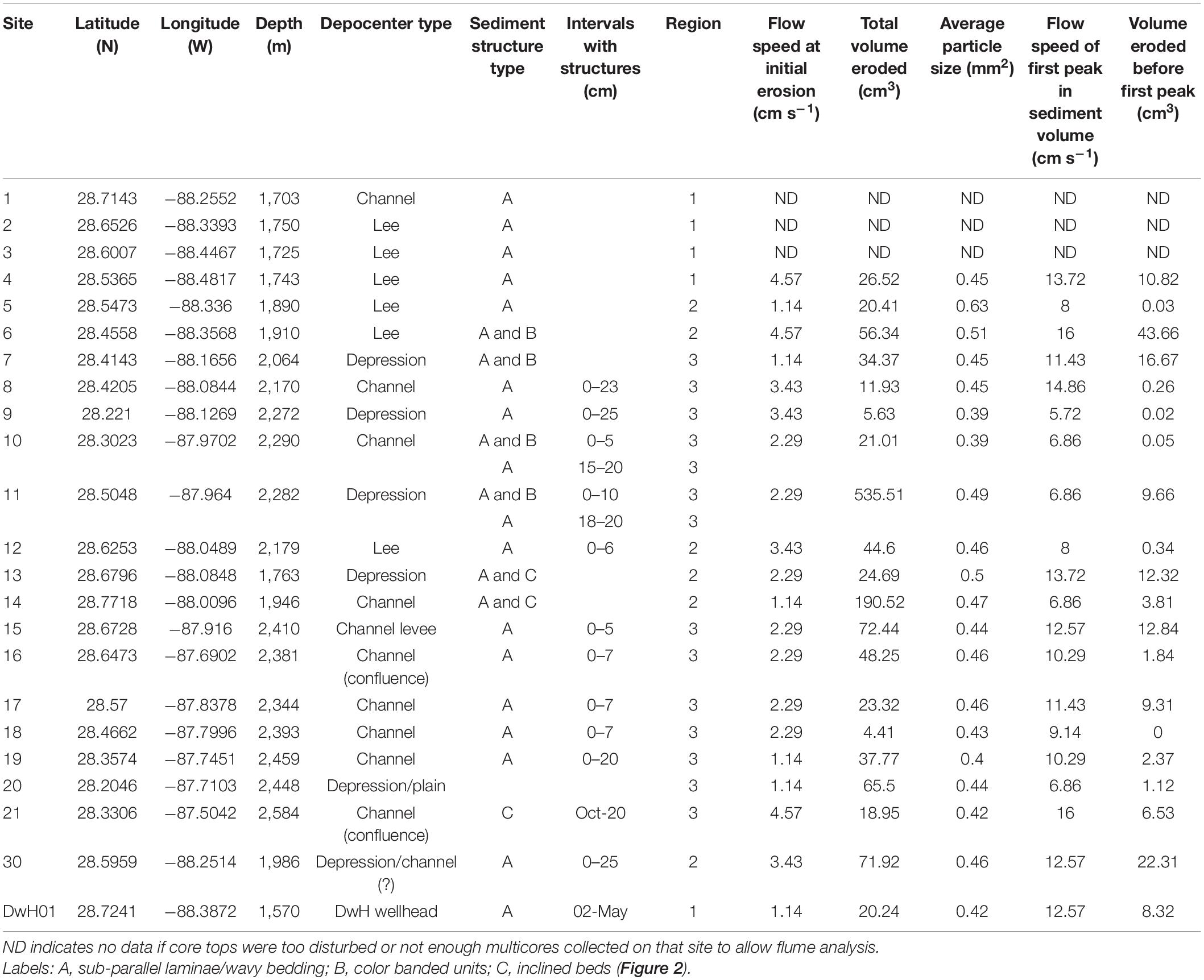
Table 1. Table of morphological classification and flume experiment data with surface sediment properties.

Collection of Sediment Cores

Sediment samples were collected during the RV Point Sur cruise 18–25 in May of 2018, using a MC-800 multi corer (10 cm diameter × 70 cm long tubes) at the studied sites (Figure 1 and Table 1). The Ocean Instruments MC-800 multi corer collected eight cores simultaneously and each core was used for a separate analysis (e.g., one core for bulk isotope analyses, one for short-lived radioisotope geochronology and sedimentology, one for XRF scanning, two for flume studies, one for hydrocarbon biomarkers, one for foraminiferal analyses, and one archived).

Sediment Resuspension Flume

To analyze resuspension behavior of the core samples, a linear closed loop flume was constructed. The resuspension flume (Supplementary Figure 1) was designed based on the Sedflume published by Borrowman et al. (2006). A 95 cm long 15 cm wide and 5 cm high closed channel was connected to a reservoir, through 5 cm diameter PVC pipes. In the upstream section of the flume, a DIGITEN model FL-1608 Hall Sensor flowmeter was installed in line before the flow diverter that converted the 5 cm PVC pipe into the rectangular test section of the flume. This flow diverter together with 147 cm of rectangular channel before the core insertion point allowed for full development of turbulent flow within the rectangular channel. At 147 cm beyond the flow diverter, a 10 cm diameter core opening was located at the base of the flume, allowing for insertion of the core into the flume. At the end of the rectangular section, another diverter reduced the diameter back to a 5 cm pipe through which the water was directed into a filtration system and the filtered, clean water was returned by the pump into the flume channel, thus creating the closed loop system.

A core extruding mechanism secured the core tube in the bottom of the flume during the test and permitted smooth controlled and undisturbed insertion of the core sediment into the flume. Cores had been collected and stored with a large amount of original seawater in the core tube overlying the sediment water interface. The flume was filled with filtered artificial salt water (salinity ∼ 35) prior to each test, and drained and cleaned after each experiment. The closed loop system provided an instantaneous movement of water within the entire flume when the pump was turned on.

During each test, a Sony 4k camcorder, mounted 20-cm beyond the core, with its focal point set at the center of the channel, recorded video data of calibrated particle size distribution of the material being eroded from the core top and transported down-channel. Time synchronized video footage was post processed using the GNU software FFMPEG into individual tagged image format files (TIF). For every 30 frames (video recorded at 30 frames per second), four images were extracted evenly spaced for every second of video time. Given the dimensions of the camera to the flume setup, this allowed for particles to be imaged in at least three consecutive images at the highest flow speed. Once all TIF images were extracted, they were analyzed using the Image Pro Plus^® software. All images were normalized into 8-bit gray scale images. A standard area of interest (AOI) with calibrated known dimensions was extracted from the image. The AOI was saved as separate file. The next image in time was loaded normalized, had the AOI applied and saved. During the following step, the first AOI was subtracted from the second AOI, leaving in the resulting image only particles that had shifted (moved within the channel) in position. Every stationary object was removed in the image subtraction process. All visible particles in the resulting image were counted and grouped into 10 size bins ranging from 0.2 mm² to >1.8 mm² in 0.2 mm² steps.

Core Splitting and Extrusion

With the exception of the flume cores, sediment cores were either split longitudinally or extruded upward from the core base for sampling. Sediment cores were extruded at 2 mm intervals for surficial sediment (2–10 mm) to ensure the highest possible resolution of recently deposited sediments, and subsequently at 5 mm intervals to the base of the core. Cores were volumetrically extruded according to the method described in Schwing et al. (2016). One core from each deployment was split longitudinally, photographed and described visually. This included assessment of stratigraphic integrity and a variety of sedimentary structures that are indicators of down-slope transport mechanisms.

Short-Lived Radioisotopes

Short-lived radioisotope analyses were performed to provide age control and accumulation rates over the past ∼100 years. Samples were analyzed for short-lived radioisotopes by gamma spectrometry on Series HPGe (High-Purity Germanium) Coaxial Planar Photon Detectors for activities of total Lead-210 (²¹⁰Pb_Tot) at 46.5 kiloelectron volts (keV), Lead-214 (²¹⁴Pb) at 295 keV and 351 keV, Bismuth-214 (²¹⁴Bi) at 609 keV, and total Thorium-234 (²³⁴Th_Tot) at 63 keV. Samples were also analyzed for Cesium-137 (¹³⁷Cs) at 661 keV, and Berilium-7 (⁷Be) at 477 keV, but these radioisotopes were below detection in all samples and therefore will not be discussed. Data were corrected for emission probability at the measured energy, counting time, sample mass, and converted to activity (disintegrations per minute per gram, dpm/g), using the International Atomic Energy Association (IAEA) organic standard IAEA-447 for calibration (Kitto, 1991; Larson et al., 2018).

The activities of the ²¹⁴Pb (295 keV), ²¹⁴Pb (351 keV), and ²¹⁴Bi (609 keV) were averaged as a proxy for the Radium-226 (²²⁶Ra) activity of the sample or the “supported” Lead-210 (²¹⁰Pb_Sup) that is produced in situ (Smith et al., 2002; Baskaran et al., 2014; Swarzenski, 2014). The ²¹⁰Pb_Sup activity was subtracted from the ²¹⁰Pb_Tot activity to calculate the “unsupported” or “excess” Lead-210 (²¹⁰Pb_xs), which is used for dating within the last ∼100 years.

The Constant Rate of Supply (CRS) algorithm was employed to assign specific ages to sedimentary intervals within the ²¹⁰Pb_xs profile. The CRS algorithm is appropriate under conditions of varying accumulation rates (Appleby and Oldfield, 1983; Binford, 1990). Mass accumulation rates (MAR) were calculated for each data point (i.e., “date”), based upon the CRS model results. The use of MAR corrects for differential sediment compaction down core, thereby enabling a direct comparison of ²¹⁰Pb_xs accumulation rates throughout a core (i.e., over the last ∼120 years). MAR were calculated as follows:

$MAR(g/cm{}^2/year)=drybulkdensity\times LAR(1)$

Where:

$\begin{array}{c}\hfill Drybulkdensity(g/cm{}^3)=sampledrymass(g)\\ \hfill ÷samplevolume(cm{}^3)\end{array}(2)$

$LAR=linearaccumulationrate(cm/year)(3)$

²¹⁰Pb_xs profiles were evaluated for the number of plateaus, the accumulation (mm) that was associated with plateaus e.g., accumulated as a pulse events, and the % of the total accumulation (mm) that occurred as a pulse. To quantify the accumulation for each core from episodic sedimentation a “Pulse Index” (P.I.) was calculated with the number of plateaus contributing 15% toward the index, the % of total accumulation that occurred with pulses (plateaus) contributing 50% toward the index, and the average MAR (1950–2018) contributing 35% toward the index (Supplementary Table 1 and Supplementary Figure 2).

Sedimentology

Sediment texture and composition analyses were conducted on extruded samples and included bulk density, grain size, and composition. One core per site was used to calculate pore water content and bulk density. Sample volume was calculated using the inner diameter of the core barrel and sampling interval (i.e., height). Samples were weighed immediately after extrusion to provide the wet mass required for determining pore water content. Each sample was then freeze-dried and weighed for dry mass to calculate dry bulk density (Binford, 1990; Appleby, 2001).

Grain size was determined by wet sieving the sample through a 63 μm screen. The fine-size (<63 μm) fraction was analyzed by pipette (Folk, 1965) to measure the relative percentage of silt (%silt) and clay (%clay). The sand-size (>63 μm) fraction was volumetrically too small to analyze further and is reported here as %sand. %Gravel and %sand were determined by dry sieving the >63 micron fraction. Carbonate content (%carbonate) was determined by the acid leaching method according to Milliman (1974). Total organic matter (%TOM) was determined by loss on ignition (LOI) at 550°C for at least 2.5 h (Dean, 1974). The non-carbonate and non-organic fraction is reported here as %terrigenous. Although, technically this fraction may include non-terrigenous components such as biogenic silica, glauconite and volcanic ash, they are only found in trace amounts in this general area (Stow et al., 1986), as Mississippi River input is such a dominant sediment source.

Carbon Isotopes

Samples for bulk isotopic analyses were treated with 10% HCl to remove carbonates, rinsed with DI water, freeze dried, and then ground with mortar and pestle prior to isotope analyses. Stable carbon (δ¹³C, %C) was measured using a Carlo-Erba elemental analyzer coupled to an isotope ratio mass spectrometer at the University of Maryland Center for Environmental Science Chesapeake Biological Laboratory. Samples were prepared for measurement of natural abundance of radiocarbon at the National High Magnetic Field laboratory. Acid treated sediment was combusted in quartz tubes at 850°C for 4 h and then the pure CO₂ was collected on a vacuum line using a series of cold traps to remove water vapor and non-condensable gases following the methods of Choi and Wang (2004). The purified CO₂ was flame sealed in a 6 mm ampoule and sent to Woods Hole National Ocean Sciences Accelerator Mass Spectrometry where the samples were prepared as graphic targets and analyzed by accelerator mass spectrometry (Vogel et al., 1984). The radiocarbon signatures are reported in Δ¹⁴C notation as described by Stuiver and Polach (1977). The ¹⁴C blanks were generally between 1.2 and 5 μg of carbon, producing a negligible effect on samples, which were over 1200 μg of carbon. The analysis of 22 replicate sediment samples yielded an average analytical reproducibility of ±6.8‰ for Δ¹⁴C and 0.2‰ for δ¹³C. Forty coal samples, representing fossil ¹⁴C dead carbon, were analyzed to access our procedural blank of combustion, graphitization, and target preparation, over the course of this study. The average Δ¹⁴C value was −995 ± 7‰. We also ran 25-azalea leaf standards collected in Tallahassee, Florida in 2013; the average Δ¹⁴C value was 31 ± 8‰.

Benthic Foraminifera

Following extrusion (methods provided above), five sub-samples from the surface of the sediment cores (0–2, 2–4, 4–6, 6–8, and 8–10 mm) and one sub-sample from down-core (20–22 mm) were used for benthic foraminifera analysis following methods similar to Schwing et al. (2018). Briefly, sub-samples were weighed and washed with a sodium hexametaphosphate solution through a 63-μm sieve to disaggregate detrital particles from foraminiferal tests (Osterman, 2003). The fraction remaining on the sieve (>63-μm) was dried in an oven at 32°C for 12 h, weighed again, and stored at room temperature (Osterman, 2003). Between 200 and 400 individuals from each subsample were identified to the species-level and counted. The fraction of the sample that was identified was then weighed. It was necessary to count between 200 and 400 individuals per sample to distinguish 2% significant variability in density and relative abundance between sample intervals (Patterson and Fishbein, 1989). Multiple taxonomic references were used (d’Orbigny, 1826, 1839; Williamson, 1858; Jones and Parker, 1860; Parker and Jones, 1865; Brady, 1878, 1879, 1884; Cushman, 1922, 1923, 1927; Stewart and Stewart, 1930; Phleger and Parker, 1951; Parker et al., 1953; Parker, 1954). The number of specimens with visibly fractured tests was counted and reported as the fracture percentage versus the total number of specimens identified as a taphonomical indicator of turbulent flow redistribution (Ash-Mor et al., 2017).

Hydrocarbon Analyses

Samples were kept frozen until freeze-dried at the Marine Environmental Chemistry Laboratory (MECL, College of Marine Science, University of South Florida). Approximately 1.0 g of freeze-dried and homogenized sediment was extracted using an Accelerated Solvent Extraction system (ASE^® 200, Dionex) under high temperature (100°C) and pressure (1500 psi) with hexane:dichloromethane (9:1 v:v). Deuterated standards were added to samples prior to extraction to monitor matrix effects and correct for losses during extraction (d10-acenaphthene, d10-phenanthrene, d10-fluoranthene, d12-benz(a)anthracene, d12-benzo(a)pyrene, d14-dibenz(ah)anthracene, d₅₀-tetracosane, d₁₅–pentadecane, d₃₂–dotriacontane, d₄-cholastane). For extraction in the ASE, we applied a one-step extraction and clean up procedure using a predetermined packing of the extraction cells (Kim et al., 2003; Choi et al., 2014; Romero et al., 2018) using a 11 ml extraction cell with glass fiber filter (pre-combusted at 450°C for 4 h), 5 g silica gel (high purity grade, 100–200 mesh, pore size 30A, Sigma Aldrich, United States; pre-combusted at 450°C for 4 h, and deactivated 2%), and sand (pre-combusted at 450°C for 4 h). Sediment extracts were concentrated to ∼2 ml in a RapidVap (LABONCO RapidVap^® Vertex^TM 73200 series) and further concentrated to about 100–300 μl by gently blowing with a nitrogen stream. An internal standard was added (d14-terphenyl; Ultra Scientific ATS-160-1) to all samples prior to GC/MS analysis. All solvents used were at the highest purity available. Two extraction control blanks were included with each set of samples (18 samples).

We followed modified EPA methods and QA/QC protocols (8270D, 8015C). Targeted compounds included aliphatics (C12–C37 n-alkanes, isoprenoids), PAHs (2–6 ring polycyclic aromatic hydrocarbons including alkylated homologs), and biomarkers [C27–C35 hopanoids, C27–C29 steranes, C20–C28 triaromatic steroids (TAS)]. Hydrocarbon compounds were quantified using GC/MS/MS (Agilent 7680B gas chromatograph coupled with an Agilent 7010 triple quadrupole mass spectrometer) in multiple reaction monitoring mode (MRM) to target multiple chemical fractions in one-run-step. Molecular ion masses for hydrocarbon compounds were selected from previous studies (Romero et al., 2015, 2018; Sørensen et al., 2016; Adhikari et al., 2017) (Supplementary Tables 2a,b). All samples were analyzed in splitless injections, inlet temperature of 295°C, constant flow rate of 1 ml/min, and a MS detector temperature of 250°C using a RXi-5sil chromatographic column. The GC oven temperature program was 60°C for 2 min, 60°C to 200°C at a rate of 8°C/min, 200°C to 300°C at a rate of 4°C/min and held for 4 min, and 300°C to 325°C at a rate of 10°C/min and held for 5 min. Source electron energy was operated at 70 eV, and argon was used as the collision gas at 1 mTorr pressure.

For accuracy and precision of analyses we included laboratory blanks for every 12–14 samples, spiked controls for every 14–18 samples, tuned MS/MS to PFTBA (perfluorotributylamine) daily, checked samples with a standard reference material (NIST 2779) daily, and reanalyzed sample batches when replicated standards exceeded ±20% of relative standard deviation (RSD), and/or when recoveries were low. Recovery ranged within QA/QC criteria of 50–120%. PAH concentrations are reported as recovery corrected. Each analyte was identified using certified standards (Chiron S-4083-K-T, Chiron S-4406-200-T, NIST 2779) and performance was checked using a 5-point calibration curve (0.04, 0.08, 0.31, 1.0 ppm). Quantitative determination of compounds was conducted using response factors (RFs) calculated from the certified standard NIST2779. Hydrocarbon compounds are expressed as sediment dry weight concentrations.

Hydrocarbon Source Identification

We used a tiered analytical approach for the identification of hydrocarbon sources in the sediment samples collected. First, we determined the concentration of hydrocarbon groups in the sediment samples (aliphatics, PAHs, and biomarkers (hopanoids, steranes, and TAS) to establish temporal (as profiles) and spatial (surface maps) changes of hydrocarbon concentrations and composition. Second, we determined and compared diagnostic oil ratios between potential sources and the samples (for details see below). Third, we compared the distribution pattern of n-alkanes and PAHs among samples.

Diagnostic oil ratios were calculated for all crude oil standards (NIST Macondo oil: MC252; Southern Louisiana Sweet crude oil: LC; southern GoM Akal Bravo oil: AB) and samples to discriminate hydrocarbon sources. Careful should be taken when applying diagnostic ratios to deep-sea sediments because of multiple weathering processes affecting the composition of hydrocarbons during sinking through the water column and after reaching the seafloor. For example, low molecular weight PAHs (LMW, containing 2–3 ring PAHs) are abundant in petrogenic sources while high molecular weight PAHs (HMW, containing 4–6 ring PAHs) are abundant in pyrogenic sources. However, HMW PAH can become more abundant due to the loss of LMW PAHs during weathering processes (e.g., dissolution, biodegradation). Alkane ratios were used to identify natural vs. oil sources (carbon preference index: CPI (C25–C33) = Σodd Cn/Σeven Cn) if samples were weathered (low molecular weight alkanes: % n-alkanes = ΣC14–C24/sum (C12–C37)^∗100). Samples with CPI < 2.0 and % n-alkanes < 25% indicate a weathered petrogenic source (Xing et al., 2011; Romero et al., 2015, 2021; Herrera-Herrera et al., 2020).

Other compounds, more resistant to weathering, can be used to identify specific oil sources (hopanes, steranes, triaromatic steroids). However, diagnostic oil biomarker ratios (using hopane, sterane, and triaromatic steroid compounds) known to fingerprint DwH oil or other crude oils have mostly been tested in samples collected from coastal environments (Wang and Fingas, 2003, Wang et al., 2006; Mulabagal et al., 2013; Aeppli et al., 2014) and a few in deep-sea sediments (Romero et al., 2015, 2017; Stout et al., 2016). In addition, some of these biomarker compound groups (e.g., steranes) have been shown to degrade in the marine environment years after an oil spill (Wang et al., 2001; Prince et al., 2002; Gros et al., 2014). Therefore, we tested if biomarker ratios used in previous studies (Wang and Fingas, 2003, Wang et al., 2006; Mulabagal et al., 2013; Aeppli et al., 2014; Romero et al., 2015, 2017) can be used to fingerprint deep-sea sediments, where organic matter and oil residues are naturally exposed to long-term weathering processes. Specifically, we compared the MC252 oil standard (NIST 2779) with samples collected at the DwH site (DwH-01), an area known to contain weathered oil residues from the DwH spill (Chanton et al., 2015; Romero et al., 2015; Stout et al., 2016). Also, samples from the DwH-01 site, the closest site to the DwH wellhead, sampled from 2011 to 2013, showed the presence and preservation of oil residues in the sediments from the DwH spill (Romero et al., 2017).

Only diagnostic ratios with a difference within ±20% between samples from site DWH-01 and the average of MC252 oil standard (N = 60) were used. In previous fingerprinting studies, this criteria for the difference between samples and an oil standard has been established based on the relative standard deviation value (RSD: 14–20%) of a standard analyzed over a period of time (analytical uncertainty) (Aeppli et al., 2014; Meyer et al., 2017). Our analysis of biomarkers using GC/MS/MS-MRM had an RSD of 4.8% over a time period of 6 months using the MC252 oil standard. The application of GC/MS/MS-MRM increases selectivity, improved baseline and signal-to-noise ratio, and successfully separates target compounds from interferences compared to the conventional GC/MS-SIM method (Adhikari et al., 2017). Altogether, the GC/MS/MS-MRM method improves the analytical uncertainty in the analysis of biomarker compounds. However, environmental sample replicates collected in deep-sea areas of the GoM have shown that RSD varies between 4% to 22% for biomarker compounds, indicating natural variability in the area (Romero et al., 2015). Therefore, diagnostic biomarker ratios of DwH oil residues at depth were selected using the RSD value of 20%, to account for the natural variability in deep sea environments. Ratios with a difference within ±20% between samples from site DWH-01 and the average of MC252 oil standard seem resistant to weathering and other natural processes at depth in the GoM, and are suitable for fingerprinting. The matching ratios were then calculated for all sites studied and analyzed using a Principal Component Analysis (PCA; JMP^® Pro 14.0). Also, cross plots of alkane diagnostic ratios were done to identify oil vs. natural sources in the region. In addition, the relative abundance (%) of hydrocarbon groups was plotted for each site studied to identify areas with high content of LMW PAHs (2–3 rings) due to inputs from natural seeps.

Only samples indicating oil content (using alkane ratios), no natural seep inputs (with low %LMW PAHs), a distinct distribution pattern of n-alkanes and PAHs indicating weathered oil residues, and a match with the MC252 oil standard (using biomarker ratios) were identified to contain DwH oil residues as the most probable oil source.

Results

All sites yielded sediment cores with active deposition over the past ∼100 years. Core analyses revealed a range of sediment textures, composition and accumulation rates indicating that sedimentation processes varied throughout the study area. Downcore data were utilized for some analyses to provide a longer time-scale context (Figure 2) and to assess the historical prevalence of down-slope sediment transport as indicated by various sedimentary structures present throughout the study area. All other analyses focused on the surficial sediments (0–20 mm) to identify recent patterns that may be associated with deposition and redistribution of DwH contaminated sediments. We have provided maps in figures and supplementary figures as a mechanism to visualize the data and to communicate the observed variations in the data. Interpolations of data in the areas between the individual coring locations were dependent on parameters set in the contouring program (Golden Software Surfer 9.0) and were thus not discussed in this manuscript.

FIGURE 2

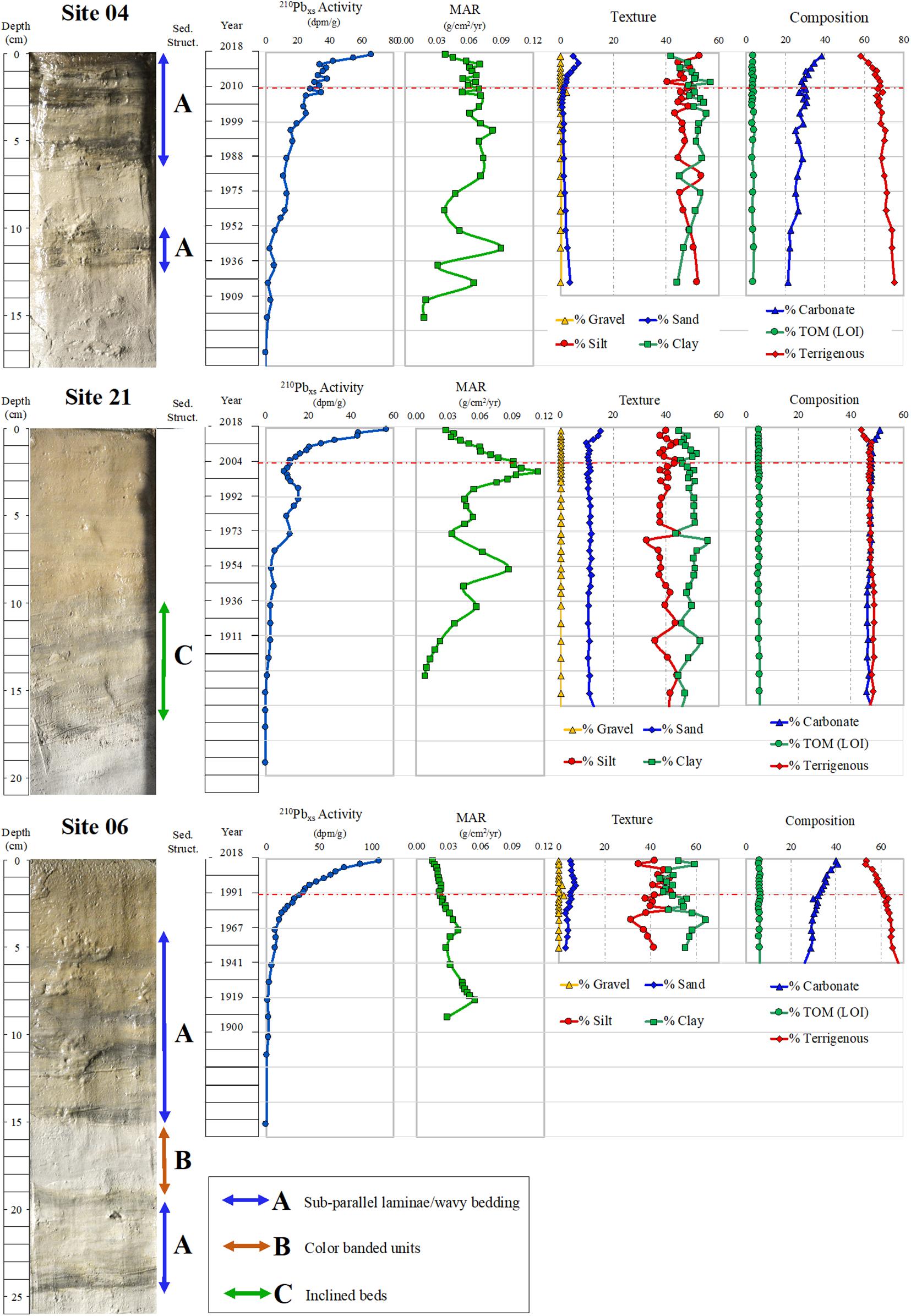
Figure 2. Core logs for Site 4 (Region 1), Site 6 (Region 2), and Site 21(Region 3) showing sedimentary structures indicative of sediment re-deposition by gravity flow processes, ²¹⁰Pb_xs profiles and MARs, and sediment texture and composition to assess historical prevalence of downslope sediment transport and accumulation. (Labels: A, sub-parallel laminae/wavy bedding; B, color banded units; C, inclined beds).

Flume

Flume experiments showed that sediment particle erosion behavior was not uniform across the various sedimentary environments on the seafloor (Table 1). The uppermost layer of sediment (top 2 mm) from each core eroded at different flow speeds, producing maximum peaks in total number of particle counts at flow speeds from 5.72 cm s^–1 to 16 cm s^–1 (Table 1 and Figure 3). Several sediment cores exhibited a second peak at higher flow speeds (sites 10, 11, 14, 17, and 20). In all cores (sites 8, 9, 10, 17, 19, and 20) that had a first peak in particle resuspension at low flow speeds, a decrease in resuspended particle concentration was observed following the initial peak resuspension of particles. A second larger peak, produced by a complete collapse of the surface sediment layer, occurred in all cores at flow speeds exceeding 13.7 cm s^–1. Sediments from cores that did not have the initial peak in resuspended particles (sites 4, 5, 6, 12, 13, 15, 16, 21, 30, and DwH-01) had low numbers of particles resuspended until a rapid disintegration of the surface sediment layer occurred >13.7 cm s^–1.

FIGURE 3

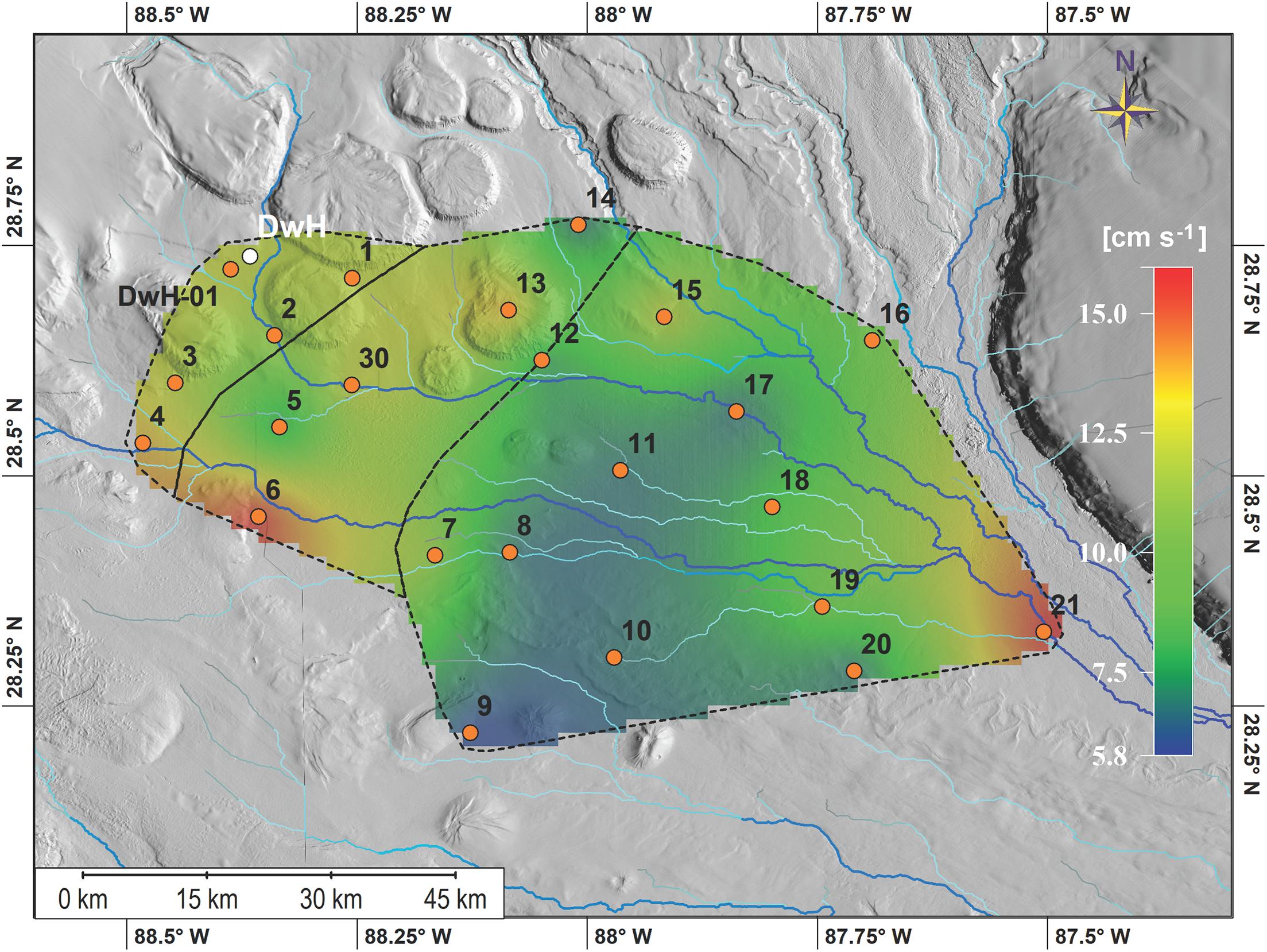
Figure 3. Heat map of flow speed of first peak in particle resuspension. Regions discussed are outlined by the dashed black lines. Region 1 is in the NW and Region 3 in the SE. Blue lines indicate channels as modeled by watershed analysis.

Distinct peaks in total volume with increased flow speed were recorded for each core analyzed. Average area of individually eroded particles varied only slightly between 0.39 and 0.63 mm² in all cores, however, total eroded volume of particles varied from 4.4 to 535 cm³ (Table 1).

Short-Lived Radioisotopes

Short-lived radioisotope analyses yielded ²¹⁰Pb_xs activity profiles utilized to provide age control and sedimentation rates at multicore sites over the past ∼120 years. ²¹⁰Pb_xs profile shape and MAR, averaged over various time periods, were used to characterize the spatial patterns of sediment distribution and accumulation.

²¹⁰Pb_xs activity profile shapes varied with some sites exhibiting exponential profiles and others non-exponential profiles (Figure 2 and Supplementary Figures 3a–c). Non-exponential profiles ranged from small mm-scale plateaus in activity to profiles with large cm-scale plateaus. Some profiles contained few plateaus, and some contained multiple plateaus. These profiles were utilized to assess the relative magnitude and frequency of episodic or pulsed accumulation (plateaus in activity in profiles) vs. areas with stable consistent accumulation (exponential profiles).

The spatial pattern of the pulse index reveals variability in the prevalence of sediment accumulation from episodic events over the past ∼120 years (Figure 4). In the northwestern portion of the study area (sites 1, 2, 3, 4, and DwH-01) a high index, reflecting frequent episodic sedimentation events, was observed. The central portion of the study area consists of low index values (sites 5, 6, 12, 13, 14, and 30) reflecting a more stable, consistent sediment accumulation history. The southeastern portion of the study area shows high index values (sites 7, 8, 9, 10, 11, 15, 16, 17, 18, 19, 20, and 21) but with the highest episodic sedimentation events observed in the study area, in terms of magnitude and frequency.

FIGURE 4

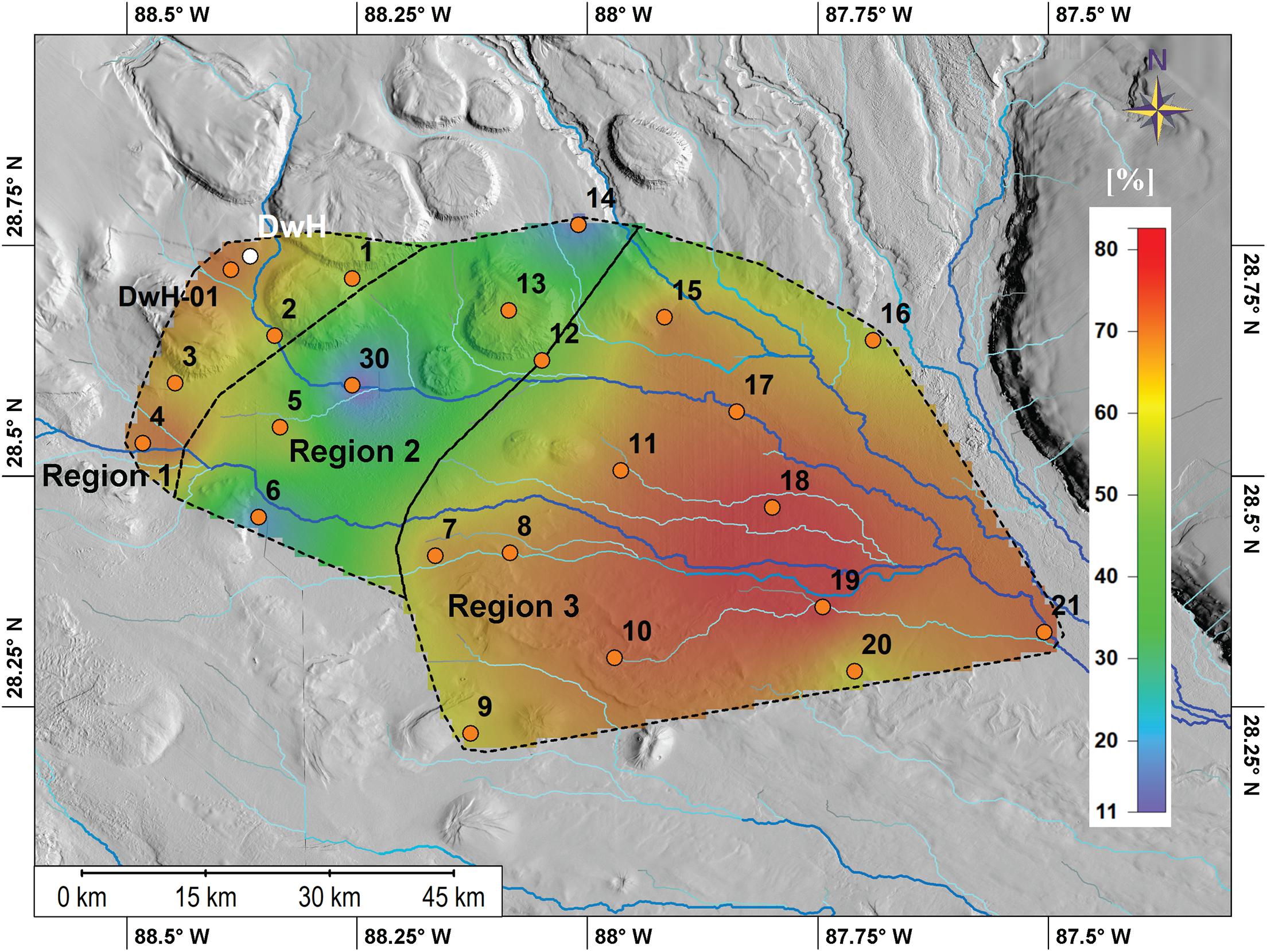
Figure 4. Heat map of weighted pulsed input in study area. The three regions identified in this study are marked by black lines and are labeled Region 1, 2, and 3 form the NW to the SE. Scale describes the percentage of pulsed inputs in the study area.

Sediment MAR’s were determined using ²¹⁰Pb_xs age dating. Differing time periods were evaluated to characterize accumulation rates from a long (1950–2018) to short periods for characterizing events pre-spill (2006–2009; Figure 5A), during and after the spill related to the MOSSFA event (2010–2013; Figure 5B), and post-spill associated to redistribution of sediments (2014–2018; Figure 5C). Spatial patterns of MAR’s from 1950 to 2018 are consistent with the areas of episodic sedimentation identified by the ²¹⁰Pb_xs pulse index, further corroborating the spatial variability in the influence of episodic sedimentation events (Figure 4). For the three recent time periods compared in this study, there are potential shifts in “hot spots” of higher accumulation with site 18 consistently being a “hot spot” for accumulation in all three periods. Site 9 shows increased MAR’s in the 2010–2013 time period. In the 2014–2018 period, there are higher MAR’s at site 16 near the base of the DeSoto Canyon as compared to the 2006–2009 and 2010–2013 time periods (Figures 5A–C).

FIGURE 5

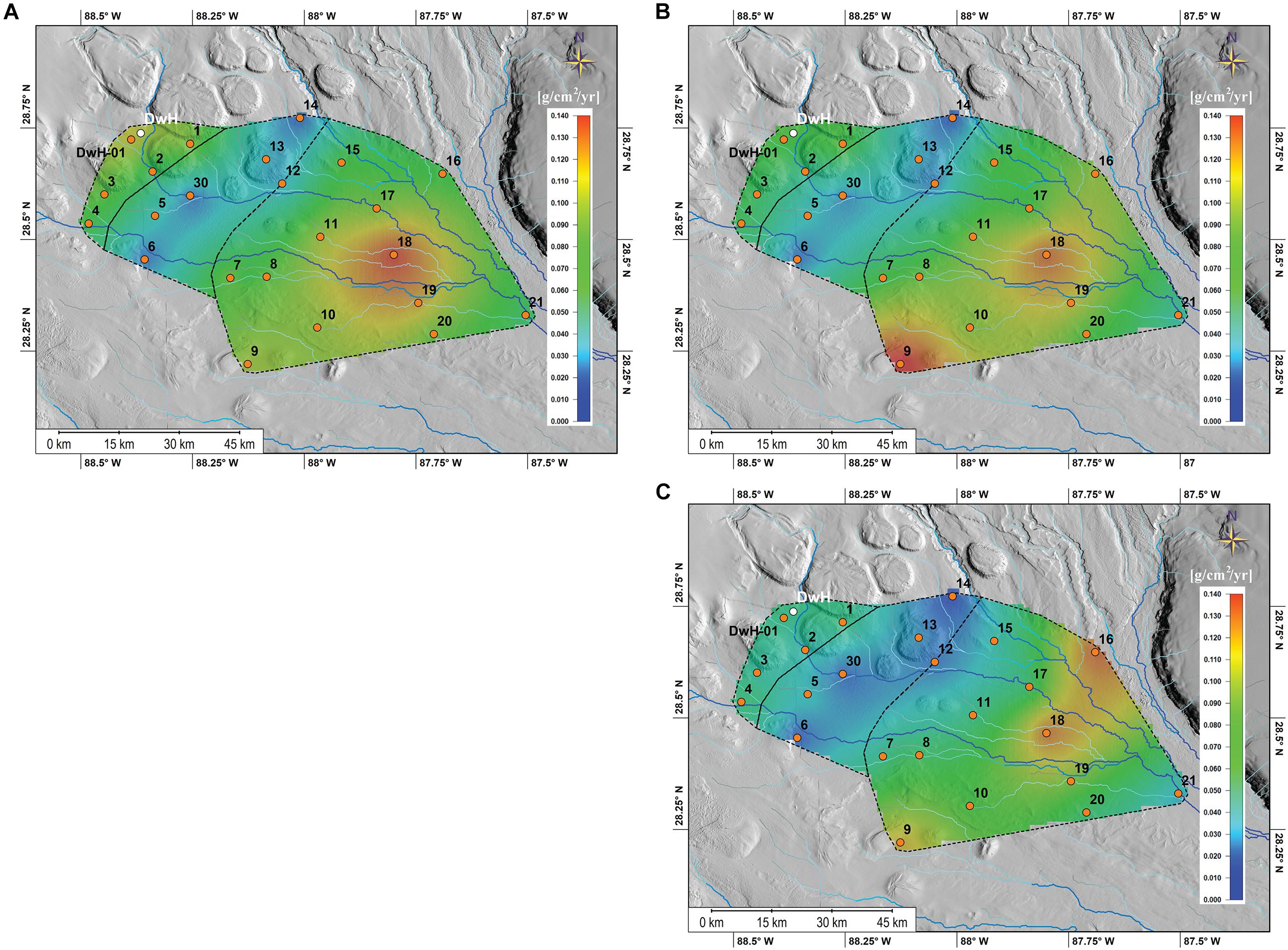
Figure 5. Heat maps of average sediment accumulation rates determined from ²¹⁰Pb_xs. (A) Pre-Spill (2006–2009), (B) 2010–2013, and (C) 2014–2018. Regions discussed are outlined by the dashed black lines. Region 1 is in the NW and Region 3 in the SE. Blue lines indicate channels as modeled by watershed analysis.

Sedimentology

All cores exhibited intact detailed stratigraphy, contained numerous, well-preserved primary sedimentary structures, and very few secondary sedimentary structures (e.g., bioturbation). The most common structures were thin, mm-scale, sub-parallel laminae and wavy bedded units with no clearly defined lower boundaries (Figure 2). These structures were found throughout the entire study area in all depocenter types (Table 1). Inclined and color banded beds (Figure 2) were less common, and sparsely dispersed throughout all but the northeastern-most portion of the study area (Table 1). Generally, sedimentary structures were better defined in the upper few 10’s of cm of cores (Table 1).

Sediment grain size and composition was averaged over the surficial 0–4 mm and 10 mm intervals and varies throughout the study area. Grain size is reported as %gravel, %sand, %silt, %clay, and %mud (%silt + %clay), and composition is reported as %carbonate, %TOM (total organic matter by LOI), and %terrigenous (Table 2 and Supplementary Figures 4–8). %Carbonate ranged from 45% to 60% with lowest concentrations in the NW portion of the study area and increasing to the SE. %TOM ranged from 4.4% to 7.1% with highest values in the NW and decreasing to the SE. Sediment grain size showed more spatial variability than composition. %Gravel was zero in all sites except site 03, which contained large pteropod fragments. %Sand ranged from 0.3% to 12.9% with highest values in the SE, lowest values in the N, and moderate values in the W portion of the study area. %Silt ranged from 35.3% to 58.5% with highest values in the NW, lowest values in the NE and SE, and modest in the SW portion of the study area. %Clay ranged from 39.9% to 63.3% with highest values in the NE, modest through the central to S, and lowest in the NW and SE areas. Highest %carbonate values were consistently associated with the highest %sand, which consisted of sand size biogenic carbonate particles (Supplementary Figures 4–8).

TABLE 2

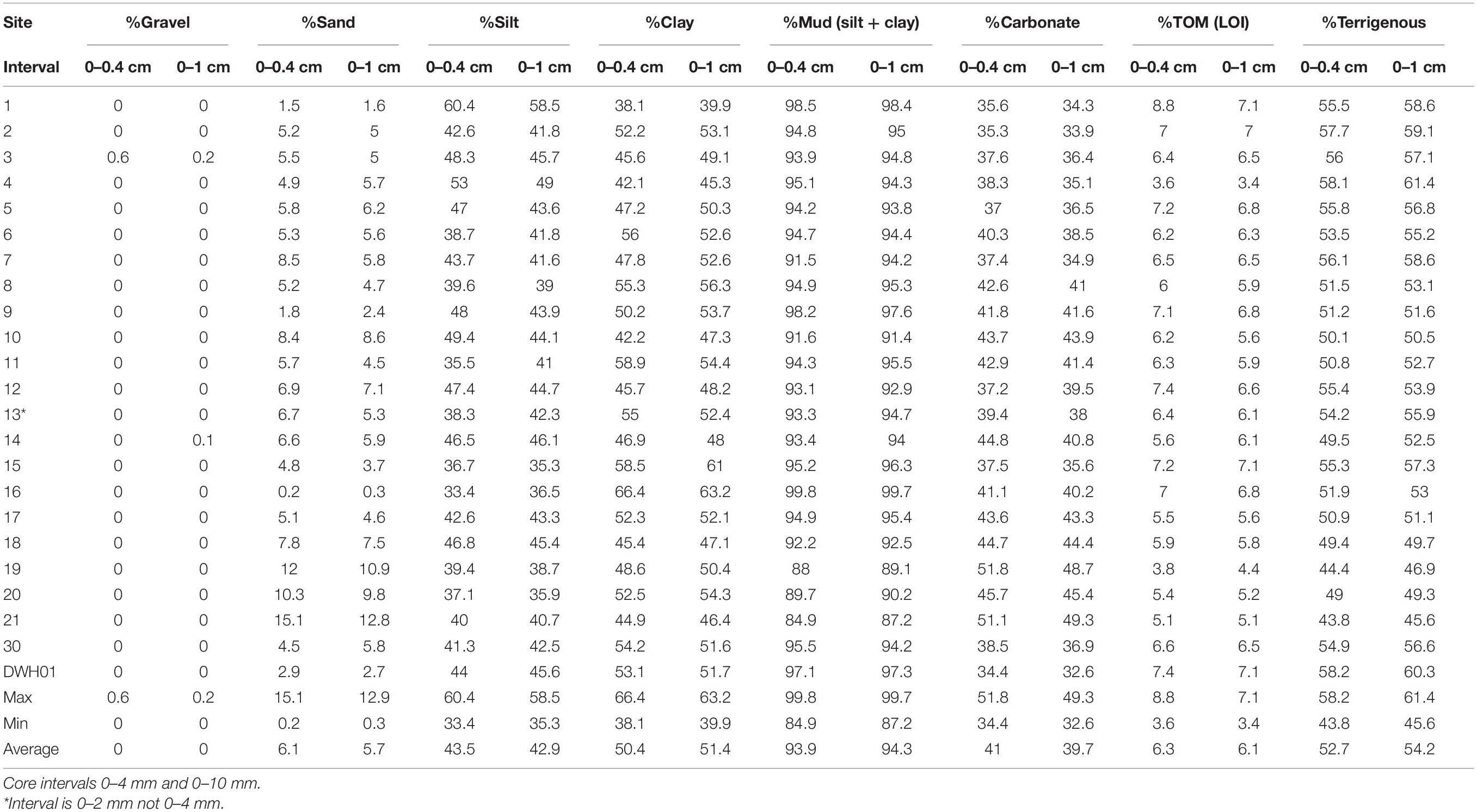
Table 2. Sedimentological data.

Carbon Isotopes

The sedimentary organic carbon content in percent carbon by weight, %C, the stable carbon isotopic composition, δ¹³C ‰, and the radiocarbon content, Δ¹⁴C ‰, of the surface 0–2 mm layer and the 0–10 mm layer are reported in Supplementary Table 3. Values for the 0–10 mm depth interval were calculated as the average of the five 2 mm slices subsampled within that interval. The %organic carbon of the uppermost interval (0–2 mm) varied from 1.3 to 2.9% and generally decreased from the northwest to the southeast as the water deepened (Figure 6). The δ¹³C of surface (0–2 mm) organic matter varied from −20.7 to −22.5‰ and was more depleted to the northwest and exhibited a minimum in the center of the study area (Figure 7). There was a significant correlation of increasing δ¹³C with decreasing %organic carbon (p = 0.01, r = 0.512, n = 24). Radiocarbon content in the surficial layer (0–2 mm) varied from −167 to −319‰ across the study area (Figure 8). The most depleted values were observed at about 2,300 m depth on the north east and western sides of the study area. The central portion of the study area exhibited ¹⁴C enriched surface sediments downslope of the DwH site, in water depths ranging from 1,700 to 2,100 m, grading to more depleted values to the southeast. None of these parameters correlated with depth.

FIGURE 6

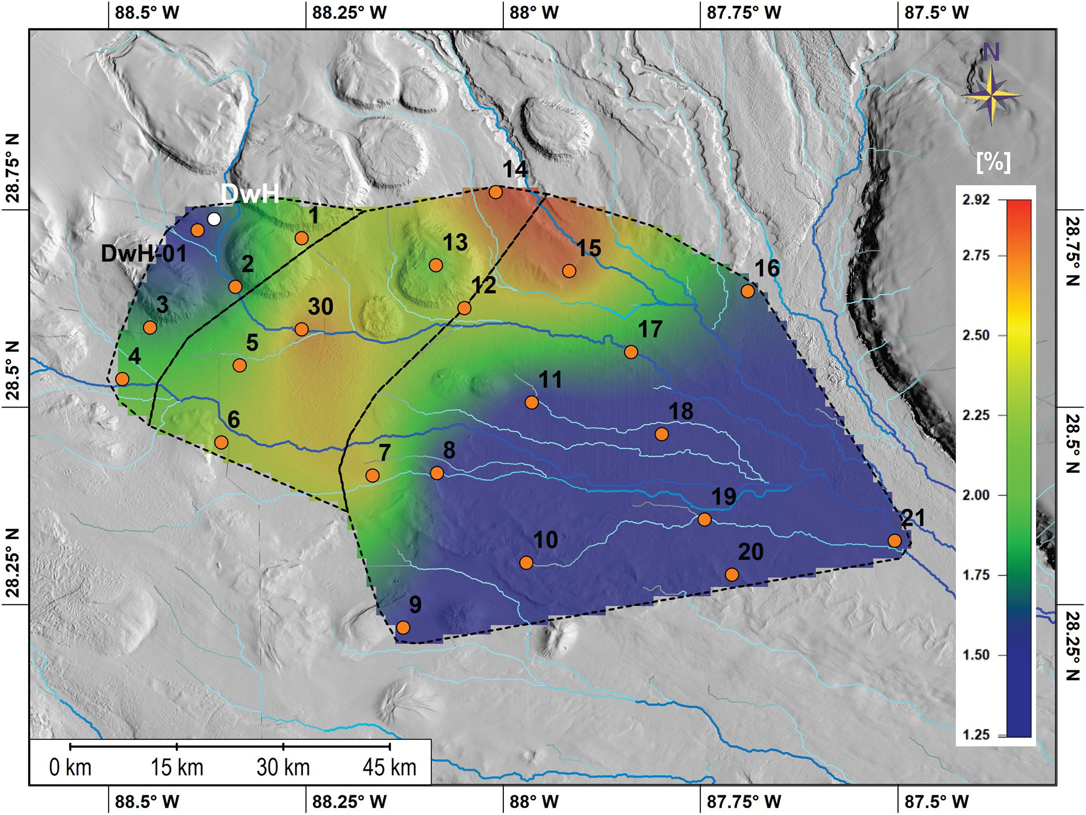
Figure 6. Heat map of %carbon content of the upper 2 mm of the cores. Regions discussed are outlined by the dashed black lines. Region 1 is in the NW and Region 3 in the SE. Blue lines indicate channels as modeled by watershed analysis.

FIGURE 7

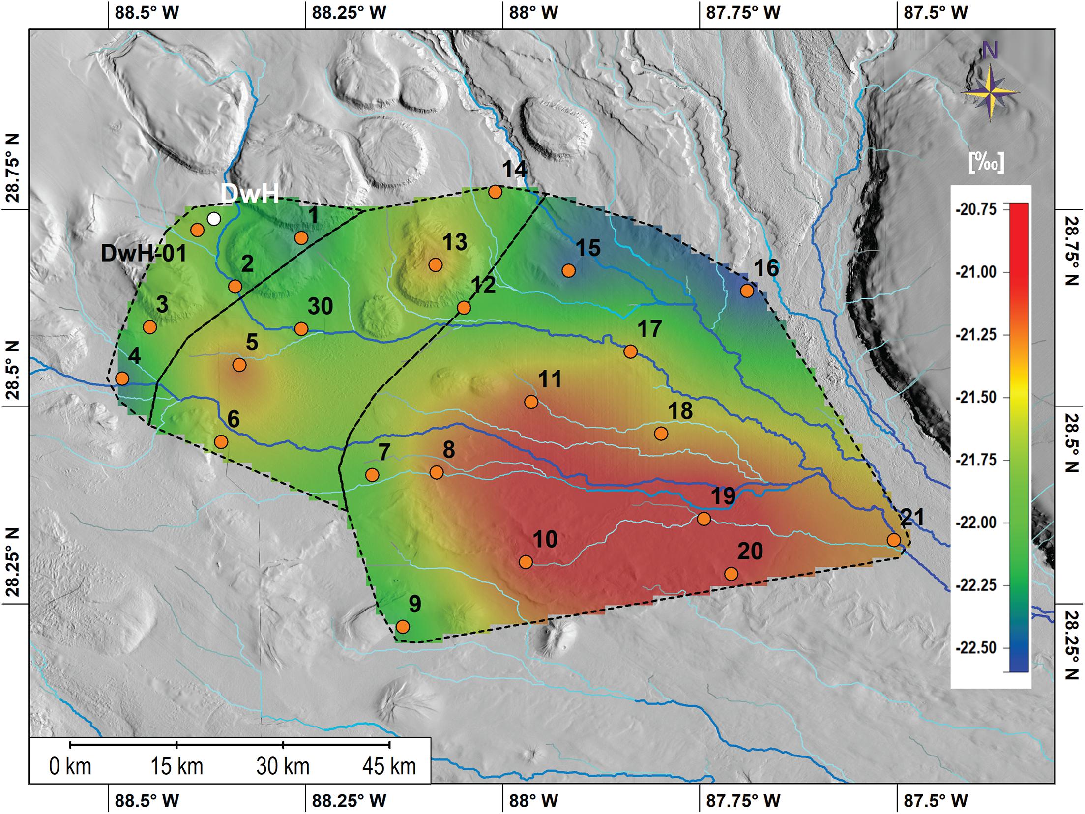
Figure 7. Heat map of δ¹³C surface isotopic composition (0–2 mm). Regions discussed are outlined by the dashed black lines. Region 1 is in the NW and Region 3 in the SE. Blue lines indicate channels as modeled by watershed analysis.

FIGURE 8

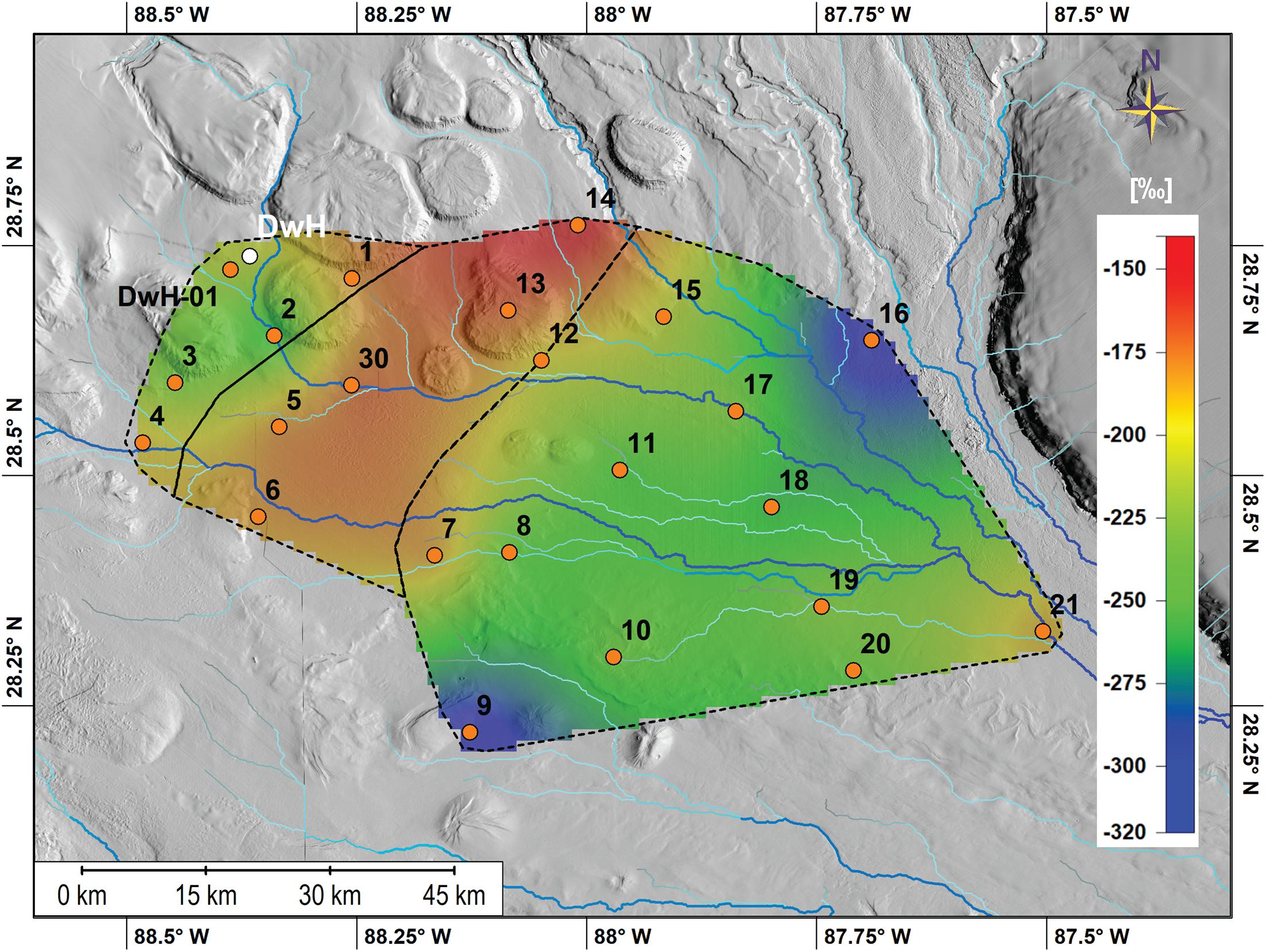
Figure 8. Heat map of Δ¹⁴C surface activity of the upper 2 mm of the cores. Regions discussed are outlined by the dashed black lines. Region 1 is in the NW and Region 3 in the SE. Blue lines indicate channels as modeled by watershed analysis.

Benthic Foraminifera

Benthic foraminifera density and fracture percentage are presented in Supplementary Table 4. Benthic foraminifera density ranged from 15 to 74 individuals/cm³ and generally increased from the northwestern (e.g., site 1 mean density: 19 individuals/cm³) to the southeastern (e.g., site 24 mean density: 38 individuals/cm³) portion of the study area. Benthic foraminifera fracture percentage ranged from 7.5 to 25.1% with the highest mean fracture percentage in the north-central portion of the study area (e.g., site 12 mean: 20.6%, site 14 mean: 16.0%). Maxima in fracture percentage were typically found at 6–10 mm depth (sites 1, 9, 12, and 16). These maxima were often coincident with variability in other parameters consistent with resuspension (Figure 9).

FIGURE 9

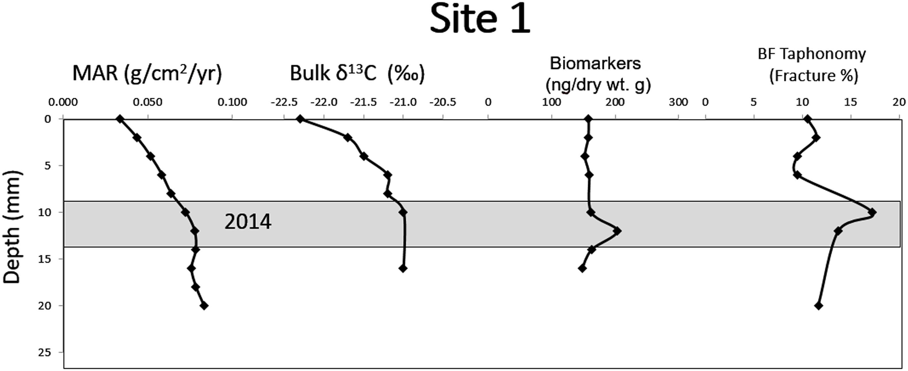
Figure 9. An example of the multi-proxy assessment from station MC01, where an event was identified between 10 and 12 mm depth (year 2014) by relatively high mass accumulation rates, homogenous bulk organic stable carbon isotopes, an maxima in organic biomarkers and benthic foraminifera fracture percentage.

Hydrocarbon Analyses

We identified 10 biomarker ratios that can be used as diagnostic biomarker ratios of DwH oil residues at depth (Figure 10). These biomarker ratios determined for samples from DWH-01 site lie within ±20% of the MC252 standard ratios. The fewer biomarker ratios that matched with the MC252 standard compared to coastal studies may indicate that more compounds are susceptible to multiple weathering processes at depth (e.g., dissolution, degradation, dispersion). Source apportionment of hydrocarbons in the study area after the spill was determined using principal component analysis (PCA) of the biomarker ratios identified in Figure 10. The PCA results in Figure 11 show that 46% of the sites in 2010–2013 and 58% of the sites in 2014–2018 contain oil-residues similar to the MC252 oil standard (all located in the same PCA space) and distinct from other reference oil samples from the GoM. PCA results are supported by cross plots of alkane diagnostic ratios (Figure 12) and %abundance plots of hydrocarbon compounds groups (Supplementary Figures 9a,b). Caution should be taken when interpreting deep-sea data, because oil-residues deposited at depth, regardless of the source, are highly weathered. For example, Figure 12 shows that several sites in both time periods (2010–2013: sites 1, 14, 8; 2014–2018: sites DwH-01, 1, 2, 12, 14, 16) contain oil-residues (CPI < 2.0 indicates oil-residues; %C14–C24 < 25% indicates heavily weathered samples) but with a dominant hydrocarbon source different than DwH oil, as shown by the PCA results (Figure 11). Also, some sites that were designated by the PCA to potentially contain mostly DwH oil-residues (shown in orange color sites 7 and 18 for 2010–2013, and sites 9 and 10 for 2014–2018) are shown in Figure 12 to be mixed with other sources different than oil-residues (e.g., terrestrial), therefore we have classified these sites to contain mixed sources of hydrocarbons (shown in orange color in Figures 11–13 and Supplementary Figures 10a,b). In addition, the results from the PCA analysis and cross plots were supported by distinct distribution patterns of n-alkanes and PAHs (Supplementary Figures 11, 12). The samples identified to contain DwH oil-residues as the potential major source for hydrocarbons in Figures 11, 12, have a distinct n-alkane composition with short-chain compounds (C12–C23) less than 2% abundance, while long-chain compounds (>C30) are more than 10% abundance (Supplementary Figure 11 and in agreement with Stout et al., 2016). This pattern is expected from severely weathered oil residues, in which long-chain n-alkanes are preserved due their lower susceptibility to dissolution and biodegradation. In contrast, other sources (as mixed or unknown in Supplementary Figure 11) show a strong odd-to-even carbon preference for long-chain n-alkanes, with C27, C29 and C31 as the most abundant. The observed odd-to-even carbon preference for long-chain n-alkanes is typical of terrestrial plants. For PAHs, the difference in distribution pattern among sources is as well observed (Supplementary Figure 12). The samples identified to contain DwH oil-residues as the potential major source for hydrocarbons in Figures 11, 12 have less %abundance of molecular markers of incomplete combustion such as Re and BeP (Ramdahl, 1983; Wang et al., 1999; Tobiszewski and Namieśnik, 2012), while 4–6 ring PAHs were more abundant due to their higher resistant to weathering processes such as dissolution and biodegradation. This pattern is more notorious by comparing the abundance of PAH compounds grouped by ring number (Supplementary Figure 13) showing a distribution difference among sources within each year. Also, larger changes between time periods is observed indicating potential additional weathering processing affecting mostly 5–6 ring PAHs (e.g., transformation processes, White et al., 2016). Overall, we found that 15 sites of the 24 studied sites contain DwH oil-residues as the potential major source for hydrocarbons (Figure 13). The results generated using multiple oil diagnostic ratios indicate the significance of using ratios from multiple compound groups (e.g., hopanes, steranes, alkanes, PAHs) for source apportionment of hydrocarbons in deep-sea areas, like in the northern GoM.

FIGURE 10

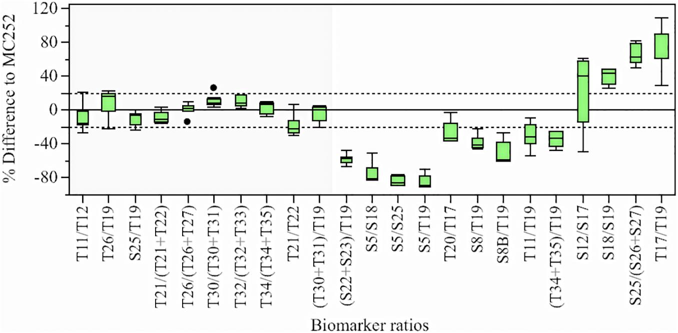
Figure 10. Relative difference of biomarker ratios from DW site to the crude oil standard MC252. Graph shows green boxes as the interquartile ranges, with horizontal lines indicating median values and whiskers representing the 10th and 90th percentiles. Black circles denote outlier values, and dotted horizontal lines indicate ratios within ±20% of the MC252 standard. Information of compounds can be found in Supplementary Tables 2a,b.

FIGURE 11

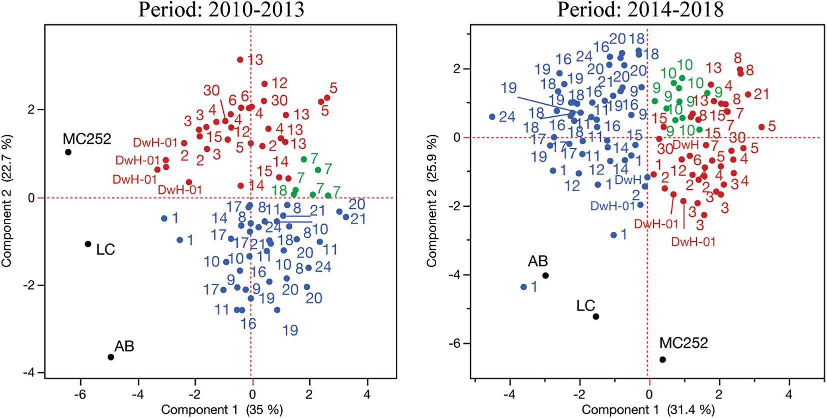
Figure 11. Discrimination of diagnostic ratios in the studied area by principal component analysis (PCA) for the 2010–2013 and 2014–2018 time periods. Black circles show oil reference oils from the GoM (MC252: DWH oil; AB: southern GoM Akal Bravo oil; LC: Southern Louisiana Sweet oil), numbers indicate sites, red circles denote sites with DWH oil-residues as the potential major source, green circles indicate sites with mixed hydrocarbons sources including DWH oil-residues, and blue circles indicate other unknown sources. The diagnostic ratios used are described in the method section.

FIGURE 12

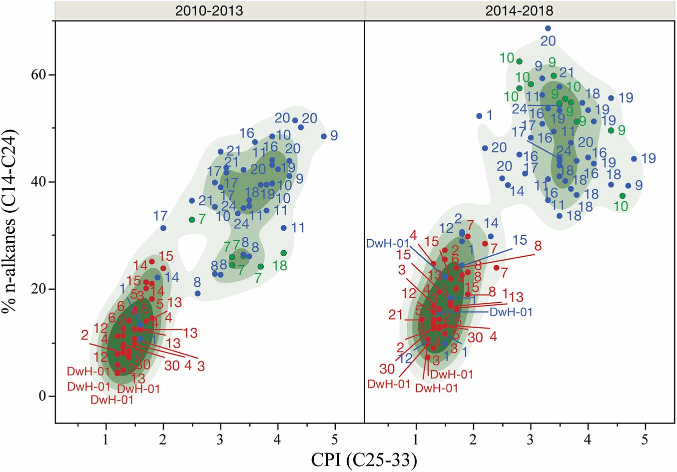
Figure 12. Cross plots of diagnostic ratios for the deep-sea sites studied in the northern GoM. Numbers indicate sites, red circles denote sites with DwH oil-residues as the potential major source, green circles indicate sites with mixed hydrocarbons sources including DwH oil-residues, and blue circles indicate other unknown sources.

FIGURE 13

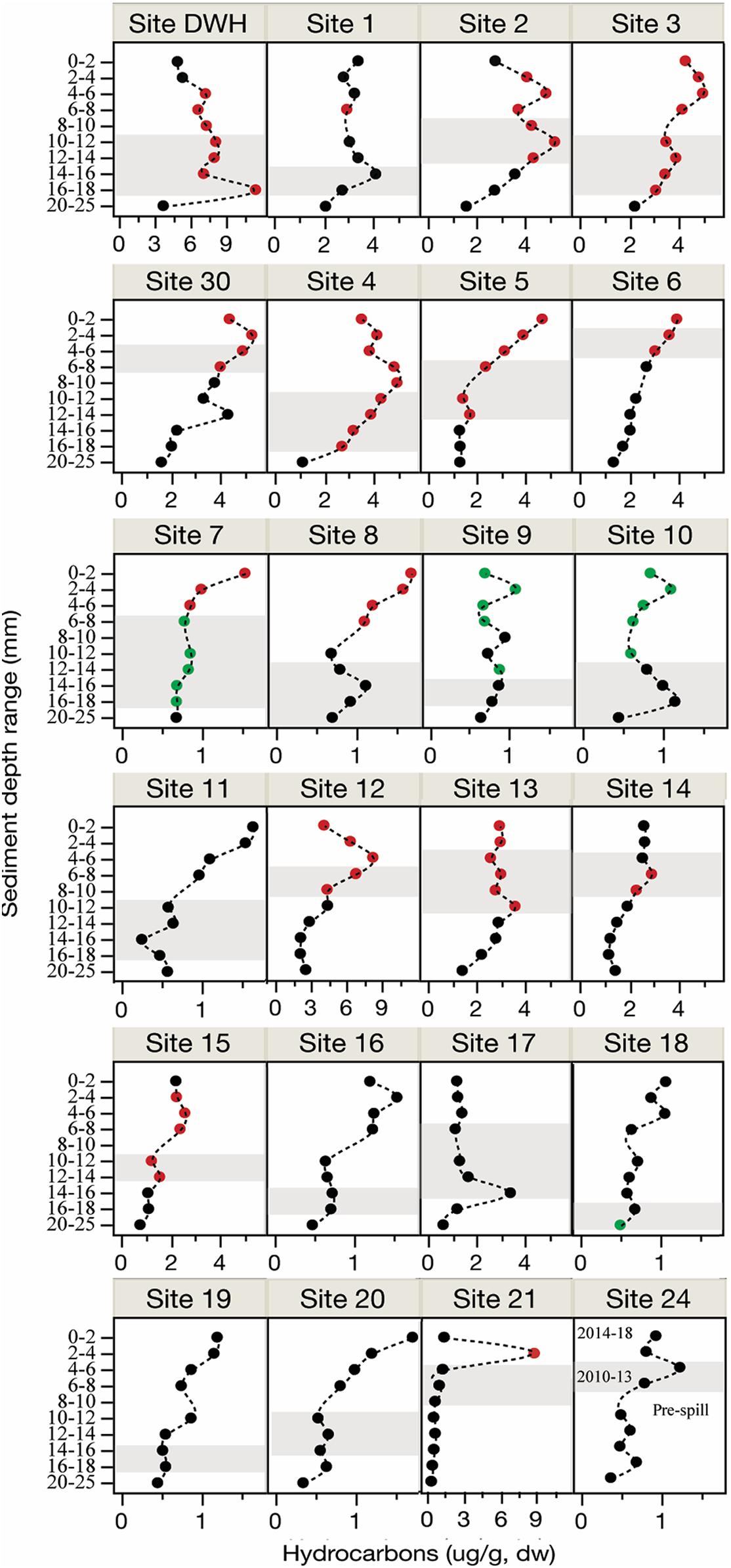
Figure 13. Profiles of hydrocarbon concentrations in the study sites located in the northern GoM. Hydrocarbons refer to the sum of aliphatics, PAHs, hopanes, steranes, and TAS. Graph shows shaded areas corresponding to the time period 2010–2013, areas above and below the gray area corresponds to 2014–2018 and pre-spill periods, respectively. Red circles denote samples with DwH oil-residues as the potential major source, green circles indicate samples with mixed hydrocarbons sources including DwH oil-residues, and black circles indicate other unknown sources.

Hydrocarbon concentrations, the sum of all compounds analyzed [n-alkanes, isoprenoids, polycyclic aromatic hydrocarbons (PAHs), hopanes, steranes, and triaromatic steroids (TAS)] ranged from 0.2 μg/g to 11.4 μg/g, with decreasing concentrations toward southeast of the study area, with some exceptions observed at specific depth layers in the sediments (e.g., site 21) (Figure 13). Specifically, hydrocarbon averages >2.0 μg/g were observed in the northeast of the study area (sites DwH, 1–6, 12, 13, and 30), concentrations in the range of 0.9–2.0 μg/g were detected at the center of the study area (sites 7, 8, 11, 14, 15, 16, and 17), and concentrations <0.9 μg/g were observed in the southeast area (sites 9, 10, 19, 20, 21). This general trend in hydrocarbon concentration followed sediment grain size distribution, with higher concentrations where sediments have low carbonate content. In addition, downcore profiles show a large variability in hydrocarbon concentrations in the study area, with enhanced concentrations at specific sediment intervals (Figure 12). Also, specific hydrocarbon compound groups did not show a clear trend with depth (e.g., decrease with sediment depth); therefore, compound relative abundances mostly represent changes in hydrocarbon sources rather than solely biodegradation of hydrocarbons after buried (Supplementary Figures 9a,b). Most abundant compound groups were n-alkanes and high molecular weight PAHs (HMW, 4–6 rings). Profiles of HMW PAHs and LMW PAHs (low molecular weight, 2–3 rings) showed large variability in some sites in all sediment depth layers (i.e., site 10) or at specific sediment layers (i.e., sites 1, 11, 17, and 19), but in all cases HMW PAHs were more abundant.

Discussion

Spatial Distribution

All sites were depositional over the past ∼100 years and to various degrees contained sedimentary structures, but there were distinctive variations in accumulation patterns and sediment characteristics throughout the study area. These variations define three distinctive geographic regions with implications for the degree of influence of down-slope sediment transport on sediment accumulation patterns (Figure 4). Bathymetric characteristics, geographic location, and water depth also play a role in the characteristics of each region. Defining characteristics of the regions include episodic vs. stable sediment accumulation patterns as well as surficial sediment characteristics (upper 0–10 mm of cores). Using ²¹⁰Pb_xs age dating, cores were assessed for accumulation patterns from 1950 to 2018 for longer term reference and in greater detail for three time periods, 2006–2009 (pre-spill), 2010–2013 (DwH spill/post-spill), and 2014–2018 (post-spill) to investigate the DwH spill and potential down-slope redistribution in subsequent years.

(a) Region 1 is in the NW portion of the study area directly surrounding the DwH spill site and includes our station DwH-01, and sites 1, 2, 3, and 4 (Figure 4).

(b) Region 2, includes sites, 5, 6, 12, 13, 14, 30, to the SE of Region 1, consisting of a “belt” running from the NE to SW (Figure 4).

(c) Region 3, SE of Region 2, includes sites 7, 8, 9, 10, 11, 15, 16, 17, 18, 19, 20, 21 (Figure 4).

Region 1, in the NW portion of the study area, received the highest inputs of contaminated sediments during and shortly after the spill as previously documented (Chanton et al., 2012, 2015; Passow et al., 2012; Joye et al., 2013; Brooks et al., 2015; Yan et al., 2016; Ziervogel et al., 2016; Romero et al., 2017) (Figure 4). Varying seafloor morphology with steep slopes and valleys was prevalent in this area (Figure 1), providing grounds for seafloor instability and higher potential for down-slope sediment transport. ²¹⁰Pb_xs data and sedimentary structures indicate pulsed downslope transport accompanied by episodic accumulation of sediments as being the main mechanism in sediment accumulation in this Region (Figure 2). Sedimentology reflects a dominance of fine-grained terrigenous source sediments with the highest %silt in the study area. The source of pulsed sediments accumulating in Region 1 likely lay upslope to the N and NW. The first peak in particle resuspension over time with increasing flow speed occurred above 10 cm s^–1 in this Region followed by a total collapse of the sediment structure and complete erosion occurred above 13 cm s^–1. These high initial flow speeds needed to erode the surface indicate that this material was relatively new material that had arrived from the sea surface.

Region 2 is a transition zone from steep slopes (>10°) on the salt domes with deep incised smooth valleys between these domes (Figure 1) spreading out into an open plain on the seafloor with a decrease in slopes to near 0° in the more distal, SE portions. Region 1 and Region 2 had similar surface sediment characteristics. The water depth in this Region ranges from 1,250 to 1,900 m. ²¹⁰Pb_xs data indicate more consistent stable accumulation with lower MAR’s indicating that down-slope sediment transport is not dominantly accumulating and is likely bypassing this Region (Figures 5A–C). Evidence for sediment resuspension in this area by near inertial currents as well as tropical storm induced events has been reported in independent studies at these water depths (Gardner and Sullivan, 1981; Isley et al., 1990; Diercks et al., 2018), which may also limit deposition of sediments associated with down-slope transport. Sedimentology shows a decrease in %terrigenous sediments as compared to Region 1, which is expected with increased distance from the Mississippi River. In this Region, peaks in volume of particles resuspended occurred at flow speeds above 13 cm s^–1 indicating that the cores were missing the surface layer of loose material. These sites had the highest %carbon and the most enriched Δ¹⁴C values indicating deposition of younger material originating from the sea surface and not from resuspension.

The NW boundary of Region 3 can be visualized by a line drawn just north of sites 7, 12 and 15, with sites 12 and 15 being on the boundary between the two Regions (Figure 4). Region 3 encompasses the largest part of the study area on the seafloor with depths greater than 1,900 m. Most of the sites in Region 3 do not contain DwH oil-residues as the potential major source for hydrocarbons (eight out of eleven studied sites in this region). The majority of sites in Region 3 have higher relative abundance of C12–C25 n-alkanes in most sediment layers (Supplementary Figures 9a,b), indicating a potential larger presence of bacterial alkanes. Seafloor slope angles in this area are in general <2⁰, sloping from the NW to the SE. Region 3 has the highest MAR’s (Figures 5A–C and Supplementary Figure 3) and sediment records indicate a strong prevalence of episodic (pulses) sediment accumulation (Figure 4), likely associated with the down-slope transport events. The NE portion of Region 3 has the highest %clay, which may indicate accumulation of resuspended fine-grained sediments from upslope. The highest %sand values were found in the SE portion of Region 3 associated with more sand sized biogenic grains as shown by the concurrent increase in %carbonate. This was likely due to a decrease in fine-grained terrigenous sediment with further distance from the Mississippi River source. The uppermost 2 mm of sediments from cores collected in this area were easily resuspended at current speeds of 5–8 cm s^–1. Figure 3 indicating that these sediments consisted of unconsolidated material. %Carbon content (Figure 6) for these samples were low (1.25 to 1.75%), indicating older (Figure 8) reworked material being deposited, as discussed elsewhere (e.g., Diercks et al., 2018). We argue that these sediments either have been exposed to prolonged bacterial decomposition and remineralization after deposition on the seafloor or were transported from higher up on the slope as a result of resuspension and lateral transport. This lateral transport and redeposition of material would result in a loosely consolidated sediment layer, easier to be resuspended at lower flow speeds, and presenting the characteristics of an old sediment. This transport and redeposition of older material matches the results from the watershed model of the study area, which presented a general E to SE flow direction with a confluence of gravitational flow channels in the SE part of the Region (Figure 1). The model used the high-resolution seafloor morphology to determine gravity driven downslope flow and overlying water column currents were not considered.

Sedimentary structures indicative of sediment re-deposition by gravity flow processes were detected in almost all cores throughout the study area (Figure 2 and Table 1). Thin, mm-scale, sub-parallel laminae and wavy-bedded units, by far the most common, were found in Regions 1, 2, and 3. The less common inclined beds and color banded units were confined to Regions 2 and 3 (Figure 4). All of these structures are common in adjacent Mississippi Fan deposits, and have been attributed to low density, fine-grained turbidity currents, slides and/or slumps (Coleman et al., 1986; Cremer and Stow, 1986; Normark et al., 1986; Stow et al., 1986; Thayer et al., 1986). Locations classified as depocenters exhibited two peaks in particle counts with increased flow speeds, one at low flow speeds and a second peak at higher flow speeds. This second peak coincided with the peaks from locations (erosional sites) that were missing the low flow speed peaks, indicating that the surface sediments in the depocenters were comprised of two distinctly different materials, loosely compacted material at the surface and a more consolidated layer of material below the surface. Once flow speeds in the flume reached 13 cm s^–1 the exposed sediment in all cores eroded and disintegrated rapidly. Our results fall well within the range of prior data published in the literature. Lampitt (1985) reported that 6–8 cm s^–1 can move low-density aggregates of phytodetritus (mm to cm in size) in the field and similar values have been reported for flume studies. Beaulieu (2003) compiled a list of theoretical, flume, and field measurements for critical erosion velocities of bioturbated silty sediments, which (Gardner et al., 2017) further summarized and concluded that resuspension of the fine silt fraction would occur as low as 11–12 cm s^–1 and sand size fraction being resuspended at 25–30 cm s^–1.

Relative to levels of concern of toxic compounds analyzed in this study, we found that even though PAHs were abundant at the studied sites, most of their concentrations were lower than levels of concern for marine biota (Long et al., 1995; Bejarano and Michel, 2010) (Supplementary Figures 10a,b). Exceptions were found for LMW PAHs at site 1 (sediment interval 0–2 mm with concentration 0.6 μg/g), and for HMW PAHs at site DwH (sediment interval 16–25 mm with concentrations about 2.6 μg/g) and site 17 (sediment interval 16–18 mm with 2.6 μg/g concentration).

Time Periods

To better understand the role of major natural (e.g., downslope movement of particles) and anthropogenic (i.e., MOSSFA) depositional processes on the fate of DwH-derived hydrocarbons in deep-sea environments of the GoM, data were assessed for three time-periods (pre-spill 2006–2009, spill/post-spill 2010–2013, and post-spill 2014–2018). The pre-spill (2006–2009) time interval represents sediment data from before the DwH spill and MOSSFA event and is characterized by having lower concentrations of hydrocarbons compared to the other time periods (Figure 13). The 2010–2013 time interval, includes the time immediately after the oil spill as well as the MOSSFA event as defined by areas sampled during and immediately after the spill (Passow et al., 2012; Brooks et al., 2015; Daly et al., 2016; Larson et al., 2018). In this time period, eleven sites of the 24 studied sites likely contain DwH oil-residues as the potential major source for hydrocarbons (Figure 13). Most of the eleven sites containing DwH oil-residues are in the Region 1 and 2, and only one site in Region 3 (site 15). The 2014–2018 interval represents the time post MOSSFA event, in which we identified lateral and downslope movement of material into the deeper sections of the GoM. These time periods provided the basis to test our hypothesis of a general down-slope, SE transport of material that was initially deposited during the DwH oil spill. DwH oil-residues that were deposited under the surface expression of the oil spill and the submerged oil plumes, may have been moved downslope through common processes like resuspension and gravity flows (Diercks et al., 2018).

In the time period between 2014 and 2018, MARs had returned to pre-spill levels (Larson et al., 2018), however, there was large variability between the three time periods observed in total concentration of hydrocarbons (Figure 13), as well as for specific hydrocarbon compounds (Supplementary Figures 9a,b). This variability is highlighted by the relative composition among time-periods, which indicate a highly dynamic sedimentation regime in the study area (Supplementary Figures 5a,b). In this time period, 14 sites of the 24 studied sites contain DwH oil-residues as the potential major source for hydrocarbons (Figure 13). The 14 sites containing DwH oil-residues are located in all regions and only four sites (#1, 7, 8, 21) contain DwH oil-residues in the period 2014–2018 (Figure 13). Mapping the most recalcitrant compounds, such as biomarkers for each time period, presents the general spatial patterns of hydrocarbon concentrations decreasing toward the southeast of the study area (Figures 14A–C). Most elevated concentrations were observed only post-spill (2010–2013 and 2014–2018), mostly at sites located closer to the DwH site (Figures 14A–C). Millimeter-scale events were identified within the upper two centimeters (Figure 13). These events were typically dated between 2014 and 2016 (post-DwH), are consistent with redeposition of resuspended material and were characterized by relatively high MAR, homogenous bulk organic δ¹³C, and maxima in both organic biomarkers and benthic foraminifera fracture percentage. The uppermost 2 mm of the cores were dominated by benthic foraminifera (e.g., predominantly Bolivina lowmani, Eponides turgidus, Trochammina inflata, Uvigerina peregrina), planktic foraminifera (e.g., Globigerinoides ruber, Globorotalia menardii, Orbulina universa) and some deep-sea sediments and date to the 2016–2018 depositional period, providing an average sedimentation rate of 0.10 to 0.14 g cm³ year^–1 as determined by MARs from ²¹⁰Pb_xs measurements.

FIGURE 14

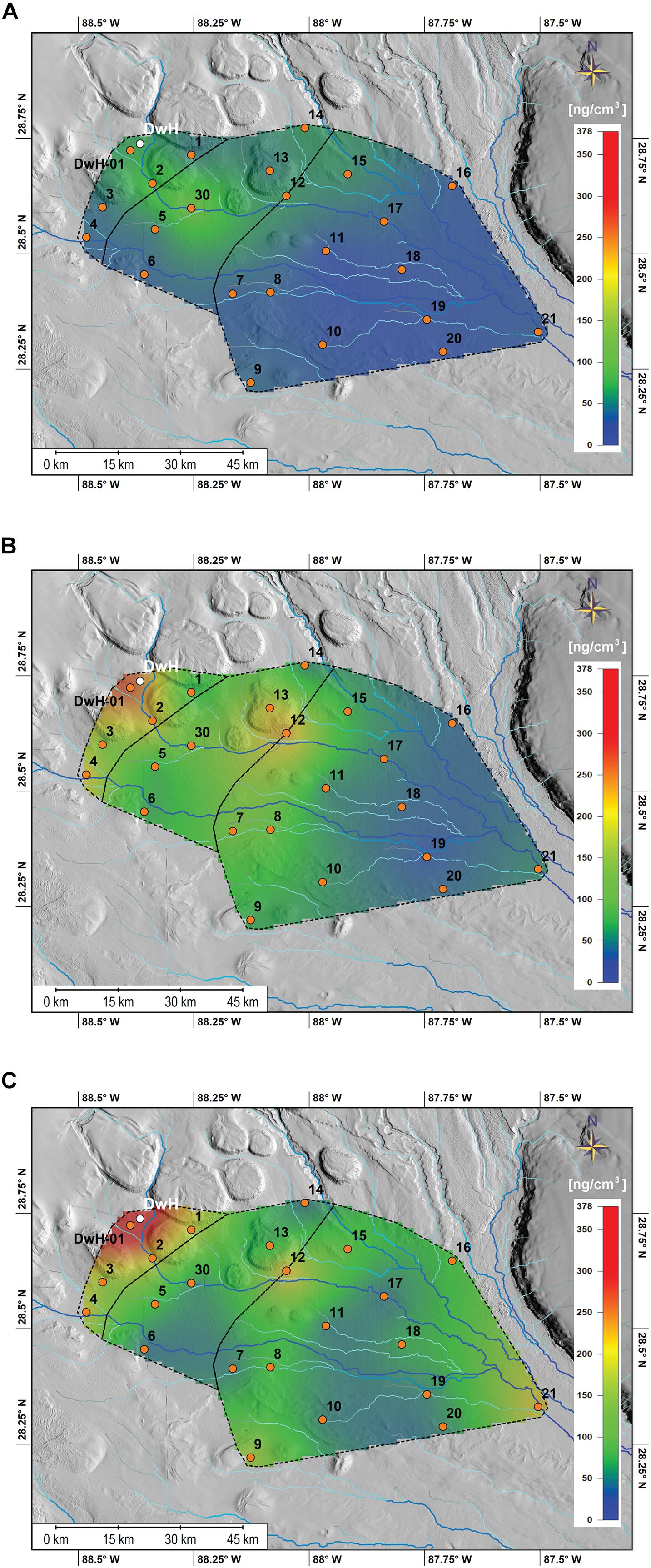
Figure 14. Sediment depth-integrated biomarker concentrations in deep-sea sediments by time periods: (A) prespill (<2010), (B) spill/post-spill (2010–2013), (C) post-spill (2014–2018). Biomarker concentrations include the sum of hopanes (C23–C35), steranes (C27–C29), triaromatic steroids (C20–C21, C26–C28). Time periods were determined based on the established chronology.

Conclusion

Overall, our results indicate an increased spatial footprint of deposition of DwH-derived hydrocarbons for which we offer two explanations. The deposition of contaminated sediments was not previously identified due to a lack of sampling in our study area and down-slope redistribution of sediments over the 8 years following the DwH oil spill and initial MOSSFA deposition to the seafloor. We based our conclusions on the characteristics of three regions as defined by their morphological and sedimentological features as well as the likelihood of sediments accumulating in these regions through episodic down-slope transport mechanisms. The nature of the organic compounds found in some of the cores, as well as sediment composition from these regions allowed us to trace them back to the DwH oil spill (in 15 out of 24 studied sites). Region 1 showed the presence of episodic sediment accumulation and had a potential for longer term accumulation and sequestration of redistributed sediments from up-slope areas. Region 2 was defined by stable and consistent sediment accumulation with low magnitude events in down-slope sediment accumulation being very subtle in the sedimentary record. We determined that this area is less likely to accumulate and sequester redistributed sediments. Region 3 had an increased presence of episodic sediment accumulation through larger magnitude pulse events. These events lead to a higher potential for accumulation and sequestration of redistributed sediments from up-slope areas.

Our findings presented in this paper, provide evidence that the footprint of the residues from the oil spill on the seafloor changed over the time span from 2010 to 2018 expanding to the SE beyond the previous areal extent reported. In the sedimentary record, DwH oil-residues were found in sites during the post-spill periods studied (2010–2013: during the MOSSFA event; 2014–2018: post MOSSFA event; sites: DwH-01, 2, 3, 4, 5, 6, 12, 13, 15, 30) as well as in sites only during the 2014–2018 period (sites: 1, 8, 21). Specifically, sites located approximately 45 km (site 8; 28.4166° N, 88.0838° W) and 96 km (site 21; 28.3306°N, 87.5042°W) to the SE of the wellhead, indicate a larger area affected by DwH oil residues due only to down slope redistribution of organic matter by natural process at depth in the GoM. Our data thus suggest that a much larger area on the seafloor contained residues of DWH oil than previously then previously recognized and published in the literature (Lehr et al., 2010; Chanton et al., 2012; Lubchenco et al., 2012; Romero et al., 2017).

Data Availability Statement

The datasets presented in this study can be found in online repositories. The names of the repository/repositories and accession number(s) can be found below: Data are publicly available through the Gulf of Mexico Research Initiative Information & Data Cooperative (GRIIDC) at https://data.gulfresearchinitiative.org: doi: 10.7266/n7-5xgs-mg78; doi: 10.7266/n7-ry85-yq61; 10.7266/n7-gzhr-0s83; doi: 10.7266/n7-zwvz-6a72; doi: 10.7266/n7-h6gj-1m18; doi: 10.7266/n7-391g-9t63; doi: 10.7266/N7445K2V; doi: 10.7266/n7-6bfd-g305; and doi: 10.7266/HCKBSN5J.

Author Contributions

All authors listed have made a substantial, direct and intellectual contribution to the work, and approved it for publication.

Funding

The REDIRECT (Resuspension, Redistribution and Deposition of Deepwater Horizon recalcitrant hydrocarbons to offshore depocenter) research was made possible by a grant from The Gulf of Mexico Research Initiative (GOMRI). Also, research was supported by an Early-Career Research Fellowship from the Gulf Research Program of the National Academies of Sciences, Engineering, and Medicine to IC Romero (Grant #2000010685). The content in this publication is solely the responsibility of the authors and does not necessarily represent the official views of the Gulf Research Program of the National Academies of Sciences, Engineering, and Medicine.

Conflict of Interest

The authors declare that the research was conducted in the absence of any commercial or financial relationships that could be construed as a potential conflict of interest.

Acknowledgments

The authors would like to thank the crew of the R/V Point Sur for their help during the field program and the technicians Hannah Hamontree, and Olivia Traenkle for laboratory support during chemical analyses of hydrocarbons.

Supplementary Material

The Supplementary Material for this article can be found online at: https://www.frontiersin.org/articles/10.3389/fmars.2021.630183/full#supplementary-material

References

Adhikari, P., Wong, R., and Overton, E. (2017). Application of enhanced gas chromatography/triple quadrupole mass spectrometry for monitoring petroleum weathering and forensic source fingerprinting in samples impacted by the deepwater horizon oil spill. Chemosphere 184, 939–950. doi: 10.1016/j.chemosphere.2017.06.077

PubMed Abstract | CrossRef Full Text | Google Scholar

Aeppli, C., Nelson, R. K., Radović, J. R., Carmichael, C. A., Valentine, D. L., and Reddy, C. M. (2014). Recalcitrance and degradation of petroleum biomarkers upon abiotic and biotic natural weathering of Deepwater Horizon oil. Environ. Sci. Technol. 48, 6726–6734. doi: 10.1021/es500825q

PubMed Abstract | CrossRef Full Text | Google Scholar

Appleby, P. G. (2001). “Chronostratigraphic techniques in recent sediments,” in Tracking Environmental Change Using Lake Sediments: Basin Analysis, Coring, and Chronological Techniques Developments in Paleoenvironmental Research, eds W. M. Last and J. P. Smol (Dordrecht: Springer Netherlands), 171–203. doi: 10.1007/0-306-47669-x_9

CrossRef Full Text | Google Scholar

Appleby, P. G., and Oldfield, F. (1983). The assessment of 210Pb data from sites with varying sediment accumulation rates. Hydrobiologia 103, 29–35. doi: 10.1007/BF00028424

CrossRef Full Text | Google Scholar

Ash-Mor, A., Bookman, R., Kanari, M., Ben-Avraham, Z., and Almogi-Labin, A. (2017). Micropaleontological and taphonomic characteristics of mass transport deposits in the northern Gulf of Eilat/Aqaba, Red Sea. Mar. Geol. 391, 36–47. doi: 10.1016/j.margeo.2017.07.009

CrossRef Full Text | Google Scholar

Baskaran, M., Nix, J., Kuyper, C., and Karunakara, N. (2014). Problems with the dating of sediment core using excess (210)Pb in a freshwater system impacted by large scale watershed changes. J. Environ. Radioact. 138, 355–363. doi: 10.1016/j.jenvrad.2014.07.006

PubMed Abstract | CrossRef Full Text | Google Scholar

Beaulieu, S. E. (2003). Resuspension of phytodetritus from the sea floor: a laboratory flume study. Limnol. Oceanogr. 48, 1235–1244. doi: 10.4319/lo.2003.48.3.1235

CrossRef Full Text | Google Scholar

Bejarano, A. C., and Michel, J. (2010). Large-scale risk assessment of polycyclic aromatic hydrocarbons in shoreline sediments from Saudi Arabia: environmental legacy after twelve years of the Gulf war oil spill. Environ. Pollut. 158, 1561–1569. doi: 10.1016/j.envpol.2009.12.019

PubMed Abstract | CrossRef Full Text | Google Scholar

Binford, M. W. (1990). Calculation and uncertainty analysis of 210Pb dates for PIRLA project lake sediment cores. J. Paleolimnol. 3, 253–267. doi: 10.1007/BF00219461

CrossRef Full Text | Google Scholar

Borrowman, T. D., Smith, E. R., Gailani, J. A., and Caviness, L. (2006). Erodibility Study of Passaic River Sediments Using USACE Sedflume. Fort Belvoir, VA: Defense Technical Information Center.

Google Scholar

Brady, H. B. (1878). On the reticularian and radiolarian rhizopoda (Foraminifera and Polycystina) of the North Polar Expedition of 1875-76. Ann. Mag. Nat. Hist. 5, 425–440. doi: 10.1080/00222937808682361

CrossRef Full Text | Google Scholar

Brady, H. B. (1879). Notes on some of the reticularian Rhizopoda of the challenger expedition, part i. on new or little known arenaceous types. Q. J. Microsc. Sci. 19, 20–63. doi: 10.1242/jcs.s2-19.73.20

CrossRef Full Text | Google Scholar

Brady, H. B. (1884). Report on the foraminifera dredged by H.M.S. Challenger during the years 1873-1876. Zoology 9, 1–814.

Google Scholar

Brooks, G. R., Larson, R. A., Schwing, P. T., Romero, I., Moore, C., Reichart, G.-J., et al. (2015). Sedimentation pulse in the NE gulf of mexico following the 2010 DWH Blowout. PLoS One 10:e0132341. doi: 10.1371/journal.pone.0132341

PubMed Abstract | CrossRef Full Text | Google Scholar

Camilli, R., Reddy, C. M., Yoerger, D. R., Van Mooy, B. A. S., Jakuba, M. V., Kinsey, J. C., et al. (2010). Tracking hydrocarbon plume transport and biodegradation at deepwater horizon. Science 330, 201–204. doi: 10.1126/science.1195223

PubMed Abstract | CrossRef Full Text | Google Scholar

Chanton, J. P., Cherrier, J., Wilson, R. M., Sarkodee-Adoo, J., Bosman, S., Mickle, A., et al. (2012). Radiocarbon evidence that carbon from the Deepwater Horizon spill entered the planktonic food web of the Gulf of Mexico. Environ. Res. Lett. 7:045303. doi: 10.1088/1748-9326/7/4/045303

CrossRef Full Text | Google Scholar

Chanton, J., Zhao, T., Rosenheim, B. E., Joye, S., Bosman, S., Brunner, C., et al. (2015). Using natural abundance radiocarbon to trace the flux of petrocarbon to the seafloor following the deepwater horizon oil spill. Environ. Sci. Technol. 49, 847–854. doi: 10.1021/es5046524

PubMed Abstract | CrossRef Full Text | Google Scholar

Choi, M., Kim, Y.-J., Lee, I.-S., and Choi, H.-G. (2014). Development of a one-step integrated pressurized liquid extraction and cleanup method for determining polycyclic aromatic hydrocarbons in marine sediments. J. Chromatogr. A 1340, 8–14. doi: 10.1016/j.chroma.2014.03.015

PubMed Abstract | CrossRef Full Text | Google Scholar

Choi, Y., and Wang, Y. (2004). Dynamics of carbon sequestration in a coastal wetland using radiocarbon measurements. Glob. Biogeochem. Cycles 18:GB4016. doi: 10.1029/2004GB002261

CrossRef Full Text | Google Scholar

Coleman, J. M., Bouma, A. H., Roberts, H. H., and Thayer, P. A. (1986). “Stratification in mississippi fan cores revealed by X-Ray radiography,” in Initial Reports of the Deep Sea Drilling Project, Vol. 96, eds A. H. Bouma, J. M. Coleman, and A. W. Meyer (Washington, D.C: U.S. Government Printing Office), 505–518.

Google Scholar

Cremer, M., and Stow, D. A. V. (1986). Sedimentary structures of fine-grained sediments from the Mississippi Fan: Thin Section Analysis. Initial Reports of the Deep Sea Drilling Project. XCVI., 96, 519–532. http://deepseadrilling.org/96/volume/dsdp96_24.pdf

Google Scholar

Crowsey, R. C. (2013). Persistence of gulf of mexico surface oil from the 2010 deepwater horizon spill. Southeast. Geogr. 53, 359–361. doi: 10.1353/sgo.2013.0034

CrossRef Full Text | Google Scholar

Cushman, J. A. (1922). Shallow-Water Foraminifera of the Tortugas Region. Carnegie Inst. Wash. 17, 1–85.

Google Scholar

Cushman, J. A. (1923). The foraminifera of the Atlantic Ocean. Part 4. Lagenidae. Bull. U.S. Natl. Mus. 104, 1–228. doi: 10.2113/49.suppl_2.1

CrossRef Full Text | Google Scholar

Cushman, J. A. (1927). New and interesting foraminifera from Mexico and Texas. Contributions Cushman Lab. Foraminifer. Res. 3, 111–117.

Google Scholar

d’Orbigny, A. D. (1826). Tableau méthodique de la classe des Céphalopodes. Ann. Sci. Nat. 7, 245–314.

Google Scholar

d’Orbigny, A. D. (1839). Voyage dans l’Amerique Meridionale. Paris and Strasbourg: Bertrand, 1–86.

Google Scholar

Daly, K. L., Passow, U., Chanton, J., and Hollander, D. (2016). Assessing the impacts of oil-associated marine snow formation and sedimentation during and after the Deepwater Horizon oil spill. Anthropocene 13, 18–33. doi: 10.1016/j.ancene.2016.01.006

CrossRef Full Text | Google Scholar

Daly, K. L., Vaz, A. C., and Paris, C. B. B. (2020). The Sedimentation and Lateral Transport of Oil-Associated Marine Snow During and After the Deepwater Horizon Oil Spill. in (AGU). doi: 10.1007/978-3-030-12963-7_18

CrossRef Full Text | Google Scholar

Dean, W. E. (1974). Determination of carbonate and organic matter in calcareous sediments and sedimentary rocks by loss on ignition; comparison with other methods. J. Sediment. Res. 44, 242–248. doi: 10.1306/74D729D2-2B21-11D7-8648000102C1865D

CrossRef Full Text | Google Scholar

Diercks, A.-R., Dike, C., Asper, V. L., DiMarco, S. F., Chanton, J. P., and Passow, U. (2018). Scales of seafloor sediment resuspension in the northern Gulf of Mexico. Elem. Sci. Anth. 6:32. doi: 10.1525/elementa.285

PubMed Abstract | CrossRef Full Text | Google Scholar

Diercks, A.-R., Highsmith, R. C., Asper, V. L., Joung, D., Zhou, Z., Guo, L., et al. (2010). Characterization of subsurface polycyclic aromatic hydrocarbons at the Deepwater Horizon site. Geophys. Res. Lett. 37:L20602. doi: 10.1029/2010GL045046

CrossRef Full Text | Google Scholar

Folk, R. L. (1965). Petrology of Sedimentary Rocks. Austin, TX: Hemphill.

Google Scholar

Gardner, W. D., and Sullivan, L. G. (1981). Benthic storms: temporal variability in a deep-ocean nepheloid layer. Science 213, 329–331. doi: 10.1126/science.213.4505.329

PubMed Abstract | CrossRef Full Text | Google Scholar

Gardner, W. D., Tucholke, B. E., Richardson, M. J., and Biscaye, P. E. (2017). Benthic storms, nepheloid layers, and linkage with upper ocean dynamics in the western North Atlantic. Mar. Geol. 385, 304–327. doi: 10.1016/j.margeo.2016.12.012

CrossRef Full Text | Google Scholar

Gros, J., Reddy, C. M., Aeppli, C., Nelson, R. K., Carmichael, C. A., and Arey, J. S. (2014). Resolving biodegradation patterns of persistent saturated hydrocarbons in weathered oil samples from the Deepwater Horizon disaster. Environ. Sci. Technol. 48, 1628–1637. doi: 10.1021/es4042836

PubMed Abstract | CrossRef Full Text | Google Scholar

Herrera-Herrera, A. V., Leierer, L., Jambrina-enríquez, M., Connolly, R., and Mallol, C. (2020). Evaluating different methods for calculating the Carbon Preference Index (CPI): implications for palaeoecological and archaeological research. Org. Geochem. 146:104056. doi: 10.1016/j.orggeochem.2020.104056

CrossRef Full Text | Google Scholar

Isley, A. E., Dale Pillsbury, R., and Laine, E. P. (1990). The genesis and character of benthic turbid events, Northern Hatteras Abyssal plain. Deep Sea Res. A Oceanogr. Res. Pap. 37, 1099–1119. doi: 10.1016/0198-0149(90)90053-X

CrossRef Full Text | Google Scholar

Jernelöv, A., and Lindén, O. (1981). Ixtoc I: a case study of the world’s largest oil spill. Ambio 10:299.

Google Scholar

Jones, J. P., and Parker, W. K. (1860). On the rhizopodal fauna of the mediterranean compared with that of the Italian and some other tertiary deposits. Q. J. Geol. Soc. Lond. 16, 292–307. doi: 10.1144/gsl.jgs.1860.016.01-02.41

CrossRef Full Text | Google Scholar

Joye, S. B., Crespo-Medina, M., Hunter, K., Asper, V., Diercks, A., Passow, U., et al. (2013). Increased sedimentation and altered nutrient cycling in the aftermath of the Macondo oil well blowout. Abstr. Pap. Am. Chem. Soc. 245.

Google Scholar

Kim, J. H., Moon, J. K., Li, Q. X., and Cho, J. Y. (2003). One-step pressurized liquid extraction method for the analysis of polycyclic aromatic hydrocarbons. Anal. Chim. Acta 498, 55–60. doi: 10.1016/j.aca.2003.08.049

CrossRef Full Text | Google Scholar

Kitto, M. E. (1991). Determination of photon self-absorption corrections for soil samples. Int. J. Radiat. Appl. Instrum. A 42, 835–839. doi: 10.1016/0883-2889(91)90221-L

CrossRef Full Text | Google Scholar

Kramer, K. V., and Shedd, B. (2017). A 1.4-Billion-Pixel Map of the Gulf of Mexico Seafloor. Eos. Available online at: https://eos.org/project-updates/a-1-4-billion-pixel-map-of-the-gulf-of-mexico-seafloor (Accessed January 11, 2018).

Google Scholar

Lampitt, R. S. (1985). Evidence for the seasonal deposition of detritus to the deep-sea floor and its subsequent resuspension. Deep Sea Res. A Oceanogr. Res. Pap. 32, 885–897. doi: 10.1016/0198-0149(85)90034-2

CrossRef Full Text | Google Scholar

Larson, R. A., Brooks, G. R., Schwing, P. T., Holmes, C. W., Carter, S. R., and Hollander, D. J. (2018). High-resolution investigation of event driven sedimentation: Northeastern Gulf of Mexico. Anthropocene 24, 40–50. doi: 10.1016/j.ancene.2018.11.002

CrossRef Full Text | Google Scholar

Lehr, B., Bristol, S., and Possolo, A. (2010). Oil Budget Calculator - Deepwater Horizon, A Report to the National Incident Command. https://www.restorethegulf.gov/sites/default/files/documents/pdf/OilBudgetCalc_Full_HQ-Print_111110.pdf

Google Scholar

Long, E. R., Macdonald, D. D., Smith, S. L., and Calder, F. D. (1995). Incidence of adverse biological effects within ranges of chemical concentrations in marine and estuarine sediments. Environ. Manag. 19, 81–97. doi: 10.1007/BF02472006

CrossRef Full Text | Google Scholar

Lubchenco, J., McNutt, M. K., Dreyfus, G., Murawski, S. A., Kennedy, D. M., Anastas, P. T., et al. (2012). Science in support of the Deepwater Horizon response. Proc. Natl. Acad. Sci. U.S.A. 109, 20212–20221. doi: 10.1073/pnas.1204729109

PubMed Abstract | CrossRef Full Text | Google Scholar

Meyer, B. M., Adhikari, P. L., Olson, G. M., Overton, E. B., and Miles, M. S. (2017). Louisiana Coastal Marsh Environments and MC252 Oil Biomarker Chemistry. Amsterdam: Elsevier Inc.

Google Scholar

Milliman, J. D. (1974). Marine carbonates. recent sedimentary carbonates part 1. Springer-Verlag, New York, Heidelberg, & Berlin, xv + 375 p. $25.50. Limno. Oceanogr. 19:876. doi: 10.4319/lo.1974.19.5.0876b

CrossRef Full Text | Google Scholar

Mulabagal, V., Yin, F., John, G. F., Hayworth, J. S., and Clement, T. P. (2013). Chemical fingerprinting of petroleum biomarkers in Deepwater Horizon oil spill samples collected from Alabama shoreline. Mar Pollut Bull 70, 147–154. doi: 10.1016/j.marpolbul.2013.02.026

PubMed Abstract | CrossRef Full Text | Google Scholar

Normark, W. R., Meyer, A. W., Cremer, M., Droz, L., O’Connell, S., Pickering, K. T., et al. (1986). “Summary of drilling results for the Mississippi Fan and considerations for applications to other turbidite systems,” in Initial Reports of the Deep Sea Drilling Project, eds A. H. Bouma, J. M. Coleman, and A. W. Meyer (Washington, DC: U.S. Government Printing Office), 425–436.

Google Scholar

Osterman, L. E. (2003). Benthic foraminifers from the continental shelf and slope of the Gulf of Mexico: an indicator of shelf hypoxia. Estuar. Coast. Shelf Sci. 58, 17–35. doi: 10.1016/S0272-7714(02)00352-9

CrossRef Full Text | Google Scholar

Parker, F. L. (1954). Distribution of foraminifera in the Northeastern Gulf of Mexico. Bull. Mus. Comp. Zool. 111, 453–588.

Google Scholar

Parker, F. L., Phleger, F. B., and Pierson, J. F. (1953). North Atlantic foraminifera. Rep. Swedish Deep Sea Expedition, 1947-1948 7, 3–122.

Google Scholar

Parker, W. K., and Jones, T. R. (1865). On some foraminifera from the coast of Norway. Ann. Mag. Nat. Hist. 155, 325–441.

Google Scholar

Passow, U., Chanton, J. P., Hollander, D., and Dahly, K. (2013). MOSSFA (Marine Oil Snow Sedimentation and Flocculent Accumulation) Working Group. Tallahassee, FL: Florida State University.

Google Scholar

Passow, U., Ziervogel, K., Asper, V., and Diercks, A. (2012). Marine snow formation in the aftermath of the deepwater horizon oil spill in the Gulf of Mexico. Environ. Res. Lett. 7:035301. doi: 10.1088/1748-9326/7/3/035301

CrossRef Full Text | Google Scholar

Patterson, R. T., and Fishbein, E. (1989). Re-examination of the statistical methods used to determine the number of point counts needed for micropaleontological quantitative research. J. Paleontol. 63, 245–248. doi: 10.1017/S0022336000019272

CrossRef Full Text | Google Scholar

Phleger, F. B., and Parker, F. L. (1951). Gulf of mexico foraminifera, Part 1 and 2. Geol. Soc. Am. Mem. 46.

Google Scholar

Prince, R. C., Owens, E. H., and Sergy, G. A. (2002). Weathering of an Arctic oil spill over 20 years: the BIOS experiment revisited. Mar. Pollut. Bull. 44, 1236–1242. doi: 10.1016/s0025-326x(02)00214-x

CrossRef Full Text | Google Scholar

Ramdahl, T. (1983). Retene–a molecular marker of wood combustion in ambient air. Nature 306, 580–582. https://doi.org/10.1038/306580a0

Google Scholar

Romero, I. C., Chanton, J. P., Brooks, J. R., Bosman, S., Larson, R. A., Harris, A., et al. (2021). Molecular markers of biogenic and oil-derived hydrocarbons in deep-sea sediments following the Deepwater Horizon spill. Front. Mar. Sci. (in press). doi: 10.3389/fmars.2021.637970

CrossRef Full Text | Google Scholar

Romero, I. C., Schwing, P. T., Brooks, G. R., Larson, R. A., Hastings, D. W., Ellis, G., et al. (2015). Hydrocarbons in deep-sea sediments following the 2010 deepwater horizon blowout in the Northeast Gulf of Mexico. PLoS One 10:e0128371. doi: 10.1371/journal.pone.0128371

PubMed Abstract | CrossRef Full Text | Google Scholar

Romero, I. C., Sutton, T., Carr, B., Quintana-Rizzo, E., Ross, S. W., Hollander, D. J., et al. (2018). Decadal Assessment of polycyclic aromatic hydrocarbons in mesopelagic fishes from the gulf of mexico reveals exposure to oil-derived sources. Environ. Sci. Technol. 52, 10985–10996. doi: 10.1021/acs.est.8b02243

PubMed Abstract | CrossRef Full Text | Google Scholar

Romero, I. C., Toro-Farmer, G., Diercks, A.-R., Schwing, P., Muller-Karger, F., Murawski, S., et al. (2017). Large-scale deposition of weathered oil in the Gulf of Mexico following a deep-water oil spill. Environ. Pollut. 228, 179–189. doi: 10.1016/j.envpol.2017.05.019

PubMed Abstract | CrossRef Full Text | Google Scholar

Schwing, P. T., Brooks, G. R., Larson, R. A., Holmes, C. W., O’Malley, B. J., and Hollander, D. J. (2017). Constraining the spatial extent of marine oil snow sedimentation and flocculent accumulation following the deepwater horizon event using an excess 210 Pb flux approach. Environ. Sci. Technol. 51, 5962–5968. doi: 10.1021/acs.est.7b00450

PubMed Abstract | CrossRef Full Text | Google Scholar

Schwing, P. T., O’Malley, B. J., and Hollander, D. J. (2018). Resilience of benthic foraminifera in the Northern Gulf of Mexico following the Deepwater Horizon event (2011–2015). Ecol. Indic. 84, 753–764. doi: 10.1016/j.ecolind.2017.09.044

CrossRef Full Text | Google Scholar

Schwing, P. T., Romero, I. C., Larson, R. A., O’Malley, B. J., Fridrik, E. E., Goddard, E. A., et al. (2016). Sediment core extrusion method at millimeter resolution using a calibrated, threaded-rod. J. Vis. Exp. 114, 54363. doi: 10.3791/54363

PubMed Abstract | CrossRef Full Text | Google Scholar

Smith, L. M., Alexander, C., and Jennings, A. E. (2002). Accumulation in east greenland fjords and on the continental shelves adjacent to the denmark strait over the last century based on 210Pb geochronology. ARCTIC 55, 109–122. doi: 10.14430/arctic695

CrossRef Full Text | Google Scholar

Sørensen, L., Meier, S., and Mjøs, S. A. (2016). Application of gas chromatography/tandem mass spectrometry to determine a wide range of petrogenic alkylated polycyclic aromatic hydrocarbons in biotic samples. Rapid Commun. Mass Spectrom. 30, 2052–2058. doi: 10.1002/rcm.7688

PubMed Abstract | CrossRef Full Text | Google Scholar

Stewart, R. E., and Stewart, K. C. (1930). Post-miocene foraminifera from the ventura quadrangle, ventura county, California. J. Paleontol. 4, 60–72.

Google Scholar

Stout, S. A., Payne, J. R., Ricker, R. W., Baker, G., and Lewis, C. (2016). Macondo oil in deep-sea sediments: part 2 — distribution and distinction from background and natural oil seeps. Mar. Pollut. Bull. 111, 381–401. doi: 10.1016/j.marpolbul.2016.07.041

PubMed Abstract | CrossRef Full Text | Google Scholar

Stow, D. A. V., Cremer, M., Droz, L., Meyer, A. W., Normark, W. R., O’Connell, S., et al. (1986). “Facies, composition, and texture of Mississippi Fan sediments, Deep Sea Drilling Project Leg 96, Gulf of Mexico,” in Initial Reports of the Deep Sea Drilling Project, eds A. H. Bouma, J. M. Coleman, and A. W. Meyer (Washington, DC: U.S. Government Printing Office), 475–488.

Google Scholar

Stuiver, M., and Polach, H. A. (1977). Discussion reporting of 14 C Data. Radiocarbon 19, 355–363. doi: 10.1017/S0033822200003672

CrossRef Full Text | Google Scholar

Swarzenski, P. W. (2014). “210Pb dating,” in Encyclopedia of scientific dating methods, eds W. J. Rink and J. Thompson (Dordrecht: Springer Netherlands), 1–11. doi: 10.1007/978-94-007-6326-5_236-1

CrossRef Full Text | Google Scholar

Thayer, P., Roberts, H. H., Bouma, A. H., and Coleman, J. M. (1986). “Sedimentology and petrology of mississippi fan depositional environments, deep sea drilling project leg 96,” in Initial Reports of the Deep Sea Drilling Project, eds A. H. Bouma, J. M. Coleman, and A. W. Meyer (Washington, D.C: U.S. Government Printing Office), 489–504.

Google Scholar

Tobiszewski, M., and Namieśnik, J. (2012). PAH diagnostic ratios for the identification of pollution emission sources. Environ. Pollut. 162, 110–119. doi: 10.1016/j.envpol.2011.10.02

CrossRef Full Text | Google Scholar

Turnewitsch, R., Dale, A., Lahajnar, N., Lampitt, R. S., and Sakamoto, K. (2017). Can neap-spring tidal cycles modulate biogeochemical fluxes in the abyssal near-seafloor water column? Prog. Oceanogr. 154, 1–24. doi: 10.1016/j.pocean.2017.04.006

CrossRef Full Text | Google Scholar

Turnewitsch, R., Falahat, S., Nycander, J., Dale, A., Scott, R. B., and Furnival, D. (2013). Deep-sea fluid and sediment dynamics—influence of hill- to seamount-scale seafloor topography. Earth Sci. Rev. 127, 203–241. doi: 10.1016/j.earscirev.2013.10.005

CrossRef Full Text | Google Scholar

Turnewitsch, R., Reyss, J.-L., Chapman, D. C., Thomson, J., and Lampitt, R. S. (2004). Evidence for a sedimentary fingerprint of an asymmetric flow field surrounding a short seamount. Earth Planet. Sci. Lett. 222, 1023–1036. doi: 10.1016/j.epsl.2004.03.042

CrossRef Full Text | Google Scholar

Valentine, D. L., Fisher, G. B., Bagby, S. C., Nelson, R. K., Reddy, C. M., Sylva, S. P., et al. (2014). Fallout plume of submerged oil from Deepwater Horizon. Proc. Natl. Acad. Sci. U.S.A. 111, 15906–15911. doi: 10.1073/pnas.1414873111

PubMed Abstract | CrossRef Full Text | Google Scholar

Vogel, J. S., Southon, J. R., Nelson, D. E., and Brown, T. A. (1984). Performance of catalytically condensed carbon for use in accelerator mass spectrometry. Nuclear Instruments and Methods in Physics Research Section B: Beam Interactions with Materials and Atoms, 5, 289–293. https://doi.org/10.1016/0168-583X(84)90529-9

Google Scholar

Wang, Z., and Fingas M. F. (2003). Development of oil hydrocarbon fingerprinting and identification techniques. Mar Pollut Bull 47, 423–452. doi: 10.1016/S0025-326X(03)00215-7

CrossRef Full Text | Google Scholar

Wang, Z., Fingas, M., Shu, Y. Y., Sigouin, L., Landriault, M., Lambert, P., et al. (1999). Quantitative Characterization of PAHs in Burn Residue and Soot Samples and Differentiation of Pyrogenic PAHs from Petrogenic PAHs-The 1994 Mobile Burn Study. Environ. Sci. Technol. 33, 3100–3109. doi: 10.1021/es990031y

CrossRef Full Text | Google Scholar

Wang, Z., Stout, S. A., and Fingas, M. (2006). Forensic Fingerprinting of Biomarkers for Oil Spill Characterization and Source Identification. Environ. Forensics 7, 105–146. doi: 10.1080/15275920600667104

CrossRef Full Text | Google Scholar

Wang, Z. D., Fingas, M., Owens, E. H., Sigouin, L., and Brown, C. E. (2001). Long-term fate and persistence of the spilled Metula oil in a marine salt marsh environment - degradation of petroleum biomarkers. J. Chromatogr. A 926, 275–290. doi: 10.1016/s0021-9673(01)01051-2

CrossRef Full Text | Google Scholar

White, H. K., Wang, C. H., Williams, P. L., Findley, D. M., Thurston, A. M., Simister, R. L., et al. (2016). Long-term weathering and continued oxidation of oil residues from the Deepwater Horizon spill. Mar. Pollut. Bull. 113, 380–386. doi: 10.1016/j.marpolbul.2016.10.02

CrossRef Full Text | Google Scholar

Williamson, W. C. (1858). On the Recent Foraminifera of Great Britain. Ray Society, 1–107. doi: 10.5962/bhl.title.139719

CrossRef Full Text | Google Scholar

Xing, L., Zhang, H., Yuan, Z., Sun, Y., and Zhao, M. (2011). Terrestrial and marine biomarker estimates of organic matter sources and distributions in surface sediments from the East China Sea shelf. Cont. Shelf Res. 31, 1106–1115. doi: 10.1016/j.csr.2011.04.003

CrossRef Full Text | Google Scholar

Yan, B., Passow, U., Chanton, J. P., Nöthig, E.-M., Asper, V., Sweet, J., et al. (2016). Sustained deposition of contaminants from the Deepwater Horizon spill. Proc. Natl. Acad. Sci. U.S.A. 113, E3332–E3340. doi: 10.1073/pnas.1513156113

PubMed Abstract | CrossRef Full Text | Google Scholar

Ziervogel, K., Dike, C., Asper, V., Montoya, J., Battles, J., D×souza, N., et al. (2016). Enhanced particle fluxes and heterotrophic bacterial activities in Gulf of Mexico bottom waters following storm-induced sediment resuspension. Deep Sea Res. II Top. Stud. Oceanogr. 129, 77–88. doi: 10.1016/j.dsr2.2015.06.017

CrossRef Full Text | Google Scholar