Assessing Habitat Suitability Models for the Deep Sea: Is Our Ability to Predict the Distributions of Seafloor Fauna Improving?

Introduction

Understanding and managing ecosystem effects of human activities, such as bottom-contact fishing and mineral extraction in the deep sea (depths greater than ca. 200 m), requires quantitative information on the distributions of benthic habitats and fauna (Kaiser et al., 2016; Pitcher et al., 2017). Because such information is generally sparse in waters beyond coastal areas, management decision-making relies increasingly on outputs from habitat suitability models (also known as species distribution models), which develop correlations between point-sampled faunal occurrence records and spatially continuous environmental variables to predict probabilities of suitable habitat or taxon occurrence across unsampled environmental space (Guisan and Zimmermann, 2000; Elith and Leathwick, 2009; Guisan et al., 2013; Vierod et al., 2014; Reiss et al., 2015). Methods commonly in use include Boosted Regression Trees (BRT, Friedman et al., 2000; Leathwick et al., 2006; De’ath, 2007), Generalized Additive Models (GAM), Maximum Entropy (MaxEnt, Phillips et al., 2006), and Random Forests (RF, Breiman, 2001). These and other types of habitat suitability models are in constant development (e.g., Warton et al., 2015) and are used increasingly in a broad range of applications (Guisan et al., 2013; Robinson et al., 2017; Araujo et al., 2019). The fundamental requirements of all methods, however, are the same: accurate and sufficient point-sample data about where a taxon has been recorded and, ideally, where it is has been confirmed to be absent, and accurate and ecologically relevant environmental data as continuous layers spanning the region of interest.

The relative paucity, patchiness, and taxonomic selectivity of available faunal sample data in the deep sea, a lack of spatial resolution and local validation of environmental layers, and limited understanding of biotic interactions and historical factors that might influence present distributions, in combination, can result in high levels of uncertainty being associated with the outputs from habitat suitability models (Fielding and Bell, 1997; Araujo and Guisan, 2006; Vierod et al., 2014; Reiss et al., 2015; Anderson et al., 2016a). This uncertainty is exacerbated by the cross-validation methods commonly used to evaluate model performance, in which subsets of the input taxon occurrence data are withheld from the model and used as test sites to assess predictions. While this approach is practical, it can generate overly optimistic values of model performance (Bahn and Mcgill, 2013; Ploton et al., 2020) that may not be supported by field validation (Anderson et al., 2016a) because the data used in cross-validation methods are not independent from those used to build the model itself and are likely to be spatially biased (e.g., Lobo et al., 2008; Ploton et al., 2020).

Evaluation against data collected independently of those used in the modeling process is the most convincing approach to model assessment because it is directly relevant to the way in which model predictions are used in practice: if we are to have confidence in the model outputs, we need to know how reliable they are in relation to independent observations of the target taxa (Verbyla and Litvaitis, 1989; Fielding and Bell, 1997; Pearce and Ferrier, 2000; Araujo et al., 2019). An important point here is that such independent observations should be made using methods that detect the taxa of interest reliably. In most studies of benthic invertebrate taxa in the deep sea, taxon occurrence data are compiled from sampling methods, typically demersal fish trawls, that are not efficient at catching benthos, leading to unquantified uncertainty in relation to detection and selectivity. Evaluation against independent data is rare, however, for the same reasons that habitat suitability modeling itself is a useful tool. That is, sample data about species’ occurrences are usually sparse because such data are time-consuming, logistically challenging, and expensive to collect and habitat suitability modeling approaches have been developed as a more pragmatic, rapid, and affordable way to map distributions. However, because independent validation of models is rarely undertaken, confidence in their predictions can be low, limiting their credibility for use in environmental management (Anderson et al., 2016a; Winship et al., 2020). Model uncertainty can be reduced by development of more sophisticated modeling methods or by increasing the quality and quantity of data inputs but without evaluation of performance against independent data, we cannot be sure that such developments translate into practical gains. Therefore, in places where successive models have been developed, with progressive updates to input data and modeling techniques, it is important to understand whether more recent models represent improvements in terms of increased prediction accuracy and thereby build confidence in their use for fisheries and other management purposes.

In New Zealand and the wider southwest Pacific region, growing concern about the ecosystem effects of fisheries and potential seabed mineral extraction operations has stimulated interest in improving knowledge about the distributions of seafloor fauna (Rowden et al., 2019). Habitat suitability modeling has been used in several studies of seafloor faunal distributions, mostly for sessile invertebrate taxa such as corals and sponges that are recognized as being particularly sensitive or vulnerable to anthropogenic disturbances (e.g., Tracey et al., 2011; Anderson et al., 2014) but also for demersal fishes (Leathwick et al., 2006) and mobile benthic fauna (Compton et al., 2013; Bowden et al., 2019a). The potential of habitat suitability modeling methods to predict distributions across unsampled space is of particular appeal in the region because, despite being rich in biological and mineral resources, relatively little of its seafloor has been surveyed in detail, other than in areas of particular interest for fisheries research. Many of the broad-scale habitat suitability modeling initiatives in this region arose as direct or indirect consequences of concerns about the seabed impacts of commercial bottom-contact fisheries. Bottom trawl fisheries target hoki (Macruronus novaezelandiae) and other demersal species on smooth substrata over large areas of New Zealand’s Exclusive Economic Zone (EEZ) in depths of 300–1,400 m and deep-sea species including orange roughy (Hoplostethus atlanticus), oreo (Oreosomatidae), and alfonsino (primarily Beryx splendens) on seamounts and other underwater topographic features throughout the region (Fisheries New Zealand, 2020). Much of what is known about the distributions of non-target seafloor taxa comes from bycatch records from these fisheries and the research trawl surveys that inform catch advice for them (O’Driscoll et al., 2011), and most habitat suitability models in the region have been based on occurrence data from these records in combination with records from museum and other specimen collection databases.

The only evaluation of deep-sea habitat suitability model predictions using data collected independently and by methods designed to detect the target taxa to date in the region is the study of Anderson et al. (2016a), in which the authors of the present paper first developed models for cold-water coral taxa, then designed and ran a seabed photographic survey specifically to test their predictions on the Louisville Seamount Chain to the east of New Zealand. We found that the models performed poorly in practice and attributed this to a number of potential factors, including a lack of reliably supported taxon absence records, low precision of available environmental variables, particularly bathymetry, and lack of ecologically relevant variables, such as substrate type, which are key determinants of benthic taxon distributions. In light of these results and a general lack of confidence in modeled distributions for use in environmental management, Fisheries New Zealand and the National Institute of Water and Atmospheric Research initiated a project to independently assess the predictive performance of existing models and improve confidence in future predictions. Focusing on a major fisheries area in New Zealand, Chatham Rise, the first stage of this project was to generate a fully independent, quantitative, dataset of seabed faunal distributions derived from photographic surveys that would enable objective assessment of existing habitat suitability models for the region (Bowden et al., 2019b).

Here, we use this independent dataset to assess the usefulness of outputs from published habitat suitability models for the region. We first use best-practice model building standards proposed by Araujo et al. (2019) to rank the existing models in order of their expected predictive performance, then by comparing model predictions against the independent data, we generate five metrics describing performance: area under the receiver operating characteristic curve (AUC); true skill statistic (TSS); results from t-tests comparing the mean of published model probability values for all locations at which a taxon was present in the independent test data against the mean value for locations at which it was absent; and correlation strength between predicted probability of suitable habitat for a given taxon and both its prevalence in the test data (R²_prev) and its standardized population density in the test data (R²_dens). We use these metrics to assess how well each model performs in absolute terms, and to rank them in order of realized performance, which we hypothesize should match the expected ranking based on the Araujo et al. (2019) criteria. We then refer to the Araujo et al. (2019) criteria to discuss which aspects of model development have the greatest influence on realized model performance.

Materials and Methods

Study Area

The study focuses on Chatham Rise because this part of New Zealand’s EEZ has the highest density of seafloor photographic survey data available for use in model evaluation, is physically central to many of the habitat suitability models available for evaluation in the region, and is the source of much of the specimen data that informed development of these models (Figure 1). Chatham Rise is a continental rise that extends eastward from the South Island of New Zealand for approximately 1,000 km, with the Chatham Islands toward the eastern end. The Sub-Tropical Front coincides with and is partially constrained by the rise, making it the most biologically productive fisheries region in the EEZ (McClatchie et al., 1997; Clark et al., 2000; Marchal et al., 2009; Nodder et al., 2012). Recent summaries of bottom-contact trawl history across Chatham Rise (Black et al., 2013; Black and Tilney, 2015; Baird and Mules, 2019) show high trawling intensity, primarily from the hoki fishery, at a 450–700-m depth west of Mernoo Bank and on the southern and northern central flanks of Chatham Rise, with locally very high intensities of trawling for orange roughy, oreo, and alfonsino on seamount and knoll features on the northern, eastern, and southern flanks. At present, initiatives to protect benthic habitats and fauna are limited to closures to fishing on some seamounts in the “Graveyard” and “Andes” regions (since 2001) on the northwest and southeast flanks of the rise, respectively (Brodie and Clark, 2003; Clark and Dunn, 2012), and establishment in 2007 of two benthic protection areas (BPAs): the Mid Chatham Rise BPA and the East Chatham Rise BPA (Helson et al., 2010).

FIGURE 1

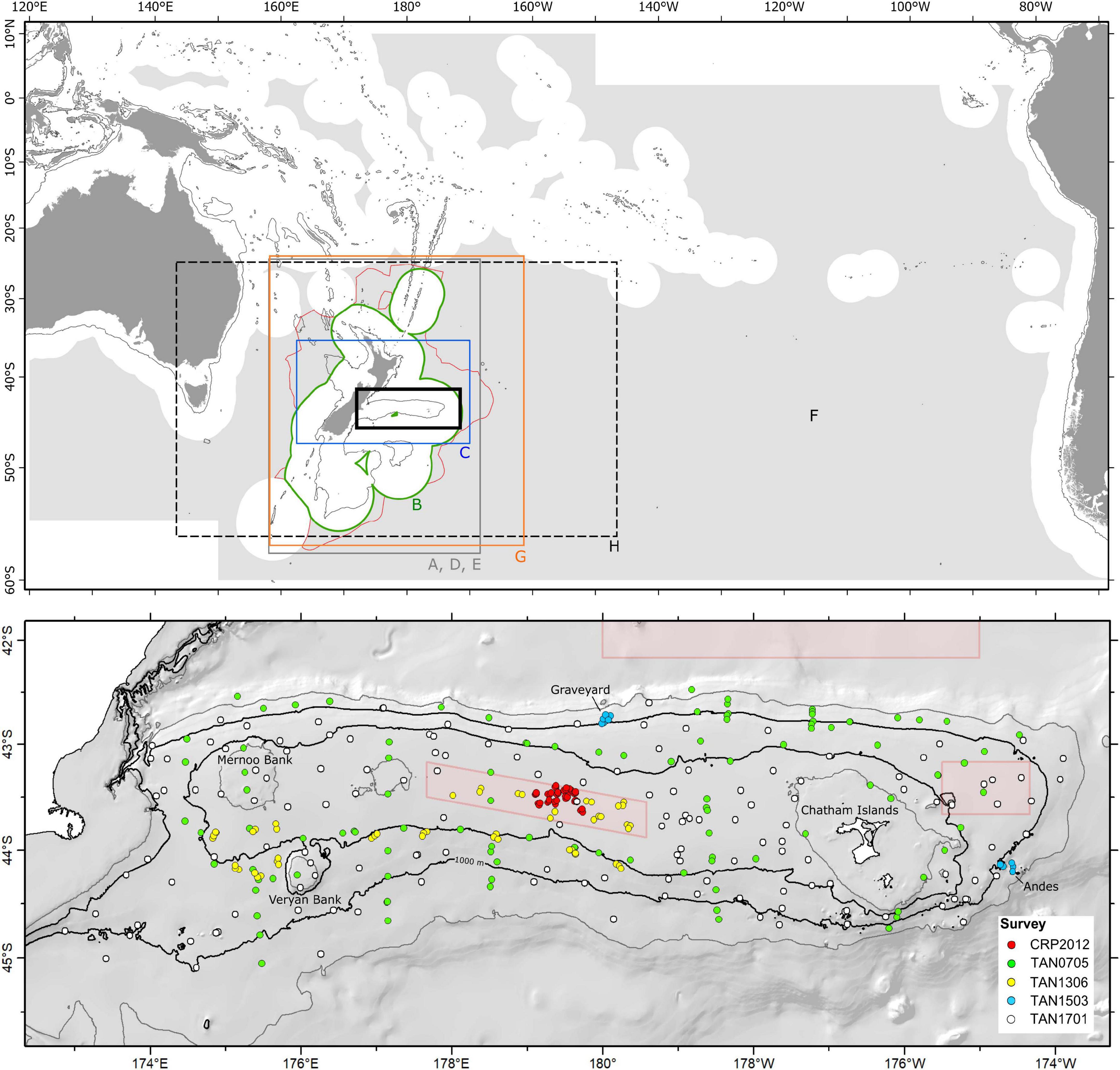
Figure 1. (Top) areas of eight published studies from which predictive models were assessed: A, Tracey et al. (2011); B, Baird et al. (2013); C, Compton et al. (2013); D, Anderson et al. (2014); E, Anderson et al. (2015); F, Anderson et al. (2016a), G, Anderson et al. (2016b); and H, Georgian et al. (2019). Boundary B is the New Zealand Exclusive Economic Zone (EEZ). Also showing New Zealand’s Extended Continental Shelf boundary (red polygon), the 1,000-m isobath, and Chatham Rise (bold black rectangle). (Bottom) Chatham Rise showing the location of DTIS photographic transect stations (color-coded points, see legend) for the five surveys from which the independent test dataset was developed. The Graveyard and Andes seamount complexes are indicated, isobaths show 250-, 500-, 1, 000-, and 1,500-m depths, and red polygons show Benthic Protection Areas (BPAs), which are protected from seabed trawl fishing.

Existing Models

Predictive models of habitat suitability for benthic epifaunal invertebrate taxa that encompass Chatham Rise have been published, primarily, in eight separate studies by our research team since 2011 (Tracey et al., 2011; Baird et al., 2013; Compton et al., 2013; Anderson et al., 2014, 2015, 2016a,b; Georgian et al., 2019). Most of these studies have focused on protected corals (Tracey et al., 2011; Baird et al., 2013; Anderson et al., 2014, 2015) and vulnerable marine ecosystem (VME, sensu FAO, 2009) indicator taxa (Anderson et al., 2016a,b; Georgian et al., 2019), with only one study producing models for individual species across a wide range of taxonomic groups (Compton et al., 2013). We selected models for taxa that were well represented in our independent dataset (see below), with presence records at nine or more sites within the spatial domain of the model. Across the eight studies, 47 individual models spanning 31 taxa (Table 1) were suitable for assessment against the independent dataset.

TABLE 1

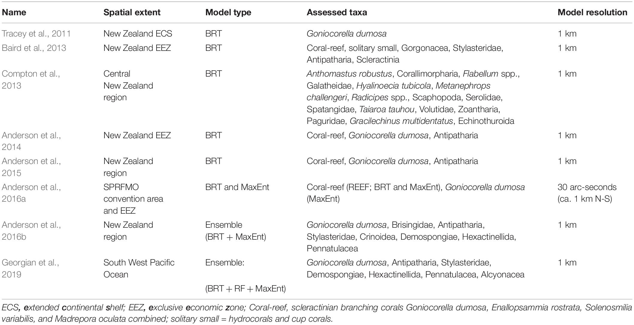
Table 1. Summary details of the eight existing SDM studies and the individual models suitable for assessment against the independent dataset.

All of the studies were undertaken with the principal aim of predicting occurrence across unsampled geographic space within the geographic range of their input faunal data (Prediction, sensu Araujo and Guisan, 2006; Araujo et al., 2019). Three modeling techniques were used across the studies: BRT, RF, and MaxEnt, with BRT being the most commonly used. The treatment of input data varied across studies, particularly in the approach to defining absence records. Five studies worked with presence–background data, using either randomly selected or spatially structured background points from the study area as assumed “pseudo-absences” (Tracey et al., 2011; Baird et al., 2013; Anderson et al., 2014, 2016a; Georgian et al., 2019), while the others used presence–absence data, deriving absence sites either from a combination of research trawl bycatch and museum databases or, in the case of Compton et al. (2013), from the source photographic survey data. Presence–absence models give an indication of the probability of a taxon being present, whereas models using pseudo-absences provide only a measure of the probability of suitable habitat being present.

The spatial extents of the studies range from the entire South Pacific Regional Fisheries Management Organisation (SPRFMO) Convention area (Anderson et al., 2016a) down to a section of the central part of the New Zealand EEZ (Compton et al., 2013), but all are centered on Chatham Rise (Figure 1). Spatial resolution for all studies was constrained to 1 km² by the resolution of available environmental predictor data. This resolution approximates to that of most of the methods used to collect the underlying sample data—primarily towed sampling gear including trawls, dredges, and epibenthic sleds—and matches closely the length of photographic transects from which the independent data were compiled.

All but one of the published studies were trained on benthic invertebrate sample data from physical specimens from research trawl surveys, fisheries bycatch, and museum collections, with most occurrence records coming from within the New Zealand EEZ, and many of these from Chatham Rise itself. Compton et al. (2013), by contrast, used observation data from photographic transects and epibenthic sled samples collected during two dedicated surveys of benthic biodiversity, one of which was TAN0705 (see below for relevance). All studies used k-fold cross-validation to evaluate model performance, a technique in which portions of the available sample data are iteratively withheld from the model training phase and then used to generate performance metrics based on how well the model predicts their values. The detail of how this validation was performed varied across studies, from random withholding of sites across the entire model domain (e.g., Tracey et al., 2011) to selection within longitudinal bands to compensate for spatial structuring of sample data (Anderson et al., 2016b). Spatial autocorrelation in the input sample data was addressed explicitly only in the most recent study (Georgian et al., 2019), by inclusion of a residual auto-covariate (RAC) predictor variable in their models (Crase et al., 2012). All of the studies used the area under the receiver-operating characteristic curve (AUC, Hanley and Mcneil, 1982; Swets, 1988; Bradley, 1997) as their metric of model predictive success.

Expected Performance

Before evaluating the published models against the independent dataset, we ranked the eight studies in order of their expected performance by applying the standards for best practice in habitat suitability modeling proposed by Araujo et al. (2019). The aim of this ranking was to place our results in the context of an objective framework that might subsequently help identify which aspects of the models contributed most to their predictive performance when assessed against independent data. The standards span the four broad components of model design: response variables, predictor variables, model building, and model evaluation, nested within which there are 15 “issues” (Table 2), each with guidelines allowing a given model to be ranked as either “Gold” (best practice), “Silver,” “Bronze,” or “Deficient.” Each author in the present paper scored each study for each of the 15 issues independently. Scores were then discussed, adjusted by consensus, and the studies ranked in order of overall score, with the expectation that models from higher-ranking studies should perform better against the independent data than those from lower-ranking ones.

TABLE 2

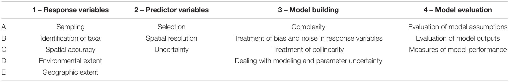
Table 2. Predictive model assessment criteria (1–4) and issues (A–E) proposed by Araujo et al. (2019).

Independent Dataset

Source Data

A dataset of benthic mega-epifauna density records from Chatham Rise was assembled from quantitative analyses of seabed video and still-image transects from five research surveys conducted between 2007 and 2017 (Figure 1). Voyages TAN0705 (Bowden, 2011; Compton et al., 2013), TAN1701 (Bowden et al., 2017), and TAN1306 (Bowden and Leduc, 2017) were broad-scale surveys of benthic biodiversity following stratified random designs, while voyage TAN1503 was focused on seamounts, with multiple summit-to-base camera transects on features in the Graveyard and Andes seamount complexes (Clark et al., 2019). Voyage CRP2012 (Rowden et al., 2014) focused on areas of phosphorite-rich sediments on the central crest area of Chatham Rise, using a design with replicate transects within multiple survey blocks. Data derived from these surveys are independent from those used to train the published models in that they were collected without reference to the original source data or the surveys from which they were compiled. They are, however, from a region of the published model domains that has the highest density of sample data and, thus, are spatially interspersed with the original training data.

Quantitative data on the occurrence of benthic invertebrate fauna were extracted from imagery from each survey under separate research projects over a period of 10 years (see survey references above), but the data extraction methods used were similar throughout, being run by the same team of researchers (DB, AR, and MC). These methods, and the auditing procedures that were used to create a combined dataset of faunal occurrences, are described in detail by Bowden et al. (2019b). In brief, seafloor photographic transects of approximately 1 km distance were run at each survey site, recording either high-definition digital color video (HD1080 format), digital still images (at 8-, 10-, 12-, or 24-megapixel resolution, depending on survey), or, for most surveys, both formats simultaneously. Four of the surveys used the same towed camera system (NIWA’s Deep Towed Imaging System, DTIS, Hill, 2009; Bowden and Jones, 2016), which records continuous HD video with intermittent high-resolution still images captured simultaneously at 15-s intervals and was deployed using the same operating procedures and methods for logging navigational and observational data on all surveys. The CRP2012 survey was conducted by remotely operated vehicle (ROV) on the central Chatham Rise crest. It was designed by the same research group (AR and DB) specifically to generate data compatible with standard DTIS surveys but the ROV used lower-resolution video and still-image cameras.

For surveys TAN0705, TAN1306, and TAN1701, the full length of each video transect was reviewed by analysts using Ocean Floor Observation Protocol (OFOP, Huetten and Greinert, 2008) software to record the occurrence and taxonomic identities of all fauna visible (larger than ca. 5 cm) on the seabed and referring to the high-resolution still images to confirm taxonomic identifications in consultation with taxonomic experts. In this method, each occurrence is referenced by spatial coordinates and time, enabling direct retrospective audit of individual records by examination of the original imagery. For surveys CRP2012 and TAN1503, still images were analyzed, rather than video; for the former because video quality was too low, and for the latter, to be comparable with data from earlier surveys (Clark et al., 2019). Merging data from the five surveys involved three stages: (1) checking and aligning taxon identities to ensure consistency of identifications and nomenclature; (2) comparing taxon presence and counts in areas of survey overlap to check for systematic survey or analyst bias; and (3) aggregating taxa into higher groupings where necessary to match those used in the nine published models under evaluation. For example, several of the modeling studies produced models for all reef-forming stony coral species combined; therefore, observations of Goniocorella dumosa, Enallopsammia rostrata, Solenosmilia variabilis, and Madrepora oculata in the independent data were combined under a single taxon label “coral-reef” or “REEF” for comparison with these models. Similarly, records of comatulid and stalked crinoids were combined to match model predictions which did not differentiate between these forms.

The independent test dataset spanned the full extent of Chatham Rise from 172° 50′ E to 173° 53′ W and 42° 29′ S to 45° 5′ S and from 40- to 1,850-m depth. It consisted of 125,658 observations of individual benthic organisms from analyses of 358 seabed photographic transects, with 109,161 records from analyses of video, and 15,795 from still images. In the full dataset, there were 354 taxa across 13 phyla, with taxonomic level ranging from phylum to species, and the initial taxon aggregation process yielded a set of 79 “aggregated” taxa, ranging in taxonomic level from species level for distinctive taxa (e.g., the decapod crustacean Metanephrops challengeri), to family (e.g., Primnoidae and Brisingidae), order (e.g., Ceriantharia), class (e.g., Asteroidea and Holothuroidea), and phylum (e.g., Brachiopoda and Bryozoa). Full details of the data are given in Bowden et al. (2019b).

Density and Prevalence Measures

Standardized population density estimates (as individuals 1,000 m^–2 of seafloor) for each taxon recorded in the photographic surveys were derived from the observation data, using seafloor swept areas calculated as the product of transect length and average image frame width for video (see Bowden et al., 2019b for details), and summed areas of all individual images for still photographs. While density estimates are ideally suited for assessment of predictions from abundance-based models, they are not strictly comparable with the probability values generated by models based on presence–absence data. Because none of the existing models available for evaluation were based on abundance data, we also calculated prevalence (i.e., occurrence rate, see Anderson et al., 2016a) for each taxon at each site, which more closely approximates to measures of probability of occurrence or suitable habitat. Prevalence was calculated in two ways, depending on the type of imagery. For the video-based analyses (surveys TAN0705, TAN1306, and TAN1701), each transect was divided into 1-, 5-, and 10-min time segments (three alternative values chosen to allow for a segment-length effect). Time, rather than distance, was used here for simplicity of calculation, but as tow speeds during individual transects are relatively constant, differences in resulting distance at the seabed are minor. The number of segments in which the taxon was recorded at least once was then divided by the total number of segments in the transect to calculate its prevalence at the site (Supplementary Figure 1). For the still-image-based analyses (CRP2012 and TAN1503), prevalence in each transect was estimated simply by calculating the proportion of the total number of images analyzed in which the taxon of interest was identified.

Habitat suitability values associated with the midpoint location of each photographic transect were extracted from the model grids of each of the published models for each taxon, using functions in the raster and rgdal packages in R (R Core Team 2017). Because transects were approximately 1 km long and the environmental predictors were gridded at 1 km, it is likely that a proportion of the transects cross boundaries between grid cells. However, because the spatial domains of the models were large in relation to the grid size, and because the 1-km grid of the predictor variables is a convenient minimum scaling that does not necessarily reflect the native resolution of the data that inform them, fine-scale adjustments to allow for boundary crossing are unlikely to affect our results or to yield reliable insights at the scale of the study.

Model Assessment

The level of agreement between model predictions and the independent data was assessed using five metrics, three based on ability to predict presence–absence correctly and two on ability to predict abundance correctly:

(1) AUC_ind—area under the receiver operating characteristic curve, using predicted probabilities of occurrence from the existing models against presence in the independent dataset. This is a presence–absence comparison, with AUC yielding a single metric of discrimination across all possible thresholds for predicted presence (Fielding and Bell, 1997; Lobo et al., 2008). AUC is a standard measure of predictive model performance and in this context can be defined as the area under a plot of the proportion of true positives versus the proportion of false positives; a value of 0.5 indicates a model with no discriminatory power, and a value of 1 indicates a model that correctly identifies all records. There are no formally agreed thresholds for interpreting AUC values but there is some consensus that models with values greater than 0.7 can be considered useful and those with values greater than 0.85 reliable (Swets, 1988; Fielding and Bell, 1997; Wiley et al., 2003; Glover and Vaughn, 2010).

(2) TSS—true skill statistic (Allouche et al., 2006). This is a presence–absence comparison, calculated as sensitivity (i.e., the probability of predicting presences correctly) plus specificity (the probability of predicting absences correctly) minus one. It is proposed as a prevalence-independent measure of model success. TSS takes into account both omission and commission errors, and scales from −1 to 1. A value of 1 indicates perfect prediction success, while values of 0 or less indicate a performance no better than random or a systematically incorrect prediction. Models with TSS values 0.6 or more are considered to be useful (Allouche et al., 2006).

(3) t-test—results from one-tailed independent sample t-tests comparing the mean of published model probability values for all locations at which a taxon was present in the independent test data (x̄P) against the mean value for all locations at which it was absent (x̄A). Prior to testing, distributions of the model probabilities for each taxon were examined and log transformations applied in some cases to reduce skewness in the data and better approximate the normal distribution. This test is also a presence–absence comparison, based on the simple expectation that modeled probabilities should, on average, be greater at sampled sites where a taxon is present than at sites where it is absent (i.e., x̄P > x̄A) in the independent dataset. The resulting p-values are presented as three categories: not supported (p ≥ 0.05, “NS”); true (0.05 > p > 0.01, “T”); or significant (p < 0.01, “TS”).

(4) R²_prev—correlation strength from a linear model fitting the published model probabilities to prevalence values from the independent dataset. Separate fits were assessed for taxon prevalence calculated from the 1-, 5-, and 10-min time segments, and results presented as the mean and standard deviation of these. This is a test of prediction success against a measure that is intermediate between presence–absence and density.

(5) R²_dens—correlation strength from a linear model fitting the published model probabilities to measured taxon density values from the independent dataset. This is a test of prediction success against the full quantitative detail of the independent data.

The challenge associated with correct prediction increases with the level of information demanded of the prediction, with prediction of presence or absence being a simpler task than prediction of relative or absolute abundance (Bahn and Mcgill, 2013). Therefore, we expected better performance against the three presence–absence metrics (AUC, TSS, and t-tests) than against the prevalence and abundance metrics (R²_prev and R²_dens) but still with the expectation that more recent models and models ranked higher in our initial qualitative assessment would perform better than earlier and lower ranked models.

AUC is the most widely used metric of prediction performance and was used in all the existing published studies as the primary metric. Therefore, calculation of AUC using the independent data here enabled direct comparison against the published AUC values calculated by k-fold cross-validation (AUC_kcv). Both AUC and TSS are considered to be largely independent of differences in prevalence (the proportion of sites at which a target taxon is present) and might be expected to yield comparable results because the underlying logic of their calculation is similar (Allouche et al., 2006; Somodi et al., 2017). The t-test comparison also reduces the required predictions to presence–absence and thus was expected to yield results comparable to those from AUC and TSS. The two quantitative metrics here, R²_prev and R²_dens, are intended to evaluate predictive performance in terms of how these habitat suitability model outputs are likely to be used in practice: to answer questions about both where taxa are likely to be encountered and at what relative densities (Bahn and Mcgill, 2007). Strictly interpreted, presence-only models predict only the probability of suitable habitat for a taxon being present and thus should not be expected to predict the occurrence of a taxon or its population density. We include a density comparison here, however, because the outputs from presence-only models are often intuitively interpreted as predictions of distribution, particularly in environmental management scenarios, and the availability of fully quantitative independent evaluation data here affords a rare opportunity to demonstrate in practice what the consequences of inferring population density from predictions of habitat suitability might be.

For most models, the performance metrics were calculated by comparing against the full independent dataset (i.e., including data from all five of the Chatham Rise photographic surveys), with modeled taxa being considered for assessment only if they could be matched reliably with taxon names in the independent dataset and were present at 10 or more sites. However, because most of the models developed by Compton et al. (2013) were constructed using taxon occurrence data from TAN0705, data from this voyage were excluded from the test set for assessment of models from this study, with the exception of those for Taiaroa tauhou, Hyalinoecia tubicola, and Serolidae, which were based solely on physical specimen data.

We generated two graphs to compare AUC_ind against AUC_kcv. First, we plotted all AUC values in chronological order of the studies, together with mean values for AUC_kcv and AUC_ind per study. Second, we plotted AUC_ind against AUC_kcv, with results viewed in the context of how similar the two values were (proximity to a 1:1 regression line) and how they placed in relation to a threshold value of 0.7. For Anderson et al. (2016b), we plotted both of the AUC values reported for each of the 8 taxa they modeled: one calculated using random cross-validation sites, the other using spatially discrete (i.e., in longitudinal bands) sets of sites. We also visualized trends in model performance in relation to taxonomic resolution by plotting AUC_kvc and AUC_ind values against taxon level (Class, Order, Family, Genus, and Species), and by plotting model sensitivity (true positive rate) and specificity (true negative rate) in relation to the independent data against taxon level. In this analysis, the combined reef-forming coral grouping (REEF) was assigned to Family, and Scaphopoda was assigned to Genus, rather than Class because all recent specimen records from Chatham Rise are of Fissidentatum spp. (NIWA Invertebrate Collection, unpublished data).

To compare model performance against the expected rank performance generated using the Araujo et al. (2019) criteria, and to assess potential trends of improving model performance (prediction success) with time, we generated a “realized” ranking of the models by comparing the mean values of each model’s rank scores across the five assessment metrics listed above. The expectation, again, was that models with higher expected performance should also rank higher in terms of realized performance.

Results

Expected Performance

Against the standards of Araujo et al. (2019), the two most recent studies, Anderson et al. (2016b) and Georgian et al. (2019), ranked highest. Below these, however, there was no clear temporal trend in expected performance (Supplementary Table 1). All studies were assessed as being “deficient” against standards for dealing with uncertainty in predictor variables (Issue 2C), while later models were assessed to be improvements in terms of treatment of bias and noise in response variables (Issue 3B), treatment of collinearity (Issue 3C), dealing with modeling and parameter uncertainty (Issue 3D), and measures of model performance (Issue 4C). It was also noted that the two most recent studies made allowance for spatial autocorrelation, which is not listed explicitly in the Araujo et al. (2019) criteria (Supplementary Table 1). The final consensus rank order of the studies from highest to lowest was Georgian et al. (2019)>Anderson et al. (2016b)>Anderson et al. (2016a) = Compton et al. (2013)>Tracey et al. (2011)>Anderson et al. (2015) = Anderson et al. (2014) = Baird et al. (2013).

Model Assessment

AUC and TSS

AUC values from cross validation in the published studies (AUC_kcv) increased both with time and when ordered by expected rank performance, with all but one model (“REEF” in Anderson et al., 2014) scoring at least 0.7 and all models in the two most recent studies scoring higher than 0.85 (Figure 2). AUC values based on the independent test data (AUC_ind), by contrast, did not show matching increases over time and were lower than corresponding AUC_kcv values for all but two of the models, and values of 0.7 or higher were recorded for only 18 of the 47 models (38.3%), nine of these coming from a single study (Compton et al., 2013) (Figure 3).

FIGURE 2

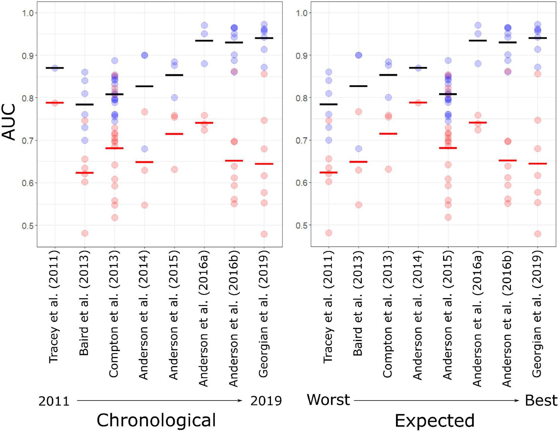
Figure 2. AUC values generated using internal cross-validation (blue) and independent test data (red) for individual habitat suitability models in eight published studies (S1–S8, see Table 1 for details) in order of time of publication from 2011 to 2019 (Left), and a priori ranking of expected model performance based on the criteria of Araujo et al. (2019) (Right). Cross bars show mean values for each study.

FIGURE 3

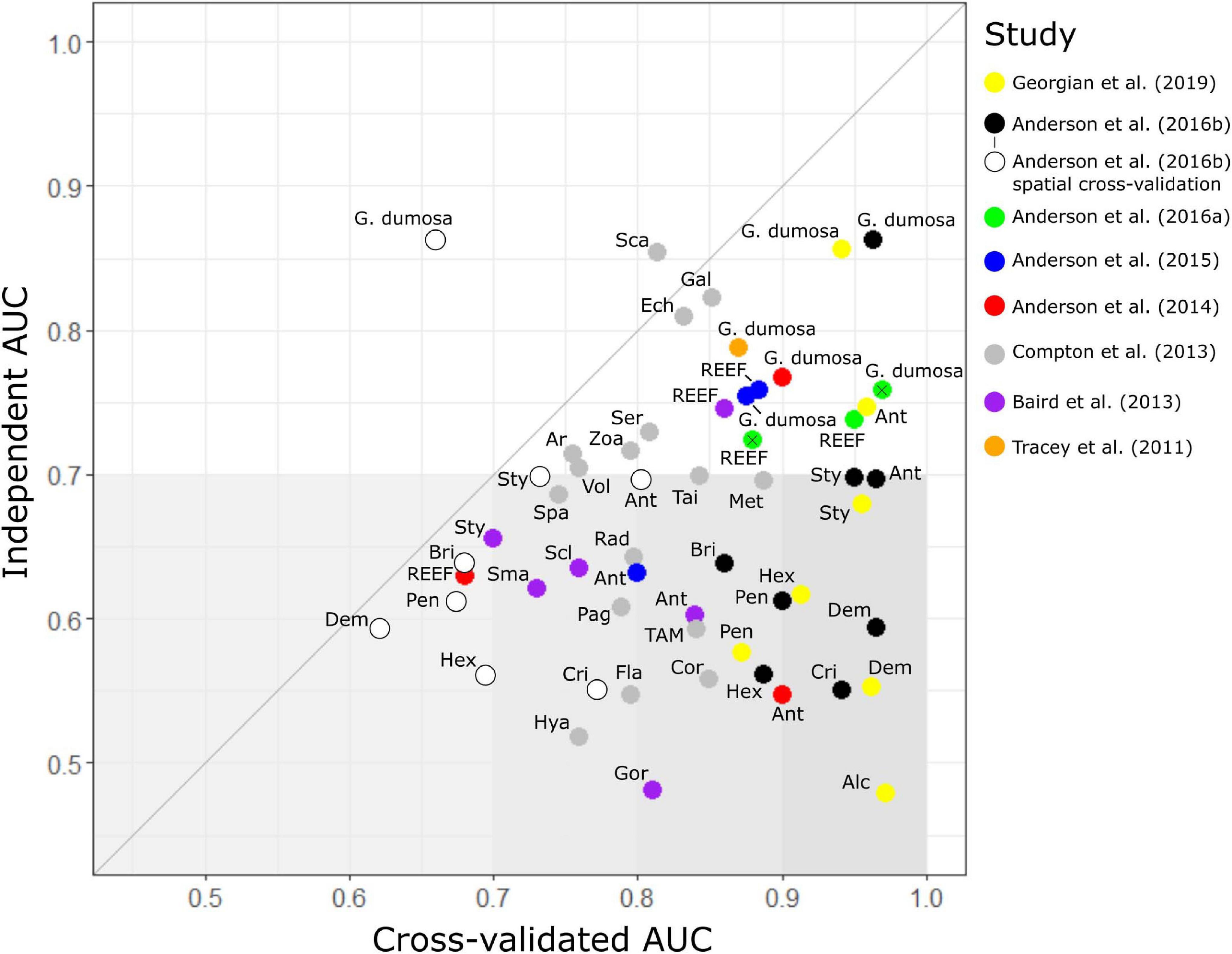
Figure 3. Model assessment. Comparison of benthic invertebrate species-distribution model performance (as area under the receiver operator curve, AUC) when assessed against sample data withheld from the original dataset used to build the models (internal AUC) and an independent dataset of faunal distributions derived from photographic surveys (independent AUC). The 48 models are from eight published studies (see text for details) and cover 29 taxa: Alcyonacea (Alc); Anthomastus robustus (Ar); Antipatharia (Ant); Brisingidae (Bri); coral reef-forming taxa (REEF); Corallimorpharia (Cor); Crinoidea (Cri); Demospongiae (Dem); Gracilechinus multidentatus (Ech); Echinothuroida (TAM); Flabellum spp. (Fla); Galatheidae (Gal); Goniocorella dumosa; Hexactinellida (Hex); Gorgonacea (Gor); Hexactinellida (Hex); Hyalinoecia tubicola (Hya); Metanephrops challengeri (Met); Paguridae (Pag); Pennatulacea (Pen); Radicipes spp. (Rad); Scaphopoda (Sca); Scleractinia (Scl); Serolidae (Ser); small solitary corals (Sma); Spatangidae (Spa); Stylasteridae (Sty); Taiaroa tauhou (Tai); Volutidae (Vol), and Zoanthidae (Zoa). Anderson et al. (2016a) modeled REEF and G. dumosa with BRT and MaxEnt separately; MaxEnt results are indicated with a cross. Anderson et al. (2016b) calculated AUC in two ways: random selection of sites (black plots) and in longitudinal bands (white plots). Gray line shows a 1:1 relationship between internal and independent AUC scores, and gray shading indicates independent AUC scores less than 0.7, a value above which models are considered to be potentially useful for prediction, with darker shading to highlight the largest discrepancies between internal and independent AUC values.

The two models that scored more highly against the independent test data (AUC_ind > AUC_kcv) were those for the molluscan class Scaphopoda in Compton et al. (2013) and the stony coral G. dumosa in Anderson et al. (2016b). For the latter model, however, this was only the case when AUC_kcv was calculated using spatial banding in cross validation. Of the remaining 29 models, 22 had AUC_ind values of less than 0.65, despite all but one of these (REEF in Anderson et al., 2014) scoring higher than 0.7 by internal cross-validation. The exceptions here, again, were the models in Anderson et al. (2016b) in which spatial banding was used to generate AUC_kcv. For these models, AUC_kcv values were less than 0.7 and closer to, but still higher than, their AUC_ind values.

The highest published cross-validation values (AUC_kcv > 0.9) were all from the three most recent studies (Anderson et al., 2016a,b; Georgian et al., 2019) but the corresponding AUC_ind values for these studies ranged widely, including both the highest (0.86 for G. dumosa) and lowest (0.52 for Alcyonacea) scores. Only two of the seven models from Georgian et al. (2019) and three of the eight from Anderson et al. (2016b) scored AUC_ind values of 0.7 or higher (G. dumosa and Antipatharia in both studies, and Stylasteridae in Anderson et al., 2016b) but both the MaxEnt and BRT models for REEF from Anderson et al. (2016a) scored above 0.7. There was a trend for AUC_ind to increase at finer taxonomic resolution but this was not matched in AUC_kvc values (Supplementary Figure 1), with strongly divergent values at Class level becoming more similar to AUC_ind values at finer resolutions. The increasing trend in AUC_ind at finer taxonomic resolution was associated with increases in the true positive rate (sensitivity), rather than the true negative rate, which showed no trend across taxonomic levels.

True skill statistic was strongly correlated with AUC_ind (R² = 0.92). Only six models yielded TSS values greater than 0.5, three of these scoring 0.6 or higher (Table 3), and the best-performing models were the same as identified by the AUC analysis.

TABLE 3

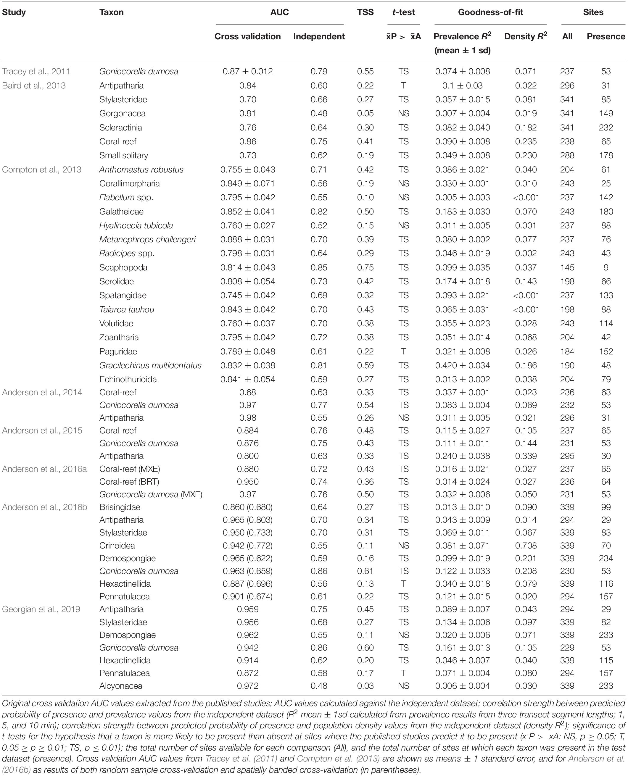
Table 3. Model assessment results.

t-Tests

For 35 of the 47 published models (74.5%), mean predicted probability of suitable habitat was significantly higher (TS, p < 0.01) at sites where the modeled taxon was present, rather than absent, in the independent data, with another four models included at the lower significance level (T, p < 0.05) (Table 3). For the remaining 8 models (“NS” results), the mean predicted probability of suitable habitat was never higher for absence sites than for presence sites. Twelve of the TS models were from Compton et al. (2013) but there were significant (TS) results for models in all studies and the proportions of significant results in each of the studies that modeled more than 3 taxa were broadly comparable: Baird et al. (2013), 66.6%; Compton et al. (2013), 75.0%; Anderson et al. (2016b), 75.0%, and Georgian et al. (2019), 57.1%. The models that scored as TS spanned a range of taxonomic levels, including species (Goniocorella dumosa, Anthomastus robustus, Metanephrops challengeri, Taiaroa tauhou, and Gracilechinus multidentatus), Genus (Radicipes), Family (Galatheidae, Serolidae, Spatangidae, Volutidae, and Stylasteridae), Order (Scleractinia, Alcyonacea, Antipatharia, Brisingida, Zoantharia, and Pennatulacea), and Class (Demospongiae and Hexactinellida). However, except for G. dumosa, which was modeled in six of the eight studies, all of the species-level models and the models for Radicipes, Galatheidae, Serolidae, Spatangoida, Volutidae, and Brisingida were from the Compton et al. (2013) study, which used occurrence data primarily from photographic sampling.

Correlations With Taxon Prevalence and Density

Correlations between predicted probability of suitable habitat in the published models and values of both prevalence and population density in the independent dataset were weak (R²_prev < 0.25 for 46 of the 47 models, and R²_dens < 0.25 for 45 of the 47 models). The three cases where correlation strength exceeded 0.25 were models for the echinoid G. multidentatus (R²_prev = 0.42 in Compton et al., 2013), the black coral Order Antipatharia (R²_dens = 0.34 in Anderson et al., 2014), and the Order Crinoidea (R²_dens = 0.71 in Anderson et al., 2016b). Across all other models, the mean correlation strength against both prevalence and density values in the independent dataset was less than 0.1 (mean ± sd: R²_prev = 0.071 ± 0.052, R²_dens = 0.078 ± 0.121). The high R²_dens value for Crinoidea in Anderson et al. (2016b) was driven by very high densities of crinoids on the Graveyard seamounts, which were within the area of high predicted probability of suitable habitat in this model.

Realized Rank Performance

When the models were ranked by their average rank results across all evaluation metrics, there was a broad spread of performance within and among studies. The 10 highest-ranked models were spread across 6 studies from 2013 to 2019, the 10 lowest-ranked models included two from the most recent study, and mean ranking by study showed no indication of a general trend of improvement over time (Figure 4). Of the four taxa that were modeled in more than two studies (G. dumosa, Coral reef, Stylasteridae, and Antipatharia), G. dumosa was the most consistently highly ranked, with five of its six models in the top fifteen. G. dumosa models also showed some indication of improving performance over time, as did Stylasteridae, with models from the two most recent studies ranking higher than those from earlier studies (Figure 4).

FIGURE 4

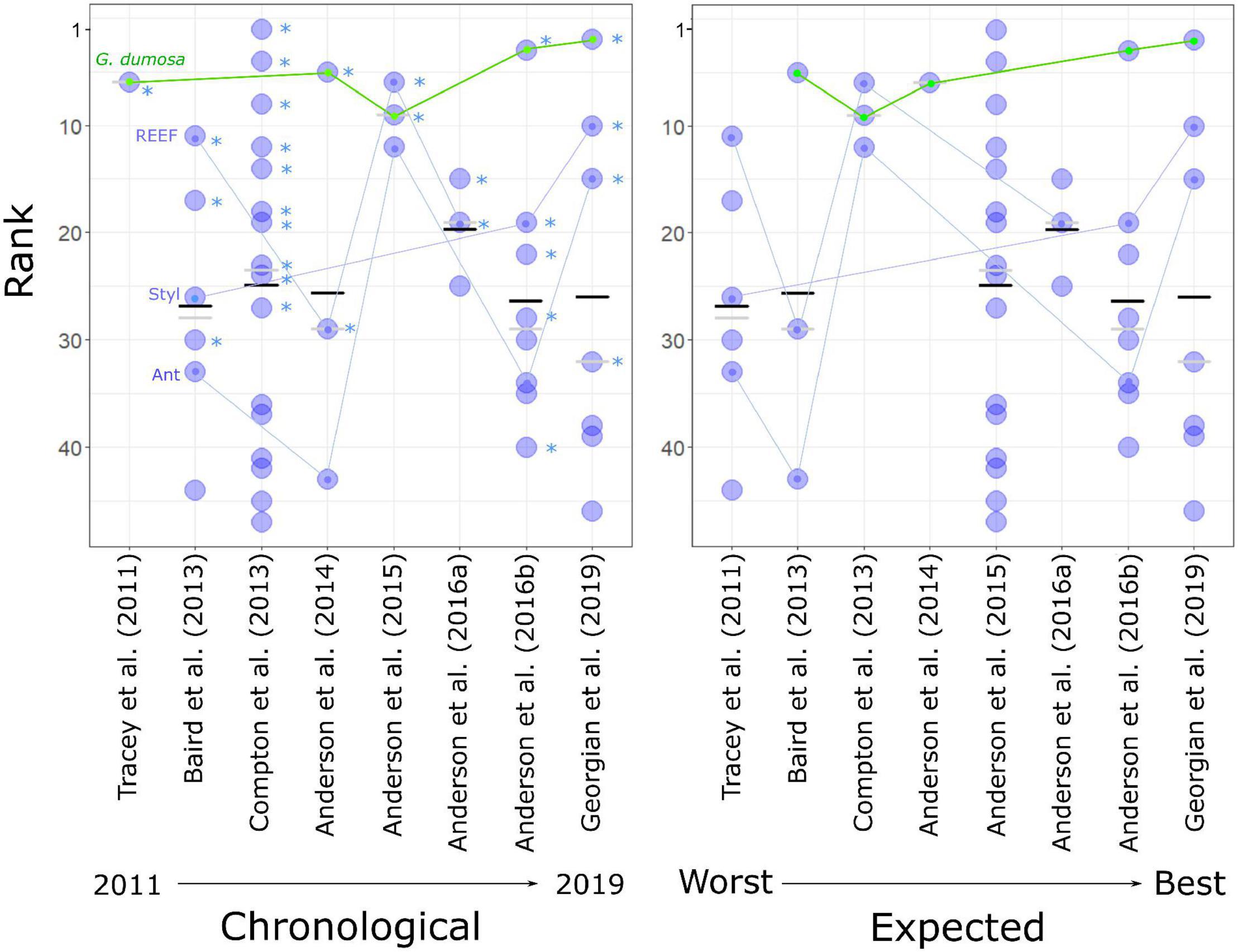
Figure 4. Rank performance of 47 predictive models, showing average rank across four evaluation measures (TSS, t-test, R²_prev, and R²_dens) for each model (blue dots), and the mean (black bars) and median (gray bars) ranking for each study (S1–S8). (Left) studies in chronological order, asterisks indicate models for which the average predicted probability of suitable habitat for the target taxon was significantly higher (t-test, p < 0.01, “TS”) at sites where that taxon was present in the independent dataset than at those where it was absent. Four taxa that were modeled in more than two studies are linked by lines (see Figure 3 for full names). (Right) with studies ordered by their expected rankings as assessed by reference to the standards of Araujo et al. (2019).

The spread of high- and low-ranked models across studies was such that no overall ranking of the studies could be assigned with confidence (Figure 4). There was, however, neither evidence for substantially improved performance from earlier to later models nor support for the rankings assigned by reference to Araujo et al. (2019) prior to the evaluation exercise.

Discussion

In this study, we have used independent data from seabed photographic surveys to explore the general utility of habitat suitability models that we have developed over more than 10 years with the aim of predicting distributions of seafloor taxa in the southwest Pacific, centered on New Zealand. The key results of our assessment are that (1) measured model performance was lower when assessed against independent data than by k-fold cross-validation for all but two of 47 models; (2) a trend of increasing model performance with time, which is seen in published cross-validation (AUC_kcv) values and is anticipated when the methods used in these studies are judged against objective criteria, is not supported when the models are tested against independent data; (3) for approximately 72% of the models, predicted probability of suitable habitat in the models was significantly higher at sites where a taxon was present in the independent data than where it was absent; and (4) correlation strengths between predicted probability of presence and observed taxon prevalence and density were weak.

While the third result here is the only statistic that offers support for the expectation that such models might be reliable for predicting distributions, and then only at the level of prediction of presence, the results overall should also be viewed in the context of how realistic our expectations of such models are. A key aspect here is that Chatham Rise is in a highly dynamic oceanographic environment and encompasses a wide range of seafloor topographies within a relatively confined spatial extent (Nodder et al., 2012). Thus, although the Rise is one of the areas within New Zealand’s EEZ that we are most interested in predicting to, because of its importance to commercial fisheries (Fisheries New Zealand, 2020) and potential mineral interests (Von Rad and Kudrass, 1987), it is also likely to be one of the most challenging. Perhaps more importantly for future work in this field, the evaluation exercise affords the chance to review our expectations and to explore which aspects of the models, in terms of input data, spatial scope, and modeling methods, contribute most to the observed differences in performance against the independent data. We use this evaluation to suggest future directions for model building that should produce models that can be used with greater confidence for environmental management.

Cross-Validation and Non-independence of Data

Several studies have demonstrated that model performance metrics generated by the common practice of cross-validation using withheld subsets of the input sample data will yield inflated values (e.g., Bahn and Mcgill, 2013; Valavi et al., 2019) because the withheld data are not independent of those used to train the model, particularly with respect to spatial autocorrelation (Bahn and Mcgill, 2007; Ploton et al., 2020). It is interesting here, however, that AUC values for most models in the two studies that made explicit allowance for spatial structure in the sample data, whether by withholding data in longitudinal bands (Anderson et al., 2016b) or by including spatial autocorrelation as a predictor variable (Georgian et al., 2019), were still inflated by comparison with those calculated against the independent data. This finding suggests that neither of these methods entirely overcame the issue of non-independence of data and, thus, that issues associated with using cross validation as a primary method for model performance are not easily overcome. Awareness of the need to account for spatial structuring of data in habitat suitability models is increasing, and availability of new, more flexible, tools now allows for more nuanced approaches that are likely to improve estimation of predictive performance by cross-validation (Valavi et al., 2019).

Regardless of the absolute values obtained from AUC analyses, our finding that the trend of increasing model performance with time was not supported against the independent data is concerning for two reasons: firstly, because our results show that we do not appear to be getting substantially better at describing distributions and, more importantly, because if apparent increases in performance encourage overconfidence in predictions from more recent models, it could lead to poor environmental management decisions (Regan et al., 2005). If our modeling methods have, indeed, improved over time, however, this result is also revealing because it suggests that the main impediments to accurate prediction are associated primarily with the quality and quantity of the input sample and environmental data, rather than with the details of specific modeling methods. This suggestion is further supported by the broad spread of AUC_ind values within individual studies in our results, with both the highest and lowest values being for models generated in the most recent, most technically sophisticated study (Georgian et al., 2019), and comparably high and low values recorded from earlier studies.

In our initial assessment of the studies against the standards of Araujo et al. (2019), the principal areas we characterized as being either “deficient” or “bronze” in all studies were understanding variability and uncertainty in the predictor variables (Issue 2C), and dealing with modeling and parameter uncertainty (Issue 3D). It was also clear, however, that the reliability and precision of taxon identification (Issue 1B) were likely to influence model performance. Thus, although our ranking was at the level of study, any assessment of how well taxon identification had been addressed in studies that covered multiple taxa would ideally be at the level of individual models, rather than the whole study, because of wide differences in how taxa were grouped.

Uncertainty in Predictor Variables

Uncertainty associated with the predictor variables used in the models was the area of greatest concern in the initial model assessments, with questions around the lack of some key ecologically relevant variables, limitations of spatial resolution, and the reliability of predictor layers that are themselves outputs from spatial modeling or interpolation processes (Davies and Guinotte, 2011). These issues affect all broad-scale habitat suitability modeling initiatives in the deep sea and present unique challenges by comparison with terrestrial studies, which often have the benefit of greater accessibility for direct sampling and full-coverage, high-resolution, remote sensing by satellite (e.g., Pearce and Ferrier, 2001; Parmentier et al., 2011; Ploton et al., 2020).

The lack of key variables is a fundamental issue affecting prediction of the distributions of seabed fauna. Substrate type in particular is a determinant of realized distributions for most benthic taxa, but our knowledge about the occurrence of substrate types in the deep sea at anything beyond highly local scales is of qualitatively the same type as our knowledge of the fauna we are interested in predicting: patchy, spatially auto-correlated, point sample records collated from multiple sources. Despite recent initiatives to generate continuous substrate-type layers by interpolation among point samples in our region (e.g., Bostock et al., 2019), these characteristics currently render such layers unreliable for use in predictive models (Georgian et al., 2019). In a study area that has been subject to modification by bottom-contact trawl fisheries for decades (Bowden and Leduc, 2017; Baird and Mules, 2019; Clark et al., 2019), it is also of note that none of the models assessed here included fishing effort as a predictor variable. While fishing might be expected to vary in location and intensity over finer spatial and temporal scales than most environmental variables, and thus have inconsistent influence on realized faunal distributions, it is also likely that any influence it does exert is likely to be strong in some habitats. The present distributions of cold-water scleractinian corals on seamounts and other topographic features that have been targeted by trawling, for instance, have been modified from their natural state (Williams et al., 2010, 2020; Clark et al., 2019) and thus are unlikely to be predicted accurately by models that do not incorporate fishing effort as a predictor of presence.

While some environmental variables commonly used in deep-sea habitat suitability models are derived directly from full-coverage satellite remote sensing (e.g., sea surface temperature, chlorophyll a concentration), or acoustic remote sensing [e.g., multibeam echosounder (MBES) for smaller-scale studies], many others are derived indirectly from discrete sample data (e.g., single-beam acoustic soundings, CTD casts, and Argo floats), either by spatial interpolation (regional bathymetry and, thus, all topographic variables derived from it, including seabed slope, curvature, rugosity, and position index) or via modeling of physical (e.g., seabed currents and temperature), chemical (e.g., salinity and aragonite saturation), or biogeochemical (organic carbon flux to the seabed) processes. Furthermore, in modeling studies of seafloor fauna, values for individual grid cells are necessarily extracted by reference to the bathymetry layer (Davies and Guinotte, 2011), which as noted above, at spatial scales greater than local MBES surveys, carries its own unquantified uncertainty. Thus, all of the environmental data layers relied upon as predictor variables in habitat suitability modeling initiatives in the deep sea introduce some degree of additional, usually unquantified, uncertainty into the final predictions.

Formal analysis of the influence of inaccuracies in environmental variable layers used as predictors in SDM models is beyond the scope of this study, but some of the issues are illustrated by one of the studies assessed here (Anderson et al., 2016a), in which we ran a purpose-designed photographic survey of seamount features in the Louisville Seamount Chain to assess the reliability of predictions from habitat suitability models we had generated for the entire SPRFMO Convention Area. We found that our models were not successful at predicting occurrence of scleractinian corals at the scale of the survey, despite high AUC values for the models from internal cross-validation. We attributed this failure primarily to inaccuracies in the bathymetry layer at the spatial resolution of the model and to the lack of a predictor variable describing substratum type. Inaccuracies in the bathymetry later were compounded in all other predictor variables derived from it, including seafloor slope and rugosity, while the absence of hard substrata across large proportions of the seamount summits confounded predictions of high habitat suitability because hard substrata are a fundamental habitat requirement for the corals we were predicting. While these factors were probably exacerbated by the steep topography and isolated oceanic context of the Louisville seamounts, results in the present assessment indicate that the Anderson et al. (2016a) models fare no better against survey data from Chatham Rise, where bathymetric data are much more reliable and where much of their input faunal occurrence data were collected.

Modeling and Parameter Uncertainty

Acknowledging uncertainty in the predictor variables leads to the issue of how to deal with modeling and parameter uncertainty (Issue 3D in Araujo et al., 2019) because in deep-sea models the predictor variables are likely to be the largest source of uncertainty, for the reasons discussed above. Modeling uncertainty was considered explicitly in only three of the eight studies considered here (Anderson et al., 2016a,b; Georgian et al., 2019), but in each case it was quantified only in terms of the influence either of using different subsets of the response variable (taxon) data, or of using different modeling methods, or both, with no quantification of the uncertainty associated with the environmental predictor layers used. Thus, for all studies considered here, the largest potential source of uncertainty in the final model predictions remained unquantified. Our current inability to account for the uncertainty associated with the environmental layers used as predictors in habitat suitability models for the deep sea is a major impediment to increasing confidence in the predictions of such models (e.g., Kenchington et al., 2019).

Another rarely acknowledged source of uncertainty in habitat suitability models for the deep sea is that taxon occurrence data are, in most cases, compiled from sources that span periods of years, decades, or even centuries. This is a practical way to compensate for the general paucity of data available from deep-sea environments, which results from the logistical difficulty and cost of sampling at depth (Clark et al., 2016). All but one of the studies assessed here used data compiled over extended periods (e.g., Tracey et al., 2011 used coral occurrence data from 1955 to 2009), the exception being the study of Compton et al. (2013), in which models were trained on data from surveys conducted within 2 years of each other and only 2 years before the modeling work was undertaken. Two important assumptions are implicit when occurrence data are accumulated over extended periods: first, that patterns of occurrence will not have changed materially during the entire period from the date of the first occurrence record to production of the model predictions, and second, that the environmental characteristics used as predictors (the summaries for which are likely to represent somewhat different periods to those over which taxon records are accumulated) will not have changed materially either. For long-lived sessile taxa, such as cold-water corals, the first assumption might be reasonable in many cases. However, with increasing evidence of the effects of bottom-contact fishing and other anthropogenic and natural disturbances on realized occurrences (e.g., Clark et al., 2000, 2019, Mountjoy et al., 2018), and parallel increases in our understanding of the rates of large-scale environmental change resulting from global warming (Smith et al., 2009; Hoegh-Guldberg and Bruno, 2010; Doney et al., 2012), such assumptions become increasingly tenuous.

Taxonomic Resolution

Our study showed that there was a tendency for models of finer taxonomic levels to perform better against the independent data than those at a coarser level (Supplementary Figure 2). Aggregating records to coarser taxonomic groupings is common in studies of deep-sea benthic invertebrate distributions, where records are often collated from multiple sources at differing levels of identification and where available records at finer levels (species or genus) can be too sparse to inform habitat suitability models. This issue is not covered explicitly by Araujo et al. (2019) but is likely to have a strong influence on the predictive success of models because coarser taxonomic groupings encompass taxa with different adaptations and environmental tolerances, which, when combined in a single model, may lead to predicted distributions that are too general to be useful. Effects of aggregating to coarser taxonomic levels are evident in our results, with the broadest groups modeled, including Alcyonacea (soft corals), Gorgonacea (gorgonian corals), Demospongiae (sponges), and Hexactinellida (glass sponges), generating among the lowest AUC_ind values and overall rank performances. An important observation here is that the models for these taxonomic groups are also potentially the most misleading because, in contrast to their performance against the independent data, they scored highly when assessed by cross validation—all models for the VME indicator taxa Demospongiae and Hexactinellida in the most recent studies (Anderson et al., 2016b; Georgian et al., 2019), for instance, yielding AUC_kcv values greater than 0.87, indicating “reliable” or “excellent” performance. While these contrasting patterns of model performance in relation to taxonomic resolution are intriguing and suggest an important direction for further investigation, the results here should be viewed with some caution because of confounding factors in the data available to this study. For instance: the numbers of taxa within taxonomic levels are unequal; taxonomic levels are not represented evenly across studies, thus introducing potential methodological bias; some reported taxonomic levels are potentially inaccurate (as we determined for the group Scaphopoda), and most of the species-level models are for a single taxon, G. dumosa, which was modeled using essentially the same response variable data in all models.

These issues notwithstanding, comparison between two taxa with the highest- and lowest-ranked models in our analysis, the scleractinian coral G. dumosa and sponges (Porifera, modeled as two Classes: Demospongiae and Hexactinellida, in Anderson et al., 2016b; Georgian et al., 2019), illustrates the probable influence of taxonomic resolution on model performance. G. dumosa is consistently identified to species level because it has a protected status in New Zealand and is of high conservation interest due to its provision of complex biogenic habitat. However, G. dumosa occurrence records are also clustered within relatively narrow environmental and spatial bounds, with the highest density of records used to inform all of the models assessed here coming from Chatham Rise itself (e.g., Tracey et al., 2011; Anderson et al., 2016b). Sponges, by contrast, are highly diverse and difficult to identify to species and thus are typically modeled at the coarse taxonomic level of Class (Demospongiae and Hexactinellida). Grouped at this level, occurrence records for sponges are spread much more widely across environmental gradients than would be the case for individual species. Given these differences in their input data, the task of modeling distributions is clearly simpler for G. dumosa than for the sponge classes and it is not surprising that their respective models ranked as they did, despite being modeled using the same methods and the same predictor variables.

The study of Compton et al. (2013) is interesting here because, unlike all the other studies, its models were based on data from two surveys designed specifically to sample seafloor invertebrate communities using high-resolution photographic transects and epibenthic sled samples. Only one of the surveys covered Chatham Rise (TAN0705), and the resulting density of sample points for both presences and absences was, therefore, lower than for the other studies. However, because photographic survey methods yield close to 100% detection of epibenthic invertebrates, a high proportion of taxa were identified reliably and consistently to species or genus level and it was possible to use true absence data, rather than random background absences, target-group absences, or pseudo-absences. We expected the fine taxonomic resolution and availability of true absence data to yield improvements in model predictions compared to other studies, but while some models from the study are among the highest ranked in our assessment (e.g., Scaphopoda, Galatheidae, and Gracilechinus multidentatus), others are among the lowest (e.g., Hyalinoecia tubicola, Flabellum spp.) and the overall range of results is comparable with other studies. Given that the sampling methods and taxonomic resolution scored highly against the evaluation criteria, the two key aspects remaining that might explain the overall performance are, again, uncertainty in the environmental predictor variables and the relatively low density of sampling for the response variables.

Measuring Prediction Success

The metrics used to evaluate models here were chosen to assess how useful the model predictions are likely to be in practical applications, the primary intended use for such predictions being to inform management and conservation decisions across a range of spatial scales (km to 100s km) within the model domain (Anderson et al., 2016a; Araujo et al., 2019; Winship et al., 2020). Thus, in addition to the well-established AUC and TSS metrics, we used the three simpler measures that were intended to reflect naïve questions about a taxon’s distribution at differing levels of predictive skill: is it likely to be present at a given site? (t-tests); what is its prevalence likely to be at that site? (R²_prev), and what is its abundance likely to be at that site? (R²_dens). While these are simplistic measures of model performance, not least because any relationship between predicted probabilities and measured occurrences is unlikely to be linear and realized occurrences and densities are likely to be influenced by historical events, ecological interactions, and stochastic processes (Dayton and Hessler, 1972; Connell and Slatyer, 1977; Connolly and Roughgarden, 1999), they provide intuitively interpretable measures of how well the model predictions match the independent observations and, thus, our expectations of a model’s predictive ability.

The models evaluated here can only predict the probability of suitable habitat being present at a given site, which in itself is of limited use for most applications (Bahn and Mcgill, 2013), but continuous maps based on these probabilities inevitably invite the interpretation that higher predicted habitat suitability should correspond with higher population densities of the target taxon (Lobo et al., 2008). This interpretation is not justifiable from a theoretical perspective, but it is, arguably, the way in which outputs from habitat suitability models are often viewed. Indeed, it is arguable that if such an interpretation is not at least partially justified, we should question what purpose such predictions serve, if not to indicate where a taxon is most likely to be found. In this context, an important result here is that most correlations between predicted probability of suitable habitat being present and observed densities of taxa on the seabed were weak. This is a practical demonstration that inferring the likelihood of taxon occurrence or population density from predictions of suitable habitat being present is, indeed, unlikely to be justified.

Prediction of presence or absence is less demanding than prediction of relative or absolute density (Bahn and Mcgill, 2013), so it is not surprising that models generally performed better against the presence–absence tests (AUC, TSS, and t-tests) than against the quantitative ones (R²_prev, and R²_dens), the most encouraging results being from tests of the simple expectation that modeled probabilities of suitable habitat would be significantly higher at sites where a given taxon was present in the independent data than at those where it was absent. At this level of predictive skill, 72% of models met the expectation at the more conservative level (TS, p = 0.01), offering some support for the utility of existing models in practical applications that require only prediction of likelihood of presence. However, that there was no pattern of general improvement against this test with increasing sophistication of modeling methods suggests that performance is limited more by the quality and quantity of input data than by analytical methods, and for the more interesting and potentially useful task of predicting taxon densities, there is no support.

Despite all but a few of the models performing less well than was anticipated from their original cross-validation scores, some emerge as being potentially useful for reliable prediction of taxon occurrence at unsampled sites. Thus, models that performed well against the independent data and predicted the occurrence of suitable habitat for taxa that have high management or conservation status might be used with some confidence in spatial management (Moilanen et al., 2006). In our case, these criteria would limit the set of potentially useful predictions to those for the scleractinian coral G. dumosa (Figure 5), and the combined grouping of reef-forming scleractinian corals (REEF, Figure 6). For the few taxa that have been modeled in more than one study, notably G. dumosa, models from the most recent studies (Anderson et al., 2016b; Georgian et al., 2019) performed better than earlier ones. However, the difference in performance between the earliest (Tracey et al., 2011) and latest (Georgian et al., 2019) models for G. dumosa was relatively minor, and the most recent studies also included some of the lowest-ranked models in our comparison. This finding suggests, again, that any benefits gained from refinement of modeling methods may be small by comparison with other aspects of the model-development process, including the quantity and spatial distribution of occurrence data, the taxonomic level and consistency of identifications, and the availability of reliable and appropriate environmental layers at ecologically relevant spatial scales.

FIGURE 5

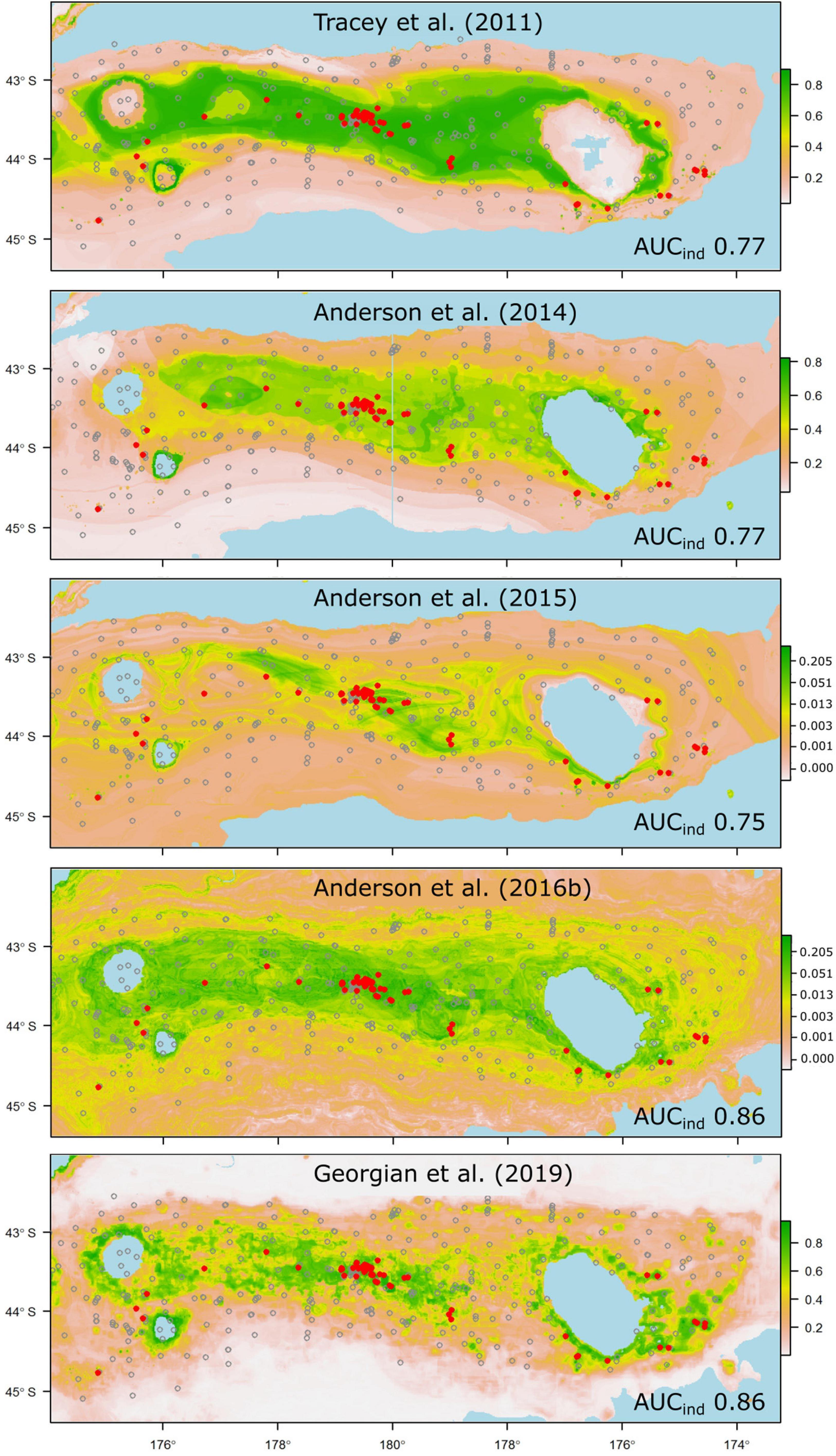
Figure 5. Probability of suitable habitat for the branching scleractinian coral Goniocorella dumosa on Chatham Rise, as predicted by habitat-suitability models in five published studies. Probability values are scaled at right, and prediction maps are overlaid with presence (red dots) and absence (gray circles) locations from the independent photographic observation dataset. AUC values from testing against the independent dataset are shown for each model (AUC_ind).

FIGURE 6

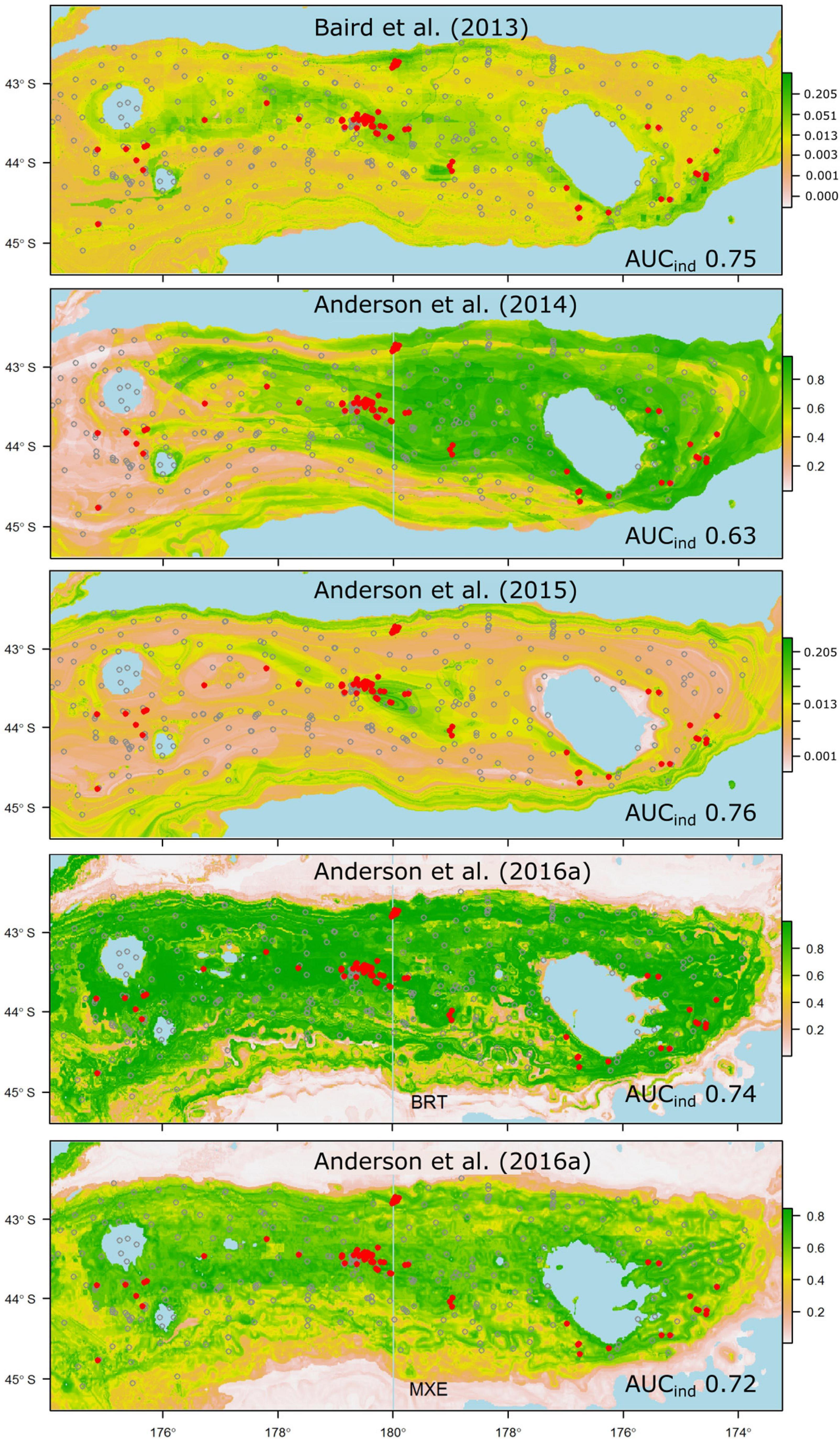
Figure 6. Probability of suitable habitat for all thicket- or reef-building Scleractinian corals (Solenosmilia variabilis, Madrepora oculata, Enallopsammia rostrata, and Goniocorella dumosa) on Chatham Rise, as predicted by habitat-suitability models in four published studies. Anderson et al. (2016a) produced two models for reef-building corals, one using BRT, the other MaxEnt (MXE). Probability values are scaled at right, and prediction maps are overlaid with presence (red dots) and absence (gray circles) locations from the independent photographic observation dataset.

Conclusion

For habitat suitability models to be useful in deep-sea environmental management applications, we need to have confidence that their predictions are reliable at appropriate spatial scales and taxonomic resolutions. A first step toward this should be routine use of cross-validation methods that account for spatial structuring in the input data. Reliability can only be confirmed, however, by assessing model predictions against independent data using methods that sample the target taxa effectively, our results demonstrating that such assessments can yield a very different picture of prediction success than is gained from cross-validation methods. While it is concerning that most of our current model predictions are apparently of limited use for their intended applications in management, the process of objective assessment helps to identify which aspects of the modeling process are most in need of improvement. Limitations in the quality and quantity of input data, for both response and predictor variables, appear to be the primary factors affecting prediction success, rather than details of the modeling methods used. If this is the case, increased confidence in the outputs from future models will probably be achieved only by greater investment in data collection and in quantifying the uncertainty associated with these data, for both response and predictor variables. Generating more reliable environmental data, particularly bathymetry, at spatial resolutions relevant to the habitat preferences of target taxa will be a critical component of this, with initiatives such as the Irish National Seabed Survey (O’toole et al., 2020) and Seabed 2030 Project (Mayer et al., 2018), exemplifying the scale of commitment required. In parallel with this, it seems likely that dedicated surveys of taxon distributions will always be necessary, both to validate existing models and to enhance data inputs for their successors.

Despite the generally disappointing performance of our models in this assessment, they can serve as useful heuristics if viewed as hypotheses to be tested. Approached in this way, we suggest that a practical long-term strategy to reduce uncertainty in model predictions can be structured around iterations of a 4-step cycle in which (1) initial habitat suitability modeling based on all available taxon occurrence data generates predictions, (2) these predictions are used to structure field validation surveys, (3) survey data are used for objective evaluation of prediction success, and (4) the survey data are then integrated with existing data and used to develop revised models. Predicting to overlapping seabed areas at each iteration of the cycle would progressively expand the environmental and spatial scope of the models while staying within the bounds of ecological credibility. The present study represents stage 3 of the first iteration of this cycle in New Zealand but as we note above, our results show that major sources of uncertainty in our models, including the quality, spatial resolution, and ecological relevance of the environmental predictor variables, have yet to be addressed adequately.

Data Availability Statement

Data used in this study are publicly available via links in the published studies and reports available here: https://marinedata.niwa.co.nz/quantifying-benthic-biodiversity/.

Author Contributions

DB, AR, and MC conceived the study. DB compiled independent test data. OA ran model assessments. OA and DB analyzed results. DB led manuscript writing, with all authors contributing throughout the process.

Funding

This study was commissioned and funded by the New Zealand Ministry for Primary Industries (MPI), now known as Fisheries New Zealand (FNZ), under project ZBD201611 Quantifying Benthic Biodiversity, with additional support through NIWA Strategic Science Investment Fund project COES1801 Marine Food Web Dynamics. The following past and present agencies contributed to funding of the various models assessed in this study: MPI; the Foundation for Research Science and Technology; the Department of Conservation; and the Ministry of Business Innovation and Employment.

Conflict of Interest

The authors declare that the research was conducted in the absence of any commercial or financial relationships that could be construed as a potential conflict of interest.

Acknowledgments

We thank Mary Livingston for project governance at FNZ, Caroline Chin, Niki Davey, Alan Hart, Rob Stewart, and Megan Carter at NIWA for their meticulous image analysis work, and the officers and crew of RV Tangaroa on the camera survey voyages that made this analysis possible. Lastly, we acknowledge the initial thought- and action-provoking discussion with Alistair Dunn, Martin Cryer, Richard Ford, and Mary Livingston of MPI, who challenged us to demonstrate that the habitat suitability models we had developed for benthic fauna could be considered useful for fisheries management.

Supplementary Material

The Supplementary Material for this article can be found online at: https://www.frontiersin.org/articles/10.3389/fmars.2021.632389/full#supplementary-material

Supplementary Figure 1 | Illustration of prevalence calculation, showing the seabed track of a video transect (Voyage TAN0705, station 170) divided into 10-min segments (alternating blue–red), with individual observations of the taxon Paguridae (hermit crabs) indicated by black circles. Prevalence is calculated as the proportion of the total number of segments in which the taxon was observed, in this case 8/12 = 0.66. Also shown are the density of Paguridae as individuals 1,000 m^–2, and the probability of suitable habitat as predicted by the BRT model of Compton et al. (2013).

Supplementary Figure 2 | Variation in AUC and Sensitivity (true positive rate) with taxonomic resolution. (Left) AUC_kvc (by cross validation, blue) and AUC_ind (against independent data, red) values as described in Figure 3, plotted by taxonomic level. (Right) Sensitivity (true positive rate) for all models when assessed against the independent data. Horizontal bars show mean values in each taxonomic level.

Supplementary Table 1 | Author’s ranking of eight published SDM studies by reference to assessment criteria and issues proposed by Araujo et al. (2019). DB, David Bowden; OA, Owen Anderson; AR, Ashley Rowden; FS, Fabrice Stephenson. Rankings from best to worst are: gold (G); silver (S); bronze (B), and deficient (D).

References

Allouche, O., Tsoar, A., and Kadmon, R. (2006). Assessing the accuracy of species distribution models: prevalence, kappa and the true skill statistic (TSS). J. Appl. Ecol. 43, 1223–1232. doi: 10.1111/j.1365-2664.2006.01214.x

CrossRef Full Text | Google Scholar

Anderson, O. F., Guinotte, J. M., Rowden, A. A., Clark, M. R., Mormede, S., Davies, A. J., et al. (2016a). Field validation of habitat suitability models for vulnerable marine ecosystems in the south pacific ocean: implications for the use of broad-scale models in fisheries management. Ocean Coastal Manag. 120, 110–126. doi: 10.1016/j.ocecoaman.2015.11.025

CrossRef Full Text | Google Scholar

Anderson, O. F., Guinotte, J. M., Rowden, A. A., Tracey, D. M., Mackay, K. A., and Clark, M. R. (2016b). Habitat suitability models for predicting the occurrence of vulnerable marine ecosystems in the seas around new zealand. Deep-Sea Res. Part I-Oceanogr. Res. Papers 115, 265–292. doi: 10.1016/j.dsr.2016.07.006

CrossRef Full Text | Google Scholar

Anderson, O. F., Mikaloff Fletcher, S. E., and Bostock, H. C. (2015). Development of Models for Predicting Future Distributions of Protected Coral Species in the New Zealand region. NIWA Client Report to Department of Conservation No. WLG2015-65, 28.

Google Scholar

Anderson, O. F., Tracey, D. M., Bostock, H. C., Williams, M., and Clark, M. R. (2014). Refined Habitat Suitability Modelling for Protected Coral Species in the New Zealand EEZ. No. National Institute of Water and Atmsopheric Research, Report No. WLG2014-69, 46.

Google Scholar

Araujo, M. B., Anderson, R. P., Barbosa, A. M., Beale, C. M., Dormann, C. F., Early, R., et al. (2019). Standards for distribution models in biodiversity assessments. Sci. Adv. 5:eaat4858. doi: 10.1126/sciadv.aat4858

PubMed Abstract | CrossRef Full Text | Google Scholar

Araujo, M. B., and Guisan, A. (2006). Five (or so) challenges for species distribution modelling. J. Biogeogr. 33, 1677–1688. doi: 10.1111/j.1365-2699.2006.01584.x

CrossRef Full Text | Google Scholar

Bahn, V., and Mcgill, B. J. (2007). Can niche-based distribution models outperform spatial interpolation? Global Ecol. Biogeogr. 16, 733–742. doi: 10.1111/j.1466-8238.2007.00331.x

CrossRef Full Text | Google Scholar

Bahn, V., and Mcgill, B. J. (2013). Testing the predictive performance of distribution models. Oikos 122, 321–331. doi: 10.1111/j.1600-0706.2012.00299.x

CrossRef Full Text | Google Scholar

Baird, S., Tracey, D. M., Mormede, S., and Clark, M. (2013). The Distribution of Protected Corals in New Zealand waters. NIWA Client Report WLG2012-43 to the Department of Conservation, 96.

Google Scholar

Baird, S. J., and Mules, R. (2019). Extent of Bottom Contact by New Zealand Commercial Trawl Fishing for Deepwater Tier 1 and Tier 2 Target Species Determined Using CatchMapper Software, Fishing Years 2008–17. New zealand Aquatic Environment and Biodiversity Report No. 229, 106.

Google Scholar

Black, J., and Tilney, R. (2015). Monitoring New Zealand’s Trawl Footprint for Deepwater Fisheries: 1989–90 to 2010–11. New Zealand Aquatic Environment and Biodiversity Report No. 142, 56.

Google Scholar

Black, J., Wood, R., Berthelsen, T., and Tilney, R. (2013). Monitoring New Zealand’s Trawl Footprint for Deepwater Fisheries: 1989–90 to 2009–10. New Zealand Aquatic Environment and Biodiversity Report No. 110, 57.

Google Scholar

Bostock, H., Jenkins, C., Mackay, K., Carter, L., Nodder, S., Orpin, A., et al. (2019). Distribution of surficial sediments in the ocean around new zealand/aotearoa. Part B: continental shelf. New Zealand J. Geol. Geophys. 62, 24–45. doi: 10.1080/00288306.2018.1523199

CrossRef Full Text | Google Scholar

Bowden, D. A. (2011). Benthic Invertebrate Samples and Data From the Ocean Survey 20/20 Voyages to Chatham Rise and Challenger Plateau, 2007. New zealand Aquatic Environment and Biodiversity Report No. 65, 46.

Google Scholar

Bowden, D. A., Anderson, O., Escobar-Flores, P., Rowden, A., and Clark, M. (2019a). Quantifying Benthic Biodiversity: Using Seafloor Image Data to Build Single-Taxon and Community Distribution Models for Chatham Rise, New Zealand. New Zealand Aquatic Environment and Biodiversity Report No. 235, 67.

Google Scholar

Bowden, D. A., Davey, N., Fenwick, M., George, S., Macpherson, D., Ray, C., et al. (2017). Quantifying Benthic Biodiversity: A Factual Voyage Report From RV Tangaroa Voyage TAN1701 to Chatham Rise, 4 January – 2 February 2017. New zealand Aquatic Environment and Biodiversity Report No. 185, 194.

Google Scholar

Bowden, D. A., and Jones, D. O. B. (2016). “Towed Cameras,” in Biological Sampling in The Deep Sea, eds M. R. Clark, A. A. Rowden, and M. Consalvey, (Hoboken, NJ: Wiley & Sons), 260–284. doi: 10.1002/9781118332535.ch12

CrossRef Full Text | Google Scholar

Bowden, D. A., and Leduc, D. (2017). Ocean Survey 20/20, Chatham Rise Benthos: effects of seabed trawling on benthic communities. New zealand Aquatic Environment and Biodiversity Report No. 183, 67.

Google Scholar

Bowden, D. A., Rowden, A. A., Anderson, O. F., Clark, M. R., Hart, A., Davey, N., et al. (2019b). Quantifying Benthic Biodiversity: Developing a Dataset of Benthic Invertebrate Faunal Distributions From Seabed Photographic Surveys of Chatham Rise. New Zealand Aquatic Environment and Biodiversity Report No. 221, 35.

Google Scholar

Bradley, A. P. (1997). The use of the area under the ROC curve in the evaluation of machine learning algorithms. Pattern Recog. 30, 1145–1159. doi: 10.1016/s0031-3203(96)00142-2

CrossRef Full Text | Google Scholar

Breiman, L. (2001). Random forests. Mach. Learn. 45, 5–32.

Google Scholar

Brodie, S., and Clark, M. R. (2003). “Seamount management strategy - steps towards conserving offshore marine habitat,” in Aquatic Protected Areas: what works best and how do we know? Proceedings of the World Congress on Aquatic Protected Areas, eds J. P. Beumer, A. Grant, and D. C. Smith, (Cairns, Australia: Australian Society of Fish Biology), 664–673.

Google Scholar

Clark, M. R., Anderson, O. F., Francis, R., and Tracey, D. M. (2000). The effects of commercial exploitation on orange roughy (Hoplostethus atlanticus) from the continental slope of the chatham rise, new zealand, from 1979 to 1997. Fisheries Res. 45, 217–238. doi: 10.1016/s0165-7836(99)00121-6

CrossRef Full Text | Google Scholar

Clark, M. R., Bowden, D. A., Rowden, A. A., and Stewart, R. (2019). Little evidence of benthic community resilience to bottom trawling on seamounts after 15 years. Front. Marine Sci. 6:63. doi: 10.3389/fmars.2019.00063

CrossRef Full Text | Google Scholar

Clark, M. R., Consalvey, M., and Rowden, A. (2016). Biological Sampling in The Deep Sea. Hoboken, NJ: Wiley & Sons, 481.

Google Scholar

Clark, M. R., and Dunn, M. R. (2012). Spatial management of deep-sea seamount fisheries: balancing sustainable exploitation and habitat conservation. Environ. Conserv. 39, 204–214. doi: 10.1017/s0376892912000021

CrossRef Full Text | Google Scholar

Compton, T. J., Bowden, D. A., Pitcher, R. C., Hewitt, J. E., and Ellis, N. (2013). Biophysical patterns in benthic assemblage composition across contrasting continental margins off new zealand. J. Biogeogr. 40, 75–89. doi: 10.1111/j.1365-2699.2012.02761.x

CrossRef Full Text | Google Scholar

Connell, J. H., and Slatyer, R. O. (1977). Mechanisms of succession in natural communities and their role in community stability and organisation. Am. Nat. 111, 1119–1144. doi: 10.1086/283241

CrossRef Full Text | Google Scholar

Connolly, S. R., and Roughgarden, J. (1999). Theory of marine communities: competition, predation, and recruitment-dependent interaction strength. Ecol. Monogr. 69, 277–296. doi: 10.1890/0012-9615(1999)069[0277:tomccp]2.0.co;2

CrossRef Full Text | Google Scholar

Crase, B., Leidloff, A., and Wintle, B. (2012). A new method for dealing with residual spatial autocorrelation in species distribution models. Ecography 35, 879–888. doi: 10.1111/j.1600-0587.2011.07138.x

CrossRef Full Text | Google Scholar

Davies, A. J., and Guinotte, J. M. (2011). Global habitat suitability for framework-forming cold-water corals. PLoS One 6:e18483. doi: 10.1371/journal.pone.0018483

PubMed Abstract | CrossRef Full Text | Google Scholar

Dayton, P. K., and Hessler, R. R. (1972). Role of biological disturbance in maintaining diversity in the deep sea. Deep-Sea Res. 19, 199–204. doi: 10.1016/0011-7471(72)90031-9

CrossRef Full Text | Google Scholar

De’ath, G. (2007). Boosted trees for ecological modeling and prediction. Ecology 88, 243–251. doi: 10.1890/0012-9658(2007)88[243:btfema]2.0.co;2

CrossRef Full Text | Google Scholar

Doney, S. C., Ruckelshaus, M., Emmett Duffy, J., Barry, J. P., Chan, F., English, C. A., et al. (2012). Climate change impacts on marine ecosystems. Ann. Rev. Marine Sci. 4, 11–37.

Google Scholar

Elith, J., and Leathwick, J. R. (2009). Species distribution models: ecological explanation and prediction across space and time. Ann. Rev. Ecol. Evol. Syst. 40, 677–697. doi: 10.1146/annurev.ecolsys.110308.120159

CrossRef Full Text | Google Scholar

FAO. (2009). International guidelines for the management of deep-sea fisheries in the high seas. Rome: Food and Agriculture Organization, 73.

Google Scholar

Fielding, A. H., and Bell, J. F. (1997). A review of methods for the assessment of prediction errors in conservation presence/absence models. Environ. Conserv. 24, 38–49. doi: 10.1017/s0376892997000088

CrossRef Full Text | Google Scholar

Fisheries New Zealand. (2020). Annual review report for deepwater fisheries 2018/19. The Deepwater Team, Fisheries Management, Fisheries New Zealand. Wellington, New Zealand: Fisheries New Zealand, 113.

Google Scholar

Friedman, J., Hastie, T., and Tibshirani, R. (2000). Additive logistic regression: a statistical view of boosting. Annals Stat. 28, 337–374. doi: 10.1214/aos/1016218223

CrossRef Full Text | Google Scholar

Georgian, S. E., Anderson, O. F., and Rowden, A. A. (2019). Ensemble habitat suitability modeling of vulnerable marine ecosystem indicator taxa to inform deep-sea fisheries management in the south pacific ocean. Fisheries Res. 211, 256–274. doi: 10.1016/j.fishres.2018.11.020

CrossRef Full Text | Google Scholar

Glover, T. A., and Vaughn, S. (2010). Response to intervention; evaluating current science and practice. New York: The Guilford Press, 322.

Google Scholar

Guisan, A., Tingley, R., Baumgartner, J. B., Naujokaitis-Lewis, I., Sutcliffe, P. R., Tulloch, A. I. T., et al. (2013). Predicting species distributions for conservation decisions. Ecol. Lett. 16, 1424–1435.

Google Scholar

Guisan, A., and Zimmermann, N. E. (2000). Predictive habitat distribution models in ecology. Ecol. Model. 135, 147–186. doi: 10.1016/s0304-3800(00)00354-9

CrossRef Full Text | Google Scholar

Hanley, J. A., and Mcneil, B. J. (1982). The meaning and use of the area under the reveiver operating characteristic (ROC) curve. Radiology 143, 29–36. doi: 10.1148/radiology.143.1.7063747

PubMed Abstract | CrossRef Full Text | Google Scholar

Helson, J., Leslie, S., Clement, G., Wells, R., and Wood, R. (2010). Private rights, public benefits: industry-driven seabed protection. Marine Policy 34, 557–566. doi: 10.1016/j.marpol.2009.11.002

CrossRef Full Text | Google Scholar

Hill, P. (2009). Designing a deep-towed camera vehicle using single conductor cable. Sea Technol. 50, 49–51.

Google Scholar

Hoegh-Guldberg, O., and Bruno, J. F. (2010). The impact of climate change on the world’s marine ecosystems. Science 328, 1523–1528. doi: 10.1126/science.1189930

PubMed Abstract | CrossRef Full Text | Google Scholar

Huetten, E., and Greinert, J. (2008). Software controlled guidance, recording and post-processing of seafloor observations by ROV and other towed devices: the software package OFOP. Geophysical Res. Abst. 10.

Google Scholar

Kaiser, M. J., Hilborn, R., Jennings, S., Amaroso, R., Andersen, M., Balliet, K., et al. (2016). Prioritization of knowledge-needs to achieve best practices for bottom trawling in relation to seabed habitats. Fish Fisheries 17, 637–663.

Google Scholar

Kenchington, E., Callery, O., Davidson, F., Grehan, A., Morato, T., Appiott, J., et al. (2019). Use of Species Distribution Modeling in the Deep Sea. Canada: Canadian Technical Report of Fisheries and Aquatic Sciences, 76.

Google Scholar

Leathwick, J. R., Elith, J., Francis, M. P., Hastie, T., and Taylor, P. (2006). Variation in demersal fish species richness in the oceans surrounding new zealand: an analysis using boosted regression trees. Marine Ecol. Prog. Series 321, 267–281. doi: 10.3354/meps321267

CrossRef Full Text | Google Scholar

Lobo, J. M., Jiménez-Valverde, A., and Real, R. (2008). AUC: a misleading measure of the performance of predictive distribution models. Global Ecol. Biogeogr. 17, 145–151. doi: 10.1111/j.1466-8238.2007.00358.x

CrossRef Full Text | Google Scholar

Marchal, P., Francis, C., Lallemand, P., Lehuta, S., Mahevas, S., Stokes, K., et al. (2009). Catch-quota balancing in mixed-fisheries: a bio-economic modelling approach applied to the new zealand hoki (macruronus novaezelandiae) fishery. Aquatic Living Res. 22, 483–498. doi: 10.1051/alr/2009033

CrossRef Full Text | Google Scholar

Mayer, L., Jakobsson, M., Allen, G., Dorschel, B., Falconer, R., Ferrini, V., et al. (2018). The nippon foundation-GEBCO seabed 2030 project: the quest to see the world’s oceans completely mapped by 2030. Geosciences 8:63. doi: 10.3390/geosciences8020063

CrossRef Full Text | Google Scholar

McClatchie, S., Millar, R. B., Webster, F., Lester, P. J., Hurst, R., and Bagley, N. (1997). Demersal fish community diversity off New Zealand: Is it related to depth, latitude and regional surface phytoplankton? Deep-Sea Res. Part I-Oceanogr. Res. Papers 44, 647–667. doi: 10.1016/s0967-0637(96)00096-9

CrossRef Full Text | Google Scholar

Moilanen, A., Runge, M. C., Elith, J., Tyre, A., Carmel, Y., Fegraus, E., et al. (2006). Planning for robust reserve networks using uncertainty analysis. Ecol. Model. 199, 115–124. doi: 10.1016/j.ecolmodel.2006.07.004

CrossRef Full Text | Google Scholar

Mountjoy, J. J., Howarth, J. D., Orpin, A. R., Barnes, P. M., Bowden, D. A., Rowden, A. A., et al. (2018). Earthquakes drive large-scale submarine canyon development and sediment supply to deep-ocean basins. Sci. Adv. 4:eaar3748. doi: 10.1126/sciadv.aar3748

PubMed Abstract | CrossRef Full Text | Google Scholar

Nodder, S. D., Bowden, D. A., Pallentin, A., and Mackay, K. A. (2012). “Seafloor habitats and benthos of a continental ridge: chatham rise, New Zealand,” in Seafloor Geomorphology as Benthic Habitat, ed. P. T. Harris (Amsterdam: Elsevier Inc.), 763–776.

Google Scholar

O’Driscoll, R. L., MacGibbon, D., Fu, D., Lyon, W., and Stevens, D. (2011). A Review of Hoki and Middle-Depths Trawl Surveys of the Chatham Rise, January 1992–2010. New Zealand Fisheries Assessment Report 2011/47, No. 72.

Google Scholar

O’toole, R., Judge, M., Sacchetti, F., Furey, T., Mac Craith, E., Sheehan, K., et al. (2020). Mapping Ireland’s coastal, shelf and deep-water environments using illustrative case studies to highlight the impact of seabed mapping on the generation of blue knowledge. Geol. Soc. London Spl. Public. 505:207.

Google Scholar

Parmentier, I., Harrigan, R. J., Buermann, W., Mitchard, E. T. A., Saatchi, S., Malhi, Y., et al. (2011). Predicting alpha diversity of African rain forests: models based on climate and satellite-derived data do not perform better than a purely spatial model. J. Biogeogr. 38, 1164–1176. doi: 10.1111/j.1365-2699.2010.02467.x

CrossRef Full Text | Google Scholar

Pearce, J., and Ferrier, S. (2000). Evaluating the predictive performance of habitat models developed using logistic regression. Ecol. Model. 133, 225–245. doi: 10.1016/s0304-3800(00)00322-7

CrossRef Full Text | Google Scholar

Pearce, J., and Ferrier, S. (2001). The practical value of modelling relative abundance of species for regional conservation planning: a case study. Biol. Conserv. 98, 33–43. doi: 10.1016/S0006-3207(00)00139-7

CrossRef Full Text | Google Scholar

Phillips, S. J., Anderson, R. P., and Schapire, R. E. (2006). Maximum entropy modeling of species geographic distributions. Ecol. Model. 190, 231–259. doi: 10.1016/j.ecolmodel.2005.03.026

CrossRef Full Text | Google Scholar

Pitcher, C. R., Ellis, N., Jennings, S., Hiddink, J. G., Mazor, T., Kaiser, M. J., et al. (2017). Estimating the sustainability of towed fishing-gear impacts on seabed habitats: a simple quantitative risk assessment method applicable to data-limited fisheries. Methods Ecol. Evol. 8, 472–480. doi: 10.1111/2041-210x.12705

CrossRef Full Text | Google Scholar

Ploton, P., Mortier, F., Réjou-Méchain, M., Barbier, N., Picard, N., Rossi, V., et al. (2020). Spatial validation reveals poor predictive performance of large-scale ecological mapping models. Nat. Commun. 11:4540.

Google Scholar

Regan, H. M., Ben-Haim, Y., Langford, B., Wilson, W. G., Lundberg, P., Andelman, S. J., et al. (2005). Robust decision-making under severe uncertainty for conservation management. Ecol. Appl. 15, 1471–1477. doi: 10.1890/03-5419

CrossRef Full Text | Google Scholar

Reiss, H., Birchenough, S., Borja, A., Buhl-Mortensen, L., Craeymeersch, J., Dannheim, J., et al. (2015). Benthos distribution modelling and its relevance for marine ecosystem management. Ices J. Marine Sci. 72, 297–315. doi: 10.1093/icesjms/fsu107

CrossRef Full Text | Google Scholar

Robinson, N. M., Nelson, W. A., Costello, M. J., Sutherland, J. E., and Lundquist, C. J. (2017). A systematic review of marine-based species distribution models (SDMs) with recommendations for best practice. Front. Marine Sci. 4:421. doi: 10.3389/fmars.2017.00421

CrossRef Full Text | Google Scholar

Rowden, A., Leduc, D., Torres, L., Bowden, D., Hart, A., Chin, C., et al. (2014). Benthic Epifauna Communities of the Central Chatham Rise crest. NIWA Client Report to Chatham Rock Phosphate Ltd. No. WLG2014-9, 116.

Google Scholar

Rowden, A. A., Stephenson, F., Clark, M. R., Anderson, O. F., Guinotte, J. M., Baird, S. J., et al. (2019). Examining the utility of a decision-support tool to develop spatial management options for the protection of vulnerable marine ecosystems on the high seas around new zealand. Ocean Coastal Manag. 170, 1–16. doi: 10.1016/j.ocecoaman.2018.12.033

CrossRef Full Text | Google Scholar

Smith, K. L. Jr., Ruhl, H. A., Bett, B. J., Billett, D. S. M., Lampitt, R. S., and Kaufmann, R. S. (2009). Climate, carbon cycling, and deep-ocean ecosystems. Proc. Natl. Acad. Sci. U S A. 106, 19211–19218. doi: 10.1073/pnas.0908322106

PubMed Abstract | CrossRef Full Text | Google Scholar

Somodi, I., Lepesi, N., and Botta-Dukat, Z. (2017). Prevalence dependence in model goodness measures with special emphasis on true skill statistics. Ecol. Evol. 7, 863–872. doi: 10.1002/ece3.2654

PubMed Abstract | CrossRef Full Text | Google Scholar

Swets, J. A. (1988). Measuring the accuracy of diagnostic systems. Science 240, 1285–1293. doi: 10.1126/science.3287615

PubMed Abstract | CrossRef Full Text | Google Scholar

Tracey, D. M., Rowden, A. A., Mackay, K. A., and Compton, T. (2011). Habitat-forming cold-water corals show affinity for seamounts in the new zealand region. Marine Ecol. Prog. Series 430, 1–59. doi: 10.3354/meps09164

CrossRef Full Text | Google Scholar

Valavi, R., Elith, J., Lahoz-Monfort, J. J., and Guillera-Arroita, G. (2019). blockCV: An r package for generating spatially or environmentally separated folds for k-fold cross-validation of species distribution models. Methods Ecol. Evol. 10, 225–232. doi: 10.1111/2041-210x.13107

CrossRef Full Text | Google Scholar

Verbyla, D. L., and Litvaitis, J. A. (1989). Resampling methods for evaluating clssification accuracy of wildlife habitat models. Environ. Manag. 13, 783–787. doi: 10.1007/bf01868317

CrossRef Full Text | Google Scholar

Vierod, A. D. T., Guinotte, J. M., and Davies, A. J. (2014). Predicting the distribution of vulnerable marine ecosystems in the deep sea using presence-background models. Deep-Sea Res. Part ii Topical Studies Oceanogr. 99, 6–18. doi: 10.1016/j.dsr2.2013.06.010

CrossRef Full Text | Google Scholar

Von Rad, U., and Kudrass, H.-R. (1987). “Exploration and genesis of submarine phosphorite deposits from the Chatham Rise, New Zealand - a review,” in Marine minerals advance in research and resource assessement, ed. P. Telekei, (Dordrecht: Reidel), 157–175. doi: 10.1007/978-94-009-3803-8_12

CrossRef Full Text | Google Scholar

Warton, D. I., Blanchet, F. G., O’hara, R. B., Ovaskainen, O., Taskinen, S., Walker, S. C., et al. (2015). So many variables: joint modeling in community ecology. Trends Ecol. Evol. 30, 766–779. doi: 10.1016/j.tree.2015.09.007

PubMed Abstract | CrossRef Full Text | Google Scholar

Wiley, E. O., Mcnyset, K. M., Peterson, A. T., Robins, C. R., and Stewart, A. M. (2003). Niche modeling perspective on geographic range predictions in the marine environment using a machine-learning algorithm. Oceanography 16, 120–127. doi: 10.5670/oceanog.2003.42

CrossRef Full Text | Google Scholar

Williams, A., Althaus, F., Maguire, K., Green, M., Untiedt, C., Alderslade, P., et al. (2020). The fate of deep-sea coral reefs on seamounts in a fishery-seascape: what are the impacts, what remains, and what is protected? Front. Marine Sci. 7:567002. doi: 10.3389/fmars.2020.567002

CrossRef Full Text | Google Scholar

Williams, A., Schlacher, T. A., Rowden, A. A., Althaus, F., Clark, M. R., Bowden, D. A., et al. (2010). Seamount megabenthic assemblages fail to recover from trawling impacts. Marine Ecol. 31, 183–199. doi: 10.1111/j.1439-0485.2010.00385.x

CrossRef Full Text | Google Scholar

Winship, A. J., Thorson, J. T., Clarke, M. E., Coleman, H. M., Costa, B., Georgian, S. E., et al. (2020). Good practices for species distribution modeling of deep-sea corals and sponges for resource management: data collection, analysis, validation, and communication. Front. Marine Sci. 7:303. doi: 10.3389/fmars.2020.00303

CrossRef Full Text | Google Scholar