Overview of a new Ocean Glider Navigation System: OceanGNS

1. Introduction

The use of autonomous systems for ocean data collection is growing, especially underwater gliders (Testor et al., 2010, 2019), with various applications ranging from coastal to open ocean missions (Liblik et al., 2016). Owing to their design (Davis et al., 2002), gliders are strongly influenced by water motions such as currents, eddies, fronts (Rudnick et al., 2004; Rudnick, 2016). This can be a strength and a limitation when overcoming these to reach a target region. Better information on ocean currents could be used to improve the mission's efficiency, reduce head-on currents, and extend battery life. Application of such information would require a tool to reduce the stress and workload of pilots controlling the vehicles, especially in high-density coastal ship traffic areas (Merckelbach, 2013).

Most glider platforms can compute the depth-averaged currents based on the deviation between the location and the target waypoint (Claus and Bachmayer, 2015). The determination of this deviation typically requires an explicit model of the glider's underwater performance and behavior. The depth-averaged currents can be used to correct the variation in the path for the next yoyo-cycle. This approach's benefit diminishes when the distance between surfacings is considerable, such as when a glider is doing long, energy-efficient dives. Mission planning remains especially challenging when operating in unknown ocean areas and conditions. The lack of an overarching glider navigation strategy leads to gaps in glider control and hence observations. A route-planning approach based on ocean forecast currents can help overcome these challenges and benefit glider operations. Advances in computational resources, software architecture and increased ocean observations such as from the international Argo program (Roemmich et al., 2009) have led to significant strides in operational model improvements (Fujii et al., 2019; Capet et al., 2020).

There are many theoretical approaches to finding the optimal path for a gliders subject to constraints from the ocean environment (see section 1.1). One issue with route–planning strategies is that only a handful have undergone tests with AUVs in real ocean deployments. A recent test with a Slocum glider deployed in the North-Atlantic successfully utilized route–planning to maximize the glider speed during an ocean crossing (Ramos et al., 2018). Their approach was based on Lagrangian coherent structures to find the optimal path in a dynamic flow field. Ramos et al. (2018) utilized the forecast model from the Copernicus Environmental Monitoring Service (CMEMS) (Lellouche et al., 2018) and found good agreement between the model and the flight patterns of the deployed Slocum glider. The route–planning strategy yielded astonishing results with glider speeds exceeding 3 km/h and distances traveled on the order of 100 km per day. Clearly, glider deployments and pilots can benefit immensely from a route-planning strategy. We argue that a route–planning tool should serve several primary objectives:

• Smart: objective route–planning should respect data from models, observations, and the glider characteristics

• Reliable: route–planning should appropriately consider ambient ocean conditions and should be timely

• Helpful: easy to use and implement in current and future missions, reducing pilot stress.

Ideally, one would be able to access all available information inside a navigation system and have an algorithm make an objective route plan. This would then be available to the operator to improve the navigational decision making.

This paper presents a mission planning tool for ocean gliders—the Ocean Glider Navigation System (OceanGNS)—a streamlined cloud-based glider navigation service to improve glider piloting experience and increase mission endurance. We describe a fully operational service, utilizing a route optimization approach to meet the needs of the growing ocean glider community. We present an overview of the capabilities, the route–planning algorithm considerations and results from field tests on Slocum gliders in the Gulf of St. Lawrence and in the Labrador Sea. The approach will work for other gliders, and we have done tests with SeaExplorer gliders, but we only report on test results for Slocum gliders here. From these tests, we evaluate the tool against the objectives described above. We also discuss limitations and provide a future outlook for OceanGNS.

1.1. Ocean Glider Navigation Strategies

In general, there are many different lessons to be learned about how to optimize underwater ocean glider operations (Davis et al., 2019) and many studies have focused on AUV navigation in particular (Fiorelli et al., 2006; Leonard et al., 2010). Thompson et al. (2010) describe a human-in-the-loop, decision-making system underwater gliders in coastal water studies. However, the vehicles only adapted their paths to maintain a specific formation with little consideration of ocean currents' influence. Zamuda and Sosa (2019) applied a differential evolution analysis to improve trajectories. Petillo et al. (2015) presented a way of adjusting the vehicle depth to track the ocean's thermocline. Lucas et al. (2019) took a different approach applying a sorting genetic algorithm. This technique has been expanded for tracking ocean fronts (Petillo et al., 2015). The route–planning for these missions used the in-situ glider measurements processed onboard the vehicle. The implementation required a software modification to the vehicle's control system and additional computational resources, limiting scalability and adaptation to other platforms. Smith et al. (2010) proposed an advanced planning system for underwater gliders to track ocean processes. The waypoint is generated based on the targeted oceanographic feature derived from a regional ocean model assimilated with high-frequency radars. They omitted ocean currents on the vehicle movement, assuming that the vehicle controller could guide it to the desired waypoint deterministically. Of course, the glider may not proceed to the desired location when facing a current exceeding the glider speed, which is typically 0.3 m/s (Rao and Williams, 2009).

Some research has since been done in developing optimal route–planning algorithms that account for the current effect. Zeng et al. (2015) presented a survey on various path planning approaches for Autonomous Underwater Vehicles. In their follow-up paper Zeng et al. (2016), compare the path planning performance from graphic search approach (A^*), sampling-based approach (RRT/RRT^*), and evolutionary algorithm (genetic algorithm and particle swarming optimization). For graphic-search approaches (Eichhorn et al., 2010; Huynh et al., 2015; Kularatne et al., 2016), the workspace is gridded, rendering discrete state transition. In contrast, sampling-based approaches Rao and Williams (2009) provide a fast solution and scalable to high-dimensional planning space. However, it may provide a sub-optimal solution. Evolutionary algorithms (Alvarez et al., 2004; Zeng et al., 2016) may also provide a sub-optimal solution due to the probabilistic completeness. Recently, level-set methods using fast marching was adopted for glider path planning (Lolla et al., 2014; Subramani et al., 2017). The algorithm is efficient when using linear velocity function. Non-linearity will induce significant computation when solving the partial differential equation. Readers are referred to Zeng et al. (2015, 2016) for a detailed review of these methods.

Our study considers a discrete path-searching approach based on a predicted ocean environment. The ability to include multiple cost nonlinear heuristic functions into the graph search algorithm makes this approach attractive for OceanGNS. Besides that, OceanGNS has two unique route–planning features. On one hand we designed a distance weighted cost function to adjust the attribution from historical mean current and the model forecast. When expanding the graphic search fronts, the cost of an edge that is further away from the glider's current location will be more relevant to historical data as forecast uncertainty will grow with respect to time. Therefore, our algorithm do not solely rely on the forecast model outputs. On the other hand, we included glider efficiency due to the bathymetry (section 2.2.2). When a glider is doing full-depth profiling on continental shelves, the seafloor depth will affect the overall power consumption in each dive that a deeper dive will result in a lower averaged power consumption (Claus et al., 2010). Therefore, to obtain a energy-optimal solution planning such influence has to be included.

2. OceanGNS

2.1. Overview

OceanGNS is a cloud-based service to ease the piloting of ocean gliders and improve endurance by reducing the impact of currents and bathymetry. We do this in two ways:

1. Our custom route-planning algorithm integrates up-to-date ocean forecast models, historical data, and glider information to compute the best path for a glider AUV to reach the mission target

2. We streamline ocean data into a single portal to augment the pilot's information.

The algorithm is flexible with regard to model choice and the number of constraints used in predicting the best path, for example waypoints, heading, or bathymetry.

OceanGNS's route-planning algorithm is simple, yet flexible allowing multiple constraints to satisfy the needs of a particular glider deployment. The glider operator is not constrained to using a particular model, and to date OceanGNS offers a variety of implemented ocean models for different ocean regions. We have worked with several different operational ocean models from Mercator Ocean (Lellouche et al., 2018), the Hybrid Coordinate Ocean Model (HYCOM) (Chassignet et al., 2007), and CONCEPTS models (Smith et al., 2013) from Environment Canada. There is no particular limitation as to which types of models can be used. New models are added through our dedicated staff who work on requests, by passing the model fields into our cloud service. The model data are processed to produce aggregate data for the local climatology as well as the forecast fields for the route–planner. Beyond minimizing head-on currents, the route–planning algorithm can optionally consider bathymetry. This can be important in shallow coastal zones where diving in deeper depths can improve the glider endurance. For further refinement glider depth-averaged currents can be either used directly in the route–planning module or visually by the pilot when deciding whether to go with the route-plan suggestion or not. We recognize that ocean route–planning is limited by available observation data and the model's forecast skill. A discussion about the constraints provided by the model forecast skill uncertainty is discussed later on.

In addition to providing route–planning information, OceanGNS reduces the pilot workload by streamlining necessary piloting data (glider, satellite, model, past observations) into a single environment. Overlaid in a map service, these data provide a more comprehensive overview of the ambient ocean environment. Custom code developed retains map browsing and layer switching responsiveness while running full resolution animations of 3D currents. The seamless integration of the data streams offers useful guidance to pilots whose job often is taken up by comparing data from different display services (e.g., piloting tool, bathymetry charts, satellite, models) and merging them to make an informed decision. OceanGNS provides this information at the click of a button. Figure 1 shows examples of the OceanGNS interface visualizing sea surface temperature (SST) and ocean current forecasts layers. Some of the features of the OceanGNS service are:

• Cloud-based interface

• Ocean current based route–planning based on models, observations, and glider data

• Variable model resolution and route–planning distance

• Group organization controls for data separation to restrict sensitive mission data across users

• Comprehensive decision making allowing expert pilot knowledge to dominate route–planning when desired

• Integration of bathymetry into the route–planning

• Fast output allowing planning for tens to hundreds of kilometers in seconds to minutes

• Capable of performing updated waypoint or heading direction calculations upon every glider surfacing

• Possible to integrate glider dead-reckoning into route–planning decision making

• API access to include route-planning tools in other piloting software

• Anonymous API access to hide glider identity for naval operations

• Not restricted to a particular glider manufacturer.

Besides OceanGNS, there are few services available to help glider operators with piloting needs. Of the public products presently available, the closest to an operational service as envisioned by OceanGNS is GANDALF (https://gandalf.gcoos.org/) which can provide visualization to a glider pilot of a range of environmental data and display nearby Argo profiles. This feature is particularly helpful when deciding on how to allocate glider sampling to fill observing gaps and validate glider–Argo data. In addition, deployments can be registered on the portal and avail of data processing, but to the best knowledge of the study's authors, GANDALF does not provide explicit route–planning suggestions to pilots. A comprehensive vehicle routing strategy can, in turn, improve the vehicle's speed and yield other benefits for deployed vehicles, such as increased endurance and a lowered CO₂ footprint of the operation. GANDALF is also restricted to US glider users operating in the Gulf of Mexico. Other glider groups such as the UK's Autonomous Robotic Systems (MARS) Laboratory have developed their own piloting and data processing portal. However, these tools are not services available to the general glider community and usually do not provide automated route–planning. Clearly a gap and need exists for an operational service like OceanGNS, available to all glider users not restricted to a particular vendor, group, or region.

FIGURE 1

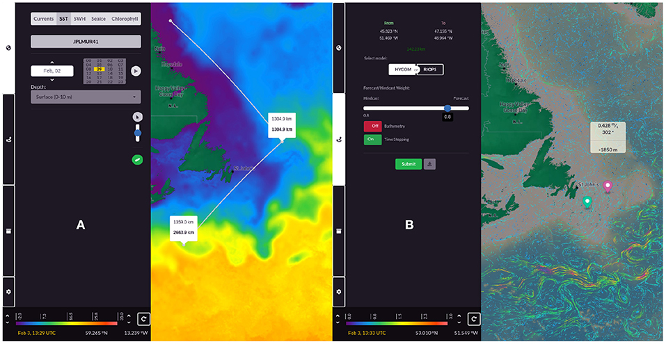
Figure 1. (A) SST layer overlaid by the map distance tool. The left panel shows the user options to change layers, date and time, and depth (if applicable). (B) Screenshot of the cloud-based service v.2.1 showing bathymetry overlaid by the HYCOM model layer. The route–planning panel is shown to the right with user choices such as bathymetry integration.

2.2. Route–Planning Implementation

2.2.1. Ocean Currents

The OceanGNS route–planning module employs a graph search algorithm (Dijkstra, 1959; Wang et al., 2011) to find the optimal path between an AUVs location to a target adapted for ocean current data from a forecasting system such as the HYCOM model. Any other current model or consistent current field data set will work, such as the glider dead reckoned currents themselves populated onto a grid. The route–planning module reduces the current field to within 1.5 the maximum distance to the target that the glider could reach in every direction to arrive at a smaller subset of the full dataset to improve computational speed. The current fields are interpolated onto a local grid points appropriate to the model. Suppose the model resolution is larger than 20% of the distance to the target. In that case, the current field is interpolated using half the native model grid resolution to increase the grid points for the graph searching algorithm to function correctly in situations where higher resolution current data are not available. A model-specific climatology is compiled from previous forecast fields or hindcast results to compute a 7-day running average historical data set for each local grid point to reduce uncertainty in the model forecasts past the daily forecast's 24 h time limit window.

The glider AUV user can represent prior historic and forecast information using a weighted current that represents both sets of data. For each grid point i, the forecast current data C_f(i) and historic data C_h(i) are combined into an effective current—a combination of historical data and the forecast currents (Equation 1). The historic and forecast weights, W_h(i) and W_f(i), are adaptively determined based on the Euclidean distance, L(i), between the grid point and the current position of the glider. The summation of these weights is one. The decaying parameter, a is a constant value that is determined from the forecast period to tune the influence of historical current and the forecast on the effective current and is user-controlled based on prior bias against the forecast data. Figure 2 shows the weight, W_h(i) increases with respect to L(i), while W_f(i) declines.

$\begin{array}{ll}\begin{array}{cc}C(i)& =W_h(i)C_h(i)+W_f(i)C_f(i)\\ W_h(i)& =(e^{(aL(i))}-1)/(1+e^{(aL(i))})\\ W_f(i)& =2/(1+e^{aL(i)})\end{array}& (1)\end{array}$

The different decay parameters will produce different convergence distances. In Figure 2, we show two cases for a = 0.2 and a = 0.1 that represent forecast weightings equivalent to 24–72 h forecast, respectively, resulting in W_(i) decaying toward 0 at 24 and 72 km given an ideal speed of 1 km/h. Therefore, the glider's route–planning beyond the forecast period–depends on the historical averaged current data, C_h(i). The user retains full control of this choice and can set the forecast weight to 1 or 0 depending on the specific navigation situation and the character and quality of available input data

FIGURE 2

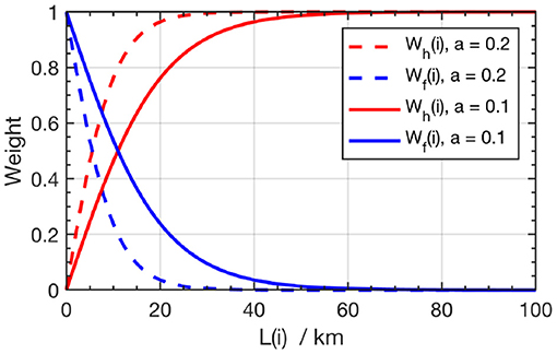
Figure 2. Weight changes over the Euclidean distance at different values of a. When a = 0.2 is tuned for 24-h forecast, as W_f(i) will approach a = 0 at 24 km (equivalent to the 24-h traveling distance of a glider). Likewise, a = 0.1 is tuned for a 72-h forecast.

To determine the optimal path, we compute the moving cost from each grid point to its four adjacent grid points in the north, east, south, and west. For moving from grid point i to j, the time is computed in Equation (2), where α is the apparent angle between the current and the vehicle's moving direction, d is the grid cell size, v_g is the glider speed in still water, ~0.27 m/s (Rudnick et al., 2004). If the apparent current is stronger than v_g, the path is not viable so T(i, j) is set to a large value e.g., 1,000 h.

$\begin{array}{ll}T(i,j)=d/(v_g+0.5(C(i)+C(j))·cos(\alpha ))& (2)\end{array}$

Once OceanGNS has constructed the complete graph that includes all the moving costs from each cell to its neighbor cells, we apply a modified Dijkstra graph search algorithm. Other graphic search algorithms such as A* (Rao and Williams, 2009) could also be incorporated. However, the heuristic function, an estimation of the cost from a grid point to the goal location, is hard to predict due to ocean currents' time-varying nature.

The resultant path determined from the graph search algorithm is further reduced in complexity using a modified 3D Ramer-Douglas-Peucker (RDP) algorithm (Ramer, 1972; Douglas and Peucker, 1973; Zhou et al., 2014). The optimal path computed in the local grid is then translated back to a waypoint list used by the glider for direct navigation or reduced to a heading, depending on the user's needs. Figure 3a shows an example of the OceanGNS path output for a hypothetical trajectory along the Gulf Stream and Figure 3b, back to the start location plotted in python for illustration.

FIGURE 3

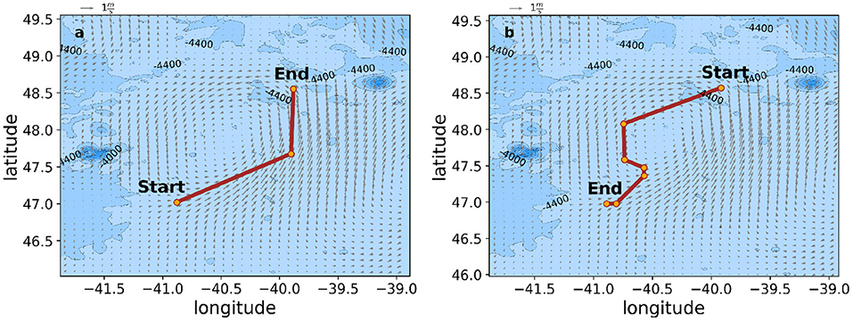
Figure 3. OceanGNS route–planning example for a hypothetical loop mission (a) following along a strong current front and (b) return taking advantage of a return-flowing current to the South-West of the original path.

The forecast's accuracy varies spatially and temporally. We used the averaged current (24 or 72 h) from the forecast model to smooth out noise between timesteps. The glider's path to the target destination is regenerated when the glider surfaces using the up-to-date forecast information as a guide. The daily averaging works in the open ocean, but would probably not be as effective on the continental shelf where tidal currents might dominate. Using such an averaged current ignores high-frequency variability from effects such as inertial or tidal currents. We used the forecast file closest to the dive cycle for one of our experiments in the continental shelf, manually stepping through the available forecast files (see section 3.1) with the algorithm. We are working on integrating a time-varying algorithm into OceanGNS to improve the performance of the route–planning algorithm on the continental shelf. This will be part of the next step in our development and testing of OceanGNS.

2.2.2. Bathymetry Consideration

Frequently, gliders are operated in coastal waters where topography is quote variable and at times very steep. Typically the glider will use the buoyancy pump more frequently in shallow water than when operating in deeper water. While the buoyancy pump will be powered less frequently in deeper water, the instantaneous current draw will increase due to the increased water pressure. Therefore, OceanGNS considers bathymetric data (GEBCO, 2020) during route–planning as an optional constraint to account for the increased power consumption operating in shallow vs. deep water to provide an optimal path considering both time and energy. This feature is particularly useful when piloting a glider from the continental shelf to the deep sea or vice versa.

We found a linear relationship between the current draw and the glider's inflection depth to estimate the current drain when the vehicle is gliding. We applied a linear regression to approximate the current usage during glider inflections. From published glider data (von Oppeln-Bronikowski et al., 2021) we estimate the current draw during gliding (for the Slocum 1000 M G2 glider) is ~0.1 amp. For a diving/climbing cycle, the total battery discharge (in amp-hour) can be calculated (Equation 3), where z is the dive depth, v_z is the vertical speed of the vehicle, I_g is the averaged glider current drain without buoyancy pump activated, I_{c, d} and I_{d, c} are the current draws that can be replaced by the equation estimated from the turnaround time from climbing to diving and vice versa. Similar calculations could be done for other glider types.

$\begin{array}{ll}D(z)=2I_{g}z/v_z+I_{c,d}(z)t_{c,d}+I_{d,c}(z)·t_{d,c}& (3)\end{array}$

The time intervals t_{c, d} and t_{d, c} are the time when the buoyancy pump is active, which is ~150 s for a deep Slocum underwater glider. Different efficiency curves could be implemented and stored depending on the AUV model. During each dive, the forward-moving distance also varies with respect to the diving depth. Assuming the vehicle has an average horizontal speed, v_h of 0.27 m/s. The horizontal traveling distance is L(z) (4) and v_z is the glider vertical speed which is ~0.1 m/s. Using Equations (3) and (4), we compute the ratio of battery discharge and the travel distance (Equation 4). We denote this ratio as the vehicle inefficiency IE(z) (Figure 4), for which z is the depth of the water column at the route–planning grid point.

$\begin{array}{llll}L(z)& =& 2v_{h}z/v_z& (4)\end{array}$

$\begin{array}{llll}IE(z)& =& D(z)/L(z)& (5)\end{array}$

$\begin{array}{llll}{T}^{\prime }(i,j)& =& I{E}^{\prime }(z)T(i,j)& (6)\end{array}$

A glider is more efficient when it dives to the maximum depth possible as part of the mission and requiring less inflections per same travel distance. We modify IE(z) from 4 by setting the minimum inefficiency to 1 at 1,000 m (the maximum diving depth of the glider). We use this modified inefficiency curve IE′(z) in 4 to calculate the final moving cost T′(i, j) for each grid cell with the corrected vehicle inefficiency. The red line in Figure 4 shows the original inefficiency curve calculated from 4. The blue one is the corrected inefficiency IE′(z) curve (Equation 4).

FIGURE 4

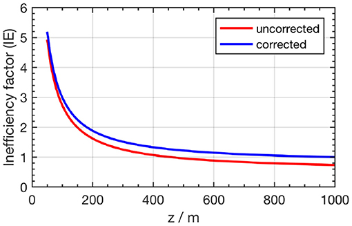
Figure 4. Inefficiency curve before (IE(z): red) and after the correction (IE′(z): blue).

If desired by the glider operator, this moving cost function can be included in the graph constraint for the Dijkstra algorithm inside the main navigation routine. The AUV operators could disable the inefficiency factor in OceanGNS when the glider is flying further offshore with seafloor depths greater than the dive depth. An example of OceanGNS bathymetry considerations is given in Figure 5. The example shows the slightly altered path to take advantage of the deeper water depth while not deviating too much from the most direct path with the most advantageous currents.

FIGURE 5

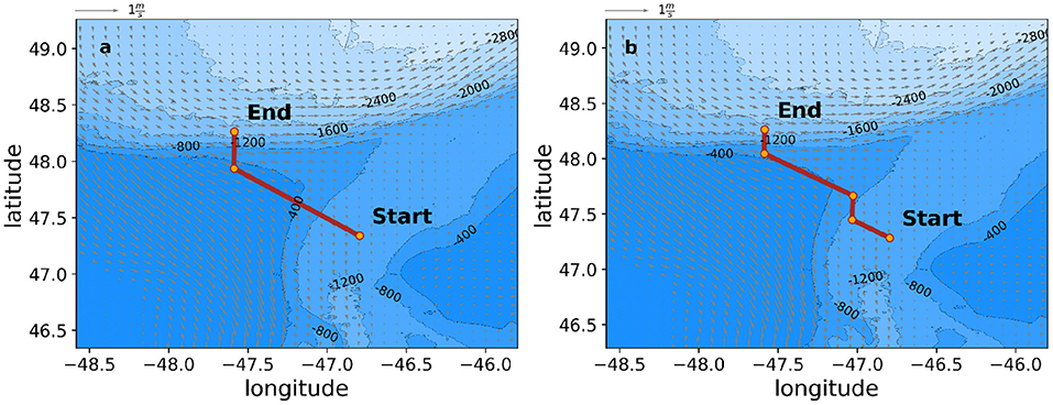
Figure 5. OceanGNS route–planning example for a hypothetical mission passing over a ridge (a) with bathymetry consideration turned off [no IE′(z) considered], and (b) with bathymetry consideration turned on showing the difference in navigation routes under both scenarios.

3. Field Tests

To test the reliability of OceanGNS for piloting and glider mission control, we conducted early field experiments in the Northern Gulf of St. Lawrence (8–15 August 2019) and the Labrador Sea (4 December 2019–27 June 2020). These deployments were not explicitly designed to test OceanGNS in its current state but were used as opportunities for early trials to collect mostly qualitative data. We only tested OceanGNS for a short period in each deployment because we were still actively developing the interface and collecting baseline data to compare results. These tests used the same Slocum G2 Glider “Pearldiver.” The only difference between the deployments was that the glider had an extended bay battery pack during the longer Labrador Sea deployment. Figure 6 shows a summary track map of the two deployments discussed.

FIGURE 6

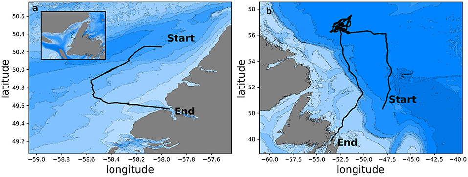
Figure 6. Field Test Cases for OceanGNS. (a) One-week deployment of a glider in the Northern Gulf of St. Lawrence (August 8–15, 2019) from Daniels Harbor to Bonne Bay. (b) Seven-month glider deployment in the Labrador Sea (December 4, 2019 - June 27, 2020). GEBCO bathymetry is shown in the background.

The field deployment tested the algorithm by comparing the waypoints list from OceanGNS to alternate waypoints chosen by the pilot. We evaluate the outcomes of the field trials by calculating the glider speed toward waypoints. From the speed toward waypoints, we compare the speed when using OceanGNS and when not. As a baseline we calculate the ideal speed assuming a constant speed of a glider of 0.27 m/s (at zero current) and add the measured along-track component of the depth-averaged current facing the glider in each dive segment.

$\begin{array}{ll}VI=0.27+Ucos(\theta )& (7)\end{array}$

Equation 7, shows the definition of ideal speed VI that we used in the context of the field tests to evaluate the vehicle speed improvements. Here, U is the along-track component of the depth-averaged current (actual ocean conditions) estimated from the glider data; and θ is the angle between the glider track and the direction of the calculated current U. The dead averaged current from the glider data is estimated based on the difference in intended heading and actual GPS surfacing locations in a full surface to surface cycle (Claus and Bachmayer, 2015). The field tests and chosen methodology is mostly a qualitative analysis and not an ideal evaluation of the merit of the presented tool, and a more careful experiment design can be conducted in the future along a repeat glider observing line.

3.1. Gulf of St. Lawrence Deployment

As part of a project to collect data on the oxygen saturation in the Northern Gulf of St. Lawrence, we deployed a Slocum glider from Daniels Harbor, Newfoundland, with the goal of recovery inside Bonne Bay—a fjord on the West Coast of Newfoundland (see Figure 6). The total distance of the glider track is ~160 km, with large topography changes varying from the deepest of 260–30 m when crossing the shallow sill that divides the mouth of Bonne Bay and Esquiman Channel in the Gulf of St. Lawrence. The glider passed through a strong tidal region, which made navigation from Daniels Harbor to Norris Point difficult. The mission plan was the same throughout the entire deployment which was to pilot the vehicle from the deployment site to Norris Point, Newfoundland.

Active route–planning was used for 2 days (10–12 August 2019) when the glider was in periodic strong head-on currents, which considerably slowed the glider progress. When not using OceanGNS, the pilot choose waypoints in the direction of the target and also based on their perception of the currents from the glider and current maps. We operated the glider in the deep channel across from Bonne Bay's mouth (shallow sill) as the navigation target. The time between glider dive cycles was 4 h.

For this deployment, we used the well established St. Lawrence Global Observatory (SLGO) forecasting system. The SLGO model has a resolution of 0.02° by 0.03° latitude and longitude (Smith et al., 2013). Only surface-level data is available from this model. The model was chosen as it was developed for and tested in the Gulf. The model is run for 48 h allowing forward model time step integration into the route–planning output. We used the SLGO model forecast file closest in time to planned glider dive cycles for which the route planning test were done (e.g., 10–12 August). We picked the individual forecast files and ran the algorithm for 24 h ahead (~25 mission km). To deal with the tidal amplitudes, we did route–planning a couple times a day coinciding with the surfacing of the glider. We kept the glider at the surface (~10 min) while we calculated the next 24 h route plan using the latest available SLGO forecast file for that glider dive cycle. After transmitting the waypoints, the glider dove and we repeated this upon the next surfacing.

We applied the method discussed earlier to evaluate the impact of OceanGNS current-based route–planning on the mission. We calculated the glider speed as the speed toward destination (commanded waypoint). That is the distance traveled between GPS fixes divided by time projected on to the straight line path toward the destination from the previous GPS fix. While using route–planning the pilot experienced a noticeable improvement in the vehicle's performance, making steady progress. In the days before, the glider experienced reduced speeds (0.5 km/h) during parts of the day, significantly increasing the deployment duration. From evaluating the glider data (Figure 7), we see a noticeable difference in glider residual speeds (actual-ideal) while using the route–planning module. Compared with the ideal speed (Equation 7), we find that the glider was 27% faster over that period compared to when the glider was not using OceanGNS.

FIGURE 7

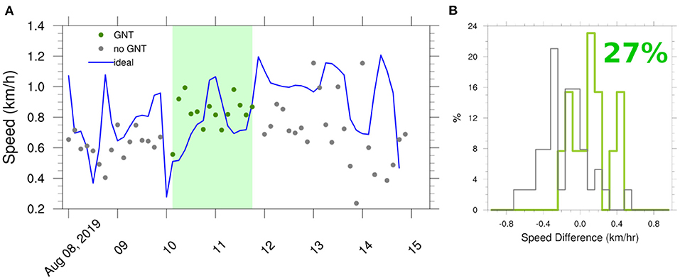
Figure 7. Results of OceanGNS tests for the Gulf of St. Lawrence deployment. (A) Shows the glider speed (dots) toward its intended waypoint (destination) for every dive segment calculated from GPS positions. The green shaded period is the time when OceanGNS was used. The blue line is the calculated ideal speed the glider could achieve based on the constant value of 0.27 m/s and the dead reckoned currents estimated by the glider (Equation 7). (B) Histogram of ideal vs. achieved glider speed toward the target. The residuals of the ideal speed vs. the actual speed toward the waypoint shows that during the OceanGNS test period, the glider speed exceeded the ideal value by an average of 27%.

3.2. Labrador Sea Deployment

We also applied OceanGNS during a long-duration glider deployment in the Labrador Sea from December 4, 2019 to June 27, 2020, a mission to measure heat and gas exchange in the winter. The glider was launched in the Orphan Basin (Figure 6) from the UK research vessel “James Cook” and transited 1,000 km to the central Labrador Sea (de Young et al., 2020). After completing the mission, the glider returned back to Newfoundland following the Labrador Current to speed up the homeward journey. Recovery of the glider was made in Trinity Bay, NL, on June 27, completing the journey after almost 7 months.

For these OceanGNS tests, we used the 1/12° longitude-latitude Hybrid Coordinate Ocean Model—HYCOM (Chassignet et al., 2007) for the route–planning. HYCOM is an assimilative forecast system that produces forecasts for 72 h updated every 24 h with 3 h timesteps. We only included the updated next 24 h forecasts (~50 km) for these tests, and we averaged over 8-time steps to produce a daily averaged ocean current state. We also had the HYCOM hindcast files for the past week with a dynamic weighting (Equation 1) to compensate for the uncertainty in forecasted currents. Depth averaging current was done from 50 to 1,000 m as where the glider spent most of its dive time. The time between surfacings was nearly 11 h on average and covered a distance of 10 km with pitch set to 20°. We did not consider bathymetry during the route–planning periods since the seafloor depth during the experiment is over 1,000 m.

While the glider was sampling in the central Labrador Sea, glider navigation using OceanGNS was not utilized as the vehicle stayed in a small 100 km sampling area and currents were weak. Occasionally sub-mesoscale features (10 km) or larger eddies (30–50 km) would trap the glider and carry it off course. OceanGNS navigation was attempted, but the HYCOM model did not show many of these smaller-scale features the glider experienced. Therefore, navigation during those events was done based on the glider's dead-reckoned currents, steering the glider 90 degrees to get back to the main sampling line. Overall the error between glider dead reckoned currents increased throughout the winter period, starting in January until the return journey in May, which is also the period when the Labrador Sea offers the least data to support the HYCOM assimilation scheme. The disagreement between the actual current circulation and the model output is a limiting factor of OceanGNS (see further discussion in section 4).

From the ideal speed definition (Equation 7) we can compare the glider speed to the waypoint vs the assumed ideal speed and compare the period while using OceanGNS and when not (Figure 8). We quantify the improvement by comparing the residual means during those periods. During the glider track segments that used OceanGNS, we were able to speed up the glider by around 10% (Figure 8B). There are some negative speeds in Figure 8A. These correspond to times when the glider was not making progress toward the target waypoints, for example because of an eddy or a strong adversal current. During the first month of the deployment, the glider covered 1,000 km from the Orphan Basin to the central Labrador Sea. Figure 9 shows good agreement between HYCOM and the glider currents in the first phase of the glider deployment while OceanGNS was used. It also shows an example of route–planning during one of several path-planned segments.

FIGURE 8

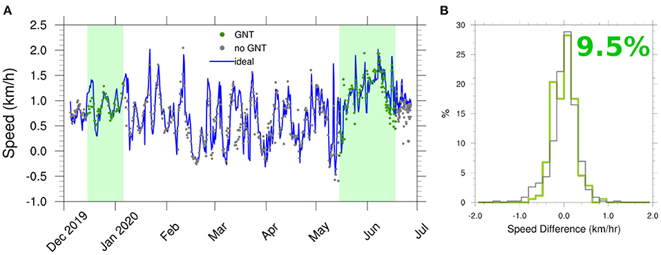
Figure 8. Results of OceanGNS tests for the Labrador Sea mission. (A) Shows the glider speed (dots) toward its intended waypoint (destination) for every dive segment calculated from GPS positions. The shaded period is the time when OceanGNS was used. The blue line is the calculated ideal speed the glider could achieve based on the constant value of 0.27 m/s and the dead reckoned currents estimated by the glider (Equation 7). (B) Histogram of ideal vs. achieved glider speed toward the target. The residuals of the ideal speed vs. the actual speed toward the waypoint shows that during the OceanGNS test period, the glider speed exceeded the ideal value by an average of almost 10%.

FIGURE 9

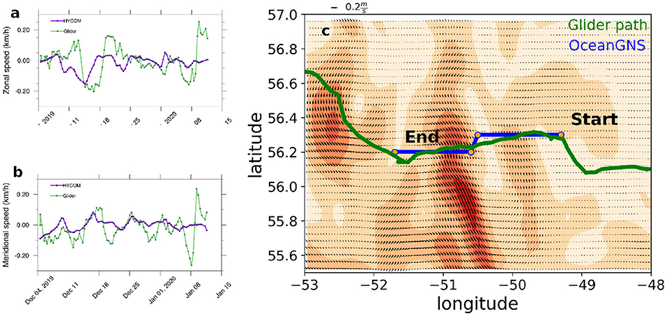
Figure 9. Results of OceanGNS tests for the Labrador Sea. (a,b) Shows the close agreement between glider dead-reckoned currents (u,v component) and the HYCOM model used in these navigation tests. (c) Shows an example from the route–planning done for the mission with the glider track (red) and the planned track (blue) transmitted to the glider from OceanGNS.

4. Discussion

We presented an overview of the tool to support glider mission planning and piloting called OceanGNS. We also presented results from early first field tests of the mission planning software to improve glider control to reach their intended target. We have laid out three criteria that the navigation tool should meet: smartness, reliability and utility. We address these criteria to discuss how OceanGNS meets these requirements and what work is still to be done.

4.1. Performance of OceanGNS

OceanGNS is a tool to improve the whole experience of operating and collecting data with ocean gliders. The focus of the tool is on improving control of the vehicles by predicting the best path to reach a target from various data, including model currents, observations, and the information from the glider itself. The challenge for a navigation system is to supplement or compensate for the uncertainties in ocean model forecasts. OceanGNS does so by respecting a variety of data sources in making a path prediction. It is also flexible and lets the user choose additional constraints such as bathymetry and multiple forecast time segments to make a prediction different than what the default settings would produce. These characteristics point to a tool that is glider–user oriented, adaptable to a wider range of AUV platforms and can reduce the overhead required to currently operate ocean vehicles. What still is missing is the integration of a machine learning algorithm that takes the adjustments from a pilot in route–planning to improve its predictions over time when model performance is low. This would certainly improve the tool, making it smarter with wider user.

The second criteria is the reliability of the system. This has two main components: (1) the tool has to produce route–planning quickly to be useful, and (2) the route–planning has to be at least as good or better than the prediction by the pilot. It should not cause the glider to perform worse - this first point OceanGNS archives with run times of <20 s for most route–planning situations. To achieve the second point in every case is challenging. Still, because the route–planning software is compensated by historical information and the glider information, the risk of a poor route choice is diminished. We evaluated the reliability of the system through field tests within ocean glider deployments moving beyond simulation studies. From these tests, we found a net-benefit to using OceanGNS compared to when not improving the glider speed to the target between 10 and 27% between the deployments. However, these tests are only a first step to evaluate the route–planning module's reliability thoroughly, and dedicated experiments to corroborate results will be required. The system's reliability is also dependent on the availability of reliable input data. In the absence of any information from the glider or from forecast models, climatological datasets, especially in coastal zones, can still dramatically improve the glider utility and progress to reach a target point.

The criteria of utility speaks to the ease with which the tool can help an operator achieve their mission goals. An algorithm can be very good, but hard to use, making it hard to adopt in day-to-day glider activities. The cloud-based interface of OceanGNS with easy access to existing glider software, maps, visualizations, and easy layer integration offers significant support to the pilot. It helps pilots by improving access to information and means less time is spent piecing together information on the ocean environment. All essential ocean information can be presented graphically, quickly, and easily, which also makes OceanGNS a potential tool for education purposes. OceanGNS also allows both interactive and automated piloting with access to manufacturer piloting software. Such is the case for the Slocum glider, allowing them to use autopiloting whereby new route information is given to the glider as frequently as at every surfacing. This could lead to adaptive data-driven sampling (Ferri et al., 2013), whereby glider-OceanGNS automatically adjusts the path to meet the sampling objective and OceanGNS takes over the role of managing multiple vehicles together at the same time. Another direction is goal-driven route–planning (Smedstad et al., 2017) focussing on sampling an ocean region with multiple gliders with specific criteria such as high temporal variability of key ocean variables (e.g., T and S) while minimizing head on currents.

4.2. Implications for Future Missions

The Field trials showed increased glider speed toward the destination of between 9.5 and 27% for the two deployments (Figures 7, 8). We can use the results from the field trials to work out the benefit for two hypothetical scenarios. In the first, a glider is deployed with a single battery pack that can last 30 days and in the second the glider is deployed with a larger battery pack that can last for 180 days on a long mission. An average speed of 0.27 m/s which works out to 22 km a day for a glider that is moving at speed 95% of the time (excludes times spent at the surface). Over 30 days that is 665 km or for 180 days, roughly 4,000 km. Using OceanGNS the glider speed toward the target is improved on average by 18.5%. This translates into increasing the mean glider speed from 0.27 to 0.32 m/s or 26 km per day. This speed improvement increases the range of the glider by 123 km for a 30 day deployment or 728 km for a 180 day deployment.

On the other hand, the goal of route–planning might not be to increase the range of the deployment but to increase the number of observations along a fixed track length. For a hypothetical track of 250 km a glider going 0.27 m/s, 95% of the day can manage to complete the track in <11.3 days on average. Using this number a 30 day deployment of a glider could yield 2.7 passes of this track. With OceanGNS the glider completes the track in 9.5 days and can complete 3.2 passes in 30 days. Over 180 days that would be an advantage of an extra 3 completed passes of the 250 km track. Care must be taken to ensure that the route plan does not cause the glider to deviate from the track. A corridor mode could be implemented into the algorithm by setting the cost of grid points prohibitively high past a certain distance from the intended track. This would cause the algorithm to find the best path within a defined corridor of a certain width and ensure that tracks are comparable between transects. This work is in development and should be ready in the near future.

Another consideration is that if other factors are fixed (deployment duration, number of glider passes) we can work out the battery savings. This analysis becomes more applicable if the goal of a glider deployment is not to just sample one mission, but to be redeployed multiple times in a given year. The need for this could arise for example from the expense associated with battery replacements. Using OceanGNS the glider can complete the full pass to and back in 19 days with 11 days of sampling left to spare vs. 7.4 days without OceanGNS. This means a battery cost efficiency increase of 32%. For a large lithium battery pack this might be very attractive given that the glider can now be redeployed more times on a single battery, accomplishing more missions. This analysis is based on idealized scenarios. However, the mean glider speed values are on average in agreement with the real glider performance reported in the literature. More tests are required to further capture the result we have shown, but so far the benefits of OceanGNS look very promising for glider operators.

4.3. Limitations and Solutions

OceanGNS performed remarkably well in the field tests discussed. The tool can simplify decision-making around glider navigation and coordinate deployments from multiple glider platforms. Indeed, this tool meets the smart, reliable and utility requirements to a large degree. Improvements will further enhance the tool. However, some limitations of the current technology require more work. The largest limiting factor is the input current model. The slow speed of gliders (typically 0.2–0.3 m/s) requires high-resolution ocean forecast models initialized with sufficient observations to represent the small scale current features important to glider operations. This limitation is not unique to our approach. Improvements in temporal and spatial coverage of observations are needed to define ocean features at the required scales to improve model forecasts (Fox-Kemper et al., 2019). For each deployment, it will be necessary to determine which model is most valuable and the limitations, perhaps seasonal, or perhaps location, of the model. In general the model will improve as more real-time data is incorporated into the model, perhaps from satellites, Argo floats, or gliders. Ensemble models can help to reduce some of the uncertainty inherent with a single model prediction, but this is not universally true (Weigel et al., 2008). For example, some of the operational models used for iceberg forecasting use small ensemble of models for operational use, although there are some studies that have suggested ensemble forecasting did not yield improvements in forecast skill (Allison et al., 2014) or only under certain conditions (Kielley, 2020). Thus, it remains true that under certain circumstances the input of the pilot will be required. The direct current measurements offered by the gliders, permit real-time assessment of the utility of the model data and thus the performance of OceanGNS.

To overcome some of these challenges we also need to consider other techniques. One idea briefly mentioned earlier in the introductory sections would be supervised machine learning algorithms to take advantage of pilot expert knowledge when paths are modified. The objective of such an algorithm would be to compute a range of possible paths based on different inputs to the route–planner. The algorithm would learn from the pilot's choices regarding model selection, route constraints and the time when route planning was most requested. An initial step into automating route–planning criteria could be to use the glider velocities to determine the model forecast skill over the past few glider segments. OceanGNS could use the results to decide if it should give more weight to climatological data or the forecast system. However, glider dead-reckoned currents are not perfect themselves being an average over sometimes a large distance (typically several kilometers). They are also delayed for the previous dive cycle and may not be valid for the next segment. Over time, a more advanced algorithm using multiple datasets based on assembled information from ocean models, glider data, in-situ glider measurements, and pilot inputs could help minimize the negative impact of a single approach against another. Neural networks could capture such nuances in the data but require massive training data to avoid over or underfitting the data. More conversations on this level have to happen to identify a robust methodology to capture pilot skills in route–planning to overcome the limitations of ocean forecast models.

Another solution to the modeling problem could be to develop regional best practices around using different regional models (e.g., NCOM, WMOP, NGOFS etc). Our test results so far only apply to a small geographic area and a small number of ocean forecast models (SLGO, HYCOM, RIOPS, CMEMS, and WMOP model). We are working on implementing more models so that several different models could be tested during a deployment. Over time glider groups could explore models suitable for their operations and inform the glider community of their experience. For example, we note that HYCOM showed good agreement during the initial phase of the Labrador Sea deployment, but over time the error increased. Such knowledge could help decide how and which data sets to use in decision making around flying gliders. The Mediterranean glider group at SOCIB (www.www.socib.es) have also looked at model and glider comparisons (Juza et al., 2016; Mendiondo et al., 2020). Published literature and studies would inform the strategy and experimental setup behind new navigation tests. More formally, we are working on implementing a path-planning confidence score based on calculating the routes from all implemented model time steps using different averaging of forecast steps and algorithm settings (e.g., bathymetry on or off, different glider speeds etc). The runs would produce different paths. If convergence of paths is achieved the pilot could be given visual feedback. In contrast, if the spread in predictions is high, then the pilot can be warned by the system that confidence is low. In addition as the mission progresses the data from the glider can be used to back-calculate which models are performing best and give the pilot feedback on the overall performance of OceanGNS.

An increase in the number of users applying tools such as OceanGNS would help us understand the benefits and limitations of different approaches to planning glider missions. We are just one of many groups that operate gliders (see Testor et al., 2019). By making this tool cloud-based, easy to access and providing integration possibilities into existing systems through an API, we have paved the start for a new way to do ocean glider mission planning. However, we need the input from the wider glider community to improve the capabilities of OceanGNS.

5. Summary and Future Development

Ocean gliders are frequently used to close observing gaps by traditional remote sensing platforms. They have increased in numbers and are becoming a mature technology (Testor et al., 2010, 2019). Differences across glider platforms are minimal and three dominant manufacturers exist whose platforms are utilized to varying degrees around the world. It is time to improve the synthesis of different platforms to coordinate these platforms better. This new glider navigation tool—OceanGNS—offers a significant improvement for glider navigation and coordination of different glider platforms. OceanGNS can improve the speed of gliders and can do so operationally for many vehicles at a time. We provided an overview of the tool, its many capabilities and demonstrated the utility through initial field deployments using Slocum gliders. These tests show that OceanGNS did demonstrably improve glider navigation toward its target, speeding up the journey and extending battery range. We also further discussed the importance of these results through common operational scenarios. Through these exercises we further demonstrate the usefulness of OceanGNS to operational glider sampling.

We evaluated the tool against three criteria: intelligence, reliability, and utility and demonstrated that it meets each of these criteria to varying degrees. This technology is at an early stage of development and significant improvements and more testing are needed. Particularly the time–varying algorithm is something we are developing and need to test. The algorithm used could be improved in several ways. The graph search could be refined to include more discrete quadrants. At the moment, the algorithm only chooses between four directions (N, S, E, W). In addition machine learning algorithms could be included to learn from pilot input and correct for gaps in model forecasting skills. We are working to add features to use the glider data to assess model performance and compare the effectiveness of different models. The other issue around user adoption could resolve gaps in models by yielding best practices on how to gain the most from models to improve gliders' navigation. These best practices could be as direct as specifying which model is best for a particular region or could provide at least more insight into the model accuracy for particular missions. There is also the opportunity to learn and the strengths and weaknesses of different models.

Another advantage of this tool is that it is not restricted to a particular glider platform. There are now many different types of gliders being used by a growing glider community. Indeed any glider manufacturer or user could use this tool. The benefit would be the possibility for a swarm concept implementation across different platforms, whereby the glider mission is coordinated between the different gliders using OceanGNS. The navigation strategy could be used to keep the gliders from diverging too much from each other and sampling coordinated across a common strategy.

Data Availability Statement

Glider data has been archived on SEANOE (https://www.seanoe.org/data/00681/79349/).

Author Contributions

All authors contributed to the ideas and implementation of OceanGNS. NvOB initiated the manuscript and carried out the glider deployments and together with MZ. TB and BY analyzed deployment results. MZ initiated the OceanGNS prototype and TB implemented OceanGNS in its current form. BY carried out early work on glider navigation, conceived the ideas, and contributed to the design of OceanGNS. All authors contributed to the manuscript, revisions, and provided constructive input throughout the revisions.

Funding

We gratefully acknowledge funding for this work, which has been enabled by the Ocean Frontier Institute's Module O Theme: Transforming Ocean Observations.

Conflict of Interest

The authors declare that the research was conducted in the absence of any commercial or financial relationships that could be construed as a potential conflict of interest.

The handling editor declared a past co-authorship with one of the authors BY.

Publisher's Note

All claims expressed in this article are solely those of the authors and do not necessarily represent those of their affiliated organizations, or those of the publisher, the editors and the reviewers. Any product that may be evaluated in this article, or claim that may be made by its manufacturer, is not guaranteed or endorsed by the publisher.

Acknowledgments

We thank Mark Downey for field work support. We acknowledge the support of Fisheries and Oceans Canada as part of the James Cook cruise in December 2019, that allowed us to deploy the glider offshore. The field deployment activity was supported by the Ocean Frontier Institute (OFI) and the Natural Sciences and Engineering Research Council (NSERC). MZ's expenses for the deployment were partially supported by the Graduate School of Oceanography, University of Rhode Island.

References

Allison, K., Crocker, G., Tran, H., and Carrieres, T. (2014). An ensemble forecast model of iceberg drift. Cold Reg. Sci. Technol. 108, 1–9. doi: 10.1016/j.coldregions.2014.08.007

CrossRef Full Text | Google Scholar

Alvarez, A., Caiti, A., and Onken, R. (2004). Evolutionary path planning for autonomous underwater vehicles in a variable ocean. IEEE J. Ocean. Eng. 29, 418–429. doi: 10.1109/JOE.2004.827837

PubMed Abstract | CrossRef Full Text | Google Scholar

Capet, A., Fernández, V., She, J., Dabrowski, T., Umgiesser, G., Staneva, J., et al. (2020). Operational modeling capacity in European seas-an EuroGOOS perspective and recommendations for improvement. Front. Mar. Sci. 7:129. doi: 10.3389/fmars.2020.00129

CrossRef Full Text | Google Scholar

Chassignet, E. P., Hurlburt, H. E., Smedstad, O. M., Halliwell, G. R., Hogan, P. J., Wallcraft, A. J., et al. (2007). The HYCOM (hybrid coordinate ocean model) data assimilative system. J. Mar. Syst. 65, 60–83. doi: 10.1016/j.jmarsys.2005.09.016

CrossRef Full Text | Google Scholar

Claus, B., and Bachmayer, R. (2015). Terrain-aided navigation for an underwater glider. J. Field Robot. 32, 935–951. doi: 10.1002/rob.21563

PubMed Abstract | CrossRef Full Text | Google Scholar

Claus, B., Bachmayer, R., and Williams, C. D. (2010). Development of an auxiliary propulsion module for an autonomous underwater glider. Proc. Instit. Mech. Eng. Part M 224, 255–266. doi: 10.1243/14750902JEME204

CrossRef Full Text | Google Scholar

Davis, R. E., Eriksen, C. C., and Jones, C. P. (2002). “Autonomous buoyancy-driven underwater gliders,” in The Technology and Applications of Autonomous Underwater Vehicles (London), 37–58. doi: 10.1201/9780203522301.ch3

PubMed Abstract | CrossRef Full Text | Google Scholar

Davis, R. E., Talley, L. D., Roemmich, D., Owens, W. B., Rudnick, D. L., Toole, J., et al. (2019). 100 years of progress in ocean observing systems. Meteorol. Monogr. 59, 3.1–3.46. doi: 10.1175/AMSMONOGRAPHS-D-18-0014.1

CrossRef Full Text | Google Scholar

de Young, B., Frajka-Williams, E., von Oppeln-Bronikowski, N., and Woodward, S. (2020). Technicalities: exploring the Labrador sea with autonomous vehicles. J. Ocean Technol. 15, 134–139.

Google Scholar

Dijkstra, E. W. (1959). A note on two problems in connexion with graphs. Numer. Math. 1, 269–271. doi: 10.1007/BF01386390

CrossRef Full Text | Google Scholar

Douglas, D. H., and Peucker, T. K. (1973). Algorithms for the reduction of the number of points required to represent a digitized line or its caricature. Cartographica 10, 112–122. doi: 10.3138/FM57-6770-U75U-7727

CrossRef Full Text | Google Scholar

Eichhorn, M., Williams, C. D., Bachmayer, R., and de Young, B. (2010). “A mission planning system for the AUV ‘SLOCUM Glider' for the Newfoundland and Labrador shelf,” in OCEANS'10 IEEE Sydney (Sydney), 1–9. doi: 10.1109/OCEANSSYD.2010.5603919

PubMed Abstract | CrossRef Full Text | Google Scholar

Ferri, G., Cococcioni, M., and Alvarez, A. (2013). “Sampling on-demand with fleets of underwater gliders,” in 2013 MTS/IEEE OCEANS Bergen (Bergen), 1–9. doi: 10.1109/OCEANS-Bergen.2013.6608037

PubMed Abstract | CrossRef Full Text | Google Scholar

Fiorelli, E., Leonard, N. E., Bhatta, P., Paley, D. A., Bachmayer, R., and Fratantoni, D. M. (2006). Multi-AUV control and adaptive sampling in Monterey Bay. IEEE J. Ocean. Eng. 31, 935–948. doi: 10.1109/JOE.2006.880429

PubMed Abstract | CrossRef Full Text | Google Scholar

Fox-Kemper, B., Adcroft, A., Böning, C. W., Chassignet, E. P., Curchitser, E., Danabasoglu, G., et al. (2019). Challenges and prospects in ocean circulation models. Front. Mar. Sci. 6:65. doi: 10.3389/fmars.2019.00065

CrossRef Full Text | Google Scholar

Fujii, Y., Rémy, E., Zuo, H., Oke, P., Halliwell, G., Gasparin, F., et al. (2019). Observing system evaluation based on ocean data assimilation and prediction systems: on-going challenges and a future vision for designing and supporting ocean observational networks. Front. Mar. Sci. 6:417. doi: 10.3389/fmars.2019.00417

CrossRef Full Text | Google Scholar

GEBCO (2020). The GEBCO 2020 Grid-A Continuous Terrain Model of the Global Oceans and Land. GEBCO.

Google Scholar

Huynh, V. T., Dunbabin, M., and Smith, R. N. (2015). “Predictive motion planning for AUVs subject to strong time-varying currents and forecasting uncertainties,” in 2015 IEEE International Conference on Robotics and Automation (ICRA) (Seattle, WA), 1144–1151. doi: 10.1109/ICRA.2015.7139335

PubMed Abstract | CrossRef Full Text | Google Scholar

Juza, M., Mourre, B., Renault, L., Gómara, S., Sebastián, K., Lora, S., et al. (2016). SOCIB operational ocean forecasting system and multi-platform validation in the Western Mediterranean Sea. J. Oper. Oceanogr. 9, 155–166. doi: 10.1080/1755876X.2015.1117764

CrossRef Full Text | Google Scholar

Kielley, E. (2020). Iceberg drift ensemble forecasting (Master's thesis). Memorial University of Newfoundland and Labrador, St. John's, NL, Canada.

Google Scholar

Kularatne, D., Bhattacharya, S., and Hsieh, M. A. (2016). “Time and energy optimal path planning in general flows,” in Robotics: Science and Systems (Ann Arbor, MI), 1–10.

Google Scholar

Lellouche, J.-M., Greiner, E., Le Galloudec, O., Garric, G., Regnier, C., Drevillon, M., et al. (2018). Recent updates to the Copernicus Marine Service global ocean monitoring and forecasting real-time 1/12° high-resolution system. Ocean Sci. 14, 1093–1126. doi: 10.5194/os-14-1093-2018

CrossRef Full Text | Google Scholar

Leonard, N. E., Paley, D. A., Davis, R. E., Fratantoni, D. M., Lekien, F., and Zhang, F. (2010). Coordinated control of an underwater glider fleet in an adaptive ocean sampling field experiment in Monterey Bay. J. Field Robot. 27, 718–740. doi: 10.1002/rob.20366

PubMed Abstract | CrossRef Full Text | Google Scholar

Liblik, T., Karstensen, J., Testor, P., Alenius, P., Hayes, D., Ruiz, S., et al. (2016). Potential for an underwater glider component as part of the Global Ocean Observing System. Methods Oceanogr. 17, 50–82. doi: 10.1016/j.mio.2016.05.001

CrossRef Full Text | Google Scholar

Lolla, T., Lermusiaux, P. F. J., Ueckermann, M. P., and Haley, P. J. (2014). Time-optimal path planning in dynamic flows using level set equations: theory and schemes. Ocean Dyn. 64, 1373–1397. doi: 10.1007/s10236-014-0757-y

CrossRef Full Text | Google Scholar

Lucas, C., Hernández-Sosa, D., Greiner, D., Zamuda, A., and Caldeira, R. (2019). An approach to multi-objective path planning optimization for underwater gliders. Sensors 19:24. doi: 10.3390/s19245506

PubMed Abstract | CrossRef Full Text | Google Scholar

Mendiondo, K., Mestas-Nunez, A., de Fommervault, O. P., and Xie, H. (2020). “Buoyancy glider observations of current velocities in the Northwestern Mediterranean sea during April 2018,” in Earth and Space Science Open Archive ESSOAr (San Francisco, CA). doi: 10.1002/essoar.10502594.1

PubMed Abstract | CrossRef Full Text | Google Scholar

Merckelbach, L. (2013). On the probability of underwater glider loss due to collision with a ship. J. Mar. Sci. Technol. 18, 75–86. doi: 10.1007/s00773-012-0189-7

CrossRef Full Text | Google Scholar

Petillo, S., Schmidt, H., Lermusiaux, P., Yoerger, D., and Balasuriya, A. (2015). “Autonomous & adaptive oceanographic front tracking on board autonomous underwater vehicles,” in OCEANS 2015 Genova (Genova), 1–10. doi: 10.1109/OCEANS-Genova.2015.7271616

PubMed Abstract | CrossRef Full Text | Google Scholar

Ramer, U. (1972). An iterative procedure for the polygonal approximation of plane curves. Comput. Graph. Image Process. 1, 244–256. doi: 10.1016/S0146-664X(72)80017-0

CrossRef Full Text | Google Scholar

Ramos, A., García-Garrido, V., Mancho, A., Wiggins, S., Coca, J., Glenn, S., et al. (2018). Lagrangian coherent structure assisted path planning for transoceanic autonomous underwater vehicle missions. Sci. Rep. 8, 1–9. doi: 10.1038/s41598-018-23028-8

PubMed Abstract | CrossRef Full Text | Google Scholar

Rao, D., and Williams, S. B. (2009). “Large-scale path planning for underwater gliders in ocean currents,” in Australasian Conference on Robotics and Automation (Sydney), 2–4.

Google Scholar

Roemmich, D., Johnson, G. C., Riser, S., Davis, R., Gilson, J., Owens, W. B., et al. (2009). The argo program: observing the global ocean with profiling floats. Oceanography 22, 34–43. doi: 10.5670/oceanog.2009.36

CrossRef Full Text | Google Scholar

Rudnick, D. L. (2016). Ocean research enabled by underwater gliders. Annu. Rev. Mar. Sci. 8, 519–541. doi: 10.1146/annurev-marine-122414-033913

PubMed Abstract | CrossRef Full Text | Google Scholar

Rudnick, D. L., Davis, R. E., Eriksen, C. C., Fratantoni, D. M., and Perry, M. J. (2004). Underwater gliders for ocean research. Mar. Technol. Soc. J. 38, 73–84. doi: 10.4031/002533204787522703

CrossRef Full Text | Google Scholar

Smedstad, L. F., Barron, C. N., Book, J. W., Osborne, J. J., Souopgui, I., Rice, A. E., et al. (2017). “An updated system for guidance of heterogeneous platforms used for multiple gliders in a real-time experiment,” in American Geophysical Union, Fall Meeting 2017 (New Orleans, LA).

Google Scholar

Smith, G. C., Roy, F., and Brasnett, B. (2013). Evaluation of an operational ice-ocean analysis and forecasting system for the Gulf of St Lawrence. Quart. J. R. Meteorol. Soc. 139, 419–433. doi: 10.1002/qj.1982

PubMed Abstract | CrossRef Full Text | Google Scholar

Smith, R. N., Chao, Y., Li, P. P., Caron, D. A., Jones, B. H., and Sukhatme, G. S. (2010). Planning and implementing trajectories for autonomous underwater vehicles to track evolving ocean processes based on predictions from a regional ocean model. Int. J. Robot. Res. 29, 1475–1497. doi: 10.1177/0278364910377243

CrossRef Full Text | Google Scholar

Subramani, D. N., and Haley, P. J. Jr, Lermusiaux, P. F. (2017). Energy-optimal path planning in the coastal ocean. J. Geophys. Res. 122, 3981–4003. doi: 10.1002/2016JC012231

PubMed Abstract | CrossRef Full Text | Google Scholar

Testor, P., de Young, B., Rudnick, D. L., Glenn, S., Hayes, D., Lee, C. M., et al. (2019). Oceangliders: a component of the integrated goos. Front. Mar. Sci. 6, 422.1–422.32. doi: 10.3389/fmars.2019.00422

CrossRef Full Text | Google Scholar

Testor, P., Meyers, G., Pattiaratchi, C., Bachmayer, R., Hayes, D., Pouliquen, S., et al. (2010). “Gliders as a component of future observing systems,” in Proceedings of OceanObs'09: Sustained Ocean Observations and Information for Society Conference (Venice), 1–18.

Google Scholar

Thompson, D. R., Chien, S., Chao, Y., Li, P., Cahill, B., Levin, J., et al. (2010). “Spatiotemporal path planning in strong, dynamic, uncertain currents,” in 2010 IEEE International Conference on Robotics and Automation (Anchorage, AK), 4778–4783. doi: 10.1109/ROBOT.2010.5509249

PubMed Abstract | CrossRef Full Text | Google Scholar

von Oppeln-Bronikowski, N., de Young, B., Bachmayer, R., Palter, J., Claus, B., Zhou, M, et al. (2021). Memorial University Ocean Glider Deployments: 2005—Present. Available online at: https://www.seanoe.org/data/00681/79349/

Google Scholar

Wang, H., Yu, Y., and Yuan, Q. (2011). “Application of Dijkstra algorithm in robot path-planning,” in 2011 Second International Conference on Mechanic Automation and Control Engineering (Inner Mongolia), 1067–1069.

Google Scholar

Weigel, A. P., Liniger, M. A., and Appenzeller, C. (2008). Can multi-model combination really enhance the prediction skill of probabilistic ensemble forecasts? Q. J. R. Meteorol. Soc. 134, 241–260. doi: 10.1002/qj.210

CrossRef Full Text | Google Scholar

Zamuda, A., and Sosa, J. D. H. (2019). Success history applied to expert system for underwater glider path planning using differential evolution. Expert Syst. Appl. 119, 155–170. doi: 10.1016/j.eswa.2018.10.048

CrossRef Full Text | Google Scholar

Zeng, Z., Lian, L., Sammut, K., He, F., Tang, Y., and Lammas, A. (2015). A survey on path planning for persistent autonomy of autonomous underwater vehicles. Ocean Eng. 110, 303–313. doi: 10.1016/j.oceaneng.2015.10.007

CrossRef Full Text | Google Scholar

Zeng, Z., Sammut, K., Lian, L., He, F., Lammas, A., and Tang, Y. (2016). A comparison of optimization techniques for AUV path planning in environments with ocean currents. Robot. Auton. Syst. 82, 61–72. doi: 10.1016/j.robot.2016.03.011

CrossRef Full Text | Google Scholar

Zhou, M., Bachmayer, R., and de Young, B. (2014). “Initial performance analysis on underside iceberg profiling with autonomous underwater vehicle,” in 2014 Oceans St. John's (St. John's, NL), 1–6. doi: 10.1109/OCEANS.2014.7003239

PubMed Abstract | CrossRef Full Text | Google Scholar