Pathways, Volume Transport, and Seasonal Variability of the Lower Deep Limb of the Pacific Meridional Overturning Circulation at the Yap-Mariana Junction

Introduction

The deep and bottom waters of the North Pacific Ocean have their origins in Antarctic and are carried by the northward lower deep branch of the Pacific Meridional Overturning Circulation (L-PMOC), also referred to as the Pacific Deep Western Boundary Current. Therefore, the L-PMOC impacts the transport and residence time of heat and carbon and plays an essential role in the global climate change (Johnson et al., 2007). However, observations in the deep layers are still limited, and large gaps remain in our knowledge of the L-PMOC pathways, mixing, and variability.

The general route of the L-PMOC has been inferred based on previous mooring and hydrography measurements (Figure 1). North of the mid-latitudes in the South Pacific, the L-PMOC layer corresponds to potential temperatures θ < 1.2°C and depths greater than ∼3,500 m (Kawabe et al., 2006, 2009). The L-PMOC separates from the Antarctic Circumpolar Current (ACC) and flows northward to the east of New Zealand and the Tonga-Kermadec Ridge (Whitworth et al., 1999) and then through the Samoan Passage (Rudnick, 1997; Voet et al., 2015) or around the Manihiki Plateau (Pratt et al., 2019). The L-PMOC continues northward and enters the Central Pacific Basin and bifurcates into the eastern and western branches (Johnson and Toole, 1993; Kawabe et al., 2003, 2006). The western branch passes through the Melanesian and East Mariana Basins (EMBs) and finally arrives at the Yap-Mariana Junction (YMJ) deep channels. However, its pathway after passing the YMJ is largely unknown. The L-PMOC carries the Lower Circumpolar Water (LCPW), which originates from the Southern Ocean (Callahan, 1972; Mantyla and Reid, 1983) and is characterized by a salinity maximum and a silica minimum (Johnson and Toole, 1993). Above the L-PMOC lies the upper deep branch of the PMOC (U-PMOC), which extends over a depth of ∼2,000–3,500 m. This layer also originates from the Southern Ocean but can arrive at the YMJ through a different route from the L-PMOC (Kawabe et al., 2003; Kawabe and Fujio, 2010; Wang et al., 2020). The U-PMOC carries the Upper Circumpolar Water (UCPW), which is relatively warm, fresh, oxygen-poor, and silica-rich compared to the LCPW (Kawabe et al., 2006; Kawabe and Fujio, 2010).

FIGURE 1

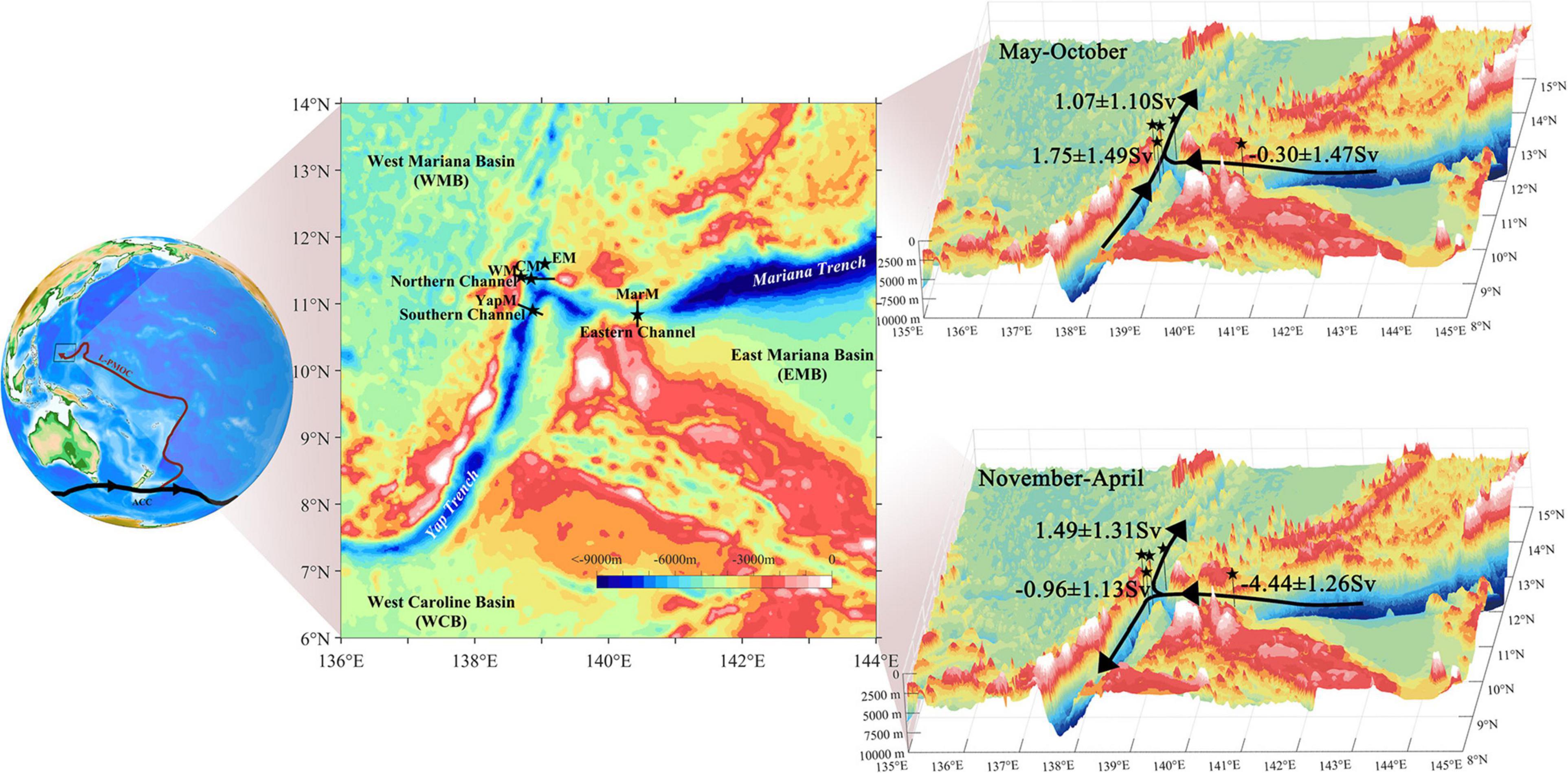
Figure 1. (Left) Schematic flow pattern of lower deep branch of the Pacific Meridional Overturning Circulation (L-PMOC) from the Antarctic Circumpolar Current (ACC) to the western Pacific (after Siedler et al., 2004; Kawabe and Fujio, 2010). (Middle) Map of topography near the Yap-Mariana Junction showing locations of five moorings MarM, YapM, WM, CM, and EM (stars) and the cross sections of Eastern, Southern, and Northern Channels (lines). (Right) The seasonal pathways (arrows) and volume transports (numbers: mean ± standard deviation) of the L-PMOC during (right upper) May–October and (right lower) November–April are given based on the present study. Stars denote the mooring locations. The bathymetry is from ETOPO1.

The YMJ is a major gateway for the L-PMOC flowing into the Western Pacific Ocean (WPO). We refer to the Philippine Sea and the West and East Caroline Basins, which are separated from the North Pacific by tall ridges, as WPO. The natural geographic constraint of the YMJ deep channel makes it a more convenient site for monitoring the variability of the L-PMOC. The site marks the junction of three deep channels: the Eastern Channel connecting to the Mariana Trench and the EMB, the Southern Channel connecting to the Yap Trench and the West Caroline Basin (WCB), and the Northern Channel connecting to the West Mariana Basin (WMB) (Figure 1). At the YMJ, Siedler et al. (2004) first presented the characteristics of the L-PMOC based on moored current meters deployed on the western side of the Northern Channel from October 1996 to March 1998. The L-PMOC was directed northward with a mean speed of 10.4 cm s^–1 at 4,220 m. By combining data from Siedler et al. (2004) with new mooring observations on the western and eastern sides of the Northern Channel during 2014–2017, Wang et al. (2020) first revealed the seasonal variability of the L-PMOC and U-PMOC. During December–May, the L-PMOC flows northward at depths below ∼3,800 m with a speed exceeding 20 cm s^–1 on the western side and is accompanied by a weaker southward return flow on the eastern side. During June–November, the L-PMOC becomes very weak, and the U-PMOC intensifies and flows southward at depths over ∼3,000–3,800 m on the eastern side of the channel. Analysis of the hydrography features suggested that before arriving at the Northern Channel, the U-PMOC intrudes into the WMB mainly through a shallower deep channel northeast of the Northern Channel after arriving at the Mariana Trench. The seasonal variations of the L-PMOC and U-PMOC are accompanied by geostrophically balanced seasonal intrusions of the LCPW and UCPW.

The lack of simultaneous observations in the three channels that meet at the YMJ has hindered our understanding of the distribution and variability of LCPW transport in the channels, key features in the climatologically important deep and bottom circulation in the WPO. To make progress on this topic, we deployed five moorings from 2018 to 2019 in the three channels mentioned above. The analysis of the observational result is first presented, and the underlying dynamics are explored through the analysis of the solution of a high-resolution numerical ocean model.

Data

Mooring Data

As a part of the Scientific Observing Network of the Chinese Academy of Sciences (CASSON), one mooring was deployed in the Eastern Channel close to the Mariana Trench (hereafter referred to as MarM), one mooring deployed in the Southern Channel close to the Yap Trench (YapM), and three subsurface moorings deployed on the western, central, and eastern sides of the Northern Channel (WM, CM, and EM), respectively (black stars in the middle panel of Figure 1). The longitudes/latitudes and durations of MarM, YapM, WM, CM, and EM are 140.43°E/10.84°N from December 12, 2018 to December 24, 2019, 138.87°E/10.90°N from December 11, 2018 to December 25, 2019, 138.69°E/11.40°N from January 26 to December 26, 2019, 138.84°E/11.37°N from January 24 to December 25, 2019, and 139.05°E/11.60°N from January 23 to December 26, 2019, respectively. Each mooring was equipped with five to seven discrete Nortek Aquadopp deep current meters, and seven to 11 discrete SBE37-SM conductivity–temperature–depth (CTD) or RBR solo temperature (T) sensors between 3,000 m and the bottom. The detailed configurations of the mooring measurement are given in Table 1. Current meters measured point velocity in the deep layers hourly. The CTDs returned records of temperature, salinity, and pressure every 10 min. The Ts sampled temperature every 10 min. The measurement depths of Ts are obtained using the recorded depths of CTDs and the nominal separation depths between Ts and adjacent CTDs. The potential temperature corresponding to a measured T is derived using the salinity value from the CTD cast carried out during the mooring deployment. All data are low-pass filtered with a 72-h Lanczos filter to remove the effects of inertial fluctuations and tides and then averaged to derive the daily means. Velocity vectors were rotated to the along- and cross-channel directions (x and y axes) with positive x toward 90° (clockwise from north orientation, the same hereinafter) in the Eastern Channel, 23.25° in the Southern Channel, and 0° in the Northern Channel, respectively. The cross-channel section along the y-axis in each channel is denoted by a black line in the middle panel of Figure 1. In the Northern Channel, we assume that the observed along-channel velocities from the three moorings represent the flow across the section of 11.37°N, although their latitudes are slightly different. Velocity and temperature data were then interpolated vertically to 1-m intervals.

TABLE 1

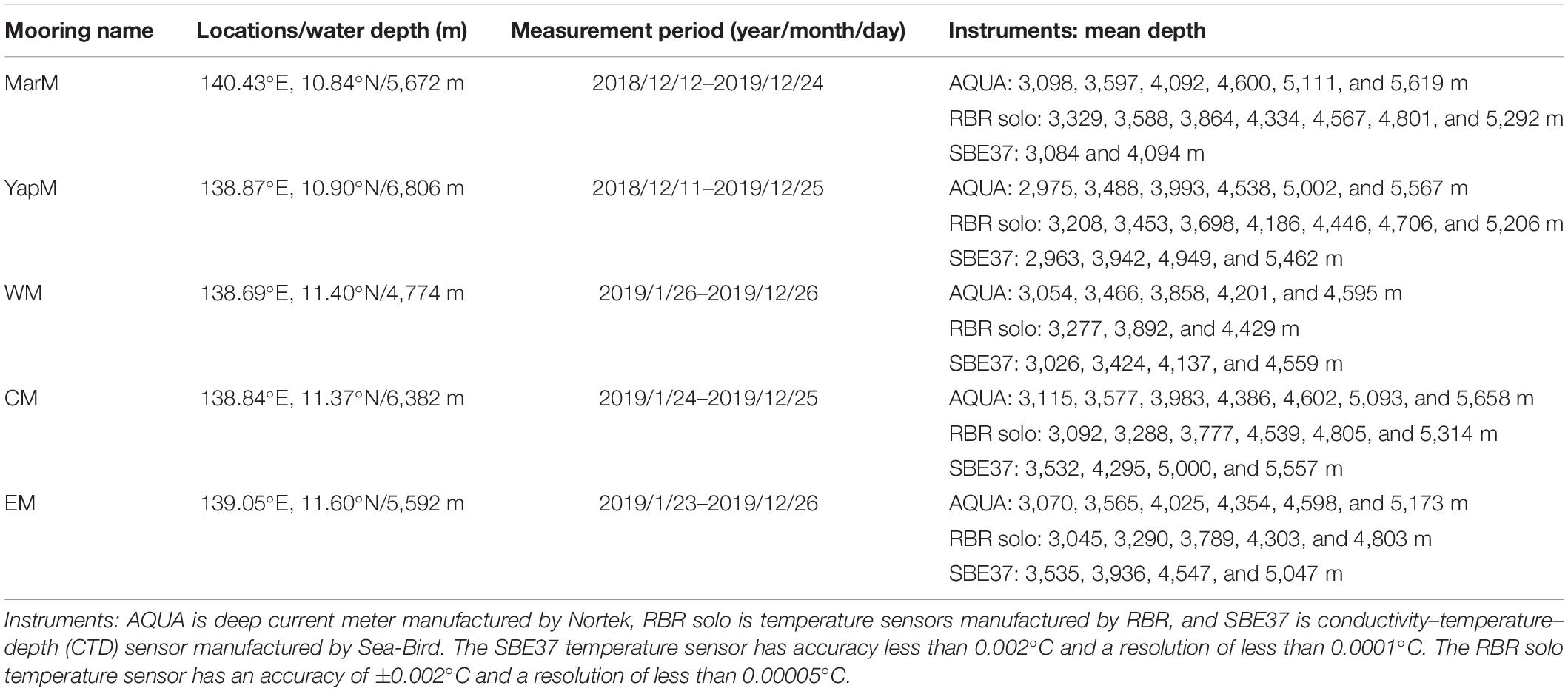
Table 1. The mooring locations and water depths, measurement periods, and instruments’ names and mean depths.

The MO Ocean Model Products

In order to gain insights into the variability of the L-PMOC at large spatiotemporal scales and to explore the underlying dynamics of the variations at the YMJ channels, we analyze two data assimilative global ocean modeling products created by Mercator Ocean (hereinafter MO), a contribution to the European Union Copernicus Marine Service¹. The two products are the analysis product PSY4V3R1 and the reanalysis product GLORYS12V1. From PSY4V3R1, we take daily fields of sea surface height (SSH), temperature, salinity, and velocity during our observation period. From GLORYS12V1, we take the monthly fields of the same variables over 1993–2018. Both products are created using the NEMO ocean model. The model has a horizontal resolution of 1/12° in longitude/latitude and 50 vertical levels with a resolution of 1 m at the surface and of 450 m near the bottom. The model uses the ETOPO1 bathymetry dataset in regions deeper than 300 m depth. The atmospheric fields from the ECMWF (European Centre for Medium-Range Weather Forecasts) Integrated Forecast System are used to force the ocean model. The altimeter measured SSH, in situ temperature, and salinity vertical profiles, and the satellite remote-sensing sea surface temperatures are jointly assimilated. For more details on the two products, readers are referred to Lellouche et al. (2013, 2018). The monthly wind stress datasets over 1993–2018 from the ECMWF ERA Interim are also analyzed to understand the variations of the SSH and water density from the MO models. The Ekman pumping velocity (EPV) is calculated as EPV = curl(τ/f)/ρ, where curl(τ) is the curl of wind stress, f is the Coriolis parameter, and ρ = 1,021 kg m^–3 is the mean water density within the Ekman layer.

Observed Variations of the L-PMOC

Observed Deep Flow and Potential Temperature

The observed along-channel velocities (U_along) at five mooring sites all exhibit seasonal cycles, and this variability suggests interconnections. Figure 2 presents the observed time-depth variations of potential temperature (θ) and U_along over depths greater than 3,000 m. Following previous studies (e.g., Johnson and Toole, 1993; Siedler et al., 2004; Wang et al., 2020), we take θ = 1.2°C as the boundary between the LCPW and UCPW, corresponding to the lower and upper deep layers, respectively. In the Eastern Channel, both the lower and upper deep layers show westward inflow into the YMJ with core speed reaching 30 cm s^–1 from the start of the measurement to the beginning of May 2019 and from November 2019 to the end of the measurement, and eastward outflow into the EMB or weak westward inflow from May to October 2019. In the Southern Channel, the core speed of the deep flow is reduced to 10 cm s^–1, and the flow southward into (northward out of) the WCB roughly corresponds to the deep inflow into (outflow out of) the YMJ in the Eastern Channel. We further calculate the lead–lag correlation of U_along at the MarM and YapM sites after applying a 31-day running mean to the observed time series (Figure 3A, same hereinafter). The correlation reaches peak values of 0.8–0.9 at the 95% confidence level with MarM leading YapM by 10–20 days at depths of 3,200–4,500 m, and with a nearly zero lag at depths greater than 4,500 m.

FIGURE 2

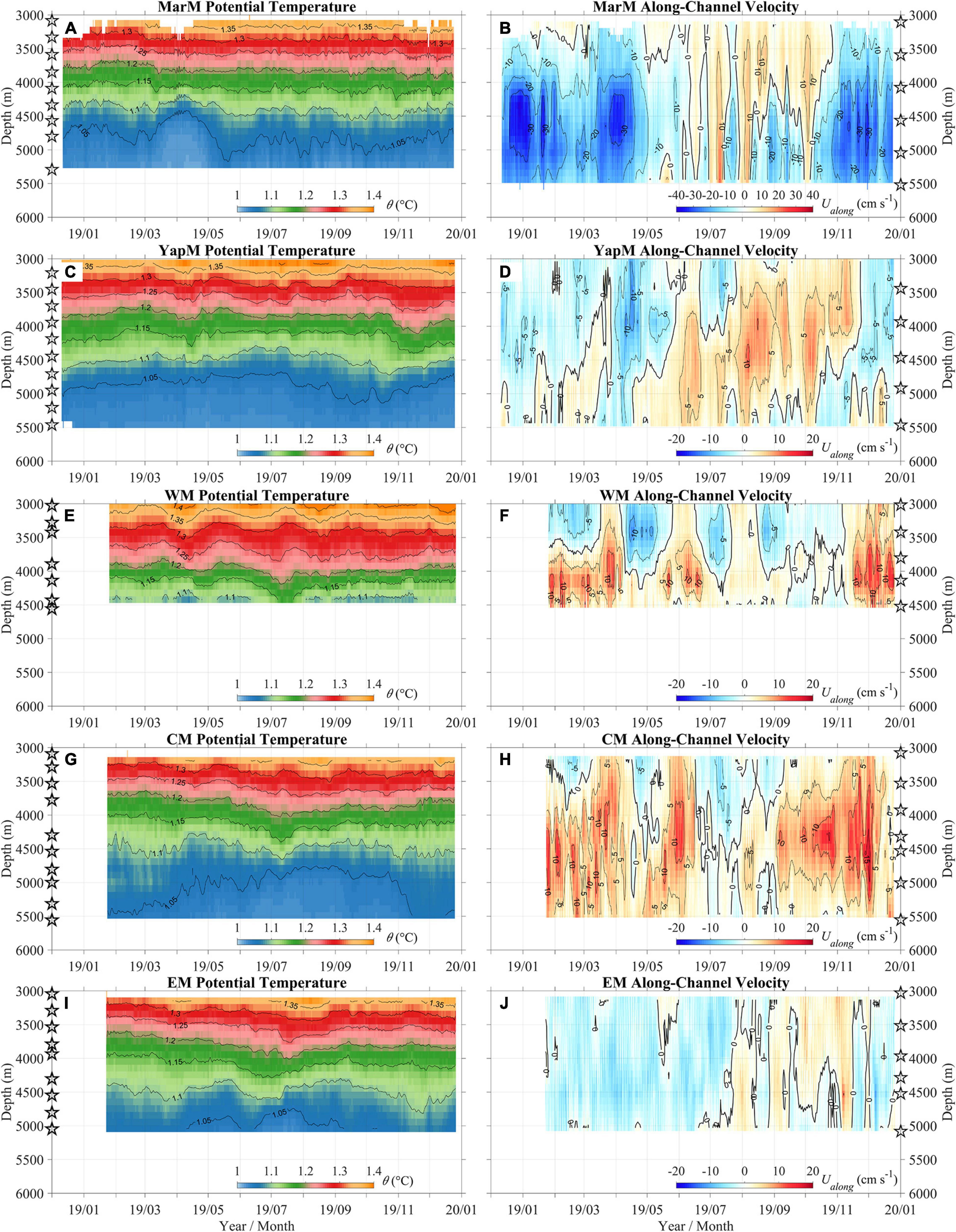
Figure 2. Time-depth variations of (left) potential temperature θ and (right) along-channel velocity U_along observed by moorings MarM (A,B), YapM (C,D), WM (E,F), CM (G,H), and EM (I,J). Open pentagrams indicate the depths of temperature sensors (left) and current meters (right).

FIGURE 3

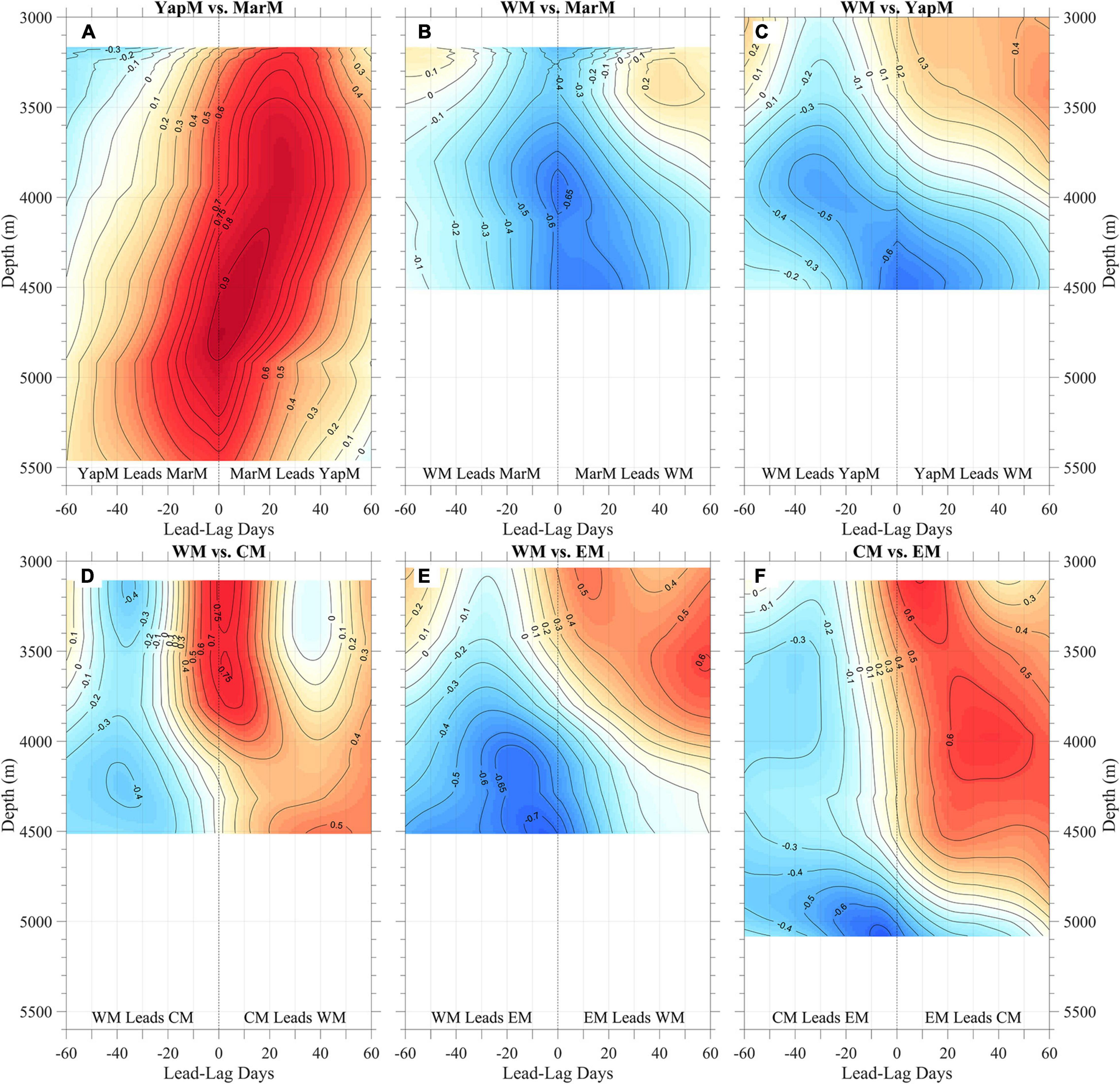
Figure 3. Lead–lag correlations of observed deep along-channel velocities between (A) YapM and MarM, (B) WM and MarM, (C) WM and YapM, (D) WM and CM, (E) WM and EM, and (F) CM and EM.

In the Northern Channel, the deep water at the WM site on average flows southward and northward in the upper and lower deep layers, respectively. In the lower deep layer, the relatively strong northward flow with a core speed of 10 cm s^–1 prevails from the start of the measurement to June 2019 and from mid-November 2019 to the end of the measurement, roughly corresponding to the westward inflow to the YMJ from the Eastern Channel. This is consistent with the fact that the WM U_along is inversely correlated with the MarM U_along with r = −0.6 to –0.65 at a zero lag (Figure 3B). A negative relationship with r = −0.6 at a zero lag also occurs between the WM and YapM U_along at depths greater than 4,000 m (Figure 3C). The seasonal cycle of U_along at the WM site is relatively weak in the upper deep layer and strong in the lower deep layer. The core speed of L-PMOC is 10 cm s^–1 in 2019, lower than the previously observed value of 20 cm s^–1 in 1997 and 15 cm s^–1 in 2017 at the WM site (Siedler et al., 2004; Wang et al., 2020). At the CM site, the northward flow is strong in both upper and lower deep layers with a core speed of 10 cm s^–1 during most of the measurement time and becomes weak or reverses during July–August 2019. The correlation between CM and WM U_along reaches 0.75 with CM leading WM by 2–10 days at 3,000–4,000 m and becomes weak at 4,000–4,500 m (Figure 3D). At the EM site, U_along is dominated by a weak southward flow in both layers. The correlation of deep flow at the EM site with that at the WM or CM site is positive in the upper deep layer with EM leading WM or CM by ∼10 days and is negative in the lower deep layer with WM or CM leading EM by 10–20 days (Figures 3E–F).

At the five mooring sites, variations of the deep flows are accompanied by changes in water mass properties (Figure 2). At the MarM site, the relatively low (high) θ roughly corresponds to the intensified inflow (outflow) to the YMJ in the lower deep layer, suggesting the influence of the L-PMOC intrusions. At the YapM site, the change of θ has no significant correlation with that of U_along and exhibits a weak seasonal variation. This may be due to the strong influence of the intraseasonal variability induced by energetic surface eddies and/or topographic Rossby waves (Ma et al., 2019; Wang et al., 2020). At the three mooring sites in the Northern Channel, the increase in the southward flow speed corresponds to a decrease in θ in the upper deep layer, implying the influx of the southward U-PMOC. In the lower deep layer with θ larger than 1.1°C, the decrease in θ corresponds to the increase in the northward flow speed at the WM and CM sites and in the southward flow speed at the EM site, suggesting the presence of the northward L-PMOC at the WM and CM sites and the presence of the southward return flow of the L-PMOC at the EM site (Wang et al., 2020). It should be noted that in the layer with θ lower than 1.1°C at the CM site, a positive relationship between θ and the northward L-PMOC intrusion flow speed suggests that there could be the remnants of previously intruded LCPW with older age. The intrusion and absence of the new LCPW causes the height of the remnant LCPW to fall and rise, respectively. The presence of the remnant LCPW only at the CM site is likely due to the greater depth at this site.

Estimated Volume Transports Based on Observations

We next estimate the volume transports in different potential temperature classes through each channel. For each channel, we grid the section with a resolution of 10 m in the horizontal and vertical directions. The data from the mooring measurements are extrapolated and interpolated into these grids. For each mooring, the observed U_along and θ are first interpolated vertically, and then the deepest measured value is extrapolated uniformly downward to the bottom. However, U_along in the last grid nearest the bottom is set to zero. The next step is horizontal extrapolation/interpretation. In the Eastern and Southern Channels, the observed U_along and θ are extrapolated uniformly to the bilateral grids at each depth, except for setting U_along to zero in the grids nearest the channel sidewalls. In the Northern Channel, the values of U_along and θ on mooring WM (EM) are extrapolated uniformly westward (eastward) to the western (eastern) sidewall, except for setting U_along to zero in the grids nearest the channel sidewalls. For the grids between WM and EM, the values of U_along and θ from moorings WM, CM, and EM at the same depth are linearly interpolated. The transect distributions of the MO modeled U_along and θ in the Eastern, Southern, Northern Channels (figure not shown) resemble those obtained from the above interpolation/extrapolation scheme. We then calculate the volume transports by integrating U_along from the isotherm depths of 1.15, 1.2, 1.25, and 1.3°C to the deepest layer and across the channel. We define the L-PMOC transport as all transport with θ less than 1.2°C.

The L-PMOC volume transports represented as mean ± standard deviation, are −2.43 ± 2.56 Sv (1 Sv = 10⁶ m³ s^–1) in the Eastern Channel and 0.42 ± 1.88 Sv in the Southern Channel during the 1-year cycle from December 15, 2018 to December 15, 2019, and 1.27 ± 1.23 Sv in the Northern Channel from January 26 to December 15, 2019 (Figures 4A–C). The L-PMOC transports in the three channels exhibit a prominent seasonal variation. An annual harmonic fit is applied to the time series of the estimated volume transports. Prior to the harmonic fit, each time series is smoothed with a 91-day running mean to focus on the variations longer than the intraseasonal time scales. We calculate R², defined as a ratio of the variance of the fitted time series to the variance of the smoothed observations. In the Eastern, Southern, and Northern Channels, the values of R² for the L-PMOC volume transports are 96, 91, and 85%, and the largest negative values of the fitted transport occur on January 26, February 8, and June 6, 2019, respectively. The variability of deep transports with θ less than 1.15, 1.25, and 1.3°C generally follow that with θ less than 1.2°C. The seasonal cycle of the L-PMOC transports in the three channels can be divided into two phases over November–April and May–October.

FIGURE 4

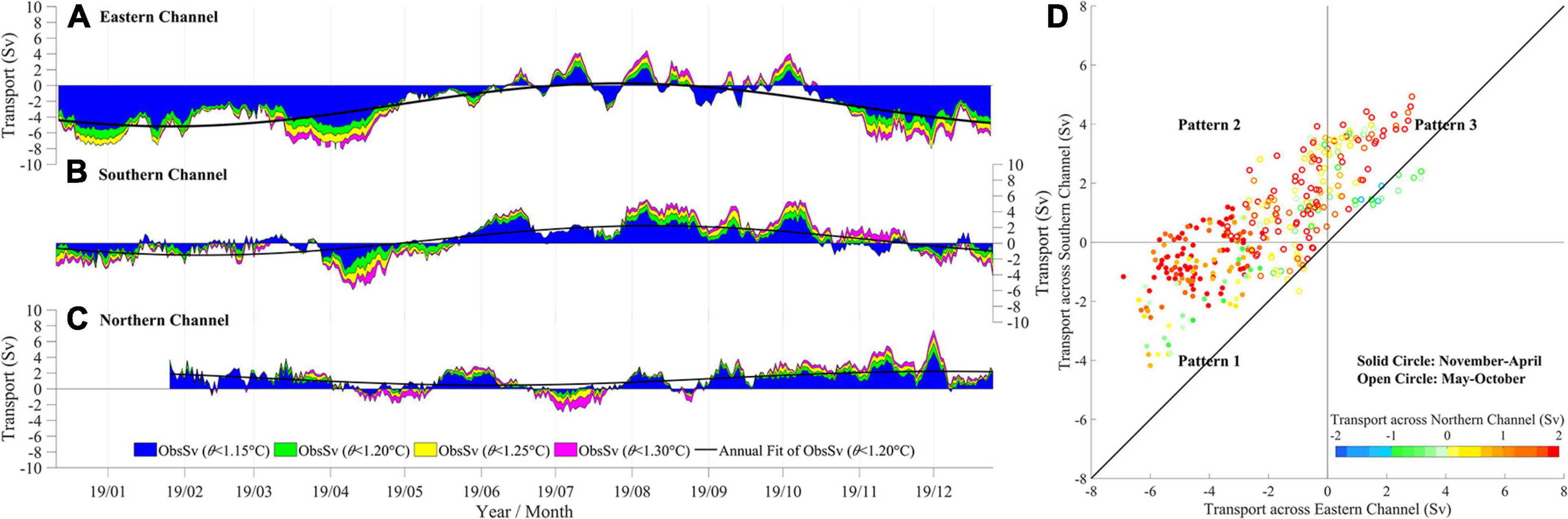
Figure 4. Stacked histograms of observed volume transport in potential temperature classes with θ less than 1.15°C (blue), 1.2°C (green), 1.25°C (yellow), and 1.30°C (pink) through the (A) Eastern, (B) Southern, and (C) Northern Channels. The annual harmonic fit of observed volume transports with θ less than 1.2°C is superimposed by black line in panels (A–C). (D) Scatter diagram of volume transports with θ less than 1.2°C through the Eastern Channel versus through the Southern Channel, with a thick line depicting the 1:1 ratio. The color shading denotes the volume transports with θ less than 1.2°C through the Northern Channel. Solid and open circles represent the values obtained during November–April and May–October, respectively.

In order to explore the L-PMOC pathways at the YMJ, we plot the scatter diagram of the observed volume transports, with the x-axis, y-axis, and color shading denoting the transports in the Eastern, Southern, and Northern Channels, respectively (Figure 4D). The L-PMOC pathways can be mainly cataloged into three patterns based on the scatter diagram. In Pattern 1, the L-PMOC flows westward into the YMJ through the Eastern Channel and then bifurcates into the southern and northern branches. The southern branch passes through the Yap Trench and finally flows into the WCB, while the northern branch flows mainly through the Northern Channel into the WMB. In Pattern 2, the lower deep water flow comes partly from the WCB, directed northward through the Southern Channel, and partly from the EMB, directed westward through the Eastern Channel. Then the combined transport passes through the Northern Channel into the WMB. In Pattern 3, the lower deep water flow originates in the WCB and moves northward through the Southern Channel. A portion of this northward flow turns eastward and flows out of the YMJ region through the Eastern Channel. The deep flow through the Northern Channel is mainly northward and occasionally southward. In Patterns 2 and 3, the northward flow in the Southern Channel coming from the WCB can be regarded as the return flow of the L-PMOC. The flow pattern with eastward transport through the Eastern Channel and southward transport through the Southern Channel does not occur, suggesting that the lower deep transport cannot solely originate from the WMB. Pattern 1 mainly occurs during the seasonal phase from November to April, and Patterns 2 and 3 mainly occur during the seasonal phase from May to October. During November–April (May–October), the mean and standard deviation of the L-PMOC transports are −4.44 ± 1.26 (−0.30 ± 1.47), −0.96 ± 1.13 (1.75 ± 1.49), and 1.49 ± 1.31 (1.07 ± 1.10) Sv in the Eastern, Southern, and Northern Channels (right panels of Figure 1). The transports through three channels are imbalanced, especially during November–April. The possible reasons include uncertainty in the transport estimate, and the unknown transport through the deep channel east of the Southern Channel. During November–April, a part of deep water may flow southward into WCB through this channel.

Simulated Variations of the L-PMOC

From the pointwise mooring measurements of deep velocity and temperature, it is difficult to depict the deep flow across the large spatial scale at the YMJ. The observations covered only 1 year; hence, the robustness on the seasonal signal needs to be assessed with long time series of reliable ocean model simulations. Here, we resort to the high-resolution data-assimilated MO results. Figure 5 shows the time-depth variations of the MO modeled U_along and θ at five locations, each in the horizontal model grid that is nearest to the site of one of the five moorings. The comparison of the model results with observations is assessed with the correlation coefficients and the normalized root-mean-square deviation ($\text{NRMSE}=\sqrt{\frac{1}{\text{n}}{\sum }_1^{\text{n}}{(\text{Obs}-\text{MO})}^2}/(\max (\text{Obs})-\min (\text{MO}))$, where n is the number of data values), calculated for the daily time series of U_along and θ from observations (Obs) and the MO outputs (MO), after applying a 5-day running mean. At the YapM, MarM, and WM sites, the correlations are larger than 0.55 and NRMSEs are less than 35%. The agreements are poor at the CM and EM sites, mainly due to the failure of MO in reproducing the U-PMOC and the return flow of the L-PMOC, consistent with the previous evaluation in Wang et al. (2020).

FIGURE 5

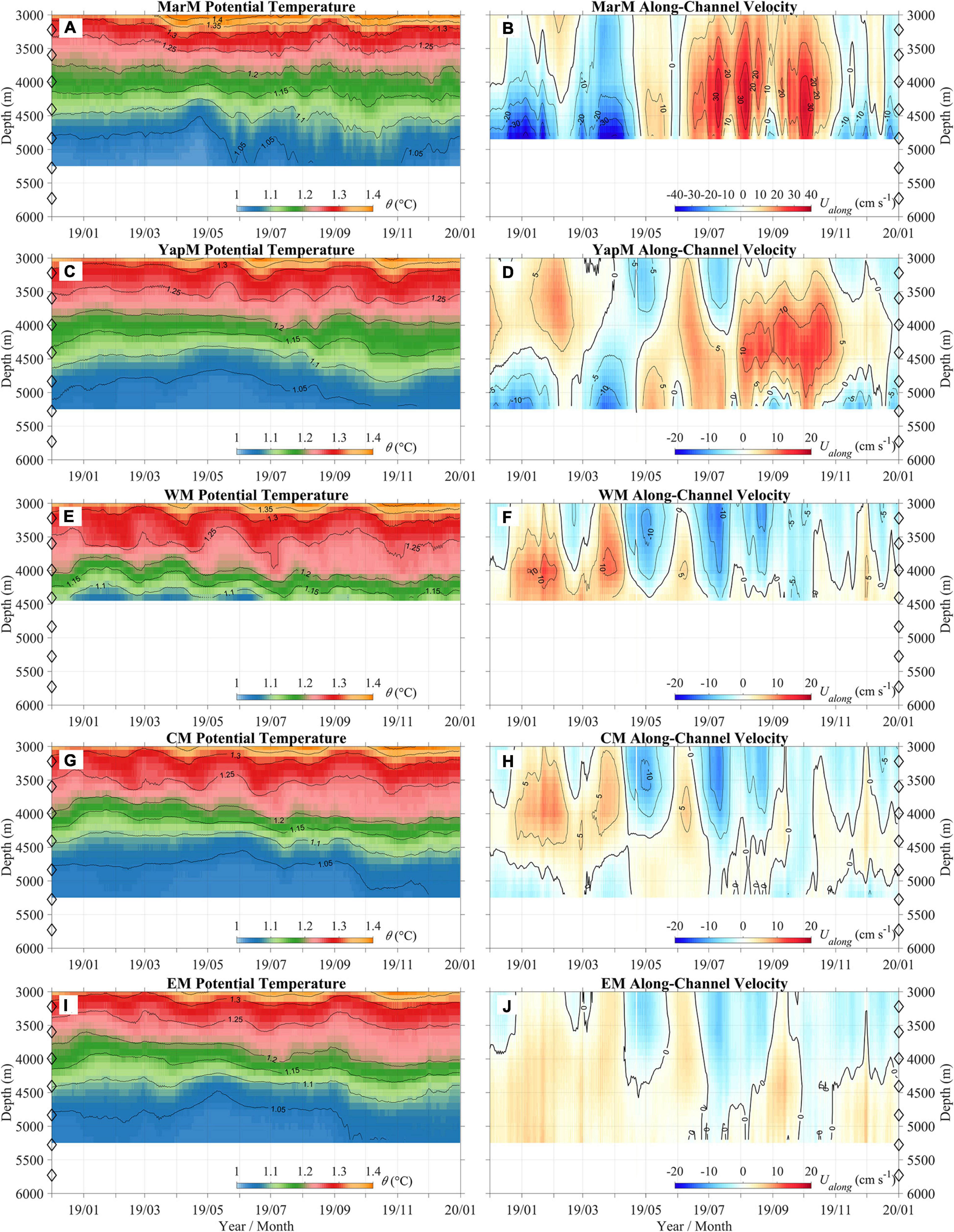
Figure 5. Time-depth variations of MO modeled (left) potential temperature θ and (right) along-channel velocity U_along at the mooring sites of MarM (A,B), YapM (C,D), WM (E,F), CM (G,H), and EM (I,J). Open diamonds indicate the depths of model vertical levels.

We further calculate the modeled volume transport in the three channels (Figures 6A–C). There are four, five, and six simulated profiles in the transects of Eastern, Southern, and Northern Channels, respectively. We filled the missing data using the same interpolation/extrapolation scheme as used for the observations in the Northern Channel. During November–April (May–October) over the mooring measurement period, the mean and standard deviation of the modeled L-PMOC transports are −2.18 ± 1.69 (2.49 ± 1.44), −0.33 ± 1.47 (3.43 ± 1.33), and 1.20 ± 1.00 (0.37 ± 1.02) Sv in the Eastern, Southern, and Northern Channels. In the same order of the three channels calculated for the 5-day running mean L-PMOC transports from observation and model outputs, the correlations are 0.93, 0.77, and 0.37, and the NRMSEs are 29, 22, and 23%, respectively. During the same period as observations, the modeled L-PMOC transport also exhibits an evident seasonal cycle with R² reaching 93, 79, and 70%. In the Eastern Channel, the MO model reproduces well the seasonal variability but has biases in the magnitude, with smaller westward transport during November–April and larger eastward transport during May–October. In the Southern Channel, the MO model performs well in both the seasonal cycle and magnitude. In the Northern Channel, the MO model performs well during most of the measurement period but fails in reproducing the northward transport from mid-September to mid-November, leading to a low correlation. Despite these discrepancies, the similarity between the MO model and the observations in terms of the seasonal variation of the L-PMOC encourages further examination of the MO results to identify the seasonal variation of the L-PMOC over the whole YMJ region and over a longer time scale, and to explore the underlying mechanism.

FIGURE 6

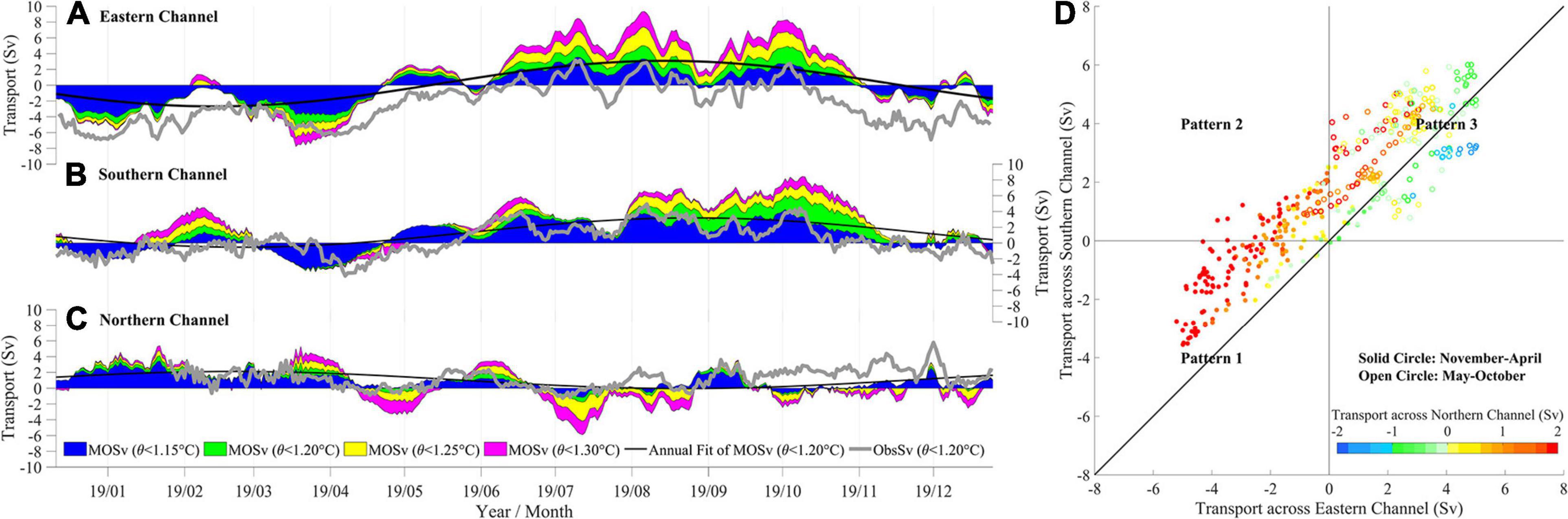
Figure 6. Stacked histograms of MO modeled volume transport in potential temperature classes with θ less than 1.15°C (blue), 1.2°C (green), 1.25°C (yellow), and 1.30°C (pink) through the (A) Eastern, (B) Southern, and (C) Northern Channels. The annual harmonic of modeled volume transports with θ less than 1.2°C is superimposed by black line in panels A–C. The thick grey lines in panels A–C denote the observed volume transports with θ less than 1.2°C in three corresponding channels. (D) Scatter diagram of modeled volume transports with θ less than 1.2°C through the Eastern Channel versus through the Southern Channel, with a thick line depicting the 1:1 ratio. The color shading denotes the modeled volume transports with θ less than 1.2°C through the Northern Channel. Solid and open circles represent the values obtained during November–April and May–October, respectively.

Based on the MO daily transports during the mooring measurement period, we also plot a scatter diagram of the volume transports in three channels (Figure 6D). The results show three patterns similar to those obtained from the observations. However, the principal occurrence time of Pattern 2 is shifted to November–April. The flow patterns of the L-PMOC at the YMJ are depicted by the horizontal distributions of the depth-integrated MO velocity with θ less than 1.2°C during the three patterns (Figure 7). The flow pathways are generally in accordance with that inferred from observations.

FIGURE 7

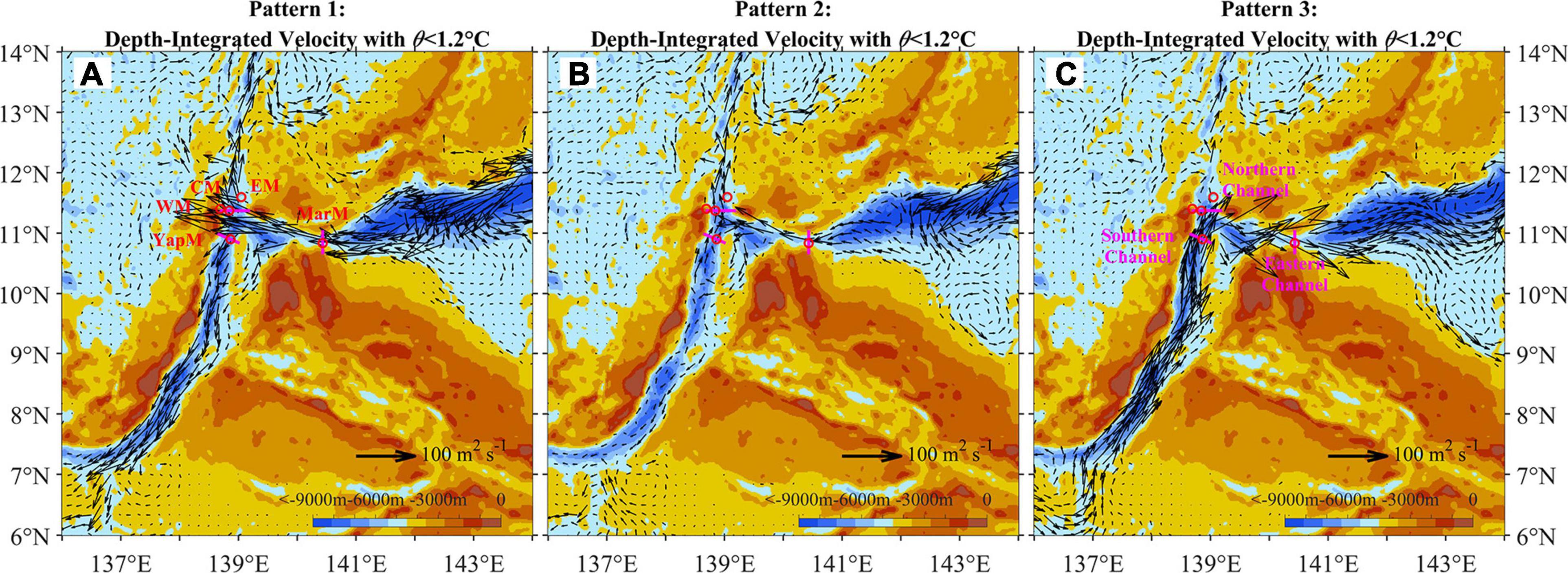
Figure 7. Horizontal distributions of depth-integrated MO velocity with potential temperature θ < 1.2°C (arrows) averaged over Patterns (A) 1, (B) 2, and (C) 3 at the Yap-Mariana Junction. Patterns 1, 2, and 3 are defined in Figure 6. Locations of five subsurface moorings are denoted by red open circles. The cross sections of Eastern, Southern, and Northern Channels are indicated by pink lines. The bathymetry is from ETOPO1.

The seasonal variability of the L-PMOC volume transports in the three channels is evident in the longer time series of the MO outputs over 1993–2018 (Figure 8). The “climatological” seasonal signals are obtained by applying the annual harmonic fit to each volume transport time series, and the fitted annual cycle explains 93, 94, and 80% of the total variance in the Eastern, Southern, and Northern Channels, respectively. This provides further evidence of the seasonal variability of the L-PMOC at the YMJ. The volume transports in the three channels over 1993–2018 also show variations at the interannual and longer time scales. During November–April, a decreasing trend appears in the L-PMOC transports from the EMB to the YMJ through the Eastern Channel and then from the YMJ to the WMB and WCB through the Northern and Southern Channels. In contrast, during May–October, an increasing trend appears in the L-PMOC transports from the WCB and WMB to the YMJ through the Southern and Northern Channels and then from the YMJ to the EMB through the Eastern Channel. However, such interannual variability cannot be verified with the limited observation and is not discussed further here.

FIGURE 8

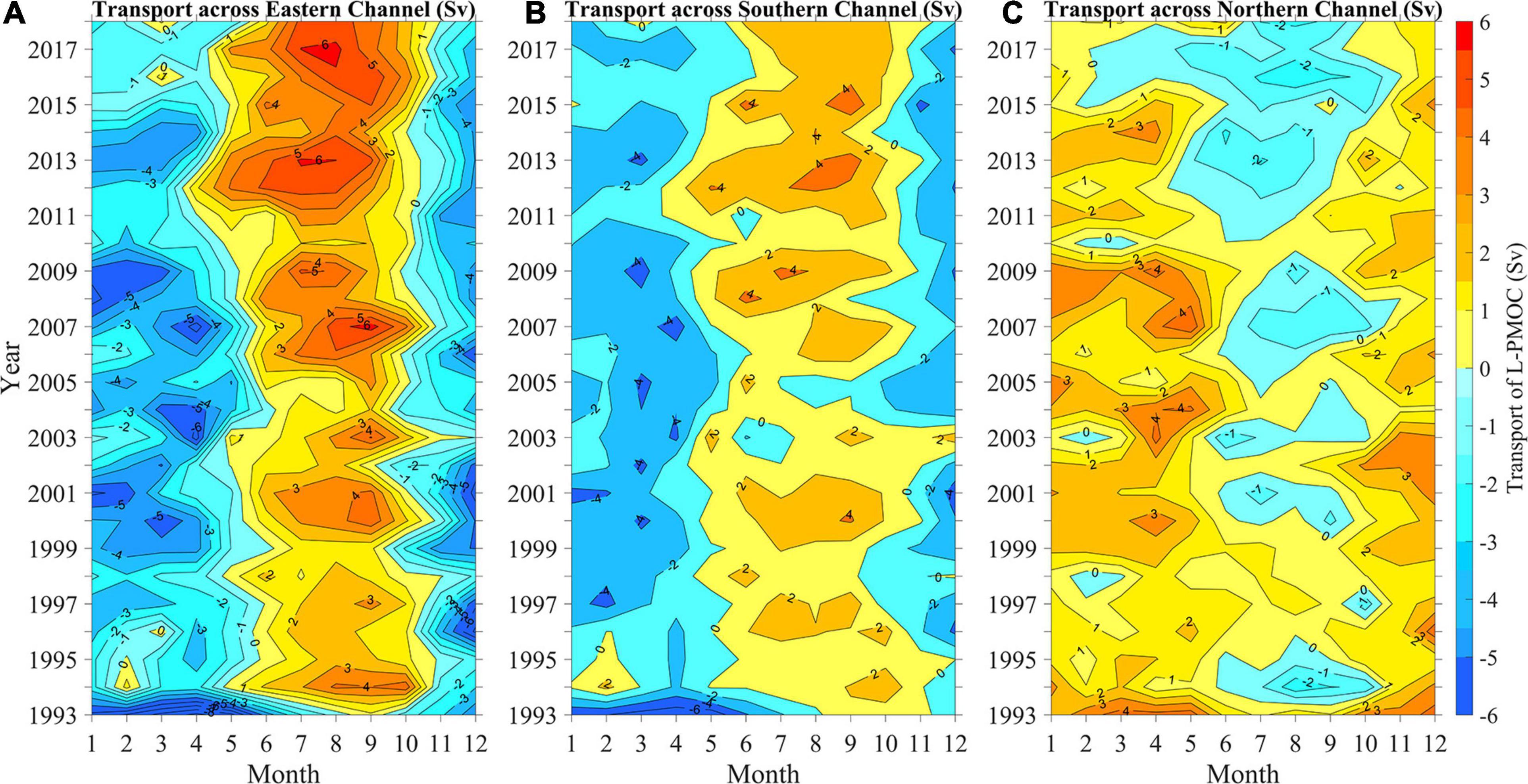
Figure 8. MO monthly volume transports of the L-PMOC through the (A) Eastern, (B) Southern, and (C) Northern Channels from 1993 to 2018.

Forcing Mechanisms of the L-PMOC

The forcing mechanisms for the pathways and seasonal variability of the L-PMOC are explored through analysis of the MO model solutions. Deep-water exchange between two interconnected basins can be forced by the gradient of deep pressure along the channels (Sprintall et al., 2013). We select two representative sites on the northeastern and southwestern sides of the YMJ region (hereafter referred to as NE and SW, NE site: 140.83°E/10.83°N, SW site: 136.9°E/6.83°N, Figure 9A) and examine their pressure difference. At each point, the pressure P at the depth z is calculated using the hydrostatic equation P=∫^zgdz (where ρ is water density, g is gravitational acceleration, and η is SSH) based on the MO monthly data over 1993–2018. The correlations of monthly time series of the pressure difference between NE and SW (P_Diff = P_NE – P_SW) at 4,405 m with those of the modeled L-PMOC transports across the Eastern and Southern Channels reach −0.95 and −0.86, respectively. At depths greater than 2,000 m, the climatological monthly P_Diff is positive from November to April, corresponding well to the modeled L-PMOC transport from the EMB to the WCB, and is negative from May to October, corresponding well to the modeled return flow of L-PMOC from the WCB to the EMB (Figures 8 and 9B). Additional trials suggest that these results are not sensitive to the specific locations of two points in two adjacent basins.

FIGURE 9

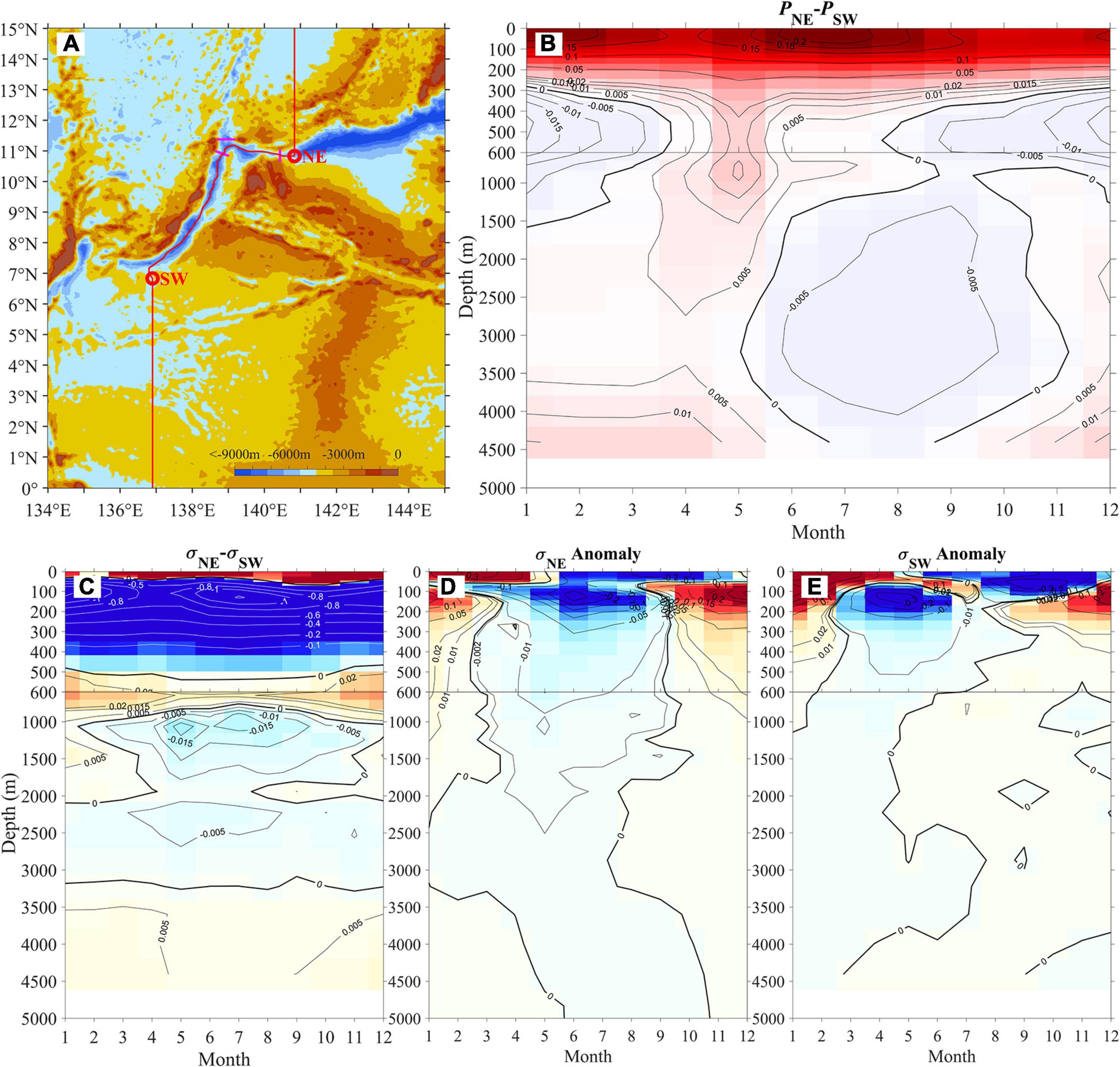
Figure 9. (A) Map of topography near the Yap-Mariana Junction (YMJ) showing two representative sites (red circles) in the northeastern (NE) and southwestern (SW) sides of the YMJ channels and meridional section (red curve). Vertical distributions of climatological monthly (B) pressure and (C) potential density difference between the NE and SW sites, and potential density anomalies at the (D) NE and (E) SW sites.

At each depth, P_Diff is determined by SSH difference (SSH_diff = SSH_NE – SSH_SW) and the vertically integrated water density difference (D_Diff = D_NE – D_SW) from the surface to that depth. From the vertical distributions of climatological monthly P_Diff and D_Diff (Figures 9B,C), we can distinguish four key layers that play a decisive role in determining the mean value and variability of P_Diff in the lower deep layer. The four layers roughly correspond to the depth ranges over the upper 50 m with mean positive D_Diff, 50–500 m with mean negative D_Diff, 500–850 m with mean positive D_Diff, and 850–2,000 m with seasonal positive and negative D_Diff. At depths greater than 2,000 m, the value of D_Diff is very small, corresponding to the negligible change of P_Diff with depth.

The mean values of D_Diff in the above four layers are mainly related to the differences in water mass properties (Figure 10). In the surface mixed layer roughly over 0–50 m depth, the positive D_Diff can be related to the larger salinity at the NE than at the SW sites, which is caused by the difference in the air–sea water exchange (precipitation minus evaporation) between the two sites. The mean negative D_Diff at 50–500 m is mainly controlled by the potential temperature difference over the 22.5–25.5-σ_θ sublayer and by the salinity difference over the 25.5–27.0-σ_θ sublayer, respectively. In the upper sublayer, the potential temperature of the North Pacific Tropical Water (NPTW) at the NE site is higher than that of the North Pacific tropical subsurface water (TSSW, Wang et al., 2013) at the SW site. In the lower sublayer, the water mass at the SW site is the mixture of TSSW and Antarctic Intermediate Water (AAIW, Qu and Lindstrom, 2004), the salinity of which is higher than that of the North Pacific Intermediate Water (NPIW) at the NE site. The mean positive SSH_diff can be primarily related to the “steric” effects of D_Diff at 50–500 m.

FIGURE 10

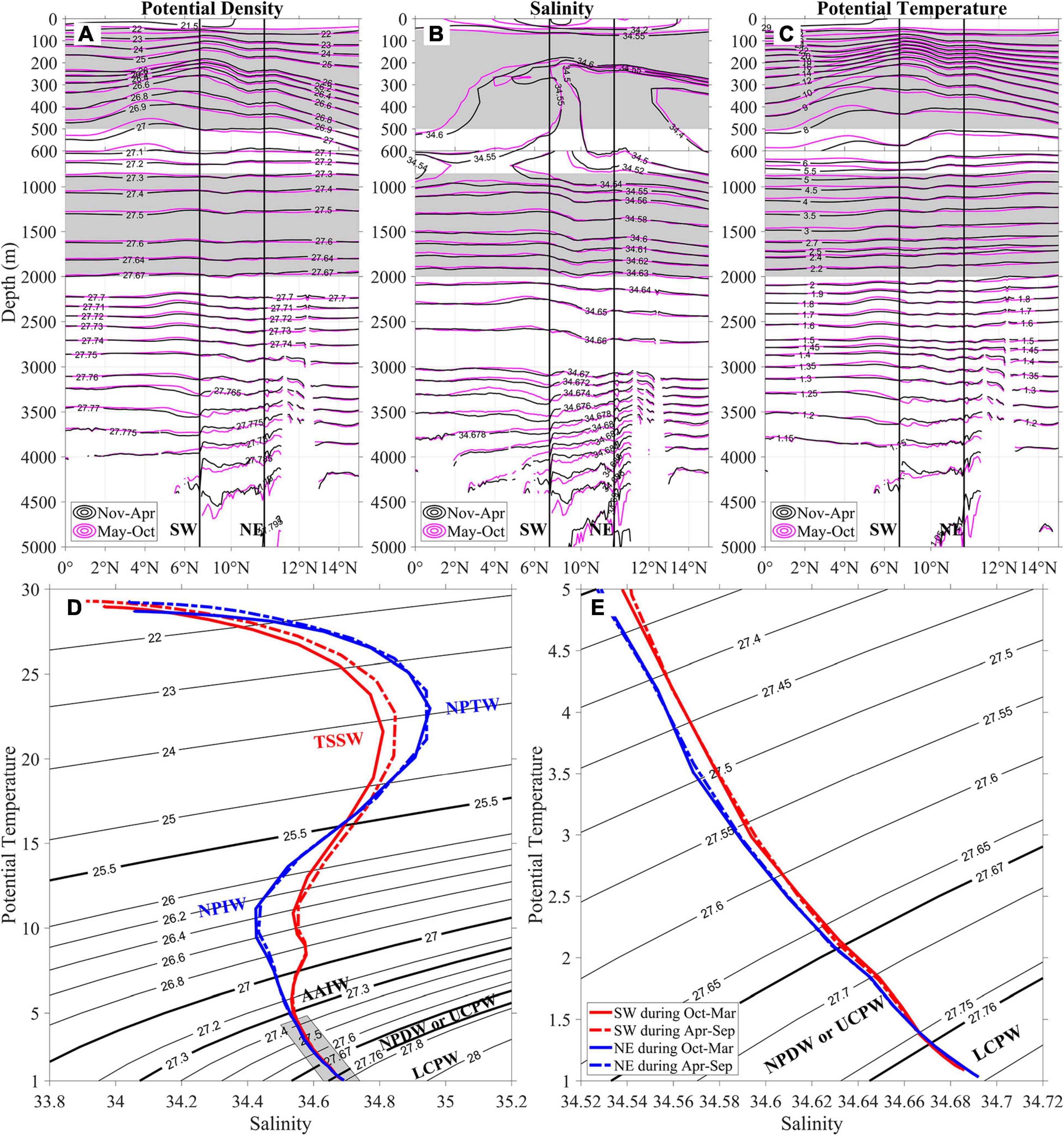
Figure 10. Vertical distributions of mean (A) potential density, (B) salinity, and (C) potential temperature along the section denoted by red curve in Figure 9A during November–April (black contours) and May–October (pink contours). Gray shadings are superimposed to help separate four key layers for determining the pressure difference between NE and SW (see text). (D) Relationships between potential temperature and salinity at the SW and NE sites with (E) a zoomed-in view on the isopycnals below 27.35 kg m^–3.

In the two following layers, both sites are occupied by the AAIW at 500–850 m, and the mixture of the AAIW and the UCPW or the North Pacific Deep Water (NPDW) at 850–2,000 m. The UCPW occupies almost the same depth range as the NPDW. Compared to the NPDW, the UCPW is characterized by slightly higher salinity; however, the two water masses are difficult to identify locally (Kawabe and Fujio, 2010). The mean salinity and potential temperature in the two layers decrease northward (Figure 10). At 500–850 m, the mean positive D_Diff is related to the lower potential temperature at the NE than at the SW sites. At 850–2,000 m, the potential density is controlled by the potential temperature (salinity) over November–April (May–October), leading to the positive (negative) D_Diff.

Next, we explore the causes of seasonal variations of SSHs (Figures 11C,D) and water densities (Figures 9D–E) at the NE and SW sites. The seasonality of SSH_diff and D_Diff can be caused by both local Ekman pumping and the westward-propagating Rossby waves that are remotely forced (e.g., Vivier et al., 1999; Zhao et al., 2012). At the NE site, the SSHs during October–March and April–September are related to the westward propagation of negative and positive signals, respectively (Figure 11C). Their phase speeds approximately equal to 1.48 m s^–1, much higher than the typical phase speed of the 1st baroclinic mode Rossby wave along the NE’s latitude (0.4 m s^–1, Kessler, 1990). This suggests that the signals are influenced by both the westward-propagating Rossby wave generated by EPVs in the eastern Pacific and the local Ekman pumping (Figures 11A,C). For the water density at the NE site, the forcing mechanism for its seasonal variability at depths shallower than 380 m is similar to that for the SSH (Figures 11E,G). At depths greater than 380 m, the local Ekman pumping effect vanishes, and the seasonal variability is mainly related to the Rossby waves generated by EPVs near 160°E (Figure 11I). The phase speed is estimated to be 0.2 m s^–1, very close to the typical speed of the 2nd baroclinic mode Rossby wave along the NE’s latitude (0.16 m s^–1). At depths greater than 2,225 m, the 2nd baroclinic mode Rossby wave can also be seen in the central and eastern Pacific but is not visible in the western part due to the blocking of topography (figure not shown).

FIGURE 11

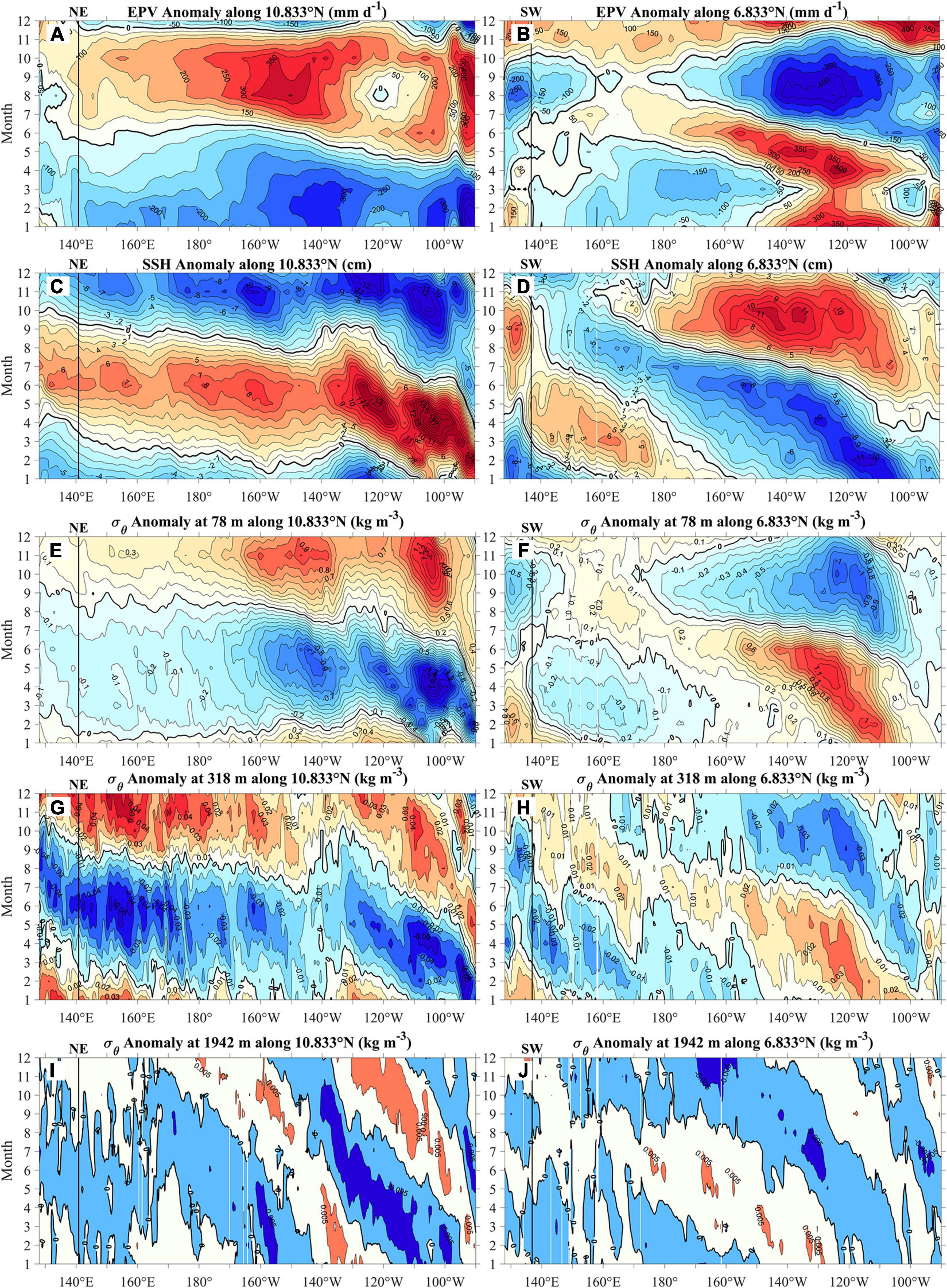
Figure 11. Longitude-time variations of anomalies of (A,B) Ekman pumping velocity – EPV, (C,D) sea surface height – SSH, and potential density σ_θ at (E,F) 78 m, (G,H) 318 m, (I,J) 1942 m along the latitudes (10.833°N and 6.833°N) of (left) NE and (right) SW sites. Black lines denote the locations of NE and SW sites.

At the SW site, the negative and positive SSHs during November–February and July–October are produced by local negative and positive EPVs, respectively, while SSHs during March–June are related to the westward propagation of downwelling Rossby waves triggered by negative EPV near the dateline (Figures 11B,D). The phase speed of the waves is 0.5 m s^–1, very close to the typical speed of the 2nd baroclinic mode Rossby waves along the SW’s latitude (0.52 m s^–1). For the water density at the SW site, seasonal variability at depths less than 318 m is influenced primarily by the local EPVs and secondarily by the Rossby waves, resembling the behavior of SSHs (Figure 11F). At depths of 318–644 m, the influence from the local Ekman pumping is still present, but the Rossby waves are generated by the EPV near 150°E (Figure 11H). The westward-propagating wave speed is 0.10 m s^–1, very close to the typical phase speed of the 3rd baroclinic mode Rossby waves along the SW’s latitude (0.13 m s^–1). At depths greater than 644 m, the contribution from the local Ekman pumping vanishes, and the 3rd baroclinic mode Rossby waves play a dominant role in the seasonal variability (Figure 11J). At depths greater than 3,221 m, the 3rd baroclinic mode Rossby waves can also be seen in the central and eastern Pacific but are not visible in the western part due to the topographic blocking (figure not shown).

In summary, the L-PMOC transport at the YMJ corresponds to the local pressure gradient between two interconnected basins in the lower deep layer. The differences in SSH and water density at depths less than 2,000 m between the NE and SW sites play a decisive role in forming the lower deep pressure gradient. In contrast, the water density difference at depths greater than 2,000 m plays a minor role. The local Ekman pumping and westward-propagating Rossby waves are combined to determine the seasonal variability of SSH and water density in the upper 2,000-m layer, and consequently the L-PMOC volume transport. That is to say, the L-PMOC transport greater than 3,500 m is closely linked to the wind forcing and the upper ocean processes at depths less than 2,000 m.

Conclusion

At the Pacific YMJ, a major gateway for L-PMOC flowing into the WPO, five subsurface moorings were deployed in three deep channels to reveal the pathways, volume transport, and seasonal variability of L-PMOC. The pathways of L-PMOC at the YMJ can be cataloged into three patterns. In the first pattern, the L-PMOC flows westward into the YMJ through the Eastern Channel, and then bifurcates into a southern branch, directed towards the WCB, and a northern branch, directed towards the WMB. In the second pattern, the lower deep water flows into the YMJ through the Eastern and Southern Channels, and then flows northward into the WMB. In the third pattern, a northward return flow of L-PMOC through the Southern Channel bifurcates into an eastward branch towards the EMB and a northward branch towards the WMB. The volume transport of L-PMOC through the Eastern, Southern, and Northern Channels exhibits seasonality. The L-PMOC pathway during November–April is consistent with Pattern 1, and that during May–October conforms to Patterns 2 and 3. The L-PMOC volume transports with θ less than 1.2°C, represented as mean ± standard deviations, are −4.44 ± 1.26 (−0.30 ± 1.47), −0.96 ± 1.13 (1.75 ± 1.49), and 1.49 ± 1.31 (1.07 ± 1.10) Sv in Eastern, Southern, and Northern Channels during November–April (May–October).

Large spatiotemporal fields of the MO model outputs were analyzed to explore the driving mechanism for the L-PMOC pathways and seasonality at the YMJ. The MO outputs generally perform well in simulating the seasonal variation of L-PMOC transports at the YMJ. The modeled flow pathways resemble that inferred from the observation. Long time series of MO monthly L-PMOC transports in three channels during 1993–2018 also exhibit evident seasonal variability. The L-PMOC transports at the YMJ are driven by local pressure gradients between two adjacent basins in the lower deep layer, mainly set up by differences in the SSH and water mass density in the upper 2,000-m layer. The local Ekman pumping and westward-propagating Rossby wave triggered by remote Ekman pumping are largely responsible for the seasonal variability of L-PMOC.

Most importantly, the relationship of the L-PMOC transport greater than 3,500 m at the YMJ with wind forcing and water mass properties over the upper 2,000 depths are established. This relationship can partially explain why the MO model has a good performance in simulating the L-PMOC. The reanalysis dataset usually has a good capability in reproducing the upper ocean processes due to the assimilation of observed wind, SSH, and in situ temperature and salinity vertical profiles in the upper 2,000-m layer. Additional analysis of the HYCOM GOFS 3.0 outputs suggests that the HYCOM model can also reproduce the volume transport and seasonal variability of L-PMOC quite well (figure not shown). Whether such a relationship can be applied to the L-PMOC transports in the upstream and downstream regions deserves further investigation. Filling in our descriptive picture and theoretical understanding of the L-PMOC system, and its variability on scales from seasonal to decades, remains a daunting challenge. It is hoped that our study will stimulate more in situ measurements in other locations along the L-PMOC route and more analyses and further improvements of the ocean models to quantify and understand the L-PMOC variability and forcing mechanisms.

Data Availability Statement

The raw data supporting the conclusions of this article will be made available by the authors, without undue reservation.

Author Contributions

JW and FW initiated the idea and designed the observation. JW analyzed the data and wrote the manuscript. FW, YL, QM, LP, and ZZ contributed to the refinements of the data analysis and manuscript writing. All authors contributed to the article and approved the submitted version.

Funding

This study was supported by the Strategic Priority Research Program of the Chinese Academy of Sciences (grant XDA22000000), the National Natural Science Foundation of China (grants 91958204 and 41776022), the Key Research Program of Frontier Sciences, CAS (grant QYZDB-SSW-SYS034), and the International Partnership Program of CAS (grant 133137KYSB20180056). FW thanks the support from the National Natural Science Foundation of China (grants 41730534 and 41421005). QM thanks the support by the National Natural Science Foundation of China (grant 42006003).

Conflict of Interest

The authors declare that the research was conducted in the absence of any commercial or financial relationships that could be construed as a potential conflict of interest.

The reviewer YS declared a past co-authorship with one of the authors, FW, to the handling editor.

Footnotes

1. ^ https://resources.marine.copernicus.eu/

References

Callahan, J. E. (1972). The structure and circulation of deep water in the Antarctic. Deep Sea Res. Oceanogr. Abstr. 19, 563–575. doi: 10.1016/0011-7471(72)90040-x

CrossRef Full Text | Google Scholar

Johnson, G. C., Mecking, S., Sloyan, B. M., and Wijffels, S. E. (2007). Recent bottom water warming in the Pacific Ocean. J. Climate 20, 537165–5375. doi: 10.1175/2007JCLI1879.1

CrossRef Full Text | Google Scholar

Johnson, G. C., and Toole, J. M. (1993). Flow of deep and bottom waters in the Pacific at 10°N. Deep Sea Res. I 40, 371–394. doi: 10.1016/0967-0637(93)90009-R

CrossRef Full Text | Google Scholar

Kawabe, M., and Fujio, S. (2010). Pacific Ocean circulation based on observation. J. Oceanogr. 66, 389–403. doi: 10.1007/s10872-010-0034-8

CrossRef Full Text | Google Scholar

Kawabe, M., Fujio, S., and Yanagimoto, D. (2003). Deep-water circulation at low latitudes in the western North Pacific. Deep Sea Res. 50, 631–656. doi: 10.1016/S0967-0637(03)00040-2

CrossRef Full Text | Google Scholar

Kawabe, M., Fujio, S., Yanagimoto, D., and Tanaka, K. (2009). Water masses and currents of deep circulation southwest of the Shatsky Rise in the western North Pacific. Deep Sea Res. I 56, 1675–1687. doi: 10.1016/j.dsr.2009.06.003

CrossRef Full Text | Google Scholar

Kawabe, M., Yanagimoto, D., and Kitagawa, S. (2006). Variations of deep western boundary currents in the Melanesian Basin in the western North Pacific. Deep Sea Res. I 53, 942–959. doi: 10.1016/j.dsr.2006.03.003

CrossRef Full Text | Google Scholar

Kessler, W. S. (1990). Observations of long rossby waves in the northern tropical pacific. J. Geophys. Res. Oceans 95, 5183–5217. doi: 10.1029/jc095ic04p05183

CrossRef Full Text | Google Scholar

Lellouche, J. M., Greiner, E., Galloudec, O. L., Garric, G., Regnier, C., Drevillon, M., et al. (2018). Recent updates to the copernicus marine service global ocean monitoring and forecasting real-time 1/12° high-resolution system. Ocean Sci. 14, 1093–1126. doi: 10.5194/os-14-1093-2018

CrossRef Full Text | Google Scholar

Lellouche, J. M., Le Galloudec, O., Drévillon, M., Régnier, C., Greiner, E., Garric, G., et al. (2013). Evaluation of global monitoring and forecasting systems at Mercator Ocean. Ocean Sci. 9:57. doi: 10.5194/os-9-57-2013

CrossRef Full Text | Google Scholar

Ma, Q., Wang, F., Wang, J., and Lyu, Y. (2019). Intensified deep ocean variability induced by topographic rossby waves at the pacific yap−mariana junction. J. Geophys. Res. Oceans 124, 8360–8374. doi: 10.1029/2019JC015490

CrossRef Full Text | Google Scholar

Mantyla, A. W., and Reid, J. L. (1983). Abyssal characteristics of the World Ocean waters. Deep Sea Res. Part A Oceanogr. Res. Pap. 30, 805–833. doi: 10.1016/0198-0149(83)90002-x

CrossRef Full Text | Google Scholar

Pratt, L. J., Voet, G., Pacini, A., Tan, S., Alford, M. H., Carter, G. S., et al. (2019). Pacific abyssal transport and mixing: through the Samoan Passage versus around the Manihiki Plateau. J. Phys. Oceanogr. 49, 1577–1592. doi: 10.1175/JPO-D-18-0124.1

CrossRef Full Text | Google Scholar

Qu, T., and Lindstrom, E. J. (2004). Northward intrusion of antarctic intermediate water in the western Pacific. J. Phys. Oceanogr. 34, 2104–2118. doi: 10.1175/1520-0485(2004)034<2104:nioaiw>2.0.co;2

CrossRef Full Text | Google Scholar

Rudnick, D. (1997). Direct velocity measurements in the Samoan Passage. J. Geophys. Res. Oceans 102, 3293–3302. doi: 10.1029/96JC03286

CrossRef Full Text | Google Scholar

Siedler, G., Holfort, J., Zenk, W., Müller, T. J., and Csernok, T. (2004). Deepwater flow in the Mariana and Caroline Basins. J. Phys. Oceanogr. 34, 566–581. doi: 10.1175/2511.1

CrossRef Full Text | Google Scholar

Sprintall, J., Siedler, G., and Mercier, H. (2013). “Inter-ocean and interbasin exchanges,” in Ocean Circulation and Climate: A 21st Century Perspective, eds G. Siedler, S. M. Griffies, J. Gould, and J. A. Church (Cambridge, MA: Elsevier Press), 493–552. doi: 10.1016/b978-0-12-391851-2.00019-2

CrossRef Full Text | Google Scholar

Vivier, F., Kelly, K. A., and Thompson, L. (1999). Contributions of wind forcing, waves, and surface heating to sea surface height observations in the Pacific Ocean. J. Geophys. Res. Oceans 104, 20767–20788. doi: 10.1029/1999JC900096

CrossRef Full Text | Google Scholar

Voet, G., Girton, J. B., Alford, M. H., Carter, G. S., Klymak, J. M., and Mickett, J. B. (2015). Pathways, volume transport, and mixing of abyssal water in the Samoan Passage. J. Phys. Oceanogr. 45, 562–588. doi: 10.1175/JPO-D-14-0096.1

CrossRef Full Text | Google Scholar

Wang, F., Li, Y., Zhang, Y., and Hu, D. (2013). The subsurface water in the North Pacific tropical gyre. Deep Sea Res. I 75, 78–92. doi: 10.1016/j.dsr.2013.01.002

CrossRef Full Text | Google Scholar

Wang, J., Ma, Q., Wang, F., Lu, Y., and Pratt, L. J. (2020). Seasonal variation of the deep limb of the Pacific meridional overturning circulation at Yap-Mariana junction. J. Geophys. Res. Oceans 125:e2019JC016017. doi: 10.1029/2019JC016017

CrossRef Full Text | Google Scholar

Whitworth, T. III, Warren, B. A., Nowlin, W. D. Jr., Rutz, S. B., Pillsbury, R. D., and Moore, M. I. (1999). On the deep western-boundary current in the Southwest Pacific Basin. Prog. Oceanogr. 43, 1–54. doi: 10.1016/S0079-6611(99)00005-1

CrossRef Full Text | Google Scholar

Zhao, J., Li, Y., Wang, F., Zhai, F., and Yu, X. (2012). Spatial-temporal patterns and driving mechanisms of semiannual variations in the Philippine Sea. Deep Sea Res. Part A Oceanogr. Res. Pap. 68, 105–115. doi: 10.1016/j.dsr.2012.07.001

CrossRef Full Text | Google Scholar