Enhancing Ocean Biogeochemical Models With Phytoplankton Variable Composition

1. Introduction

Although phytoplankton largely drive the oceanic carbon cycle, including the export of carbon (C) from the surface to depth, direct observations of their carbon biomass are rare. The most widely observed metric of phytoplankton is chlorophyll (Chl), because of its distinctive optical properties (Macintyre et al., 2000), but Chl:C:nutrient ratios vary widely in response to fluctuations in ambient light, temperature, and nutrient levels (Geider and La Roche, 2002; Mongin et al., 2006; Martiny et al., 2013; Jakobsen and Markager, 2016). Inaccurate estimates of phytoplankton C biomass limit our ability to quantify C export, and therefore our understanding of how climate change is affecting marine ecosystems (Polovina et al., 2008; Arteaga et al., 2016). Nonetheless, for the sake of computational efficiency and simplicity, many large scale ocean biogechemical (OBGC) models use a simplistic (Monod, 1949) type formulation for phytoplankton growth, assuming constant composition, especially C:nutrient ratio (Le Quere et al., 2005; Bopp et al., 2013; Totterdell, 2019). Various approaches have been developed for modelling internal variable phytoplankton composition, from relatively simple elemental quotas (Droop, 1968), to resource allocation among a few different physiological processes (Smith et al., 2011, 2016; Pahlow and Oschlies, 2013), and more detailed macromolecular allocation schemes (Inomura et al., 2020). In regions such as the Mediterranean Sea or the North Atlantic, constant composition models are able to capture the biogeochemical observations (Faugeras et al., 2003; Ward et al., 2013), but lack of variable composition hinders the models' ability to consistently reproduce various biological as well as chemical observations in oligotrophic regions (Steinberg et al., 2001; Mongin et al., 2006; Ayata et al., 2013).

Compared to models assuming constant composition, those accounting for acclimation processes (individual-level physiologic response and associated variations in Chl:C:nutrient ratios) better reproduce observations at oligotrophic time-series sites (Schartau et al., 2001; Mongin et al., 2006; Ayata et al., 2013). However, including flexible composition can be computationally expensive; the dynamics of C and nutrients bound to phytoplankton (i.e., internal stores) are typically described using the Droop “quota” model (Caperon, 1968; Droop, 1968), which requires a separate state variable for each element or nutrient resolved (Ward, 2017; Chen and Smith, 2018b). Apart from computational cost, added complexity also increases the number of uncertain parameters (Kwiatkowski et al., 2014; Ward, 2017) and can make models less portable (Friedrichs et al., 2007). Recently, a computationally efficient “Instantaneous Acclimation” (IA) model was shown to capture phytoplankton seasonality, including variable composition, at two contrasting stations in a 0-D setup (Smith et al., 2016). Further tests in a 0-D setup suggested that IA may be suitable for application in large-scale OBGC models (Ward, 2017).

When applied in 3-D setups, particularly at the global scale as with Earth system climate modelling, OBGC models pose the formidable challenge of capturing a wide range of oceanic regions with computational efficiency and minimal parameter tuning. To assess the potential for improving the biogeochemical realism of such 3-D models, here we evaluate different formulations for the flexible composition and acclimative response of phytoplankton, in terms of model performance in a spatially explicit 1-D setup, which unlike the previous 0-D studies couples the physical processes of advection and diffusion with the biogeochemical dynamics. We apply the IA-based FlexPFT model (Smith et al., 2016) and three controls: a Droop-quota model, which captures variable composition by calculating phytoplankton C and nitrogen (N) separately (and is therefore less computationally efficient), a typical Monod-type fixed stoichiometry model, and an intermediate Monod-type model with photoacclimation.

In order to fully evaluate how different aspects of acclimation may affect growth response, each phytoplankton model is incorporated into an otherwise identical Nutrient Phytoplankton Detritus (NPD) model. We compare the performance of the four model variants at two oligotrophic sites, where phytoplankton composition is known to deviate from the average “Redfield ratio” (Steinberg et al., 2001; Mongin et al., 2006; Ayata et al., 2013) typically assumed in fixed stoichiometry models. Also, zooplankton grazing rate and phytoplankton growth are tightly coupled in these oligotrophic regions (Jackson, 1980; Gutiérrez-Rodríguez et al., 2011; Jiang et al., 2021), and both vary little over the seasonal cycle (Cáceres et al., 2013). Therefore, a reasonable reproduction of the observations is possible without explicitly representing zooplankton in the models, which facilitates interpretation of our results concerning phytoplankton physiology without the complications of considering various grazing-related processes at the same time. The two sites differ in physical conditions; ALOHA (A Long term Oligotrophic Habitat Assessment, 22.75^oN, 158^oW), with permanent stratification (Kavanaugh et al., 2018) and BATS (Bermuda Atlantic Time Series, 31.67^oN, 64.167^oW) with its seasonal cycle of deep mixing (Dave and Lozier, 2010). Apart from model formulation, parameter values in OBGC models can strongly affect model performance (Ward et al., 2010). To assess the response of model skill to parameter perturbations, we explore each model's response to variations of the two parameters that are most relevant to the key differences in models, photosynthesis and nutrient uptake, respectively. Previous studies have clarified how model complexity, in terms of the number of compartments (Friedrichs et al., 2007) and parameters (Ward et al., 2013), affects the applicability of models for different oceanographic sites. However, little is known about how the complexity of formulations for phytoplankton growth may affect the suitability of models for different oceanic environments. Finally, we perform cross-validation experiments to test each model's portability (i.e., the robustness of its response) between these two challenging sites.

Our goal is to evaluate and compare how different formulations affect model results and how adding phytoplankton variable composition may improve simulations of biogoechemical variables, in particular Chl, dissolved inorganic nitrogen (DIN), and primary production (PP). Specifically, we assess how light-harvesting pigments (FS vs. FSPA), variable C:N ratio (FSPA vs. DQ), or physiological acclimation (IA vs. DQ) may enhance model performance, as well as the sensitivity of different phytoplankton growth formulations to parameter perturbations, and how these affect portability.

2. Materials and Methods

The IA model is based on the assumption that the physiological allocation factors, and thereby the cellular nutrient and chlorophyll contents (expressed as N:C and Chl:C ratio, respectively) are instantly optimised to achieve maximal net growth rate (Smith et al., 2016). We compare the IA model with the Monod-type Fixed Stoichiometry (hereafter FS) variant, where phytoplankton growth rate is limited by the ambient resource levels based on a prescribed set of parameters that describe a frozen acclimation state and the “Dynamic-Quota” (hereafter DQ) variant, which assumes that growth rate depends on the non-optimal but variable internal cellular stores of nutrients, similar to a classical Droop-quota model, and optimal pigment density in the chloroplast. In addition to the two well-known phytoplankton growth models, we consider a “Fixed Stoichiometry with Photoacclimation” (FSPA), which includes photoacclimation but not variable internal N:C ratio. This formulation is included in order to isolate and understand the effects of photoacclimation alone on model performance.

All model variants are run within the Nutrient flexible Phytoplankton Detritus (NFlexPD) model (Kerimoglu et al., 2021), written in the Framework for Aquatic Biogeochemical Models (FABM, Bruggeman and Bolding, 2014). This allows switching between different formulations to describe phytoplankton growth and uptake within a common modelling framework. Therefore, despite the different assumptions, the model variants follow a similar set of differential equations for the dynamics of the state variables: dissolved inorganic nitrogen (DIN), C and N bound to phytoplankton (Phy_C and Phy_N), Detritus (Det_C and Det_N), Dissolved Organic Nitrogen (DON), and Dissolved Organic Carbon (DOC). Although the NFlexPD model allows multiple phytoplankton types and different nutrients, in this study we consider one phytoplankton type and one limiting nutrient (nitrogen) to avoid over-complication and facilitate the interpretation of results. The model framework is illustrated in Figure 1 and the differential equation set describing the fluxes between each pool can be found in Kerimoglu et al. (2021). In the next subsection, we provide the description of phytoplankton growth formulations for each model variant.

FIGURE 1

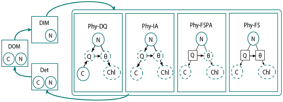
Figure 1. Schematic diagram of the FABM-NflexPD model. The Abiotic components (dissolved organic material (DOM), dissolved inorganic material (DIM), and detritus (Det) are calculated within the abiotic module (shown in the left hand side). The phytoplankton module, which simulates the dynamics of Phy_C and Phy_N, contains the four model variants: Dynamic Quota (DQ in Kerimoglu et al., 2021 this compartment is the Dynamic Acclimation variant, DA), Instant Acclimation (IA), Fixed Stoichiometry with Photoacclimation (FSPA), and Fixed stouchiometry (FS). Solid and dashed circles are the state and diagnostic variables, respectively. Symbols are defined in Tables 1, 2. Prescribed parameters in the DQ, FSPA, and FS variants are shown in solid squares. Black arrows indicate which parameters/variables affect the diagnostic and state variables (Kerimoglu et al., 2021).

2.1. Model Variants

The four model variants follow a common formulation to describe phytoplankton net growth rate (μ):

$\begin{array}{ll}\mu ={\mu }_{\text{g}}-R_{\text{Chl}}-R_{\text{N}}& (1)\end{array}$

Where μ_g, R_Chl and R_N are the cellular gross growth rate, the costs associated with chlorophyll maintenance and synthesis, and cost for nutrient uptake, respectively. Since C-fixation, which determines phytoplankton growth, occurs in the chloroplast, the gross growth rate ${\widehat{\mu }}_{\text{g}}$ and the fractional allocation of resources to the chloroplast, f_C (see below), determine μ_g:

$\begin{array}{ll}{\mu }_{\text{g}}={\widehat{\mu }}_{\text{g}}·f_{\text{C}}& (2)\end{array}$

The gross growth rate depends on the fractional day length, L_D, the potential maximum growth rate, ${\widehat{\mu }}_0$, and the light limited growth within the photosynthetic apparatus, L_I:

$\begin{array}{ll}{\widehat{\mu }}_{\text{g}}=L_{\text{D}}{\widehat{\mu }}_0{L}_{\text{I}}& (3)\end{array}$

L_I is a saturating function of daytime average irradiance Ī, the chlorophyll density in the chloroplast $\widehat{\theta }$, and the light affinity α:

$\begin{array}{ll}{L}_{\text{I}}=1-\text{exp}\left(\frac{-\alpha \widehat{\theta }\stackrel{-}{\text{I}}}{{\widehat{\mu }}_0}\right)& (4)\end{array}$

The cost of maintaining and synthesising chlorophyll, R_Chl is calculated by scaling the chloroplast-specific cost with the fractional allocation of resources to the chloroplast, f_C, which determines the growth rate. Hence, similar to μ_g (Equation 2):

$\begin{array}{ll}{R}_{\text{Chl}}={\widehat{R}}_{\text{Chl}}·f_{\text{C}}& (5)\end{array}$

The next subsection describes how specific physiological processes that contribute to phytoplankton growth are modelled across different model variants. All equations described herein are also described in Kerimoglu et al. (2021) and Smith et al. (2016).

2.1.1. Instant Acclimation (IA)

Phytoplankton are able to sustain high growth rates despite low nutrient concentration, by varying their elemental composition to produce cells that contain less of the nutrients that are in short supply. Both the IA and DQ represent this flexibility. The classical way to represent this flexibility is via the Droop (1968) quota model, where gross growth rate is calculated as a function of the nutrient quota, Q:

$\begin{array}{ll}{\mu }_{\text{g}}={\mu }_{\infty }\left(1-\frac{Q_0}{Q}\right)& (6)\end{array}$

where μ_∞, and Q₀ are the growth rate at infinite cell quota, and the subsistence cell quota at which growth becomes zero, respectively. Based on the study by Pahlow and Oschlies (2013), assuming a fixed amount of cellular nitrogen, N, is bound in the structural material (Q_s), a fraction of cellular N in excess of Q_s is allocated for nutrient uptake, as represented by f_V, and the remainder is assumed to be allocated to chloroplasts for growth (see Equation 2), as represented by f_C:

$\begin{array}{ll}{f}_{\text{C}}=1-\frac{2Q_{\text{s}}}{Q}-f_{\text{V}}& (7)\end{array}$

In turn, the quota–dependent “nutrient limitation” term in brackets in Equation (6), is replaced by f_C in our approach, as described by Equation (2).

Increasing f_V therefore decreases the gross growth rate (Equation 2), while increasing the rate of cellular nutrient uptake, V:

$\begin{array}{ll}V=f_{\text{V}}\widehat{V}& (8)\end{array}$

where $\widehat{V}$ is the protoplast specific nutrient uptake. The cost associated with nutrient uptake R_N (Equation 1), is the product of the prescribed cost of N uptake, ζ_N and V itself:

$\begin{array}{ll}{R}_{\text{N}}={\zeta }_{\text{N}}·V& (9)\end{array}$

Following Pahlow et al. (2013) the optimal cell quota, Q⁰ can be calculated as:

$\begin{array}{ll}{Q}^0=Q_{\text{s}}\left[1+\sqrt{1+\frac{1}{Q_{\text{s}}\left(\frac{{\widehat{\mu }}_{net}}{\widehat{V}}+{\zeta }_{\text{N}}\right)}}\right]& (10)\end{array}$

Thus, the optimal Q⁰ depends on the ratio of light- to nutrient-limitation ($\frac{{\widehat{\mu }}_{\text{net}}}{\widehat{V}}$). By balancing growth and uptake, μQ = V, via the balanced growth equation (Burmaster, 1979), it is possible to calculate the optimal f_V, $f_{\text{V}}^0$ (Pahlow and Oschlies, 2013):

$\begin{array}{ll}{f}_{\text{V}}^0=\left(\frac{Q_{\text{s}}}{Q}\right)-{\zeta }_{\text{N}}(Q-Q_{\text{s}})& (11)\end{array}$

where ζ_N is the cost of assimilating DIN [mol C (mol N^-1)]. Thus, f_V increases with decreasing cellular N quota, Q; i.e., more nutrient limited cells allocate more resources towards nutrient uptake, $\widehat{V}$. This process rate depends on maximum uptake rate ${\widehat{V}}_{\text{max}}$ and nutrient affinity Â:

$\begin{array}{ll}\widehat{V}=\frac{{\widehat{V}}_{\text{max}}·Â·\text{DIN}}{{\widehat{V}}_{\text{max}}+·\text{DIN}}& (12)\end{array}$

The second fractional resource allocation is towards nutrient affinity, f_A. Increasing f_A increases nutrient affinity at the expense of decreasing maximum uptake rate:

$\begin{array}{llll}Â& =& f_{\text{A}}{Â}_0& (13)\end{array}$

$\begin{array}{llll}{\widehat{V}}_{\text{max}}& =& (1-f_{\text{A}}){\widehat{V}}_0& (14)\end{array}$

Where Â₀ and ${\widehat{V}}_0$ are the potential maximum affinity and nutrient uptake rate, respectively. Substituting these assumptions to Equation (12),

$\begin{array}{ll}\widehat{V}=\frac{(1-f_{\text{A}}){\widehat{V}}_0·f_{\text{A}}{Â}_0·\text{DIN}}{(1-f_{\text{A}}){\widehat{V}}_0+f_{\text{A}}{Â}_0·\text{DIN}}& (15)\end{array}$

The optimum f_A maximises $\widehat{V}$, therefore f_A can be dynamically calculated:

$\begin{array}{ll}\frac{d\widehat{V}}{d{f}_{\text{A}}}=0\to f_{\text{A}}={\left[1+\sqrt{\frac{{Â}_0·DIN}{{\widehat{V}}_0}}\right]}^{-1}& (16)\end{array}$

Apart from changing the Nutrient:C composition to optimise their growth, phytoplankton are also able to adjust their Chl:C ratio, i.e., photoacclimate under changing light conditions. The Chl:C ratio within the chloroplast increases under low light to enhance light-harvesting efficiency, and decreases under high light to free up resources for other uses. In the IA and DQ model, this process is based on the rate of the net carbon fixation rate within the chloroplast (Pahlow et al., 2013):

$\begin{array}{ll}{\widehat{\mu }}_{\text{net}}={\widehat{\mu }}_{\text{g}}-{\widehat{R}}_{\text{Chl}}& (17)\end{array}$

$\begin{array}{ll}{\widehat{R}}_{\text{Chl}}=({\widehat{\mu }}_{\text{g}}+R_{\text{M}}^{\text{Chl}}){\zeta }_{\text{Chl}}\widehat{\theta }& (18)\end{array}$

Where ${\widehat{R}}^{\text{Chl}}$ is the cost of light harvesting within the chloroplast, $R_{\text{M}}^{\text{Chl}}$ is the cost of maintaining chlorophyll and ζ_Chl is the cost of chlorophyll synthesis.

From Equation (18), reducing $\widehat{\theta }$ will also reduce the cost of light harvesting, but will increase the light limitation, as described in Equation (3). In the IA model, $\widehat{\theta }$ adjusted instantaneously to maximise the ${\widehat{\mu }}_{\text{net}}$ (Pahlow et al., 2013):

$\begin{array}{ll}\widehat{\theta }=\{\begin{array}{cc}\frac{1}{{\zeta }_{\text{Chl}}}+\frac{{\widehat{\mu }}_0}{\alpha Ī}\left(1-W_0\left[\left(1+\frac{R_{\text{M}}^{\text{Chl}}}{L_{\text{D}}{\widehat{\mu }}_0}\right)\text{exp}\left(1+\frac{\alpha Ī}{{\widehat{\mu }}_0{\zeta }_{\text{Chl}}}\right)\right]\right),& Ī>{Ī}_{\text{C}}\\ 0,& Ī\le {Ī}_{\text{C}}\end{array}& (19)\end{array}$

where, W₀ is the 0-branch of the Lambert-W function and Ī_C is the critical daytime average irradiance level, below which it is not worthwhile to synthesise chlorophyll (Pahlow et al., 2013):

$\begin{array}{ll}{Ī}_{\text{C}}=\frac{{\zeta }_{\text{Chl}}{R}_{\text{M}}^{\text{Chl}}}{\alpha L_{\text{D}}}& (20)\end{array}$

The cellular Chl:C ratio is obtained by multiplying $\widehat{\theta }$ by the allocation of resources towards chloroplast, f_C :

$\begin{array}{ll}\theta =\widehat{\theta }·f_{\text{C}}& (21)\end{array}$

2.1.2. Dynamic Quota (DQ)

The DQ variant like the IA model, resolves photoacclimation (Equations 17–21). However, in order to make the rest of the model resemble a typical Droop model, physiological allocation factors, f_V and f_A in Equations (7, 15), respectively, are not optimised as in the IA model, but prescribed, as the biomass-weighted spatio-temporal averages of their values estimated by the IA variant.

With the assumption of fixed f_V, nutrient uptake rate for the whole cell can become unrealistically high, as DIN and hence Phy_N increase, yielding unrealistically high Q. Therefore, a down-regulation term is required to limit Q values. Following earlier examples (e.g., Morel, 1987; Grover, 1991) this is described as a liner function of the difference between a maximum prescribed quota, Q_max and the actual Q, relative to the effective capacity, given by the difference between the Q_max and subsistence quota, Q_s :

$\begin{array}{ll}{f}_{\text{Q}}=\frac{Q_{\text{max}}-Q}{Q_{\text{max}}-Q_{\text{s}}}& (22)\end{array}$

The nutrient uptake rate, V in Equation (8) then becomes:

$\begin{array}{ll}V=f_{\text{V}}\widehat{V}{f}_{\text{Q}}& (23)\end{array}$

which also affects the respiratory cost of nutrient uptake, R_N (Equation 9):

$\begin{array}{ll}{R}_{\text{N}}={\zeta }_{\text{N}}{f}_{\text{V}}\widehat{V}{f}_{\text{Q}}& (24)\end{array}$

Another important difference from the IA model is that the DQ variant tracks both N and C bound to phytoplankton (i.e., Phy_C, Phy_N) explicitly, similar to the “DA” variant in Kerimoglu et al. (2021), therefore Q becomes:

$\begin{array}{ll}Q=\frac{Ph{y}_{\text{N}}}{Ph{y}_{\text{C}}}& (25)\end{array}$

In the classical Droop approach, increasing Q to high levels yields diminishing returns in terms of growth. The DQ variant herein, with constant allocation factors as prescribed, retains the typical saturating relationship between growth rate and Q from the Droop equation, albeit somewhat flatter, as discussed in detail in the Supplementary Material. In the DQ model, Q is calculated simply as the ratio of Phy_N to Phy_N.

Kerimoglu et al. (2021) have demonstrated that the IA approach employed in a 1D setup yields results almost identical to an otherwise identical model that explicitly resolves the dynamics of C and N biomass (their “DA” variant). Therefore, the most important difference between our IA variant and this DQ control is that the nutrient vs. carbon uptake and nutrient affinity vs. maximum nutrient uptake rate are optimised only in the former.

2.1.3. Fixed Stoichiometry (FS)

The FS variant resembles the typical phytoplankton growth model based on fixed Chl:C:N as commonly used in global OBGC models (i.e., models in Le Quere et al., 2005; Laufkotter et al., 2015; Totterdell, 2019), and is the same as described by Kerimoglu et al. (2021). It describes nutrient limitation with a rectangular hyperbolic nutrient uptake function of ambient nutrient concentration (Monod, 1949):

$\begin{array}{ll}{\mu }_{\text{g}}={\widehat{\mu }}_{\text{g}}·\frac{DIN}{K_{\text{N}}+DIN}& (26)\end{array}$

Following Button (1978) and Smith et al. (2009), the half saturation value K_N can be diagnosed from the solution of the IA variant, as a function of ${\widehat{V}}_{\text{max}}$ (Equation 14) and  (Equation 13):

$\begin{array}{ll}{K}_{\text{N}}=\frac{{\widehat{V}}_{\text{max}}}{Â}=\frac{(1-f_{\text{A}}){\widehat{V}}_0}{f_{\text{A}}{Â}_0}& (27)\end{array}$

Based on this identity, K_N is calculated from the spatio-temporal biomass-weighted average of f_A, and the prescribed values of parameters ${\widehat{V}}_0$ and Â₀ used in the IA variant.

The light limitation is described by the same saturation function used in the other variants (Equation 4), but based on prescribed chlorophyll density, $\widehat{\theta }$, based on the IA run, making θ constant, as illustrated in Figure 1. In order to ensure consistency with the IA model, θ is calculated in its expanded form, based on the resource allocation towards growth (f_C) described in Equation (7):

$\begin{array}{ll}{\theta }_{\text{FS}}=\left(1-\frac{2Q_{\text{s}}}{Q_{\text{fixed}}}-f_{\text{V}}\right)·\widehat{\theta }& (28)\end{array}$

Throughout each simulation, the terms Q_fixed and f_V are set to constant values, which are their respective biomass-weighted means from the IA variant. The cellular nutrient uptake rate, V, is calculated based on the balanced growth equation (i.e., V = μ·Q_fixed) as in the IA variant.

2.1.4. Fixed Stoichiometry With Photoacclimation (FSPA)

This variant is formulated to isolate the effect of photoacclimation on model performance and response in the oligotrophic ocean. As in the FS variant, nutrient limitation is calculated using the rectangular hyperbolic function and directly determines the phytoplankton growth. However, the Chl:C ratio within the chloroplast, $\widehat{\theta }$ adjusts instantaneously via Equation (19), just as in the IA variant. Thus, similar to the FS variant, this variant uses constant values of Q_fixed and f_V to calculate the resource allocated to phytoplankton growth and hence the cellular Chl:C ratio, θ, but with time-varying $\widehat{\theta }$. The nutrient limitation and gross growth rate are calculated based on Equation (26) and its half saturation constant is approximated from the IA variant as for the FS model (Equation 27).

2.2. Simulations and Model Metrics

We simulate two oligotrophic stations with extensive time-series observations: ALOHA and BATS. In order to simulate realistic conditions with a 1-D setup, the FABM-NflexPD is coupled to the General Ocean Turbulence Model (GOTM, Burchard et al., 2006). FABM acts as an interface between the biogeochemical and hydrodynamic models, which allows switching between different model formulations (i.e., versions). The hydrodynamic model solves the advection-diffusion-reaction equations, provides physical variables, such as Ī, to the biogeochemical model, and handles the model input and output. Meanwhile, FABM provides the rate of sinking/floating of biogeochemical state variables, which are solved as residual vertical advection (Bruggeman and Bolding, 2014). For the vertical advection scheme we use the third-order TVD with ULTIMATE QUICKEST limiter, and the Runge-Kutta method for the time integration scheme with no flux boundary condition. FABM also provides feedback to physics, such as the light absorption, which is applied in this study.

As the initial conditions for the hydrodynamical model, we use in situ temperature and salinity profiles (obtained from https://hahana.soest.hawaii.edu/hot/hot-dogs/cextraction.html and batsftp.bios.edu/BATS/bottle/ for ALOHA and BATS, respectively). Meteorological forcing, from the European Centre for Medium-Range Weather Forecasts (ECMWF), ERA-5 hourly reanalysis, with horizontal resolution of 0.25^o×0.25^o (https://cds.climate.copernicus.eu/cdsapp#!/dataset/reanalysis-era5-single-levels?tab=overview), include: wind speed, air pressure, air temperature, humidity, cloud cover, shortwave radiation, and precipitation, each calculated using the Fairall et al. (1996) method. The model domain, split into 100 levels with surface zooming, extends to 500 m for ALOHA and 450 m for BATS, where some temperature and salinity profiles are limited to 450 m. To describe the background turbidity, we assume Jerlov type IA for ALOHA, based on field measurements in the North Pacific (Paulson and Simpson, 1977), and Jerlov type I for the very clear water at BATS (Kullenberg, 1984).

All model variants are run for 8 years, from 1st January 2008 to 31st December 2016. The first 3 years, as spinup period, are forced using repeating climatology, i.e., mean hourly and daily values for the meteorology, and the monthly means of observed temperature and salinity from 1st January 2008 to 31st December 2016. For the rest of the year, none of the forcings are nudged towards the observation (analytical method in GOTM = 1). The last 5 years of model output is compared with observations of Chl from HPLC, DIN (Nitrate + Nitrite), and PP, which are the most widely observed variables that are commonly compared to model outputs (Mongin et al., 2006; Kwiatkowski et al., 2014; Chen and Smith, 2018a). Of the widely available observables, these three are also the most directly related to the biogeochemical impacts of variable phytoplankton composition. These observations can be obtained from http://batsftp.bios.edu/BATS/bottle/ and https://hahana.soest.hawaii.edu/hot/hot-dogs/bextraction.html, for BATS and ALOHA, respectively. Observed Chl, DIN, and PP are used to tune the model variants.

In order to thoroughly assess how well each model variant captures the observations, and its portability (i.e., applicability to different sites without re-tuning parameter values), we perform three experiments: (i) the reference simulations of each station with individually tuned parameter sets (model runs labelled IA, FS, FSPA, and DQ); (ii) cross-validation, where phytoplankton-related parameters tuned for station ALOHA are applied at station BATS and vice versa, (model runs labelled IA-X, FS-X, FSPA-X and DQ-X); and (iii) simultaneous runs using a common parameter set for phytoplankton-related processes at both stations, (labelled IA-S, FS-S, FSPA-S, and DQ-S). For experiments (ii) and (iii) initial conditions and some abiotic parameters, such as sinking speed and detrital degradation rate, are kept the same as experiment (i) for each station. The choice of parameters for these three experiements are described in section 2.3. We quantify model performance in terms of statistical metrics (i.e., correlation, bias, and RMSE) and a weighted cost function for overall mismatch between models and observations.

The cost function is computed as the weighted average of the squared difference between observed and simulated values, using the sample standard deviation of all observations of type m, ${\widehat{\sigma }}_m$, to appropriately weight the contribution of each model-data misfit, as in previous studies (e.g., Friedrichs et al., 2006; Hemmings and Challenor, 2012; Kaufman et al., 2018). However, because the variables that we compared tend to be distributed log normally, especially at depths where their concentration are high, we use a square-root transformation to calculate the model data difference (Dadou et al., 2004; Hemmings and Challenor, 2012). Thus, the total cost function becomes:

$\begin{array}{ll}{J}_m=\frac{C_m}{N_m}{\displaystyle \sum _{j=1}^{N_m}}\frac{1}{{\widehat{\sigma }}_m}{\left(\sqrt{a_{jm}}-\sqrt{{â}_{jm}}\right)}^2& (\mathrm{29a})\end{array}$

$\begin{array}{ll}J=\frac{1}{M}{\displaystyle \sum _{m=1}^M}{J}_m& (\mathrm{29b})\end{array}$

Where M is the number of variable types (M= 3; Chl, DIN, and PP), N_m is the number of observations of type m, and a_jm and â_jm are the modelled and observed values, respectively. The term C_m in Equation (29) is included to enhance the weight of DIN compared to the cumulative weight of the other two phytoplankton-related variables that we evaluate, by setting C_m = 1 for Chl and PP, and C_m = 2 for DIN. All variables are evaluated at their observed time and depth. We quantify model portability in terms of the portability index (PI, Friedrichs et al., 2007) which is the ratio of total costs (Equation 29b) from simultaneous experiment (J^s) and the cross-validation (J^x) experiment:

$\begin{array}{ll}\text{PI}=J^s/J^x& (30)\end{array}$

PI values approaching unity indicate increasing portability.

2.3. Parameter Fitting

As explained in the introduction, this study explores how phytoplankton growth formulation affects model performance. Based on initial model runs, we adjust three parameters separately for each stations: ${\widehat{\mu }}_{\text{0}}$, k_det, and k_DON. We choose a slightly lower value for ${\widehat{\mu }}_{\text{0}}$ at station ALOHA, since Chl concentration at ALOHA is lower than BATS (Saba et al., 2010) and this yield better results in terms of statistical metrics compared to using the same ${\widehat{\mu }}_{\text{0}}$. A higher k_det and lower k_DON are also applied in this station to prevent the depletion of DIN near the surface during the simulations. Mortality, M_p, and the fraction thereof that becomes detritus, M_part, as well as other abiotic parameters are kept constant for all model variants at both stations. These parameters are described on Table 1.

TABLE 1

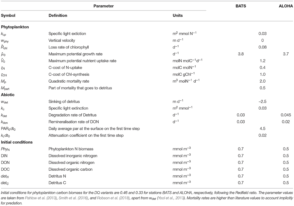
Table 1. Common parameter values for simulations of stations ALOHA and BATS for all model variants.

In order to ensure a fair comparison, we systematically tune the two parameters, separately for each variant, that most directly affect phytoplankton growth, α^I and Â₀, respectively such that each model variant attains its best performance at each station. This is achieved through an analysis of the response surface of model skill for each variant, respectively. This analysis also reveals how perturbing the parameters affects the model performance, in terms of simulating the biogeochemical variables (Chl, DIN, and PP), as well as the overall model-data agreement, as quantified by the cost, for each station. The parameter ranges were made as wide as practically possible, up to the limits for which solutions can be obtained. Thus, the parameter values explored for α^I space, are 2.0, 2.5, 3.0, 3.5, 4.0, 4.2, and Â₀ space are 0.07, 0.1, 0.3, 0.5, 0.7, 0.9, 1.1, and 1.3, resulting in 48 model simulations per variant per site. The combination of parameter values giving the lowest overall cost for each station is used in the reference simulation and cross validation experiments (running the model at BATS using the parameter set that has the lowest cost for ALOHA, and vice versa). The combination which give the lowest total cost for both stations (J_BATS + J_ALOHA) is used for the simultaneous experiment (see section 2.2). The chosen parameters for these experiments are summarised on Table 2. To better understand the effect of parameter variations, we plotted the landscapes of component costs (for each observable) and the overall cost obtained over the range of parameter values.

TABLE 2

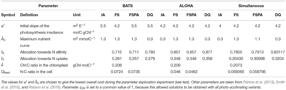
Table 2. Parameterst values tuned based on stations and model variants.

To summarise, we perform three experiments: individual tuning, cross validation, and simultaneous using four different model variants, IA, FS, FSPA, and DQ models. Short descriptions of these experiments can be found on Table 3.

TABLE 3

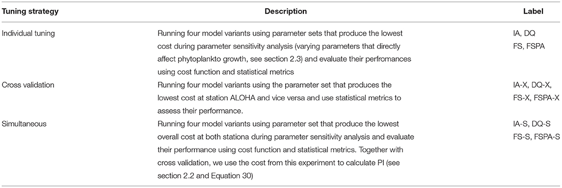
Table 3. Summary of experiments perform in this study.

3. Results

3.1. Model Skill Response Surfaces

Previous studies have shown that optimising fewer than 10 parameters tends to yield better predictive skill for models (Friedrichs et al., 2006; Ward et al., 2013). In this study, we choose to vary the two most important parameters that determine the overall phytoplankton growth response under oligotrophic conditions: the light and nutrient affinities, Â₀ and α^I, respectively. Apart from identifying the most suitable parameter combinations to be applied at different stations for each model variant, exploring this parameter space allows us to investigate how different phytoplankton acclimation formulations respond to parameter perturbations. Model skill response surfaces (Figure 2) suggest two distinct regions: where all model variants show relatively low costs (Â₀ > 5.0 and α^I > 2.5), and where the cost increases steeply, especially at low Â₀. Variants lacking variable Q especially suffer in this cost region. Despite the FSPA variant allowing photoacclimation, the cost associated with low Â₀ and low α^I is similar to that in FS model. However, adding photoacclimation lowers the cost associated with perturbing α^I, especially in the “low” cost region, to values even lower than for the variants that include both Q and photoacclimation (Figures 2A,C,D). Variants with variable N:C and Chl:C have flatter overall cost landscapes; when combining low Â₀ and low α^I, the costs for both IA and DQ models are further reduced when Â₀ = 0.3 and α^I < 4.0, although cost still increases for low α^I and Â₀ > 0.5.

FIGURE 2

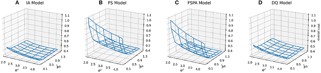
Figure 2. Mesh plots of overall cost, combined for both stations for the four model variants: IA, FS, FSPA, and DQ (A–D) as a function of the nutrient affinity (Â₀) and light affinity (α^I, Chl specific slope of the PI curve) parameters.

The most striking difference between the fixed stoichiometry and variable Q groups are the shapes of their cost landscapes for both non-phytoplankton (DIN) and phytoplankton-related variables (Chl and PP, Figure 3). In terms of DIN, when Â₀ < 0.7, models with fixed stoichiometry show a dramatic increase in DIN cost, and for the variants that include variable Q, cost increases for Â₀ < 0.5. For Chl, these variants show an opposite pattern compared to DIN, where cost decreases with decreasing Â₀, with the DQ model producing higher cost and steeper landscape compared to the IA model (Figures 3E,H). Conversely, the fixed stoichiometry variants produce similar patterns for Chl and DIN costs, with a sharp increase in cost for Â₀ < 0.1, especially in the FS variant (Figure 3F). Inclusion of photoacclimation in the FS model reduces the Chl and PP costs, especially in the lower cost region (Â₀ > 0.5, and α^I > 2,5, Figure 3G), or when both Â₀ and α^I are low. For most of the model variants, the cost landsapes are similar for PP and Chl. However, compared to Chl, the PP cost increases less steeply with decreasing α^I in the DQ model (Figure 3L), while the IA model shows a slight increase in PP cost with increasing α^I (Figure 3I). The FS and FSPA models show similar tendency in terms of the cost landscape, although the latter produces slightly lower cost. The FS and FSPA variants also show shallow declines in PP cost with decreasing Â₀, but sharp increases for Â₀ > 0.1. For these variants, with nutrient affinity near the low end of its range (Â₀ = 0.07), PP cost declines sharply with increasing α^I.

FIGURE 3

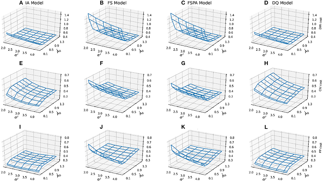
Figure 3. Mesh plots of the component costs for each observable, combined for both stations, by row: DIN (A–D), Chl (E–H), and PP (I–L) as a function of the nutrient affinity (Â₀) and light affinity (α^I, Chl specific slope of the PI curve) parameters. Costs for model variants by column: IA (A,E,J), FS (B,F,J), FSPA (C,G,K), and DQ (D,H,L), respectively.

In summary, for the overall cost, all variants follow a similar pattern, but with less steep increases in cost as either α^I and Â₀ decreases in variable Q models (IA and DQ). The variable Q models also generally produce flatter cost surfaces, both for the overall cost and its components, compared to only accounting for photoacclimation. Nevertheless, photoacclimation alone generally improves both overall and variable-specific costs.

3.2. Performance of the Three Variants

In oligotrophic regions, summertime nutrient concentrations are typically < 0.01 mmol m⁻³ within the euphotic zone (Steinberg et al., 2001; Anderson and Pondaven, 2003; Dave and Lozier, 2010), with vertical stratification that is destroyed by deep mixing during winter and spring (Dave and Lozier, 2010). All model variants capture these characteristics well, as seen in the DIN distributions (Figures 4F–I, 4U-X, 5I-P, 6C,D). At station BATS, winter mixing typically increases DIN from ~ 0.05 to 0.5 mmol m⁻³ (Figure 4J), as captured by all model variants, but exaggerated by the IA and DQ (Figures 4F,I). At BATS all variants overestimate the average winter time DIN within the upper 50m (Figure 6C), but the IA underestimates the DIN concentration in the summer. All variants also overestimate the winter DIN concentration at ALOHA in the upper 50 m, but capture the summer-autumn concentrations (Figure 6D). However, at 75–125 m between summer and autumn the four variants are more similar, with the DQ variant producing slightly higher DIN than other variants, especially during summertime (Figures 5M–P, 6G,H). Although all model variants realistically capture DIN concentration and seasonality in the upper 50 m (Figures 4U–Y), none captures the sporadic spikes of DIN that occur at both stations (Figures 6G,H).

FIGURE 4

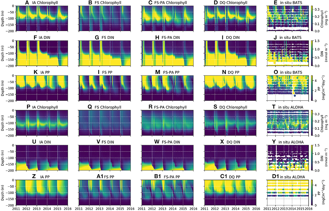
Figure 4. Contour plots of observables by row: Chl, DIN, and PP, at stations BATS (upper panels, A–O) and ALOHA (lower panels, P–D1) from 1st of January 2011 to 31st December 2015, for each of the model variants, by column, and the in-situ time-series observations (right-most column).

FIGURE 5

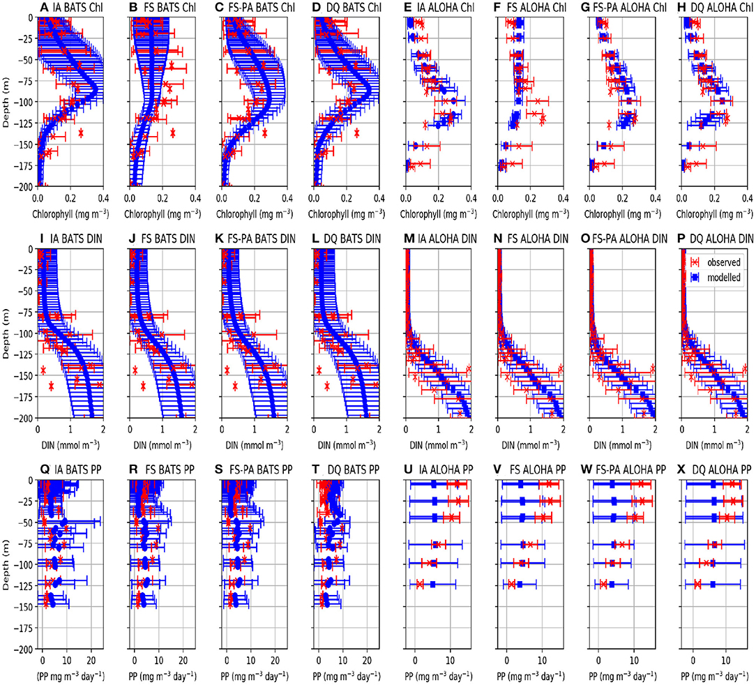
Figure 5. Vertically averaged values of modelled (blue) and observed (red) Chl, DIN, and PP from 1st January 2011 to 31st December 2015. The error bars represent the standard deviation of the biogeochemical variables. Profiles for station BATS are shown in (A–D,I–L,Q–T), for Chl, DIN, and PP respectively. For station ALOHA, profiles are shown in (E–H,M–P,U–X), for Chl, DIN, and PP respectively.

FIGURE 6

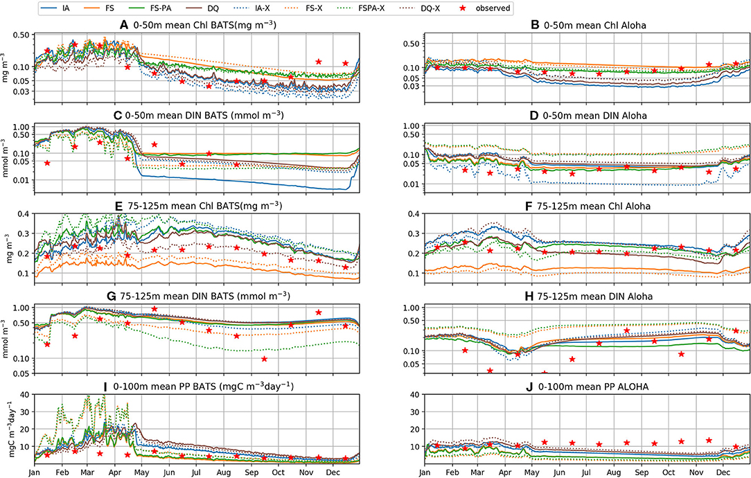
Figure 6. Depth averaged [upper 50 m (A–D), and between 75 and 125 m (E–H)] Chl, DIN, and PP for the period of 1st January 2011 to 31st December 2015, for the IA (blue), FS (orange), FSPA (green), and DQ (brown) model variants respectively. Solid lines: individually tuned runs; dash-dot lines: cross-validation experiments; red stars: monthly averaged in situ DIN, Chl, and PP measurements. The upper 50 m is most consistently stratified, and the nutricline and SCM usually occur from 75 to 125 m. PP was averaged over the upper 100 m, where PP is > 3 mgCm⁻³ day⁻¹, shown in (I,J).

Similar to DIN, Chl in the oligotrophic region is typically scarce in the euphotic zone due to nutrient limitation. Between 50 and 200 m depth, where nutrients are more abundant, subsurface Chl maxima (SCM) occur during summer (Dave and Lozier, 2010; Mignot et al., 2014). All variants capture these characteristics qualitatively well, both seasonally and vertically at BATS (Figures 4A–E). However, at ALOHA the FS variant is unable to simulate low Chl in the upper 100 m, nor distinct summertime SCM profiles (Figures 4Q, 5R) as shown in the observation (Figure 4T) and other variants which allow variable cell quota (Figures 4P,S). The inclusion of photoacclimation, in the FSPA model, results in better simulation of Chl profile, with low concentration in the upper 100 m and summertime SCM profiles (Figures 4C,R), despite simulating slightly deeper and lower concentration of DCM at BATS and ALOHA, respectively, compared to IA and DQ, (Figure 5C). All model variants capture typical Chl concentrations and seasonality for the SCMs that usually occur between 75 and 125 m at both stations (Figures 5A–D, 6E). However, when averaged vertically, the IA variant tends to overestimate Chl concentrations compared to other variants (Figures 5A, 6E). This result differs from Ayata et al. (2013), where all models underestimated SCM concentrations, except during blooms. Although the IA and DQ variants are qualitatively similar at BATS, generally the latter simulates slightly lower Chl and shallower SCMs at both stations, compared to the IA variant (Figures 4A,D). Comparing all model variants, from 75 to 125 m, the FS variant produces the lowest Chl because it lacks flexible quota, but the FSPA variant produces a similar range of averaged Chl concentration as IA and DQ, more similar to the former during summertime (Figures 6E,F). Despite capturing the DIN concentration in the upper 50 m, neither the DQ nor IA variant captures Chl from summer to winter at ALOHA (Figures 6B,D). The FS and FSPA perform somewhat better in this regard, but still overestimate summertime Chl at BATS (Figures 6A,B).

Unlike Chl and DIN, PP distributions in oligotrophic regions are usually skewed towards the surface and limited to the upper ~120 m (Dave and Lozier, 2010). All variants capture the PP depth and its decline during summer at BATS, but with higher PP and later peaks than observed (Figures 4K–N, 6I). Compared to the observations and other variants, the FS variant produces briefer spikes of higher PP (>20 mgC m⁻³ day⁻¹). The inclusion of photoacclimation prolonged the spikes of PP and deepened its summertime distribution to depths deeper than the IA and DQ models (Figures 4M,B1). When averaged horizontally, the variants with variable Q generally capture well observed PP (Figures 5Q,T,U,X) especially at BATS, but the FS and FSPA underestimates PP in the top 50 m, particularly during summer. The IA and DQ variants simulate a slight increase in PP at ~50 m, slightly deeper than its observed depth of ~60 m (Figures 5Q,T). Unlike BATS, PP at ALOHA peaks in the summer, and declines in spring (Dave and Lozier, 2010), with the highest rate recorded in the upper 50 m, decreasing with depth (Figures 5U–X). None of the variants completely capture these patterns, especially the FS and FSPA variants which consistently underestimate PP in the upper 50 m (Figures 6J, 5V,W), but the IA and DQ do capture winter and spring PP rates at ALOHA. The DQ variant produces generally the highest PP, which may be because it produces the highest C:N ratio (lowest Q) within the top 100 m and therefore agrees best with the observations at ALOHA (Figure 6J).

The Taylor and target diagrams (Jolliff et al., 2009) shown in Figures 7, 8 and cost values (J_m, J) listed in Table 4 summarise the skills of model variants for all experiments. In general, the models perform similarly for DIN, but differ more for Chl and PP. At BATS, the statistical metrics from the latter two show some disparity in terms of standard deviations (Figures 8B,C), which are also reflected by their RMSDs in the target diagrams (Figures 8E,F). At the more stable station ALOHA, the statistical metrics differ more among the model variants.As seen from Table 4, the FSPA variant produces the lowest overall (Figure 2B), Chl (Figure 3B), and DIN (Figure 3F) costs for the individually tuned runs, as reflected in the overall cost landscape regions for high Â₀ and α^I (Figure 2C). The FSPA variant also produces the lowest Chl RMSD and bias. The absence of photoacclimation in the FS model produces the worst overall Chl, and PP costs as well as correlation and RMSD. Based on Table 4, The 'second best' model in terms of overall cost, is the IA model, which produces the lowest PP cost, RMSD, and bias, as well as the highest Chl correlation. The DQ performs slightly worse than the IA model in terms of cost (Figures 7, 8, and Table 4), however it produces the best correlation for PP, and generally performs similarly to the IA model.

FIGURE 7

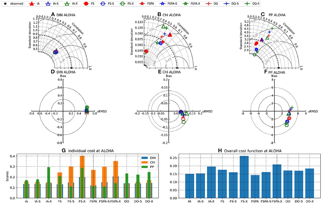
Figure 7. Taylor (A–C), target (D–F) diagrams (μRMSD is normalised RMSD), and costs (G,H) for Chl, DIN, and PP at station ALOHA for the IA (triangles), FS (circles), FSPA (stars), and DQ (cross) variants, each tuned individually to the observations (red), cross-validated (blue), and simulating both stations with a common parameter set (green). The cost functions J_m (G) and J (H) were calculated for the individually tuned runs, cross validation experiment (-X suffix) and the simultaneous experiment using a common parameter set (-S suffix), for each model. Values for J_m, J and PI are provided on Table 4.

FIGURE 8

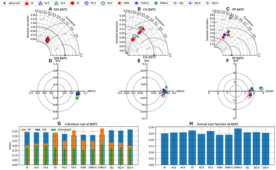
Figure 8. Same as Figure 7, but at station BATS.

TABLE 4

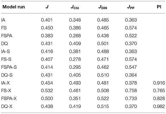
Table 4. Cumulative costs J_m for Chl, DIN, and PP (J_Chl, J_DIN, and J_PP, respectively) and J at stations ALOHA and BATS for each model run, and portability index PI (=J^s/J^x).

3.3. Model Portability

The cross-validation experiment tests a model's ability to reproduce observations from different regions without tuning, and therefore its predictive ability (Friedrichs et al., 2006). In this experiment, all model variants differ only slightly in their statistical metrics for DIN, compared to the individual tuning. However, for Chl and PP, using the parameter set tuned for a different station generally increases cost, RMSD, and bias, while reducing correlation for all variants (Figures 7A–F, 8A–F). In the cross-validation experiment the FS and FSPA variants' statistical metrics suffer most, especially in terms of PP, where both variants greatly overestimate and underestimate the winter and seasonal values at BATS and ALOHA, respectively (Figures 6I,J). For the IA and DQ variants, the cross validation and individually tuned results differ only slightly from the observations and often capture the observations when the reference simulations do not, especially at BATS during summer within the upper 50 m (Figures 6A,B). However, at 75–125 m, the cross validations from IA often overestimate greatly the observed Chl at BATS and ALOHA (Figures 6E,F), while the DQ variant captures the observation well at BATS, but also overestimates the Chl at ALOHA. In terms of cost, the DQ variant produces the lowest discrepancy between the reference and cross validation simulation (ΔJ= 0.0043).

The simultaneous experiment evaluates the potential applicability of each model variant at multiple stations with a common parameter set, as in a typical global or regional biogeochemical model (Friedrichs et al., 2007). The simultaneous tuning is done by choosing the parameter set that yields the lowest overall cost, summed over both stations (J_BATS+J_ALOHA). This experiment yields relatively similar J values and statistical metrics, although the results are slightly worse in terms of J, except that for the FS and DQ variants the simultaneous runs performed better than the reference, which is most apparent for ALOHA (Figures 7B,C,E,F). As discussed in Friedrichs et al. (2007), the ideal model would have a PI ~1 (Equation 30), indicating good performance at multiple sites without being tuned individually for each, while also having a low cost. Figures 7G,H, 8G,H reveal that in general photoacclimation greatly improves model performance, especially for Chl and DIN, and enhances portability. The inclusion of variable Q in combination with photoacclimation (IA and DQ models) yields even better performance in terms of PP and portability, at least between these oligotrophic sites. Although the fixed stoichiometry with photoacclimation (FSPA) model produces the lowest overall cost in both the reference and simultaneous experiments, its poor performance in the cross validation experiment indicates that it is less portable compared to the IA and DQ models. From Table 4 the DQ is the most portable, however in terms of the average cost over all experiments, the IA variant produces slightly lower cost (average costs for DQ and IA are 0.434 and 0.424, respectively), indicating that the DQ model is the most portable. However, compared to the DQ model, the IA model produces nominally better RMSD and bias for all observables in both cross validation and simultaneous experiments, despite having fewer state variables.

4. Discussion

The Chl:C:nutrient ratios of phytoplankton vary as a result of both evolutionary adaptation, which has produced a variety of species and strains of different compositions, and physiological acclimation, which dynamically alters the composition of many species (Smith et al., 2011; Moreno and Martiny, 2018). However, many large-scale OBGC models assume constant elemental and pigmentary composition for phytoplankton (Bopp et al., 2013; Laufkotter et al., 2015), similar to the FS approach herein. Some models resolve diverse phytoplankton communities by explicitly accounting for as many as hundreds of differently adapted types (Follows and Dutkiewicz, 2011), and a few account for inter-specific differences in composition (Dutkiewicz et al., 2019). Others represent these flexibilities in terms of physiological acclimation, typically using a Droop quota model (e.g., Moore et al., 2001), but seldom with a more consistent allocation framework in large-scale OBGC models (Kerimoglu et al., 2017; Kwiatkowski et al., 2018; Pahlow et al., 2020). A few studies have even resolved variable composition for a diversity of phytoplankton types (e.g., Blackford et al., 2004; Ward et al., 2014; Butenschon et al., 2016). All of these approaches typically require additional state variables and calculations and therefore when applied to multiple phytoplankton functional types can be computationally expensive, as demonstrated by Kwiatkowski et al. (2014). To overcome these problems, at least for acclimative models, Smith et al. (2016) proposed the IA approach, which optimises Chl:C:nutrient ratios instantaneously for local conditions, so that variable composition can be tracked via a single state variable (biomass).

We have recently demonstrated that the IA approach behaves similarly to the fully dynamic version (DA) in a spatially explicit 1D setup (Kerimoglu et al., 2021). Here we assess four different models for phytoplankton growth against in-situ observation at two oligotrophic stations with different physical conditions. Comparing the FS, FSPA, DQ, and IA models, which differ in their degrees of flexible composition and computational efficiency, has allowed us to disentangle the impact of different aspects of acclimative response on model performance and portability.

4.1. Cost Landscapes

The steep increase in cost with decreasing nutrient affinity for the FS and FSPA variants reveals their greater sensitivity, compared to the DQ and IA variants. This is because with the Monod formulation used in the FS and FSPA models, growth rate depends directly and immediately on the ambient nutrient concentration and the nutrient affinity, Â₀, which determines nutrient uptake rate at low nutrient concentrations (Button, 1978; Healey, 1980; Smith et al., 2014). For the IA and DQ models, changes in Â₀ do not so directly alter growth rate, because growth depends on the variable cell quota, Q. It has long been appreciated that internally stored nutrients, in excess of immediate requirements for growth, allow sustained growth under low ambient nutrient concentrations in temporally (Grover, 1991) or spatially (Kerimoglu et al., 2012) heterogeneous environments.

Previous studies have found that, compared to variable quota models, Monod-type models are more sensitive to fluctuations in nutrient supply, even in nutrient-replete regions (Cerco et al., 2004; Pauer et al., 2020). In low-nutrient regions, variations in nutrient supply (or affinity) would be expected to have even greater impact on growth rates, because of the typically saturating response for nutrient uptake (Button, 1978; Healey, 1980; Smith et al., 2014). The similar cost landscapes for DQ and IA models reveal that the IA model captures this storage effect despite its instantaneous adjustment of Q (hence C:N ratio). One reason for this is that the IA model's optimal resource allocation scheme compensates for low Â₀ values by increasing the fractional allocations of intracellular resources towards nutrient uptake broadly (f_V), and affinity specifically (f_A). The decoupling of growth rate from ambient nutrient concentrations may explain why the DQ and IA variants yield higher overall cost for the reference and simultaneous runs, compared to the FSPA model; i.e., regions where J_DIN is high coincide with regions where J_CHL and J_PP are low. However, since these models have flatter overall cost landscapes, their costs differ less between the simultaneous and cross validation experiments (i.e., they are more portable), compared to the FS and FSPA models.

4.2. Model Performance With Individual Tuning

With parameters tuned individually for each station, compared to the FS variant, the photo-acclimative variants capture better common features in the oligotrophic ocean, such as the depletion of DIN and Chl in the summer, near-surface primary production, and deep SCM (Mongin et al., 2006; Mignot et al., 2014; Kavanaugh et al., 2018). Even with data-assimilation, models that have fixed stoichiometry are unable to reproduce these features (Schartau et al., 2001; Ayata et al., 2013; Ward et al., 2013). Because the FS variant cannot adjust its internal composition, i.e., decrease its Chl:C during the stratified summer, it often overestimates near-surface Chl and DIN, and underestimates SCM concentrations. Additionally, the lack of variable Q in the FS and FSPA variants limits their ability to capture continuously high PP through summer, as observed. This is because with the Monod formulation used in these models, growth and PP are directly proportional to nutrient uptake rate, and therefore decline instantaneously with ambient DIN. The four variants differ most in terms of Chl between 75 and 125 m, especially at ALOHA, where the optimal physiological acclimation in the IA variant sustains growth and hence higher biomass and Chl, with higher C:N ratio (lower Q) than the DQ during summertime nutrient depletion (Figures 6E,F). The FSPA model also captures the sustained high summer Chl concentration at the DCM, because it uses fixed Q from the biomass-averaged Q obtained from the IA model. Nevertheless, compared to the FS model, the addition of only photoacclimation in the FSPA variant indeed improves the overall model performance, yielding the lowest overall cost, especially in terms of DIN and Chl, when tuned separately for each station. This improvement in model performance may be because of the lack of variable cell quota which causes a lag in nutrient consumption, therefore consuming more nutrients and producing more Chl nearer the surface (thus capturing the observations better, as shown in Figures 6B,D). However, this hinders the model's ability to capture the seasonality of PP, which depends on Phy_C as calculated from the cell quota.

A more thorough assessment of the realism of the model variants under consideration could in principle include a comparison of modelled POC:PON ratios against in situ observations (as in, e.g., Mongin et al., 2006), but that would require modelling a variety of other processes that alter the composition of detritus (e.g., digestion, excretion and detritivory by zooplankton, and differential degradation by bacteria), which would add considerable uncertainties and complicate the interpretation of model results. As a more direct alternative, it may soon be possible to compare model results against single-cell or species-level observations of cellular composition, which have only recently become available for certain types of phytoplankton in selected regions (e.g., Lopez et al., 2016; Baer et al., 2017).

In terms of PP, both the IA and DQ variants produce lower costs than the fixed quota variants. Although the FSPA variant performs substantially better than the FS in terms of Chl, it does not allow variable Q (hence, N:C), which limits its ability to capture the seasonality of PP. Additionally, inclusion of optimal resource allocation, as represented by the IA variant, indeed improves the simulation of PP, although the DQ variant captures better the maintenance of high PP during summer (Figures 4K,N,Z,C1), resulting in better PP cost at ALOHA than BATS. This may be because the DQ variant produces lower Q when μ is high due to the prescribed f_V as well as its flatter μ vs. Q curve compared to the IA variant (see Supplementary Material), which smooths the transition between 'bloom' time and non-bloom times, as shown in the observed PP (Figures 4L,X, 6I,J). Compared to the DQ model, the IA assumption constrains variations of Q more narrowly, which limits its ability to capture the storage effect. This is one reason why the IA model produces less Phy_C (Kerimoglu et al., 2012, 2021), and therefore PP, compared to the DQ model. In effect, the IA assumption restricts luxury uptake in order to allow faster growth immediately under nutrient-replete conditions (Kerimoglu et al., 2021), which can yield slower growth under subsequent nutrient scarcity compared to models that resolve more internal storage. This may also explain why the IA model overestimates Chl concentrations near the DCM.

Although almost all variants realistically simulate near-surface DIN (Figure 6D) and elevated PP in spring, none captures the typical increase between May to August (Dave and Lozier, 2010) in the North Pacific Subtropical Gyre. This discrepancy may be due to the absence of nitrogen fixers in NFlexPD (Dore et al., 2008; Church et al., 2009; Böttjer et al., 2017) and nanophytoplankton, such as Prochlorococcus (Jiang et al., 2021), which despite being low in actual biomass, can contribute up to 40% in terms of PP (White et al., 2015; Kavanaugh et al., 2018). Indeed, it would be technically straightforward to extend the model with additional phytoplankton (or zooplankton) types, which may improve these results. However, as mentioned in the introduction, this would over-complicate the interpretation of the impacts of phytoplankton growth formulations, and their differing responses to parameter perturbations and physical settings (ALOHA vs. BATS). For this reason, we prefer to keep the model configuration as simple as possible in the current study. The lack of sporadic mixing, which lifts the thin layer of Chl towards the surface (Dore et al., 2008) and other processes, such as anticyclonic eddies or effects of El-Nino (Church et al., 2009; Kavanaugh et al., 2018) that are not well simulated by the 1D physical model may also be reasons for our underestimated PP values. The in situ PP measurements, based on¹⁴C incubations at both stations (Letelier et al., 1996; Steinberg et al., 2001), are also known to result in inaccurate PP values, including over-estimates in the presence of slow-growing species (Pei and Laws, 2013, 2014), and it is unclear whether they measure net or gross PP (Marra, 2009; Kavanaugh et al., 2018).

4.3. Model Portability

The physiological acclimation, which aims to optimise growth rate in the IA and DQ variants, is similar to dynamic optimisation of parameter values (e.g., Mattern et al., 2012), as is typically applied to capture complex adaptive behaviours in response to environmental changes (Arhonditsis and Brett, 2004), e.g., physiological plasticity or succession of plankton groups (Follows and Dutkiewicz, 2011). It is therefore expected that the IA variant, which continually re-allocates resources to optimise growth, would capture better DIN and Chl dynamics at both stations in the cross-validation and simultaneous experiments. Although earlier studies (Friedrichs et al., 2007; Kriest et al., 2012; Ward et al., 2013) found that increasing model complexity does not necessarily improve misfits or predictive capability, here we found that the inclusion of photoacclimation improves the model portability. That is, the more “complex” acclimative models overall perform better compared to the simpler FS variant. However, a previous study from Ward et al. (2013) showed that with objective parameter tuning, a biogeochemical model is sufficient to capture the observation without photoacclimation at the temperate North Atlantic. A future investigation including data assimilation would provide a more thorough and conclusive assessment of how the different aspects of photoacclimation impact model performance and portability at both temperate and oligotrophic stations.

As explained in subsection 4.1, the DQ and IA variants differ least between the simultaneous and cross validation experiments, and therefore are the two most portable. However, because for the DQ model the same value of Â₀ is applied for BATS and ALOHA, its cost varies less with α^I than with Â₀. Therefore, in this particular experiment the DQ model is more portable than the IA variant. However, the IA variant generally produces better statistical metrics for all the observed variables than the DQ model. Thus, when applied to a 3D regional OBGC model, for oligotrophic regions, the IA variant can be expected to more realistically capture phytoplankton growth, nutrient uptake, and chlorophyll concentrations with fewer state variables.

4.4. Future Outlook

This study shows that adding photoacclimation improves model performance at two oligotrophic stations, and adding variable phytoplankton C:N makes models less sensitive to parameter perturbations, especially those related to affinity, and therefore improves portability. The sensitivity analysis could in future be expanded by perturbing other parameters, such as mortality and potential maximum growth, which are directly linked to phytoplankton biomass. The portability experiment could be extended by applying data assimilation to fit each model variant to the observations, as done previously in a 0-D setup (Smith et al., 2016), and by performing cross validation experiments between more contrasting (e.g., subpolar and subtropical) regions. Although both the IA and DQ variants capture Chl, PP, and DIN concentrations fairly well, the idealised models presented herein are too simplistic to fully capture oligotrophic ecosystem dynamics. Multiple plankton types inhabit oligotrophic regions, including zooplankton (Dave et al., 2015) and N-fixers (Dore et al., 2008; Karl et al., 2012) as well as other nutrients, such as phosphate (Steinberg et al., 2001; Karl et al., 2012); but our models only represent one type of phytoplankton and nutrient. Adding predation or another trophic level, depending on the grazing formulation, may change the depth of the DCM, and may also change the timing and magnitude of phytoplankton blooms (Anderson et al., 2010). However, how this may change the portability remains an open question. Three dimensional modelling studies will be required to evaluate the impacts of physical processes such as mesoscale eddies and inter-annual variations driven by El-Nino/La-Nina events, which our 1-D setup cannot capture. For more comprehensive OBGC model applications, it will also be essential to trace C, O₂, and alkalinity (Kwiatkowski et al., 2014).

Behrenfeld et al. (2016) showed that across most of the ocean variations in Chl, the most widely observed metric of phytoplankton, result more from physiological acclimation than from variations in their biomass. Models that account for photoacclimation can help to disentangle the mechanisms underlying observed Chl variations. In a broader sense, although the effects of physiological acclimation and evolutionary adaptation can in many cases be modelled with the same mathematical approaches (Smith et al., 2011), they can be expected to have distinct effects on large scale chlorophyll distributions and biogeochemistry (Moreno and Martiny, 2018). Disentangling their relative contributions remains a formidable challenge, which will require resolving explicitly both intra- and inter-specific variability in models. Our results suggest that for such purposes, the IA approach may be useful to reduce the massive computational cost of resolving acclimation processes for many phytoplankton types.

5. Conclusions

We test an NPD-type model with four different variants differing with respect to phytoplankton flexible composition and acclimative response: A Monod-type variant with fixed stoichiometry (FS), an improved monod-type variant with photoacclimation (FSPA), a variant with both variable composition using a classical Droop-quota approach and photoacclimation (DQ), and finally the Instantaneous Acclimation (IA) variant. We assess whether adding variable composition and acclimation can enhance generality and portability at two oligotrophic stations BATS and ALOHA. Additionally, we conduct a sensitivity analysis to explore how different phytoplankton growth formulations respond to parameter perturbations, especially those related to nutrient and light affinity. When individually tuned, we find that FSPA model captures Chl and DIN observations at both stations better than the other three variants, but the DQ and IA variants with variable C:N and Chl:C ratios capture the observed PP better and are less sensitive to parameter perturbations. Therefore, flexible composition and photoacclimation can be expected to enhance portability and hence potential applicability at large scales. The addition of optimal resource allocation slightly enhances model performance as quantified by statistical metrics. However, the DQ model, which calculates the dynamics of phytoplankton C and N explicitly, is more portable than the IA approach. It should be noted that these experiments are done without any formal parameter optimisation and limited to oligotrophic sites. Further studies using objective optimisation (data assimilation) and including more contrasting regions would provide a more comprehensive and thorough assessment.

Data Availability Statement

The salinity and temperature data to force the model and compare modelled and observed DIN at BATS is available at http://batsftp.bios.edu/BATS/bottle/. Data to compare Chl and PP outputs are available at: http://batsftp.bios.edu/BATS/bottle/bats_pigments.txt and http://batsftp.bios.edu/BATS/production/bats_primary_production.txt, respectively. For station ALOHA salinity and temperature data are available at: https://hahana.soest.hawaii.edu/hot/hot-dogs/bextraction.html. Data to compare modelled Chl and DIN are available at https://hahana.soest.hawaii.edu/hot/hot-dogs/bextraction.html and for PP is available at: https://hahana.soest.hawaii.edu/hot/hot-dogs/ppextraction.html. The version of NFlexPD model code used for this manuscript is stored at: https://doi.org/10.5281/zenodo.4761937.

Author Contributions

PA performed the model runs, analysed the outputs, and prepared the figures. All authors designed the study and contributed equally to the writing of the manuscript.

Funding

PA, SS, and OK are funded jointly by the Japan Society for the Promotion of Science, JSPS (P.I: SS) and German Research Foundation DFG (grant no. KE 1970/2-1, P.I.: OK).

Conflict of Interest

The authors declare that the research was conducted in the absence of any commercial or financial relationships that could be construed as a potential conflict of interest.

Publisher's Note

All claims expressed in this article are solely those of the authors and do not necessarily represent those of their affiliated organizations, or those of the publisher, the editors and the reviewers. Any product that may be evaluated in this article, or claim that may be made by its manufacturer, is not guaranteed or endorsed by the publisher.

Acknowledgments

We would like to thank two reviewers for their constructive criticisms and suggestions. We also like to thank the scientists at HOT and BATS for their hard work in collecting and analysing Chl, DIN, and PP. Target diagrams are plotted using SkillMetrics python package (https://github.com/PeterRochford/SkillMetrics/wiki), and Taylor diagrams plots are done using the python code provided by Yannick Copin (https://gist.github.com/ycopin/3342888). This publication is based upon Hawaii Ocean Time-series observations supported by the U.S. National Science Foundation under Award #1756517.

Supplementary Material

The Supplementary Material for this article can be found online at: https://www.frontiersin.org/articles/10.3389/fmars.2021.675428/full#supplementary-material

References

Anderson, T. R., Gentleman, W. C., and Sinha, B. (2010). Influence of grazing formulations on the emergent properties of a complex ecosystem model in a global ocean general circulation model. Progr. Oceanogr. 87, 201–213. doi: 10.1016/j.pocean.2010.06.003

CrossRef Full Text | Google Scholar

Anderson, T. R., and Pondaven, P. (2003). Non-redfield carbon and nitrogen cycling in the Sargasso Sea: pelagic imbalances and export flux. Deep Sea Res. I Oceanogr. Res. Pap. 50, 573–591. doi: 10.1016/S0967-0637(03)00034-7

CrossRef Full Text | Google Scholar

Arhonditsis, G. B., and Brett, M. T. (2004). Evaluation of the current state of mechanistic aquatic biogeochemical modeling. Mar. Ecol. Progr. Ser. 271, 13–26. doi: 10.3354/meps271013

PubMed Abstract | CrossRef Full Text | Google Scholar

Arteaga, L., Pahlow, M., and Oschlies, A. (2016). Modeled Chl:C ratio and derived estimates of phytoplankton carbon biomass and its contribution to total particulate organic carbon in the global surface ocean. Glob. Biogeochem. Cycles 30, 1791–1810. doi: 10.1002/2016GB005458

CrossRef Full Text | Google Scholar

Ayata, S. D., Lévy, M., Aumont, O., Sciandra, A., Sainte-Marie, J., Tagliabue, A., et al. (2013). Phytoplankton growth formulation in marine ecosystem models: Should we take into account photo-acclimation and variable stoichiometry in oligotrophic areas? J. Mar. Syst. 125:29–40. doi: 10.1016/j.jmarsys.2012.12.010

CrossRef Full Text | Google Scholar

Baer, S. E., Lomas, M. W., Terpis, K. X., Mouginot, C., and Martiny, A. C. (2017). Stoichiometry of prochlorococcus, synechococcus, and small eukaryotic populations in the western north atlantic ocean. Environ. Microbiol. 19, 1568–1583. doi: 10.1111/1462-2920.13672

PubMed Abstract | CrossRef Full Text | Google Scholar

Behrenfeld, M. J., O'Malley, R. T., Boss, E. S., Westberry, T. K., Graff, J. R., Halsey, K. H., et al. (2016). Revaluating ocean warming impacts on global phytoplankton. Nat. Clim. Change 6, 323–330. doi: 10.1038/nclimate2838

CrossRef Full Text | Google Scholar

Blackford, J., Allen, J., and Gilbert, F. (2004). Ecosystem dynamics at six contrasting sites: a generic modelling study. J. Mar. Syst. 52, 191–215. doi: 10.1016/j.jmarsys.2004.02.004

CrossRef Full Text | Google Scholar

Bopp, L., Resplandy, L., Orr, J. C., Doney, S. C., Dunne, J. P., Gehlen, M., et al. (2013). Multiple stressors of ocean ecosystems in the 21st century: projections with CMIP5 models. Biogeosciences 10, 6225–6245. doi: 10.5194/bg-10-6225-2013

CrossRef Full Text | Google Scholar

Böttjer, D., Dore, J. E., Karl, D. M., Letelier, R. M., Mahaffey, C., Wilson, S. T., et al. (2017). Temporal variability of nitrogen fixation and particulate nitrogen export at station aloha. Limnol. Oceanogr. 62, 200–216. doi: 10.1002/lno.10386

CrossRef Full Text | Google Scholar

Bruggeman, J., and Bolding, K. (2014). A general framework for aquatic biogeochemical models. Environ. Model. Softw. 61, 249–265. doi: 10.1016/j.envsoft.2014.04.002

CrossRef Full Text | Google Scholar

Burchard, H., Bolding, K., Kühn, W., Meister, A., Neumann, T., and Umlauf, L. (2006). Description of a flexible and extendable physical-biogeochemical model system for the water column. J. Mar. Syst. 61, 180–211. doi: 10.1016/j.jmarsys.2005.04.011

CrossRef Full Text | Google Scholar

Burmaster, D. E. (1979). The continuous culture of phytoplankton: mathematical equivalence among three steady-state models. Am. Naturalist 113, 123–134. doi: 10.1086/283368

CrossRef Full Text | Google Scholar

Butenschon, M., Clark, J., Aldridge, J. N., Icarus Allen, J., Artioli, Y., Blackford, J., et al. (2016). ERSEM 15.06: a generic model for marine biogeochemistry and the ecosystem dynamics of the lower trophic levels. Geosci. Model Dev. 9, 1293–1339. doi: 10.5194/gmd-9-1293-2016

CrossRef Full Text | Google Scholar

Button, D. K. (1978). On the theory of control of microbial growth kinetics by limiting nutrient concentrations. Deep Sea Res. 25, 1163–1177. doi: 10.1016/0146-6291(78)90011-5

CrossRef Full Text | Google Scholar

Cáceres, C., Taboada, F. G., Höfer, J., and Anadón, R. (2013). Phytoplankton growth and microzooplankton grazing in the subtropical northeast atlantic. PLoS ONE 8:e69159. doi: 10.1371/journal.pone.0069159

PubMed Abstract | CrossRef Full Text | Google Scholar

Caperon, J. (1968). Population growth response of Isochrysis Galbana to nitrate variation at limiting concentrations. Ecology 49, 866–872. doi: 10.2307/1936538

CrossRef Full Text | Google Scholar

Cerco, C. F., Noel, M. R., and Tillman, D. H. (2004). A practical application of Droop nutrient kinetics. Water Res. 38, 4446–4454. doi: 10.1016/j.watres.2004.08.027

PubMed Abstract | CrossRef Full Text | Google Scholar

Chen, B., and Smith, S. L. (2018a). CITRATE 1.0: Phytoplankton continuous trait-distribution model with one-dimensional physical transport applied to the North Pacific. Geosci. Model Dev. 11, 467–495. doi: 10.5194/gmd-11-467-2018

CrossRef Full Text | Google Scholar

Chen, B., and Smith, S. L. (2018b). Optimality-based approach for computationally efficient modeling of phytoplankton growth, chlorophyll-to-carbon, and nitrogen-to-carbon ratios. Ecol. Model. 385, 197–212. doi: 10.1016/j.ecolmodel.2018.08.001

CrossRef Full Text | Google Scholar

Church, M. J., Mahaffey, C., Letelier, R. M., Lukas, R., Zehr, J. P., and Karl, D. M. (2009). Physical forcing of nitrogen fixation and diazotroph community structure in the North Pacific subtropical gyre. Glob. Biogeochem. Cycles 23, 1–19. doi: 10.1029/2008GB003418

CrossRef Full Text | Google Scholar

Dadou, I., Evans, G., and Garçon, V. (2004). Using JGOFS in situ and ocean color data to compare biogeochemical models and estimate their parameters in the subtropical North Atlantic Ocean. J. Mar. Res. 62, 565–594. doi: 10.1357/0022240041850057

CrossRef Full Text | Google Scholar

Dave, A. C., Barton, A. D., Lozier, M. S., and Mckinley, G. A. (2015). What drives seasonal change in oligotrophic area in the subtropical North Atlantic? J. Geophys. Res. Oceans 120, 3958–3969. doi: 10.1002/2015JC010787

CrossRef Full Text | Google Scholar

Dave, A. C., and Lozier, M. S. (2010). Local stratification control of marine productivity in the subtropical North Pacific. J. Geophys. Res. Oceans 115, 1–16. doi: 10.1029/2010JC006507

CrossRef Full Text | Google Scholar

Dore, J. E., Letelier, R. M., Church, M. J., Lukas, R., and Karl, D. M. (2008). Summer phytoplankton blooms in the oligotrophic North Pacific Subtropical Gyre: Historical perspective and recent observations. Progr. Oceanogr. 76, 2–38. doi: 10.1016/j.pocean.2007.10.002

CrossRef Full Text | Google Scholar

Droop, M. R. (1968). Vitamin B 12 and marine ecology. IV. The kinetics of uptake, growth and inhibition in monochrysis lutheri. J. Mar. Biol. Assoc. U.K. 48, 689–733. doi: 10.1017/S0025315400019238

CrossRef Full Text | Google Scholar

Dutkiewicz, S., Cermeno, P., Jahn, O., Follows, M., Hickman, A., Taniguchi, D. A., et al. (2019). Dimensions of marine phytoplankton diversity. Biogeosciences 17, 609–634. doi: 10.5194/bg-2019-311

CrossRef Full Text | Google Scholar

Fairall, C. W., Bradley, E. F., Rogers, D. P., Edson, J. B., and Young, G. S. (1996). Bulk parameterization of air-sea fluxes for tropical ocean-global atmosphere coupled-ocean atmosphere response experiment. J. Geophys. Res. Oceans 101, 3747–3764. doi: 10.1029/95JC03205

CrossRef Full Text | Google Scholar

Faugeras, B., Lévy, M., Mémery, L., Verron, J., Blum, J., and Charpentier, I. (2003). Can biogeochemical fluxes be recovered from nitrate and chlorophyll data? A case study assimilating data in the Northwestern Mediterranean Sea at the JGOFS-DYFAMED station. J. Mar. Syst. 40–41, 99–125. doi: 10.1016/S0924-7963(03)00015-0

CrossRef Full Text | Google Scholar

Follows, M. J., and Dutkiewicz, S. (2011). Modeling diverse communities of marine microbes. Ann. Rev. Mar. Sci. 3, 427–451. doi: 10.1146/annurev-marine-120709-142848

PubMed Abstract | CrossRef Full Text | Google Scholar

Friedrichs, M. A. M., Dusenberry, J. A., Anderson, L. A., Armstrong, R. A., Chai, F., Christian, J. R., et al. (2007). Assessment of skill and portability in regional marine biogeochemical models: role of multiple planktonic groups. J. Geophys. Res. Oceans 112, 1–22. doi: 10.1029/2006JC003852

CrossRef Full Text | Google Scholar

Friedrichs, M. A. M., Hood, R. R., and Wiggert, J. D. (2006). Ecosystem model complexity versus physical forcing: quantification of their relative impact with assimilated Arabian sea data. Deep Sea Res. II Top. Stud. Oceanogr. 53, 576–600. doi: 10.1016/j.dsr2.2006.01.026

CrossRef Full Text | Google Scholar

Geider, R. J., and La Roche, J. (2002). Redfield revisited: Variability of C:N:P in marine microalgae and its biochemical basis. Eur. J. Phycol. 37, 1–17. doi: 10.1017/S0967026201003456

CrossRef Full Text | Google Scholar

Grover, J. (1991). Resource competition in a variable environment: phytoplankton growing according to the variable-internal-stores model. Am. Naturalist 138, 811–835. doi: 10.1086/285254

CrossRef Full Text | Google Scholar

Gutiérrez-Rodríguez, A., Latasa, M., Scharek, R., Massana, R., Vila, G., and Gasol, J. M. (2011). Growth and grazing rate dynamics of major phytoplankton groups in an oligotrophic coastal site. Estuarine Coastal Shelf Sci. 95, 77–87. doi: 10.1016/j.ecss.2011.08.008

CrossRef Full Text | Google Scholar

Healey, F. P. (1980). Slope of the Monod equation as an indicator of advantage in nutrient competition. Microb. Ecol. 5, 281–286. doi: 10.1007/BF02020335

PubMed Abstract | CrossRef Full Text | Google Scholar

Hemmings, J. C. P., and Challenor, P. G. (2012). Addressing the impact of environmental uncertainty in plankton model calibration with a dedicated software system: the marine model optimization testbed (MarMOT 1.1 alpha). Geosci. Model Dev. 5, 471–498. doi: 10.5194/gmd-5-471-2012

CrossRef Full Text | Google Scholar

Inomura, K., Omta, A. W., Talmy, D., Bragg, J., Deutsch, C., and Follows, M. J. (2020). A mechanistic model of macromolecular allocation, elemental stoichiometry, and growth rate in phytoplankton. Front. Microbiol. 11:86. doi: 10.3389/fmicb.2020.00086

PubMed Abstract | CrossRef Full Text | Google Scholar

Jackson, G. A. (1980). Phytoplankton growth and Zooplankton grazing in oligotrophic oceans. Nature 284, 439–441. doi: 10.1038/284439a0

CrossRef Full Text | Google Scholar

Jakobsen, H. H., and Markager, S. (2016). Carbon-to-chlorophyll ratio for phytoplankton in temperate coastal waters: seasonal patterns and relationship to nutrients. Limnol. Oceanogr. 61, 1853–1868. doi: 10.1002/lno.10338

CrossRef Full Text | Google Scholar

Jiang, S., Hashihama, F., and Saito, H. (2021). Phytoplankton growth and grazing mortality through the oligotrophic subtropical North Pacific. J. Oceanogr. 77, 505–521. doi: 10.1007/s10872-020-00580-4

CrossRef Full Text | Google Scholar

Jolliff, J. K., Kindle, J. C., Shulman, I., Penta, B., Friedrichs, M. A., Helber, R., et al. (2009). Summary diagrams for coupled hydrodynamic-ecosystem model skill assessment. J. Mar. Syst. 76, 64–82. doi: 10.1016/j.jmarsys.2008.05.014

CrossRef Full Text | Google Scholar

Karl, D. M., Church, M. J., Dore, J. E., Letelier, R. M., and Mahaffey, C. (2012). Predictable and efficient carbon sequestration in the north pacific ocean supported by symbiotic nitrogen fixation. Proc. Natl. Acad. Sci. U.S.A. 109, 1842–1849. doi: 10.1073/pnas.1120312109

PubMed Abstract | CrossRef Full Text | Google Scholar

Kaufman, D. E., Friedrichs, M. A., Hemmings, J. C., and Smith, W. O. (2018). Assimilating bio-optical glider data during a phytoplankton bloom in the southern Ross Sea. Biogeosciences 15, 73–90. doi: 10.5194/bg-15-73-2018

CrossRef Full Text | Google Scholar

Kavanaugh, M. T., Church, M. J., Davis, C. O., Karl, D. M., Letelier, R. M., and Doney, S. C. (2018). ALOHA from the edge: Reconciling three decades of in situ eulerian observations and geographic variability in the North Pacific subtropical Gyre. Front. Mar. Sci. 5:130. doi: 10.3389/fmars.2018.00130

CrossRef Full Text | Google Scholar

Kerimoglu, O., Anugerahanti, P., and Smith, S. L. (2021). FABM-NflexPD 1.0: assessing an instantaneous acclimation approach for modelling phytoplankton growth. Geosci. Model Dev. Discuss. doi: 10.5194/gmd-2020-396

CrossRef Full Text | Google Scholar

Kerimoglu, O., Hofmeister, R., Maerz, J., Riethmüller, R., and Wirtz, K. W. (2017). The acclimative biogeochemical model of the southern North Sea. Biogeosciences 14, 4499–4531. doi: 10.5194/bg-14-4499-2017

CrossRef Full Text | Google Scholar

Kerimoglu, O., Straile, D., and Peeters, F. (2012). Role of phytoplankton cell size on the competition for nutrients and light in incompletely mixed systems. J. Theor. Biol. 300, 330–343. doi: 10.1016/j.jtbi.2012.01.044

PubMed Abstract | CrossRef Full Text | Google Scholar

Kriest, I., Oschlies, A., and Khatiwala, S. (2012). Sensitivity analysis of simple global marine biogeochemical models. Glob. Biogeochem. Cycles 26, 1–15. doi: 10.1029/2011GB004072

CrossRef Full Text | Google Scholar

Kullenberg, G. (1984). Observations of light scattering functions in two oceanic areas. Deep Sea Res. A Oceanogr. Res. Pap. 31, 295–316. doi: 10.1016/0198-0149(84)90106-7

CrossRef Full Text | Google Scholar

Kwiatkowski, L., Aumont, O., Bopp, L., and Ciais, P. (2018). the impact of variable phytoplankton stoichiometry on projections of primary production, food quality, and carbon uptake in the global ocean. Glob. Biogeochem. Cycles 32, 516–528. doi: 10.1002/2017GB005799

CrossRef Full Text | Google Scholar

Kwiatkowski, L., Yool, A., Allen, J. I., Anderson, T. R., Barciela, R., Buitenhuis, E. T., et al. (2014). IMarNet: An ocean biogeochemistry model intercomparison project within a common physical ocean modelling framework. Biogeosciences 11, 7291–7304. doi: 10.5194/bg-11-7291-2014

CrossRef Full Text | Google Scholar

Laufkotter, C., Vogt, M., Gruber, N., Aita-Noguchi, M., Aumont, O., Bopp, L., et al. (2015). Drivers and uncertainties of future global marine primary production in marine ecosystem models. Biogeosciences 12, 6955–6984. doi: 10.5194/bg-12-6955-2015

CrossRef Full Text | Google Scholar

Le Quere, C., Harrison, S. P., Prentice, I. C., Buitenhuis, E. T., Aumont, O., Bopp, L., et al. (2005). Ecosystem dynamics based on plankton functional types for global ocean biogeochemistry models. Glob. Change Biol. 11, 2016–2040. doi: 10.1111/j.1365-2486.2005.1004.x

CrossRef Full Text | Google Scholar

Letelier, R., Dore, J., Winn, C., and Karl, D. (1996). Seasonal and interannual variations in photosynthetic carbon assimilation at station. Deep Sea Res. II Top. Stud. Oceanogr. 43, 467–490. doi: 10.1016/0967-0645(96)00006-9

CrossRef Full Text | Google Scholar

Lopez, J. S., Garcia, N. S., Talmy, D., and Martiny, A. C. (2016). Diel variability in the elemental composition of the marine cyanobacterium Synechococcus. J. Plankton Res. 38, 1052–1061. doi: 10.1093/plankt/fbv120

CrossRef Full Text | Google Scholar

Macintyre, H. L., Kana, T. M., and Geider, R. J. (2000). The effect of water motion on short-term rates of photosynthesis by marine phytoplankton. Trends Plant Sci. 5, 12–17. doi: 10.1016/S1360-1385(99)01504-6

PubMed Abstract | CrossRef Full Text | Google Scholar

Marra, J. (2009). Net and gross productivity: weighing in with 14C. Aquat. Microb. Ecol. 56, 123–131. doi: 10.3354/ame01306

CrossRef Full Text | Google Scholar

Martiny, A. C., Pham, C. T., Primeau, F. W., Vrugt, J. A., Moore, J. K., Levin, S. A., et al. (2013). Strong latitudinal patterns in the elemental ratios of marine plankton and organic matter. Nat. Geosci. 6, 279–283. doi: 10.1038/ngeo1757

CrossRef Full Text | Google Scholar

Mattern, J. P., Fennel, K., and Dowd, M. (2012). Estimating time-dependent parameters for a biological ocean model using an emulator approach. J. Mar. Syst. 96–97, 32–47. doi: 10.1016/j.jmarsys.2012.01.015

CrossRef Full Text | Google Scholar

Mignot, A., Claustre, H., Uitz, J., Poteau, A., Ortenzio, F. D., and Xing, X. (2014). Understanding the seasonal dynamics and the deep chlorophyll maximum in oligotrophic. AGU Glob. Biogeochem. Cycles 28, 856–876. doi: 10.1002/2013GB004781

CrossRef Full Text | Google Scholar

Mongin, M., Nelson, D. M., Pondaven, P., and Treguer, P. (2006). Simulation of upper-ocean biogeochemistry with a flexible-composition phytoplankton model: C, N and Si cycling and Fe limitation in the Southern Ocean. Deep Sea Res. I 53, 601–619. doi: 10.1016/j.dsr2.2006.01.021

CrossRef Full Text | Google Scholar

Monod, J. (1949). The growth of bacterial cultures. Ann. Rev. Microbiol. 3, 371–394. doi: 10.1146/annurev.mi.03.100149.002103

CrossRef Full Text | Google Scholar

Moore, J., Doney, S. C., Kleypas, J. A., Glover, D. M., and Fung, I. Y. (2001). An intermediate complexity marine ecosystem model for the global domain. Deep Sea Res. II Top. Stud. Oceanogr. 49, 403–462. doi: 10.1016/S0967-0645(01)00108-4

CrossRef Full Text | Google Scholar

Morel, F. M. (1987). Kinetics of nutrient uptake and growth in phytoplankton. J. Phycol. 23, 137–150. doi: 10.1111/j.0022-3646.1987.00137.x

CrossRef Full Text | Google Scholar

Moreno, A. R., and Martiny, A. C. (2018). Ecological stoichiometry of ocean plankton. Ann. Rev. Mar. Sci. 10, 43–69. doi: 10.1146/annurev-marine-121916-063126

CrossRef Full Text | Google Scholar

Pahlow, M., Chien, C.-T., Arteaga, L. A., and Oschlies, A. (2020). Optimality-based non-Redfield plankton-ecosystem model (OPEM v1.1) in UVic-ESCM 2.9 - Part 1: Implementation and model behaviour. Geosci. Model Dev. 13, 4663–4690. doi: 10.5194/gmd-13-4663-2020

CrossRef Full Text | Google Scholar

Pahlow, M., Dietze, H., and Oschlies, A. (2013). Optimality-based model of phytoplankton growth and diazotrophy. Mar. Ecol. Progr. Ser. 489, 1–16. doi: 10.3354/meps10449

CrossRef Full Text | Google Scholar

Pahlow, M., and Oschlies, A. (2013). Optimal allocation backs droop's cell-quota model. Mar. Ecol. Progr. Ser. 473, 1–5. doi: 10.3354/meps10181

CrossRef Full Text | Google Scholar

Pauer, J. J., Melendez, W., Feist, T. J., Lehrter, J. C., Rashleigh, B., Lowe, L. L., et al. (2020). The impact of alternative nutrient kinetics and computational grid size on model predicted primary production and hypoxic area in the northern Gulf of Mexico. Environ. Model. Softw.126:104661. doi: 10.1016/j.envsoft.2020.104661

CrossRef Full Text | Google Scholar

Paulson, C. A., and Simpson, J. J. (1977). Irradiance measurements in the upper ocean. J. Phys. Oceanogr. 7, 952–956. doi: 10.1175/1520-0485(1977)007<0952:IMITUO>2.0.CO;2

CrossRef Full Text | Google Scholar

Pei, S., and Laws, E. A. (2013). Does the 14c method estimate net photosynthesis? implications from batch and continuous culture studies of marine phytoplankton. Deep Sea Res. I Oceanogr. Res. Pap. 82, 1–9. doi: 10.1016/j.dsr.2013.07.011

CrossRef Full Text | Google Scholar

Pei, S., and Laws, E. A. (2014). Does the 14c method estimate net photosynthesis? ii. implications from cyclostat studies of marine phytoplankton. Deep Sea Res. I Oceanogr. Res. Pap. 91, 94–100. doi: 10.1016/j.dsr.2014.05.015

CrossRef Full Text | Google Scholar

Polovina, J. J., Howell, E. A., and Abecassis, M. (2008). Ocean's least productive waters are expanding. Geophys. Res. Lett. 35, 2–6. doi: 10.1029/2007GL031745

CrossRef Full Text | Google Scholar

Robson, B. J., Arhonditsis, G. B., Baird, M. E., Brebion, J., Edwards, K. F., Geoffroy, L., et al. (2018). Towards evidence-based parameter values and priors for aquatic ecosystem modelling. Environ. Model. Softw. 100, 74–81. doi: 10.1016/j.envsoft.2017.11.018

CrossRef Full Text | Google Scholar

Saba, V. S., Friedrichs, M. A., Carr, M. E., Antoine, D., Armstrong, R. A., Asanuma, I., et al. (2010). Challenges of modeling depth-integrated marine primary productivity over multiple decades: a case study at BATS and HOT. Glob. Biogeochem. Cycles 24, 1–21. doi: 10.1029/2009GB003655

CrossRef Full Text | Google Scholar

Schartau, M., Oschlies, A., and Willebrand, J. (2001). Parameter estimates of a zero-dimensional ecosystem model applying the adjoint method. Deep Sea Res. II Top. Stud. Oceanogr. 48, 1769–1800. doi: 10.1016/S0967-0645(00)00161-2

CrossRef Full Text | Google Scholar

Smith, S., Yamanaka, Y., Pahlow, M., and Oschlies, A. (2009). Optimal uptake kinetics: physiological acclimation explains the pattern of nitrate uptake by phytoplankton in the ocean. Mar. Ecol. Progr. Ser. 384, 1–12. doi: 10.3354/meps08022

CrossRef Full Text | Google Scholar

Smith, S. L., Merico, A., Wirtz, K. W., and Pahlow, M. (2014). Leaving misleading legacies behind in plankton ecosystem modelling. J. Plankton Res. 36, 613–620. doi: 10.1093/plankt/fbu011

CrossRef Full Text | Google Scholar

Smith, S. L., Pahlow, M., Merico, A., Acevedo-Trejos, E., Sasai, Y., Yoshikawa, C., et al. (2016). Flexible phytoplankton functional type (FlexPFT) model: Size-scaling of traits and optimal growth. J. Plankton Res. 38, 977–992. doi: 10.1093/plankt/fbv038

CrossRef Full Text | Google Scholar

Smith, S. L., Pahlow, M., Merico, A., and Wirtz, K. (2011). Optimality-based modeling of planktonic organisms. Limnol. Oceanogr. 56, 2080–2094. doi: 10.4319/lo.2011.56.6.2080

CrossRef Full Text | Google Scholar

Steinberg, D. K., Carlson, C. A., Bates, N. R., Johnson, R. J., Michaels, A. F., and Knap, A. H. (2001). Overview of the US JGOFS bermuda atlantic time-series Study (BATS): a decade-scale look at ocean biology and biogeochemistry. Deep Sea Res. II Top. Stud. Oceanogr. 48, 1405–1447. doi: 10.1016/S0967-0645(00)00148-X

CrossRef Full Text | Google Scholar

Totterdell, I. J. (2019). Description and evaluation of the Diat-HadOCC model v1.0: The ocean biogeochemical component of HadGEM2-ES. Geosci. Model Dev. 12, 4497–4549. doi: 10.5194/gmd-12-4497-2019

CrossRef Full Text | Google Scholar

Ward, B. A. (2017). Assessing an efficient “instant Acclimation” approximation of dynamic phytoplankton stoichiometry. J. Plankton Res. 39, 803–814. doi: 10.1093/plankt/fbx040

CrossRef Full Text | Google Scholar

Ward, B. A., Dutkiewicz, S., and Follows, M. J. (2014). Modelling spatial and temporal patterns in size-structured marine plankton communities: top-down and bottom-up controls. J. Plankton Res. 36, 31–47. doi: 10.1093/plankt/fbt097

CrossRef Full Text | Google Scholar

Ward, B. A., Friedrichs, M. A., Anderson, T. R., and Oschlies, A. (2010). Parameter optimisation techniques and the problem of underdetermination in marine biogeochemical models. J. Mar. Syst. 81, 34–43. doi: 10.1016/j.jmarsys.2009.12.005

CrossRef Full Text | Google Scholar

Ward, B. A., Schartau, M., Oschlies, A., Martin, A. P., Follows, M. J., and Anderson, T. R. (2013). When is a biogeochemical model too complex? Objective model reduction and selection for North Atlantic time-series sites. Progr. Oceanogr. 116, 49–65. doi: 10.1016/j.pocean.2013.06.002

CrossRef Full Text | Google Scholar

White, A., Letelier, R. M., Whitmire, A. L., Barone, B., Bidigare, R. R., Church, M. J., et al. (2015). Phenology of particle size distributions and primary productivity in the North Pacific subtropical gyre (Station ALOHA). J. Geophys. Res. Oceans 120, 7381–7399. doi: 10.1002/2015JC010897

PubMed Abstract | CrossRef Full Text | Google Scholar

Yool, A., Popova, E. E., and Anderson, T. R. (2013). MEDUSA-2.0: An intermediate complexity biogeochemical model of the marine carbon cycle for climate change and ocean acidification studies. Geosci. Model Dev. 6, 1767–1811. doi: 10.5194/gmd-6-1767-2013

CrossRef Full Text | Google Scholar