Projected Responses of Tidal Dynamics in the North Sea to Sea-Level Rise and Morphological Changes in the Wadden Sea

1. Introduction

Climate change induced SLR is one of the major challenges for low lying coastal communities and coastal infrastructure, in the future and already today (Nicholls and Cazenave, 2010; Arns et al., 2017). Throughout the twentieth century (1901–1990), a mean global SLR of 1.4 mm/yr was observed (Oppenheimer et al., 2019). Since 1993, this rate has more than doubled, reaching a mean global SLR of at least 3.1 mm/yr (Dangendorf et al., 2017; Oppenheimer et al., 2019). Likely projections from the Intergovernmental Panel for Climate Change (IPCC) indicate that the global mean sea-level (MSL) will rise by 43 cm (low-emission scenario RCP2.6) to 84 cm (high-emission scenario RCP8.5) by the year 2100, in relation to the observed MSL in the time span of 1986–2005 (Oppenheimer et al., 2019). According to developed high-end scenarios, even a global SLR of more than 2.0 m is possible by the end of this century, due to the potential collapse of the Antarctic ice sheet (Kopp et al., 2017; Wong et al., 2017). Following the RCP8.5 scenario, sea-levels will continue to rise unabated beyond the twenty-first century, with a likely range of 2.3–5.4 m by the year 2300 if no effective mitigation measures are implemented to reduce greenhouse gas emissions (Oppenheimer et al., 2019). Since sea-levels do not rise uniformly, substantial regional variability can be observed. For the North Sea region, which is in the focus of this study, recent rates of SLR of 4.00 ± 1.53 mm/yr (1993–2009) even surpass mean global SLR (Wahl et al., 2013).

In general, tidal properties are influenced by non-astronomical factors, which alter the geometry of ocean basins (e.g., size, shape, and water depth) (Haigh et al., 2020). As a consequence, changes in sea-levels directly affect tides as well as storm surges and waves (Idier et al., 2019). Modification of coastal protection measures, river engineering works, or port construction also have an impact on local tidal water levels and currents in shallow water environments (Winterwerp and Wang, 2013; David and Schlurmann, 2020). Knowledge about the future responses of North Sea tides to SLR and large-scale human interventions has many implications for the regional ecology and economy (de Boer et al., 2011). Focusing on the interaction between SLR and tides, recent regional studies for the NWES (Pickering et al., 2012; Ward et al., 2012; Pelling et al., 2013) and the German Bight (Rasquin et al., 2020) demonstrate that tidal amplitudes will be significantly altered by a changing basin geometry caused by SLR. Depending on the implementation of coastal defense measures, such as coastal recession or fixed coastline, variations in the tidal responses can be substantial, locally even varying in the sign of changes in tidal amplitudes (Pelling et al., 2013; Pickering et al., 2017). Most hydronumerical models of the NWES (e.g., Pickering et al., 2012; Ward et al., 2012) however use low spatial resolution (≥ 8 km) in shallow coastal areas like the Wadden Sea. Thus, these models potentially omit local shallow water driven effects, leading to imprecise results (Rasquin et al., 2020).

SLR will also have implications for the future morphological evolution of intertidal flats in shallow coastal areas like the Wadden Sea (Dissanayake et al., 2012; Becherer et al., 2018). The Wadden Sea, which is located in the southeastern North Sea, is the world's largest intertidal flat system and a valuable biodiversity hot spot with approx. 10,000 known species (Common Wadden Sea Secretariat, 2020). Recent findings suggest that the local intertidal flats accumulate sediments with higher rates than the observed local SLR (Benninghoff and Winter, 2019), leading to a mitigation of water depths in shallow water environments. However, numerical studies indicate that the accumulation of marine aggregates may not be sufficient to compensate for future accelerated SLR, resulting in larger water depths near-shore (Dissanayake et al., 2012; Becherer et al., 2018). Another numerical study by Jacob et al. (2016) shows that recent historical changes in the morphology of the Wadden Sea have impacted the local and remote responses of tidal dynamics. It is thus mandatory to consider potential bathymetric changes in the Wadden Sea for projecting the impact of SLR on the regional tides, as highlighted by Wachler et al. (2020). Concentrating on the responses of tidal current velocities in the German Bight, Wachler et al. (2020) project that bathymetric changes in the Wadden Sea can even compensate the effects of SLR on the local tidal dynamics. To-date, it is however only poorly understood how the combination of SLR and morphological changes in the Wadden Sea might impact the regional tidal dynamics. Due to insufficient resolution in shallow water environments, these combined effects have been overlooked in large-scale models of the North Sea region (Pickering et al., 2012; Ward et al., 2012; Pelling et al., 2013). The present paper attempts to fill this existing gap of knowledge by means of a novel modeling approach that allows for a systematic assessment of the projected responses of North Sea tidal dynamics, which are caused by the combined effects of SLR and morphological changes in the Wadden Sea.

To address these aspects, a hydronumerical model of the NWES was thoroughly set-up and systematically validated. In contrast to previous shelf models (Pickering et al., 2012; Ward et al., 2012; Pelling et al., 2013), highly-resolved bathymetric data and a fine resolution computational grid in the area of the Wadden Sea were used for this paper, ensuring an accurate representation of local tidal channels and intertidal flats. As shown by Rasquin et al. (2020), the correct representation of such complex bathymetric features can have significant impact on the tidal responses to SLR. Concentrating mainly on the responses of the dominant semi-diurnal tidal constituent M2, two plausible projections of SLR (0.8 and 2.0 m) to assess the model's sensitivity to SLR and the linearity of M2 amplitude alterations were implemented first. In addition, to study the impact of morphological changes on future M2 amplitudes, a predefined set of cumulative rates of vertical accretion was implemented in the intertidal areas of the Wadden Sea. Due to uncertainties in the future morphological responses of intertidal flats to SLR, these implemented rates ranged from 0 to 100% of projected SLR. The resulting scenarios are based on combinations of the different SLR projections and the various cumulative rates of vertical accretion of marine aggregates in the Wadden Sea. Therewith, the assessment of likely impacts on the regional tidal dynamics for a multitude of reasonable future developments is systematically facilitated.

The outline of the paper is as follows: In the next section, the study area, our hydronumerical model, and the scenario development are described. Section 3 elaborates on the results of this study. Finally, in section 4, the results are discussed in detail and summarized, while also addressing potential implications.

2. Materials and Methods

2.1. Study Area

The domain of the numerical model used in this study is shown in Figure 1. It covers the NWES, including the North Sea, the Irish Sea, and the English Channel. The North Sea basin has a surface area of approx. 575,000 km² (including the Skagerrak) and is the main area of interest in this study. It is noteworthy to stress that its basin width varies considerably, from <40 km in the Strait of Dover to over 500 km in the north (Roos et al., 2011). Water depths in this region also show significant variations, from only a few meters in shallow water environments (e.g., along the Dutch, German, and Danish coastline) up to over 700 m in the Norwegian Trench (Roos et al., 2011). The Wadden Sea, which is located in the southeastern North Sea, extends from Den Helder (the Netherlands) to Skallingen (Denmark) and is characterized by a chain of barrier islands, tidal inlets, channels, and intertidal flats. Tidal waves enter the North Sea through an open boundary situated east of Scotland and through the Strait of Dover (Roos et al., 2011). Tidal records indicate a predominant semi-diurnal character, with spring tidal ranges surpassing 3.5 m along the coasts of England and in parts of the German Bight (Huthnance, 1991). However, tidal ranges are small in the vicinity of amphidromic points in the central part of the Southern Bight and west of Denmark (Huthnance, 1991).

FIGURE 1

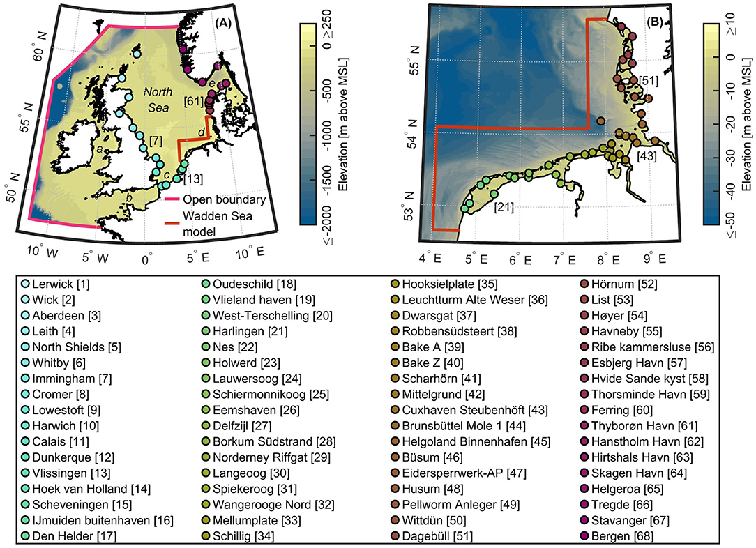
Figure 1. Bathymetric maps for the study area. (A) Bathymetric map for the NWES, including model boundaries and locations of tidal gauges used for model validation. Additional information about the 68 tidal gauges is given in Supplementary Table 1. Letters a to e denote: (a) Irish Sea, (b) English Channel, (c) Southern Bight, (d) German Bight, and (e) Skagerrak. (B) Bathymetric map for the Wadden Sea, including model boundaries and locations of tidal gauges used for model validation.

2.2. Model Set-Up

To investigate the responses of North Sea tidal dynamics to the combined effects of SLR and potential morphological changes in the Wadden Sea, a depth-averaged hydronumerical model based on the software Delft3D was set-up (Lesser et al., 2004). Using a finite difference scheme, Delft3D solves the Reynolds-averaged Navier-Stokes equations on a staggered grid. A detailed description of the used formulations and implementation can be found in Lesser et al. (2004) and Deltares (2020). The model domain extends from 48° N to 62° N in latitudinal direction and from 12° W to around 13° E in longitudinal direction (see Figure 1A). The spatial extent of the domain ensures that the effects of external surges, which can have significant impact on the correct representation of local water levels, are captured in the two-dimensional model. Using spherical coordinates, the grid resolution in latitudinal and longitudinal direction equals 1/50° and 1/32° (≈ 2.3 × 2.3 km), respectively. In order to provide sufficiently fine resolution of local tidal inlets, channels, and intertidal flats, a domain decomposition approach was used to increase the grid resolution in the Wadden Sea to 1/450° and 1/288° (≈ 250 × 250 m) (see red box in Figure 1B). Bathymetric data for the NWES, obtained from the European Marine Observation and Data Network (EMODnet) (EMODnet Bathymetry Consortium, 2018), were complemented by high resolution data for the Dutch, German, and Danish Wadden Sea, originating from the Rijkswaterstaat (Wiegmann et al., 2005), the Bundesanstalt für Wasserbau (BAW) (Sievers et al., 2020a), the Wasserstraßen- und Schifffahrtsverwaltung des Bundes (WSV) (WSV, 2020), and the Kystdirektoratet. The merged and assimilated dataset, with a maximum resolution of 5 × 5 m, was adjusted to MSL as a vertical reference datum and was interpolated onto the numerical grid. Amplitudes and phases for a total of 32 harmonic constituents were extracted from the FES2014 global tide model (Carrère et al., 2016) and taken as model forcing along the open boundary (see pink box in Figure 1A). Furthermore, the model was forced with spatially varying wind (u- and v-component at 10 m height) and pressure fields with a resolution of around 6 × 6 km, originating from the COSMO-REA6 reanalysis dataset (Bollmeyer et al., 2015). Based on the spatially varying pressure fields, an inverse barometer correction was applied. Wind drag coefficients were calculated by using the parameterized model of Wu (1982). Using a wind speed of 30 m/s as an upper limit, a constant wind drag coefficient was assumed above this threshold. To dynamically calculate the bed roughness for each grid cell based on local sediment characteristics, currents, and water depths, the van Rijn (2007) bed roughness predictor was applied. Available data of median grain-sizes (D₅₀) (Rijkswaterstaat, 1998; Bockelmann, 2017; Wilson et al., 2018; Sievers et al., 2020b) were used as input for the bed roughness calculations, in order to incorporate local roughness anomalies.

2.3. Model Validation

The performance of the model was evaluated based on the comparison of simulated and observed water levels for 68 locations across the whole North Sea region (see Supplementary Table 1). Figure 2 shows the agreement between simulated and observed water levels for six selected tidal gauges (see locations in Figure 1) for a full spring-neap cycle (September 28 to October 13, 2012). Concentrating on tidal dynamics, this simulation period only includes moderate wind forcing. The chosen locations reflect the counterclockwise propagation of the tidal wave in the North Sea, entering the basin through its northern boundary with the Atlantic Ocean and propagating along the coasts of the UK, France, Belgium, and the Netherlands, heading eastwards to Germany and finally traveling northbound to Denmark and Norway. A closer examination of the individual time-series of tidal curves reveals that the simulated tidal high and low water levels are corresponding to a high degree with observations acquired in the field. Observed features, including spring and neap tides, diurnal inequalities, and extreme events are also well captured, indicating the model's ability to reproduce the regional hydrodynamics. Furthermore, different statistical parameters were calculated based on the above-mentioned spring-neap cycle to quantify the model skill. A Taylor diagram (Taylor, 2001) was therefore applied, which is based on three statistical measures: i) the standard deviation of the simulation, ii) the Pearson correlation coefficient, and iii) the centered root mean square difference (CRMSD). The Taylor diagram in Figure 3 highlights the modeling quality and individual level of agreement between modeled and observed water levels at the considered locations. For each gauge station, the simulated standard deviation and CRMSD were normalized by dividing these quantities by the standard deviation of the observation. A perfect model fit has a normalized standard deviation of 1, a correlation coefficient of 1 and a normalized CRMSD of 0. Deviations between model results and observations are largest along the Danish and Norwegian coasts, where tidal ranges are small in the close vicinity of amphidromic points. Accordingly, even differences of just a few centimeters affect the model's fit at these locations significantly. However, the overall agreement between model results and observations is confirmed by averaging the quantities of the Taylor diagram across all locations. The mean normalized standard deviation nearly shows an ideal value (1.03), while the mean correlation coefficient is high (0.9826) and the mean normalized CRMSD is rather small (0.18).

FIGURE 2

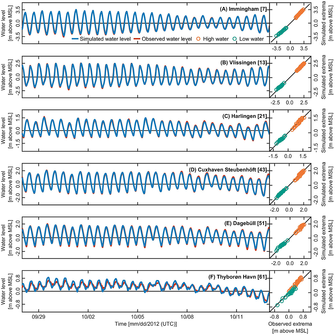
Figure 2. Agreement between simulated and observed water levels at selected tidal gauge stations, according to the spring-neap cycle from September 28 to October 13, 2012. Comparison of simulated and observed water levels at the tidal gauge stations of (A) Immingham, (B) Vlissingen, (C) Harlingen, (D) Cuxhaven-Steubenhöft, (E) Dagebüll, and (F) Thyborøn Havn. Locations of tidal gauges are shown in Figure 1.

FIGURE 3

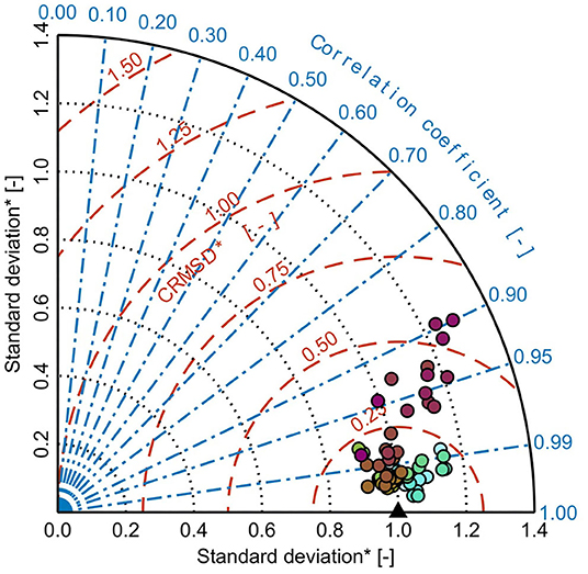
Figure 3. Model performance according to the Taylor diagram, using the standard deviations, Pearson correlation coefficients, and CRMSDs. The spring-neap cycle from September 28 to October 13, 2012, was used for the calculation of statistical parameters. Quantities that were normalized by the standard deviations of the observational data are indicated by *. The black triangle indicates a perfect model fit. The color codes and locations of tidal gauges are shown in Figure 1.

Furthermore, a harmonic analysis was performed to compare observed and simulated amplitudes of selected tidal constituents. For this analysis, a simulation period of 3 months was set (September 1 to December 1, 2012), since this period is sufficient to determine the amplitudes of the most relevant tidal constituents in the North Sea (Rasquin et al., 2020). The T_TIDE toolbox was applied to perform the harmonic analysis of tidal water levels. Further details regarding the principle of classical tidal harmonic analysis and the underlying formulations of T_Tide can be found in Pawlowicz et al. (2002). Figure 4 shows the agreement for the main tidal constituents M2 and O1, the higher harmonic M4, and the frictional tide M6. Generally, the model results show no inherent over- or underestimation of magnitudes of tidal constituents and are in good agreement with observational data. Only at a few locations, the results for the higher harmonic M4 and the frictional tide M6 show mismatches between simulated and observed data. Across all locations, the root mean square error (RMSE) values for the dominant constituent M2 and its higher harmonic M4 are 7.3 and 2.5 cm, respectively. The RMSE values for the constituents O1 and M6 are ≤ 1 cm. Owed to the thorough validation, based on a high number of reference gauges, the quality of our model is similar or even superior to previous shelf models (e.g., Pickering et al., 2012; Ward et al., 2012; Arns et al., 2015), indicating the ability to reproduce the regional hydrodynamic processes to a more than satisfying degree. Thus, it is also reasonable to conclude that the model set-up and its performance for the validation period are trustworthy to conduct further investigations regarding plausible scenarios of SLR and morphological changes in the Wadden Sea.

FIGURE 4

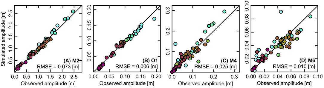
Figure 4. Agreement of tidal constituents calculated by harmonic analysis of observed and simulated water levels, according to the 3-month period from September 1 to December 1, 2012. Comparison of observed and simulated amplitudes for the tidal constituents (A) M2, (B) O1, (C) M4, and (D) M6. The color codes and locations of tidal gauges are shown in Figure 1.

2.4. Scenario Development

Based on the results of the validation, the model was used to assess the responses of the regional tides to plausible future scenarios, which were developed in this study. Besides the present-day baseline scenario, simulations with 0.8 and 2.0 m SLR were run by adding these values to the bathymetry. A global mean SLR of 0.8 m by the end of this century is in accordance with the latest findings on SLR, following the RCP8.5 emission scenario (Oppenheimer et al., 2019). A SLR of 2.0 m represents a high-end projection (Kopp et al., 2017; Wong et al., 2017) that is certainly beyond recent expectations, but could easily be reached by the year 2100 or beyond if today's mitigation efforts to reduce greenhouse gas emissions fail. This high-end projection has also been assessed in numerous previous studies of future North Sea tidal dynamics (Pickering et al., 2012; Ward et al., 2012; Pelling et al., 2013), hence enabling a direct comparison of results between different modeling attempts. In order to assess the model's sensitivity to accompanying morphological changes in the Wadden Sea, different cumulative rates of vertical accretion were applied to the local intertidal areas. Thus, the model addresses the questions how and to which degree local intertidal areas will contribute to future changes in North Sea tidal dynamics. Generally, if SLR is below a critical limit, a dynamic equilibrium is established and intertidal areas are able to keep up with SLR (Van Goor et al., 2003; Dissanayake et al., 2012; Lodder et al., 2019). This critical limit can vary substantially between tidal basins in close proximity to one another (Van Goor et al., 2003; Lodder et al., 2019). By analyzing digital elevation models (DEMs) of intertidal flats in the Wadden Sea, a recent study finds evidence that the accumulation of marine aggregates presently compensates observed SLR (Benninghoff and Winter, 2019). However, numerical studies (Dissanayake et al., 2012; Becherer et al., 2018) indicate that future vertical accretion in the local intertidal flats is insufficient to compensate for projected SLR by the year 2100. Depending on the future magnitude and acceleration of SLR in the coming decades, intertidal flat systems in the Wadden Sea could be significantly diminished or may even disappear completely (Dissanayake et al., 2012). Considering these uncertainties, different cumulative rates of vertical accretion were used, ranging from 0 to 100% of projected SLR, thus mimicking variation of local water depths in shallow water environments. For the case of no vertical accretion (0%), a significant sediment deficit is assumed and intertidal flats are incapable to rise with the sea-level, which might be the case if a rapid, accelerated SLR is experienced (e.g., Dangendorf et al., 2017). For 100% vertical accretion, it is assumed that sediment input can counterbalance projected levels of SLR and intertidal flats are able to keep up with SLR. The other considered rates of vertical accretion (25%, 50%, 75%) assume that the local sediment availability leads to moderate accretion in the intertidal flats, which can partly balance the effects of SLR. Including the baseline scenario, combinations of the different SLR projections and the various rates of vertical accretion led to a total of 11 scenarios. These scenarios, which are summarized in Table 1, reflect a multitude of reasonable and sound future developments of drivers and parameters that may impact the future responses of the regional tides. Figure 5 shows the changes in local water depths in the Wadden Sea, which are associated with a SLR of 0.8 m and the various rates of vertical accretion. Changes in water depths for a SLR of 2.0 m and the various rates of vertical accretion can be found in Supplementary Figure 1. Additionally, exemplary hypsometric curves for the Elbe estuary, which also reflect changes in water depths associated with the outlined scenarios, are given in Supplementary Figure 2.

TABLE 1

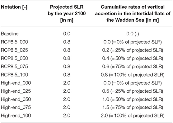
Table 1. Notations of investigated scenarios as well as associated values of SLR and cumulative rates of vertical accretion.

FIGURE 5

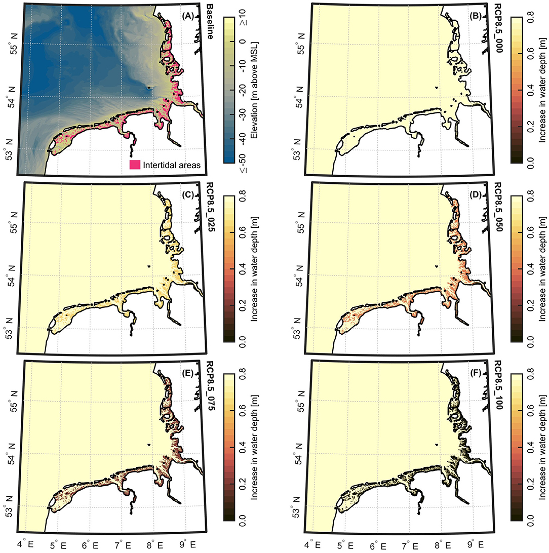
Figure 5. Combinations of 0.8 m SLR projection and various cumulative rates of vertical accretion in the Wadden Sea. (A) Bathymetric map for the Wadden Sea, including locations of intertidal flats. Local increases in water depths for scenarios (B) RCP8.5_000, (C) RCP8.5_025, (D) RCP8.5_050, (E) RCP8.5_075, and (F) RCP8.5_100.

Even though our modeling approach uses highly resolved bathymetric data in the intertidal flats of the Wadden Sea, thus compensating for shortcomings of previous numerical studies of North Sea tidal dynamics, several assumptions and simplifications are inherent to our scenario simulations. As proposed by Pickering et al. (2012), the model's open boundary was implemented in deep water and far away from the shelf. Accordingly, it can be assumed that the effects of SLR on the tidal forcing along this boundary are insignificant. Furthermore, no river discharges were applied to the upstream boundaries of the Ems, Weser, and Elbe estuaries, even though they are included in the model. It is, however, proven that the exclusion of the local hydrology in the adjacent estuaries only has minimal impact on the regional tidal dynamics of the German Bight, as discussed and shown by Rasquin et al. (2020). Regarding the future morphological evolution of intertidal areas in the Wadden Sea, the availability of sediments from internal and external sources has to be considered. Tidal inlets, channels, and ebb-tidal deltas act as internal sediment sources in a tidal basin, while external sediments may be provided by foreshore areas, barrier islands, or remote sites (Wachler et al., 2020). Existing empirical (Hofstede, 2002) and schematized models (Van Goor et al., 2003) have shown that SLR may cause an internal sediment redistribution from tidal inlets, channels, and ebb-tidal deltas to the intertidal flats. As a result, vertical accretion in the intertidal flats is usually associated with a simultaneous erosion in the inlets and channels, as recently observed by Benninghoff and Winter (2019). We assumed that sediments from external sources are fully accountable for the vertical accretion in the intertidal flats of the Wadden Sea for simplicity. In contrast to Wachler et al. (2020), a deepening of local tidal inlets and channels was neglected in our model. Furthermore, we uniformly applied each considered rate of vertical accretion to the entire intertidal flats of the Wadden Sea. Even though the morphological responses of individual tidal basins to SLR may vary substantially (Van Goor et al., 2003; Lodder et al., 2019), spatially varying patterns of vertical accretion were deemed unfeasible for the original focus in our study. Finally, we assumed that predominant sediment grain-sizes, which were used as input in the bed roughness calculations, remain stable despite rising sea-levels. The effects of SLR and altered hydrodynamics on the amount of fine-grained sediments in intertidal flats (Dolch and Hass, 2008) were accordingly also neglected. Focusing on the general responses of North Sea tides to SLR and morphological changes in the intertidal flats of the Wadden Sea, these mentioned assumptions and simplifications were considered acceptable.

3. Results

To analyze the responses of the North Sea tides to SLR and morphological changes in the Wadden Sea, the assessment considers the likely alterations in the amplitudes of the dominant semi-diurnal tidal constituent M2. Due to the application of harmonic analysis, the impact of the wind forcing can be neglected in our results. In detail, we analyzed spatial patterns of M2 amplitude increases and decreases. Observed changes in M2 amplitudes are strongly linked to the forced migration of amphidromic points. Accordingly, their movements in response to the different scenarios are also presented, while mainly focusing on the amphidromic point in the German Bight. Changes in the shape of tidal curves and associated alterations in tidal asymmetry (i.e., flood and ebb dominance) in prominent adjacent estuaries are also discussed. Results for 0.8 m SLR and the various rates of vertical accretion are presented first, followed by the analysis of scenarios, which are associated with a SLR of 2.0 m. In addition, the comparison of the tidal responses to 0.8 and 2.0 m SLR enables the assessment of the non-linearity of amplitude changes.

3.1. Responses of Regional Tides to 0.8 m SLR

Figure 6 shows the alterations in M2 amplitudes across the NWES for a SLR of 0.8 m and the various rates of vertical accretion in the intertidal flats of the Wadden Sea. Except for the Wadden Sea, spatial patterns of amplitude increases and decreases remain relatively stable for most of the North Sea region, only varying in the magnitude of amplitude changes (see Figures 6B–F). Regions of significant amplitude increases are located at the British coast between Aberdeen and Whitby, the bulk of the Southern Bight, and the Skagerrak. Regions of amplitude decreases are seen northwards of Aberdeen, between Immingham and Cromer, in the northeastern part of the Southern Bight, and along the west coast of Norway. Other areas of particular M2 amplitude increases (e.g., northern half of Irish Sea, eastern half of English Channel) and decreases (e.g., southernmost Irish Sea, western half of English Channel), which lie outside the North Sea region, are not in the focus of our study. It also must be noted that M2 amplitude changes for presented scenarios are insignificant along the open boundary (<1 cm), as previously assumed.

FIGURE 6

Figure 6. M2 amplitudes for the NWES resulting from the combinations of 0.8 m SLR projection and various cumulative rates of vertical accretion. (A) Map of M2 amplitudes for the NWES for the baseline scenario, according to the 3-month period from September 1 to December 1, 2012. Relative changes in M2 amplitudes for scenarios (B) RCP8.5_000, (C) RCP8.5_025, (D) RCP8.5_050, (E) RCP8.5_075, and (F) RCP8.5_100.

In contrast to the remainder of the domain, the M2 amplitude responses are distinctly different between the investigated scenarios for the Wadden Sea area. For increased near-shore water depths, following the scenario of no vertical accretion in the intertidal flats (RCP8.5_000) (see Figure 6B), significant decreases in M2 amplitudes are observed in the German Bight and along the adjacent Danish coast. With increasing vertical accretion in the intertidal flats of the Wadden Sea (RCP8.5_025 to SLR0.8_075), areas with amplitude increases are extending, while areas with M2 amplitude decreases begin to diminish (see Figures 6C–E). In the case of 100% vertical accretion (RCP8.5_100), substantial amplitude increases are noticed along the entire Wadden Sea coast (see Figure 6F). Due to the sensitivity of the region to the different scenarios, M2 amplitude alterations in the Wadden Sea are shown in more detail in Figure 7. Since intertidal flats are more frequently or even permanently inundated for a SLR of 0.8 m, they show the most pronounced increases in M2 amplitudes. In the case of no vertical accretion (RCP8.5_000), the amphidromic point in the German Bight shifts in northeast direction by around 7 km, thus moving closer toward the coast of Denmark (see Figure 7B). With increasing vertical accretion in the Wadden Sea, this amphidromic point migrates back in the direction of its present-day location (see Figures 7C–F). The closer the amphidromic point shifts toward its present location, the more areas become subject to increases in M2 amplitudes. The magnitudes of M2 amplitudes are also visibly affected, indicating that the shift of this amphidromic point has significant impact on the overall tidal responses in the Wadden Sea. Plausible physical drivers and inherent mechanisms forcing the migration of this amphidromic point are discussed in detail in section 4. Other amphidromic points in the North Sea region (e.g., in the Southern Bight) however show no sensitivity toward the different rates of vertical accretion in the Wadden Sea and thus are not presented here.

FIGURE 7

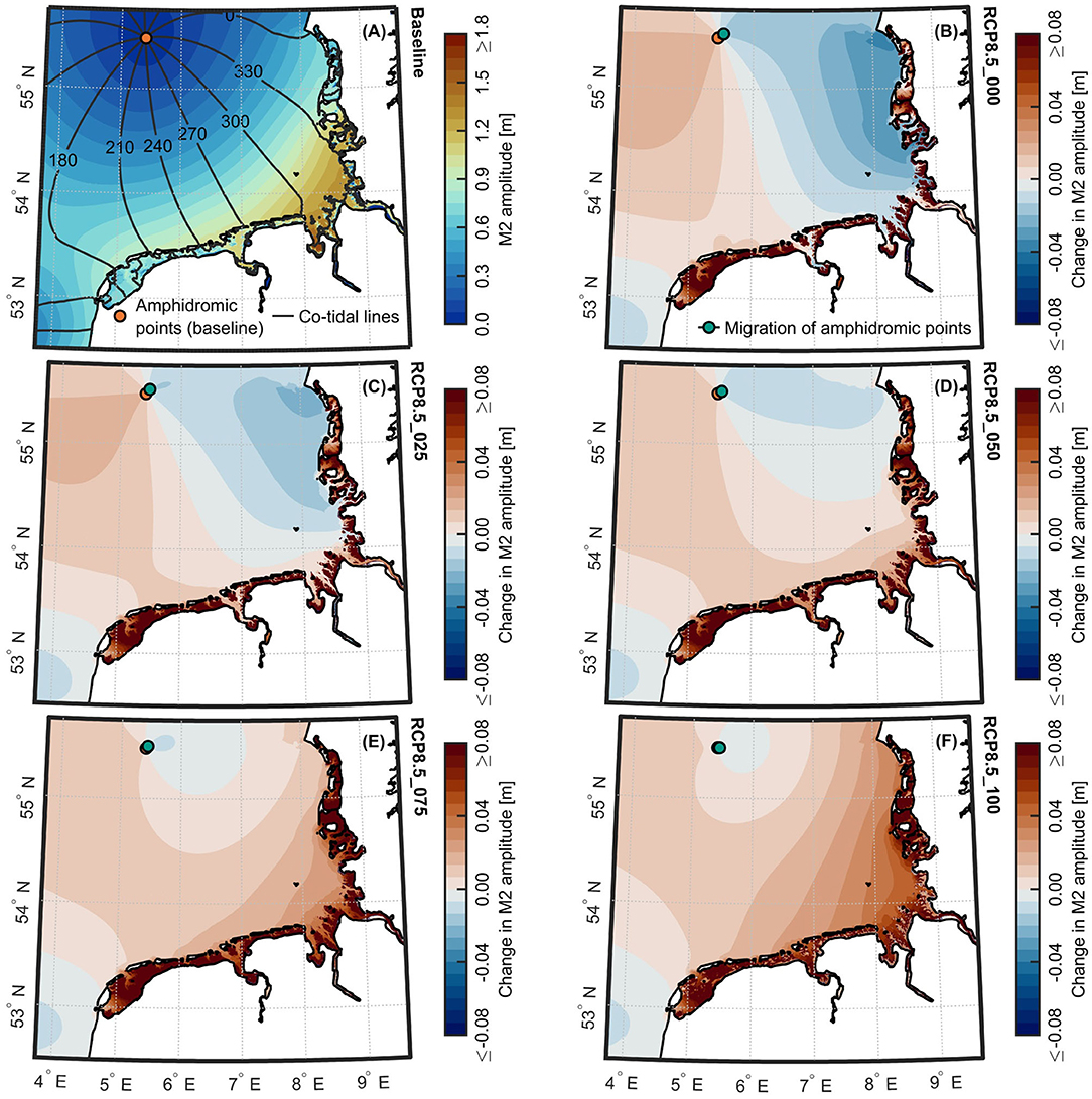
Figure 7. M2 amplitudes for the Wadden Sea resulting from the combinations of 0.8 m SLR projection and various cumulative rates of vertical accretion. (A) Map of M2 amplitudes for the Wadden Sea for the baseline scenario, according to the 3-month period from September 1 to December 1, 2012. Relative changes in M2 amplitudes for scenarios (B) RCP8.5_000, (C) RCP8.5_025, (D) RCP8.5_050, (E) RCP8.5_075, and (F) RCP8.5_100. Green dots indicate movements of amphidromic points in relation to the baseline scenario (orange dots).

To quantify the tidal responses of the North Sea basin to our scenarios, Figure 8 shows the M2 amplitude changes for the 68 tidal gauge locations, which were previously used for the validation of the model. For each site, Figure 8B highlights the range of possible alterations in the responses of the M2 tide, which are associated with a SLR of 0.8 m and the various cumulative rates of vertical accretion. The three largest decreases in M2 amplitudes occur at the locations Pellworm Anleger (−3 cm), Husum (−3 cm), and Büsum (−3 cm) for scenario RCP8.5_000. The three largest absolute increases occur at the locations Dagebüll (+13 cm), Harlingen (+12 cm), and Delfzijl (+12 cm), assuming that the vertical accretion in the intertidal flats is able to keep up with a SLR of 0.8 m (RCP8.5_100). Following the propagation of the tidal wave, M2 amplitude changes between the morphological scenarios are almost negligible from Lerwick to Den Helder, which marks the southwest edge of the Wadden Sea. Along the coasts of the Wadden Sea, significant differences prevail between the scenarios. Between scenarios RCP8.5_000 and RCP8.5_100, the differences in M2 amplitudes even surpass 10 cm at multiple locations. The largest differences are observed at the locations Dagebüll (−1 cm for RCP8.5_000, +13 cm for RCP8.5_100), Husum (−3 cm for RCP8.5_000, +9 cm for RCP8.5_100), and Pellworm Anleger (−3 cm for RCP8.5_000, +8 cm for RCP8.5_100). This highlights that the North Frisian coastal region of the Wadden Sea is particularly sensitive to the combined effects of a SLR of 0.8 m and the various cumulative rates of vertical accretion. However, even a remote region like the Skagerrak, which is located hundreds of kilometers away from the Wadden Sea, also shows a significant sensitivity toward the applied morphological changes. Plausible implications for the Baltic Sea (e.g., inflow of saline water, stratification, nutrient influx) are not addressed in this study.

FIGURE 8

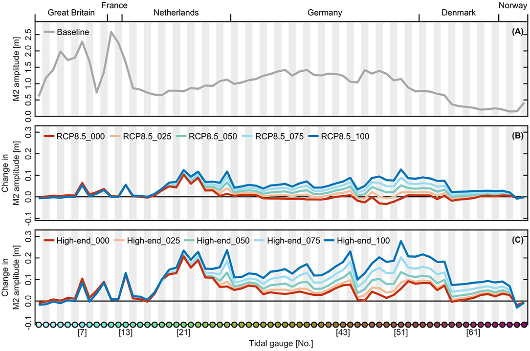
Figure 8. M2 amplitudes as a function of available tidal gauge stations resulting from the combinations of different SLR projections and various cumulative rates of vertical accretion. (A) M2 amplitudes for the baseline scenario, according to the 3-month period from September 1 to December 1, 2012. (B) Relative changes in M2 amplitudes resulting from 0.8 m SLR and various cumulative rates of vertical accretion. (C) Relative changes in M2 amplitudes resulting from 2.0 m SLR and various cumulative rates of vertical accretion. The color codes and locations of tidal gauge stations are shown in Figure 1. Shown numbers indicate exemplary tidal gauge stations that were highlighted in more detail in Figure 2.

The tidal curves for the tidal gauge stations, which were previously shown in Figure 2, reveal some interesting features (see Figure 9). With very few exceptions (e.g., Dagebüll in the case of scenario RCP8.5_000), tidal high water levels tend to rise for a SLR of 0.8 m, while tidal low water levels concurrently fall. As a result, the tidal ranges (and M2 amplitudes) are likely to increase. Figure 9 also shows that a phase shift of the M2 constituent occurs for a SLR of 0.8 m, as indicated by an earlier occurrence of the tidal high and low water levels. This is explained by an increase in the propagation speed of the tidal wave with increasing sea-level and larger water depths inside the North Sea basin. The stations of Immingham (Figure 9A) and Vlissingen (Figure 9B), though, show no sensitivity toward the vertical accretion in the Wadden Sea. In contrast, the stations Harlingen, Cuxhaven-Steubenhöft, Dagebüll, and Thyborøn Havn (see Figures 9C–F) show substantially different responses between the scenarios. At these locations, magnitudes of changes in tidal high and low water levels become more pronounced with increasing vertical accretion in the intertidal areas of the Wadden Sea. For the stations of Harlingen and Dagebüll it is also shown that alterations in tidal low water levels are larger in relation to the tidal high water levels. In addition, it becomes apparent that the morphological evolution of the Wadden Sea not only affects local high and low water levels in the case of a SLR, but also influences the shape of the tidal wave, as seen in Figures 9C–F. For all available gauge locations, detailed changes in tidal high and low water levels are presented in the Supplementary Figures 3, 4, respectively.

FIGURE 9

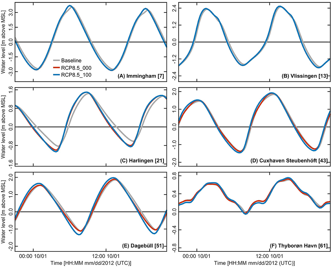
Figure 9. Distortion of the tidal wave at selected tidal gauge stations resulting from combinations of 0.8 m SLR projection and various cumulative rates of vertical accretion. Distortion of the tidal wave at the tidal gauge stations of (A) Immingham, (B) Vlissingen, (C) Harlingen, (D) Cuxhaven-Steubenhöft, (E) Dagebüll, and (F) Thyborøn Havn. Comparisons are based on an exemplary 25 hour period during spring tide (boundary forcing equals conditions for September 30 to October 1, 2012). Locations of tidal gauges are shown in Figure 1.

An altered distortion and more pronounced asymmetry of the tidal wave, as shown in Figure 9, supposedly has strong implications for the sediment transport in the estuaries of the German rivers Ems, Weser, and Elbe. Thus, we also briefly assessed the tidal duration asymmetry by analyzing phase differences between the M2 and M4 tidal constituents. By means of the widely applied definition by Friedrichs and Aubrey (1988), positive values for the indicator sin(2Θ_M2−Θ_M4) denote an estuarine system showing flood dominance, while negative values are typically associated with ebb dominance. Here, Θ_M2 and Θ_M4 are the sea-surface phases of the M2 and M4 tidal constituents. In the case of a symmetric tide, sin(2Θ_M2−Θ_M4) is equal to zero. In this context, flood dominance is associated with a shorter flood than ebb duration and stronger peak flood currents, resulting in a net import of sediments into an estuary. Conversely, ebb dominance results in shorter ebb duration than flood duration, stronger peak ebb currents, and a flushing of sediments in seaward direction. According to this definition, the Ems, Weser, and Elbe estuaries already show flood dominance under present-day conditions (see Figure 10A). In this context, it must be noted that the influence of freshwater discharges was neglected in our simulations. In the case of a SLR of 0.8 m and no vertical accretion in the Wadden Sea (RCP8.5_000), the loss of intertidal storage volume leads to an increase in flood dominance (or a decrease in ebb dominance) in the respective estuaries (see Figure 10B). The more intertidal storage volume becomes available due to vertical accretion in the Wadden Sea, the more the tendencies for flood and ebb dominance resemble the present-day state (see Figures 10C–F).

FIGURE 10

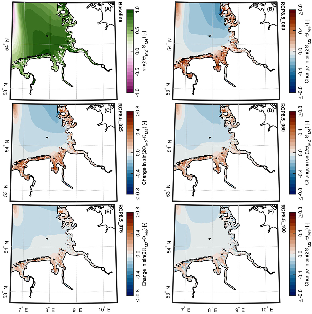
Figure 10. Flood and ebb dominance for the German Bight resulting from the combinations of 0.8 m SLR projection and various cumulative rates of vertical accretion. (A) Map of flood and ebb dominance for the German Bight for the baseline scenario, according to the 3-month period from September 1 to December 1, 2012. Relative changes in flood and ebb dominance for scenarios (B) RCP8.5_000, (C) RCP8.5_025, (D) RCP8.5_050, (E) RCP8.5_075, and (F) RCP8.5_100. In panel (A), values > 0 indicate flood dominance, with values <0 signaling ebb dominance. In panels (B) to (F), values > 0 indicate increases in flood dominance or decreases in ebb dominance, while values <0 signal increased ebb dominance or decreased flood dominance.

3.2. Responses of Regional Tides to 2.0 m SLR

The M2 amplitude alterations for a SLR of 2.0 m and the various cumulative rates of vertical accretion are shown in Figure 11. In comparison to a SLR of 0.8 m, as portrayed in Figure 6, the limits of the color bars were adjusted in proportion to the increased SLR. Compared to a SLR of 0.8 m, the M2 amplitude changes are amplified, while the associated spatial patterns of amplitude increases and decreases show only minor alterations. Again, regions of amplitude increases are foremost found between Aberdeen and Whitby, in the central part of the Southern Bight, and the Skagerrak. Regions of amplitude decreases are located in the north of Scotland, near the Wash estuary, in the northernmost part of the Southern Bight, and along the Norwegian west coast.

FIGURE 11

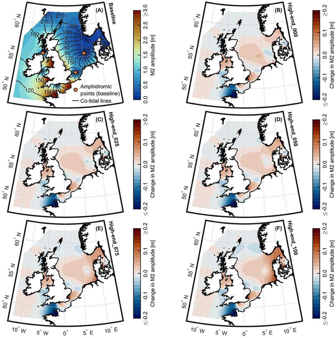
Figure 11. M2 amplitudes for the NWES resulting from the combinations of 2.0 m SLR projection and various cumulative rates of vertical accretion. (A) Map of M2 amplitudes for the NWES for the baseline scenario, according to the 3-month period from September 1 to December 1, 2012. Relative changes in M2 amplitudes for scenarios (B) high-end_000, (C) high-end_025, (D) high-end_050, (E) high-end_075, and (F) high-end_100.

For a SLR of 2.0 m, the responses of the tidal signal in the Wadden Sea can be quite different between the various rates of vertical accretion (see Figures 11, 12). As previously depicted for a SLR of 0.8 m, the amphidromic point in the German Bight migrates the furthest in northeast direction (≈ 12 km) in the case of no vertical accretion (high-end_000) (see Figure 12B). With increasing vertical accretion, this amphidromic point moves back in the opposite direction toward its present location (see Figures 12C–F). In contrast to a SLR of 0.8 m, only the North Frisian Wadden Sea and a smaller section of the adjacent Danish coast are subject to decreases in M2 amplitudes if no vertical accretion is assumed (high-end_000). Independent from the rate of vertical accretion, the remainder of the Wadden Sea exhibits increases in M2 amplitudes for a SLR of 2.0 m. The higher the vertical accretion, the more the M2 amplitudes are amplified in those regions. The North Frisian and Danish coasts become subject to increases in M2 amplitudes, too, with increasing vertical accretion in the local intertidal flats. In relation to a SLR of 0.8 m, the observed alterations in the patterns of M2 amplitude increases and decreases also reveal non-linear behavior in response to SLR.

FIGURE 12

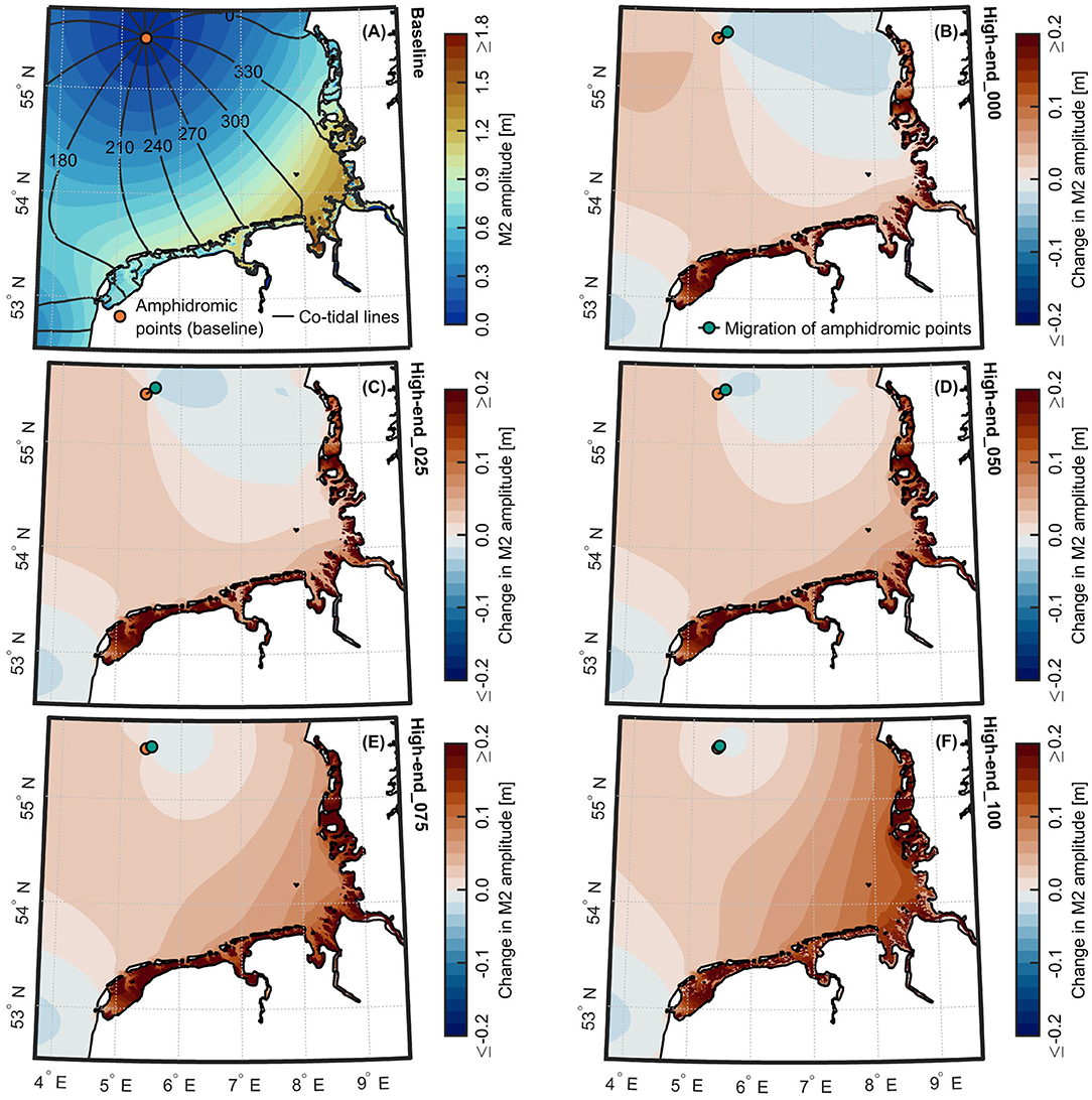
Figure 12. M2 amplitudes for the Wadden Sea resulting from the combinations of 2.0 m SLR projection and various cumulative rates of vertical accretion. (A) Map of M2 amplitudes for the Wadden Sea for the baseline scenario, according to the 3-month period from September 1 to December 1, 2012. Relative changes in M2 amplitudes for scenarios (B) high-end_000, (C) high-end_025, (D) high-end_050, (E) high-end_075, and (F) high-end_100. Green dots indicate movements of amphidromic points in relation to the baseline scenario (orange dots).

Detailed alterations in the M2 amplitudes resulting from a SLR of 2.0 m and the various cumulative rates of vertical accretion are shown in Figure 8C for a total of 68 tidal gauges across the entire North Sea region. The three largest decreases in M2 amplitudes occur at Stavanger (−3 cm), Lerwick (−2 cm), and Wick (−2 cm) in the case of scenario high-end_100. The three largest absolute amplitude increases, which are observed at the locations Dagebüll (+28 cm), Delfzijl (+24 cm), and Harlingen (+23 cm), are also associated with scenario high-end_100. Between the investigated scenarios, the differences in M2 amplitudes are again substantial along the coasts of the Wadden Sea and the northward located part of the Danish coast. Maximum differences between scenarios high-end_000 and high-end_100 are as high as 22 cm. The largest differences occur at Dagebüll (+6 cm for high-end_000, +28 cm for high-end_100), Husum (+3 cm for high-end_000, +20 cm for high-end_100), and Delfzijl (+7 cm for high-end_000, +24 cm for high-end_100).

In comparison to a SLR of 0.8 m, changes in individual tidal curves (e.g., magnitudes of tidal high and low water levels, phase shifts) become more pronounced for a SLR of 2.0 m (see Supplementary Figure 5). Largest changes are to be expected if intertidal areas are capable to import an adequate amount of sediments to fully rise with the sea-level (high-end_100). Associated changes in tidal asymmetries (i.e., magnitudes of flood and ebb dominance) are also enhanced for a SLR of 2.0 m (see Supplementary Figure 6). As previously observed for a SLR of 0.8 m, the largest increases in flood dominance (and decreases in ebb dominance) occur in the case of no vertical accretion in the Wadden Sea (high-end_000).

4. Discussion

4.1. Mechanisms for Observed Changes

Taylor (1922) investigated the reflection of Kelvin waves for a semi-enclosed, rotating basin of uniform width and depth. For this problem, the superposition of Kelvin waves (incoming and reflected) and generated Poincaré waves leads to the formation of an amphidromic system, with the amphidromic points being aligned along the centerline of the basin. Hendershott and Speranza (1971) introduced a dissipative boundary condition to Taylor's solution, while Rienecker and Teubner (1980) added the effect of bottom friction. Both incorporated effects lead to a shift of amphidromic points in cross-basin direction, even though the displacements of amphidromic points are different. Based on these idealized solutions, M2 amplitude changes can generally be explained by different spatial patterns of energy dissipation, which lead to varying migrations of amphidromic points in return. To shed more light on the responses of the North Sea tides to the scenarios discussed above, the energy dissipation was therefore calculated for each scenario. To estimate the energy dissipation, the standard expression for tidal boundary layers, which assumes a balance between bottom stress and energy dissipation, was used:

$\begin{array}{ll}ϵ=\rho ·C_d·\left|u\right|{}^{\text{3}}& (1)\end{array}$

where ρ is the water density (ρ = 1,025 kg/m³), C_d is the bed friction coefficient and u is the tidal velocity vector. Concentrating on the Wadden Sea area (see red box in Figure 1B), the mean tidal energy dissipation for the baseline scenario amounts to around 6,300 MW, based on an exemplary spring-neap cycle (September 28 to October 13, 2012). In relation to the baseline, the energy dissipation for the different scenarios increases between around +2 and +7% for a SLR of 0.8 m. The lower the vertical accretion in the Wadden Sea, the higher the increase in energy dissipation becomes. Accordingly, the highest energy dissipation is associated with scenario RCP8.5_000, while scenario RCP8.5_100 shows the smallest increase in tidal energy dissipation. As expected, the displacement of the amphidromic point in the German Bight becomes larger, the more energy dissipation occurs (see Figures 7B–F). For a SLR of 2.0 m and the various rates of vertical accretion, the energy dissipation increases between around +4 and +13% in comparison to the baseline. Thus, movements of the amphidromic point in the German Bight are more pronounced for a SLR of 2.0 m. Again, the largest increase in energy dissipation occurs for 0% vertical accretion (high-end_000), while the smallest increase occurs for 100% vertical accretion (high-end_100). The detailed rates of energy dissipation for our scenarios are shown in Supplementary Table 2.

Caused by different rates of energy dissipation, the observed migrations of the amphidromic point in the German Bight and subsequent M2 amplitude changes can be explained adequately. It is still uncertain though, which mechanisms are responsible for the presented increases in tidal energy dissipation. The investigation of different coastal defense strategies by Pelling et al. (2013) showed that the flooding of additional grid cells within a numerical model can be an important mechanism controlling the responses of North Sea tidal dynamics to SLR. For a fixed coastline, the energy dissipation decreased across their whole model domain with increasing SLR. In contrast, present-day dissipation rates were maintained for a coastal recession scenario. New areas of high energy dissipation were created by the flooding of the low-lying Dutch coast, counterbalancing the effects of decreasing energy dissipation with increasing water depths. However, we assumed that coastal protection measures will be in place and even re-strengthened in order to cope with SLR and protect the present-day coastline, thus following a fixed and fortified coastal protection strategy. In relation to the baseline, no additional cells are available for flooding in any of our outlined future scenarios. Accordingly, the flooding of new cells cannot be the controlling mechanism that leads to the different responses in M2 amplitudes. In addition, as shown by Rasquin et al. (2020), intertidal flats in the Wadden Sea, which will be inundated more frequently or even permanently due to SLR, contribute only marginally to the local energy dissipation.

Observed differences in the rates of energy dissipation can likely be explained by alterations in the mean current velocities, as suggested by Rasquin et al. (2020). For a SLR of 0.8 m, the alterations in mean current velocities due to the various rates of vertical accretion are shown in Figure 13. As described by Wachler et al. (2020), changes in the velocity patterns due to SLR are mainly controlled by the ratio of tidal prism to cross-sectional area of local tidal inlets and channels. For no vertical accretion, they showed that this ratio increases with rising sea-levels. As a result, the mean velocity magnitudes in the tidal inlets and channels will be increased, which can also be observed in our results, as seen Figure 13B. For a SLR of 0.8 m, with simultaneous vertical accretion of tidal flats by 0.5 m and a deepening of tidal channels by 0.2 m, Wachler et al. (2020) also showed that this ratio decreases again. With regard to the tidal velocities, the system's responses to SLR were counterbalanced by the applied bathymetric changes. As can be deduced from Figures 13C–F, these effects are also evident in our results. In most of the tidal inlets and channels, the mean velocity magnitudes will decrease with increasing vertical accretion in the local intertidal flats. It seems reasonable that the observed alterations in M2 amplitudes are caused by these changes in mean current velocities, since current velocities are strongly linked to the energy dissipation. The changes in mean current velocities for a SLR of 2.0 m and the various cumulative rates of vertical accretion can be found in Supplementary Figure 7.

FIGURE 13

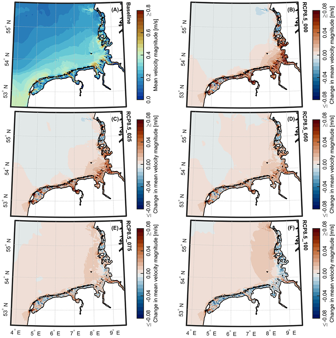
Figure 13. Mean velocity magnitudes for the Wadden Sea resulting from the combinations of 0.8 m SLR projection and various cumulative rates of vertical accretion. (A) Map of mean velocity magnitudes for the Wadden Sea for the baseline scenario, according to the spring-neap cycle from September 28 to October 13, 2012. Relative changes in mean velocity magnitudes for scenarios (B) RCP8.5_000, (C) RCP8.5_025, (D) RCP8.5_050, (E) RCP8.5_075, and (F) RCP8.5_100.

At this point, we also want to briefly discuss the possible impact of our simplifications and assumptions on the results. For simplicity, we assumed that sediments from external sources are fully accountable for the vertical accretion in the intertidal areas of the Wadden Sea. However, it is likely that a redistribution of sediments from tidal inlets and channels to the intertidal areas will partially contribute to the vertical accretion. If tidal inlets and channels are deepened, the ratio of tidal prism to cross-sectional area will decrease. As discussed in detail by Wachler et al. (2020), this further decreases current velocities in the inlets and channels in comparison to a SLR without considering potential bathymetric changes in the Wadden Sea. Due to the interconnections between tidal velocities, energy dissipation rates, and tidal amplitudes, we conclude that the differences in M2 amplitudes between scenarios could even be higher than presented here if future erosion in the inlets and channels is assumed. Furthermore, we applied considered rates of vertical accretion uniformly to the entire intertidal areas of the Wadden Sea. Due to given uncertainties in the response of individual tidal basins to SLR, it was simply unfeasible to use spatially varying rates of vertical accretion in our study. Accordingly, it should be noted that future changes in current velocities and M2 amplitudes could exhibit more complex spatial patterns than shown in our study. Finally, we also assumed that sediment properties (e.g., D₅₀) will remain constant. Variations in sediment properties would impact the bed roughness, which is linked to the bed shear stress. As a result, changes in bed shear stress would also trigger feedbacks on the current velocities, energy dissipation rates and ultimately the amplitudes of tidal constituents. Even though simplifications and assumptions were needed to address future uncertainties, they are common practice in numerical modeling studies. Thus, we are confident that our results give a reliable estimate regarding the future response of regional tidal dynamics to SLR and morphological changes in the Wadden Sea.

4.2. Comparison to Previous Studies

For the North Sea region, the responses of the M2 tide to a SLR of 2.0 m were recently further investigated in numerous studies (Pickering et al., 2012; Ward et al., 2012; Pelling et al., 2013). None of these studies, however, considered the effects of morphological changes on the regional tides. Accordingly, a comparison of results is only feasible for our scenario high-end_000. Our spatial pattern of M2 amplitude increases and decreases is consistent with the results of Pickering et al. (2012) throughout most of the North Sea. Discrepancies are only apparent in the Wadden Sea: Whereas the findings by Pickering et al. (2012) show significant increases in M2 amplitudes along the entire Dutch, German, and Danish coasts, our results indicate decreases in M2 amplitudes in the North Frisian Wadden Sea and along the adjacent Danish coast. The study by Ward et al. (2012) found significant decreases in M2 amplitudes extending from the Netherlands to the Skagerrak. In contrast to Pickering et al. (2012) and our results, they postulated a coastal recession strategy, thus allowing the flooding of extended areas in the Dutch hinterland, which is in stark contrast to present-day coastal protection strategies (Haasnoot et al., 2020). Applying a fixed coastline approach and using the same model as Ward et al. (2012), the pattern of M2 amplitude changes found by Pelling et al. (2013) exhibits strong similarities to our findings. However, as pointed out by Rasquin et al. (2020), the above-mentioned models used relatively coarse resolution (≥ 8 km) throughout their entire model domains. These models are thus not able to represent characteristic bathymetric features in the Wadden Sea, like tidal inlets, channels, and intertidal flats correctly. Considering alterations in local current velocities, which play an important role in the responses of regional tidal dynamics to SLR, the results of these models are sound but imprecise. Taking this shortcoming into consideration, we used a fine grid resolution of around 250 x 250 m in the entire Wadden Sea, thus ensuring a more adequate representation of local shallow water environments.

Furthermore, a recent study by Rasquin et al. (2020) investigated the responses of tidal dynamics in the German Bight to a SLR of 0.8 m, neglecting vertical accretion in the local intertidal flats. Accordingly, their results must be related to our scenario RCP8.5_000. For the German Bight, our responses in M2 amplitudes are nearly identical to the findings of Rasquin et al. (2020), who focused on the impact of bathymetry representation on the local tidal dynamics, thus applying fine grid resolution as well. Another recent study by Wachler et al. (2020), which focused on the German Bight, too, assessed the tidal responses to SLR and bathymetric changes in the Wadden Sea. Besides a SLR of 0.8 m, they also considered vertical accretion of 0.5 m in the local intertidal flats and a simultaneous deepening of tidal channels by 0.2 m. They used peak flood and ebb velocities to analyze changes in flood and ebb dominance patterns in the German Bight for two scenarios. In general, their results agree with our identified changes in flood and ebb dominance, i.e., increased flood dominance and decreased ebb dominance if no vertical accretion is considered (RCP8.5_000). They also showed that morphological changes might compensate alterations in tidal asymmetries, which are caused by SLR. However, Wachler et al. (2020) did neither provide changes in M2 amplitudes nor did they focus on the responses of the North Sea basin or migrations of amphidromic points. In contrast, we also used a larger number of combinations of projected SLR and various rates of vertical accretion in the Wadden Sea, while focusing on the entire North Sea region. Accordingly, our results highlight the impact on the regional tides on a larger scale and for a more diverse set of future scenarios, thus expanding the existing knowledge in many aspects.

4.3. Summary and Outlook

The knowledge of future North Sea tidal dynamics has wide ranging implications for the regional environment and economy, including impact on sediment transport, coastal habitats, maritime navigation, and the offshore wind energy industry. Covering the NWES, a hydronumerical model was set-up within this study to investigate the responses of regional tidal dynamics to the combined impact of SLR and the morphological evolution of intertidal flats in the Wadden Sea. Focusing on the North Sea region, the thoroughly validated model reproduces the present-day tidal dynamics with good accuracy. In order to correctly represent characteristic bathymetric features in shallow coastal areas (e.g., tidal channels and intertidal flats), a fine resolution (≈ 250 x 250 m) was applied for the Wadden Sea. Though our results agree with previous studies for most of the North Sea region, our estimated responses of M2 tidal amplitudes to SLR reveal some discrepancies along the Wadden Sea coast. Due to coarse model resolution, earlier projections were unable to correctly reproduce the responses of current velocities in the Wadden Sea to SLR (Rasquin et al., 2020). Accordingly, our results presumably represent the first robust projection for the effects of SLR on the M2 tide for the entire Wadden Sea region.

Due to uncertainties in the projections of SLR, it is still slightly unknown how intertidal flats will cope with future accelerated SLR. Though it seems plausible that the availability of sediment from internal and external sources will lead to local accretion, it is unclear to which degree the intertidal flats will be able to counterbalance the effects of SLR. However, as shown in this study, the future morphological evolution of the Wadden See will play an important role in regarding the responses of the regional tidal dynamics to SLR. Starting at Den Helder and extending to the Skagerrak, the coasts of the Netherlands, Germany, and Denmark are particularly sensitive toward the combined impact of SLR and morphological changes in the Wadden Sea. Depending on the rate of vertical accretion in the local intertidal flats, M2 amplitude changes can even vary in their sign. In the case of no vertical accretion, amplitude decreases are to be expected in the German Bight and along the Danish coast. With increasing rates of vertical accretion, increases in M2 amplitudes become more pronounced, while areas with amplitude decreases begin to diminish. The largest amplitude increases occur in the case that intertidal flats are able to keep up with SLR. Between the applied rates of vertical accretion, the M2 amplitude changes can locally vary by more than 10 cm for a SLR of 0.8 m. For a SLR of 2.0 m, these differences can even surpass 20 cm. Besides M2 amplitude changes, which mainly impact the height of tidal high and low water levels, we also briefly assessed possible alterations in tidal asymmetries. Increases in flood dominance (and decreases in ebb dominance) are to be expected in the case of no vertical accretion in the intertidal areas of the Wadden Sea.

4.3.1. Implications for Coastal Protection Strategies

Design heights in coastal protection usually consider the superimposed effects of tides, surges, waves, and SLR. As shown in our study, large uncertainties are inherent to the local responses of tidal dynamics to the combined effects of SLR and morphological changes in the Wadden Sea. For numerous regions (e.g., North Frisian Wadden Sea, Danish west coast), it is highly uncertain whether tidal amplitudes will be amplified or attenuated by SLR, depending on the various pathways of possible morphological changes in the Wadden Sea. Dealing with large uncertainties in future SLR, Oppenheimer et al. (2019) proposed that flexible responses and adjusted decisions are needed in coastal management. We suggest that this adaptation pathway approach (e.g., Haasnoot et al., 2013, 2020) should also be applied in order to cope with the presented uncertainties in future tidal dynamics.

4.3.2. Implications for Sediment Transport in Estuaries

Generally, large tidal amplitudes and shallow channels enhance flood dominance, while ebb dominance is enhanced by a large intertidal storage volume in comparison to the channel volume (Bosboom and Stive, 2021). If intertidal storage is lost due to SLR and lacking vertical accretion in the Wadden Sea, flood dominance will accordingly be enhanced (and ebb dominance be decreased). Since tidal asymmetry in estuaries controls the residual sediment transport, enhanced flood dominance will lead to more sediment being imported into the Ems, Weser, and Elbe estuaries. As identified by Winterwerp and Wang (2013), positive feedbacks between increased tidal asymmetry, increased sediment import, and reduced hydraulic drag might even bring an estuary into a hyper-turbid state. To cope with such possible regime shifts in the German estuaries, awareness must be raised and new strategies are demanded to improve the estuarine water quality and to safeguard operations of local critical infrastructure, e.g., waterways and ports. Accordingly, the design of resilient pathways for local port operations and waterways management should be studied in greater detail in the future.

Data Availability Statement

Model input files can be acquired from the corresponding author upon reasonable request.

Author Contributions

CJ set-up and validated the numerical model. CJ developed the presented scenarios and performed the numerical simulations. CJ analyzed and visualized the simulation results. JV and TS contributed to many technical discussions and helped shaping the core idea of the manuscript. CJ drafted the manuscript with input from JV and TS. All authors have read and agreed to the published version of the manuscript.

Conflict of Interest

The authors declare that the research was conducted in the absence of any commercial or financial relationships that could be construed as a potential conflict of interest.

Acknowledgments

We gratefully acknowledge the provision of bathymetric data by EMODnet (EMODnet Bathymetry Consortium, 2018), the Rijkswaaterstaat (Wiegmann et al., 2005), the BAW (Sievers et al., 2020a), the WSV (WSV, 2020), and the Kystdirektoratet. We would also like to thank the British Oceanographic Data Centre (BODC), the Service Hydrographique et Océanographique de la Marine (SHOM), the Rijkswaterstaat, the WSV, the Bundesanstalt für Gewässerkunde (BfG), the Danish Kystdirektoratet, and the Norwegian Katverket for providing tidal gauge data. Meteorological data used in this study were obtained from the Hans-Ertel Centre for Weather Research and the Deutscher Wetterdienst (DWD) (Bollmeyer et al., 2015). Sediment data by Wilson et al. (2018) were complemented by data from the BAW (Sievers et al., 2020b), the Rijkswaterstaat (Rijkswaterstaat, 1998), and the Helmholtz-Zentrum Geesthacht (HZG) (Bockelmann, 2017). Coastlines, which are shown in this study, were adapted based on shapefiles by OpenStreetMap (2019). The Matlab toolbox by Rochford (2020) was used to produce the Taylor diagram. Perpetually uniform color maps were used in this study to prevent visual distortion of the data (Crameri, 2018a,b). Special thanks go to Mathias Wien and Marieke Winter for conducting preliminary model simulations.

Supplementary Material

The Supplementary Material for this article can be found online at: https://www.frontiersin.org/articles/10.3389/fmars.2021.685758/full#supplementary-material

References

Arns, A., Dangendorf, S., Jensen, J., Talke, S., Bender, J., and Pattiaratchi, C. (2017). Sea-level rise induced amplification of coastal protection design heights. Sci. Rep. 7:40171. doi: 10.1038/srep40171

PubMed Abstract | CrossRef Full Text

Arns, A., Wahl, T., Dangendorf, S., and Jensen, J. (2015). The impact of sea level rise on storm surge water levels in the northern part of the German Bight. Coast. Eng. 96, 118–131. doi: 10.1016/j.coastaleng.2014.12.002

CrossRef Full Text | Google Scholar

Becherer, J., Hofstede, J., Gräwe, U., Purkiani, K., Schulz, E., and Burchard, H. (2018). The Wadden Sea in transition - consequences of sea level rise. Ocean Dyn. 68, 131–151. doi: 10.1007/s10236-017-1117-5

CrossRef Full Text | Google Scholar

Benninghoff, M., and Winter, C. (2019). Recent morphologic evolution of the German Wadden Sea. Sci. Rep. 9:9293. doi: 10.1038/s41598-019-45683-1

PubMed Abstract | CrossRef Full Text

Bockelmann, F.-D. (2017). Median Grain Size of North Sea Surface Sediments. World Data Center for Climate (WDCC) at DKRZ. doi: 10.1594/WDCC/coastMap_Substrate_MGS (accessed August 15, 2020).

CrossRef Full Text | Google Scholar

Bollmeyer, C., Keller, J. D., Ohlwein, C., Wahl, S., Crewell, S., Friederichs, P., et al. (2015). Towards a high-resolution regional reanalysis for the European CORDEX domain. Q. J. R. Meteorol. Soc. 141, 1–15. doi: 10.1002/qj.2486

CrossRef Full Text | Google Scholar

Bosboom, J., and Stive, M. J. F. (2021). Coastal Dynamics. Delft: Delft University of Technology.

Google Scholar

Carrère, L., Lyard, F., Cancet, M., Guillot, A., and Picot, N. (2016). FES 2014, A New Tidal Model - Validation Results and Perspectives for Improvements. Prague. ESA Living Planet Conference.

Google Scholar

Common Wadden Sea Secretariat (2020). Richly Diverse. Available online at: https://www.waddensea-worldheritage.org/richly-diverse (accessed November 25, 2020).

Google Scholar

Crameri, F. (2018a). Geodynamic diagnostics, scientific visualisation and StagLab 3.0. Geosci. Model Dev. 11, 2541–2562. doi: 10.5194/gmd-11-2541-2018

CrossRef Full Text | Google Scholar

Crameri, F. (2018b). Scientific colour maps. Zenodo doi: 10.5281/zenodo.4153113 (accessed September 12, 2020).

CrossRef Full Text | Google Scholar

Dangendorf, S., Marcos, M., Wöppelmann, G., Conrad, C. P., Frederikse, T., and Riva, R. (2017). Reassessment of 20th century global mean sea level rise. Proc. Natl. Acad. Sci. U.S.A. 114, 5946–5951. doi: 10.1073/pnas.1616007114

PubMed Abstract | CrossRef Full Text | Google Scholar

David, C. G., and Schlurmann, T. (2020). Hydrodynamic drivers and morphological responses on small coral islands—the thoondu spit on Fuvahmulah, the Maldives. Front. Marine Sci. 7:538675. doi: 10.3389/fmars.2020.538675

CrossRef Full Text | Google Scholar

de Boer, W. P., Roos, P. C., Hulscher, S. J. M. H., and Stolk, A. (2011). Impact of mega-scale sand extraction on tidal dynamics in semi-enclosed basins: An idealized model study with application to the Southern North Sea. Coast. Eng. 58, 678–689. doi: 10.1016/j.coastaleng.2011.03.005

CrossRef Full Text | Google Scholar

Deltares (2020). Delft3D-FLOW - User Manual, Simulation of Multi-Dimensional Hydrodynamic Flows and Transport Phenomena, Including Sediments. Delft: Deltares.

Dissanayake, D. M. P. K., Ranasinghe, R., and Roelvink, J. A. (2012). The morphological response of large tidal inlet/basin systems to relative sea level rise. Clim. Change 113, 253–276. doi: 10.1007/s10584-012-0402-z

CrossRef Full Text | Google Scholar

Dolch, T., and Hass, H. C. (2008). Long-term changes of intertidal and subtidal sediment compositions in a tidal basin in the northern Wadden Sea (SE North Sea). Helgoland Marine Res. 62, 3–11. doi: 10.1007/s10152-007-0090-7

CrossRef Full Text | Google Scholar

EMODnet Bathymetry Consortium (2018). EMODnet Digital Bathymetry (DTM 2018). EMODnet Bathymetry Consortium. doi: 10.12770/18ff0d48-b203-4a65-94a9-5fd8b0ec35f (accessed August 10, 2020).

CrossRef Full Text | Google Scholar

Friedrichs, C. T., and Aubrey, D. G. (1988). Non-linear tidal distortion in shallow well-mixed estuaries: a synthesis. Estuarine Coastal Shelf Sci. 27, 521–545. doi: 10.1016/0272-7714(88)90082-0

CrossRef Full Text | Google Scholar

Haasnoot, M., Kwakkel, J. H., Walker, W. E., and ter Maat, J. (2013). Dynamic adaptive policy pathways: A method for crafting robust decisions for a deeply uncertain world. Glob. Environ. Change 23, 485–498. doi: 10.1016/j.gloenvcha.2012.12.006

CrossRef Full Text | Google Scholar

Haasnoot, M., van Aalst, M., Rozenberg, J., Dominique, K., Matthews, J., Bouwer, L. M., et al. (2020). Investments under non-stationarity: economic evaluation of adaptation pathways. Clim. Change 161, 451–463. doi: 10.1007/s10584-019-02409-6

CrossRef Full Text | Google Scholar

Haigh, I. D., Pickering, M. D., Green, J. A. M., Arbic, B. K., Arns, A., Dangendorf, S., et al. (2020). The tides they are a-changin': a comprehensive review of past and future nonastronomical changes in tides, their driving mechanisms, and future implications. Rev. Geophys. 58:e2018RG000636. doi: 10.1029/2018RG000636

CrossRef Full Text | Google Scholar

Hendershott, M. C., and Speranza, A. (1971). Co-oscillating tides in long, narrow bays; the Taylor problem revisited. Deep Sea Res. Oceanogr. Abstracts 18, 959–980. doi: 10.1016/0011-7471(71)90002-7

CrossRef Full Text | Google Scholar

Hofstede, J. (2002). Morphologic responses of Wadden Sea tidal basins to a rise in tidal water levels and tidal range. Z. Geomorphol. 46, 93–108. doi: 10.1127/zfg/46/2002/93

CrossRef Full Text | Google Scholar

Huthnance, J. M. (1991). Physical oceanography of the North Sea. Ocean Shoreline Manag. 16, 199–231. doi: 10.1016/0951-8312(91)90005-M

CrossRef Full Text | Google Scholar

Idier, D., Bertin, X., Thompson, P., and Pickering, M. D. (2019). Interactions between mean sea level, tide, surge, waves and flooding: mechanisms and contributions to sea level variations at the coast. Surveys Geophys. 40, 1603–1630. doi: 10.1007/s10712-019-09549-5

CrossRef Full Text | Google Scholar

Jacob, B., Stanev, E. V., and Zhang, Y. J. (2016). Local and remote response of the North Sea dynamics to morphodynamic changes in the Wadden Sea. Ocean Dyn. 66, 671–690. doi: 10.1007/s10236-016-0949-8

CrossRef Full Text | Google Scholar

Kopp, R. E., DeConto, R. M., Bader, D. A., Hay, C. C., Horton, R. M., Kulp, S., et al. (2017). Evolving understanding of antarctic ice-sheet physics and ambiguity in probabilistic sea-level projections. Earth's Future 5, 1217–1233. doi: 10.1002/2017EF000663

CrossRef Full Text | Google Scholar

Lesser, G. R., Roelvink, J. A., van Kester, J. A. T. M., and Stelling, G. S. (2004). Development and validation of a three-dimensional morphological model. Coast. Eng. 51, 883–915. doi: 10.1016/j.coastaleng.2004.07.014

CrossRef Full Text | Google Scholar

Lodder, Q. J., Wang, Z. B., Elias, E. P. L., van der Spek, A. J. F., de Looff, H., and Townend, I. H. (2019). Future response of the Wadden Sea tidal basins to relative sea-level rise—an aggregated modelling approach. Water 11:2198. doi: 10.3390/w11102198

CrossRef Full Text | Google Scholar

Nicholls, R. J., and Cazenave, A. (2010). Sea-level rise and its impact on coastal zones. Science 328, 1517–1520. doi: 10.1126/science.1185782

PubMed Abstract | CrossRef Full Text | Google Scholar

OpenStreetMap (2019). Coastlines. Anvailable online at: https://osmdata.openstreetmap.de/data/coastlines.html (accessed August 15, 2020).

Google Scholar

Oppenheimer, M., Glavovic, B. C., Hinkel, J., van de Wal, R., Magnan, A. K., Abd-Elgawad, A., et al. (2019). “Sea level rise and implications for low-lying islands, coasts and communities,” in IPCC Special Report on the Ocean and Cryosphere in a Changing Climate, eds Pörtner, H.-O., Roberts, D. C., Masson-Delmotte, V., Zhai, P., Tignor, M., Poloczanska, E., et al.

Google Scholar

Pawlowicz, R., Beardsley, B., and Lentz, S. (2002). Classical tidal harmonic analysis including error estimates in MATLAB using T_TIDE. Comput. Geosci. 28, 929–937. doi: 10.1016/S0098-3004(02)00013-4

CrossRef Full Text | Google Scholar

Pelling, H. E., Green, J. A. M., and Ward, S. L. (2013). Modelling tides and sea-level rise: To flood or not to flood. Ocean Model. 63, 21–29. doi: 10.1016/j.ocemod.2012.12.004

CrossRef Full Text | Google Scholar

Pickering, M. D., Horsburgh, K. J., Blundell, J. R., Hirschi, J. J.-M., Nicholls, R. J., Verlaan, M., et al. (2017). The impact of future sea-level rise on the global tides. Continental Shelf Res. 142, 50–68. doi: 10.1016/j.csr.2017.02.004

CrossRef Full Text | Google Scholar

Pickering, M. D., Wells, N. C., Horsburgh, K. J., and Green, J. A. M. (2012). The impact of future sea-level rise on the European Shelf tides. Continental Shelf Res. 35, 1–15. doi: 10.1016/j.csr.2011.11.011

CrossRef Full Text | Google Scholar

Rasquin, C., Seiffert, R., Wachler, B., and Winkel, N. (2020). The significance of coastal bathymetry representation for modelling the tidal response to mean sea level rise in the German Bight. Ocean Sci. 16, 31–44. doi: 10.5194/os-16-31-2020

CrossRef Full Text | Google Scholar

Rienecker, M. M., and Teubner, M. D. (1980). A note on frictional effects in Taylor's problem. J. Marine Res. 38, 183–191.

Google Scholar

Rijkswaterstaat (1998). Sedimentatlas Waddenzee. Available online at: https://publicwiki.deltares.nl/display/OET/Dataset+documentation+Sediment+atlas+wadden+sea (accessed September 2, 2020).

Rochford, P. (2020). PeterRochford/SkillMetricsToolbox. Github. Available online at: https://www.github.com/PeterRochford/SkillMetricsToolbox (accessed October 10, 2020).

Roos, P. C., Velema, J. J., Hulscher, S. J. M. H., and Stolk, A. (2011). An idealized model of tidal dynamics in the North Sea: resonance properties and response to large-scale changes. Ocean Dyn. 61, 2019–2035. doi: 10.1007/s10236-011-0456-x

CrossRef Full Text | Google Scholar

Sievers, J., Rubel, M., and Milbradt, P. (2020a). EasyGSH-DB: Bathymetrie (1996-2016). Bundesanstalt für Wasserbau (BAW). doi: 10.48437/02.2020.K2.7000.0002 (accessed August 10, 2020).

CrossRef Full Text

Sievers, J., Rubel, M., and Milbradt, P. (2020b). EasyGSH-DB: Themengebiet - Sedimentologie. Bundesanstalt für Wasserbau (BAW). doi: 10.48437/02.2020.K2.7000.0005 (accessed August 10, 2020).

CrossRef Full Text

Taylor, G. I. (1922). Tidal oscillations in gulfs and rectangular basins. Proc. Lond. Math. Soc. s2-20, 148–181. doi: 10.1112/plms/s2-20.1.148

CrossRef Full Text | Google Scholar

Taylor, K. E. (2001). Summarizing multiple aspects of model performance in a single diagram. J. Geophys. Res: Atmos. 106, 7183–7192. doi: 10.1029/2000JD900719

CrossRef Full Text | Google Scholar

Van Goor, M. A., Zitman, T. J., Wang, Z. B., and Stive, M. J. F. (2003). Impact of sea-level rise on the morphological equilibrium state of tidal inlets. Marine Geol. 202, 211–227. doi: 10.1016/S0025-3227(03)00262-7

CrossRef Full Text | Google Scholar

van Rijn, L. C. (2007). Unified view of sediment transport by currents and waves. I: initiation of motion, bed roughness, and bed-load transport. J. Hydraulic Eng. 133, 649–667. doi: 10.1061/(ASCE)0733-9429(2007)133:6(649)

CrossRef Full Text | Google Scholar

Wachler, B., Seiffert, R., Rasquin, C., and Kösters, F. (2020). Tidal response to sea level rise and bathymetric changes in the German Wadden Sea. Ocean Dyn. 70, 1033–1052. doi: 10.1007/s10236-020-01383-3

CrossRef Full Text | Google Scholar

Wahl, T., Haigh, I. D., Woodworth, P. L., Albrecht, F., Dillingh, D., Jensen, J., et al. (2013). Observed mean sea level changes around the North Sea coastline from 1800 to present. Earth Sci. Rev. 124, 51–67. doi: 10.1016/j.earscirev.2013.05.003

CrossRef Full Text | Google Scholar

Ward, S. L., Green, J. A. M., and Pelling, H. E. (2012). Tides, sea-level rise and tidal power extraction on the European shelf. Ocean Dyn. 62, 1153–1167. doi: 10.1007/s10236-012-0552-6

CrossRef Full Text | Google Scholar

Wiegmann, N., Perluka, R., Oude Elberink, S., and Vogelzang, J. (2005). Vaklodingen: de Inwintechnieken en hun Combinaties. Report AGI-2005-GSMH-012 (in Dutch). Delft: Rijkswaterstaat, Adviesdienst Geo-Informatie.

Wilson, R. J., Speirs, D. C., Sabatino, A., and Heath, M. R. (2018). A synthetic map of the north-west European Shelf sedimentary environment for applications in marine science. Earth Sys. Sci. Data 10, 109–130. doi: 10.5194/essd-10-109-2018

CrossRef Full Text | Google Scholar

Winterwerp, J. C., and Wang, Z. B. (2013). Man-induced regime shifts in small estuaries—I: theory. Ocean Dyn. 63, 1279–1292. doi: 10.1007/s10236-013-0662-9

CrossRef Full Text | Google Scholar

Wong, T. E., Bakker, A. M. R., and Keller, K. (2017). Impacts of Antarctic fast dynamics on sea-level projections and coastal flood defense. Clim. Change 144, 347–364. doi: 10.1007/s10584-017-2039-4

CrossRef Full Text | Google Scholar

WSV (2020). Digitale Geländemodelle Unter- und Außenelbe, Unter- und Außenems, Außenweser/Jade und Nordsee/Jade. Wasserstraßen- und Schifffahrtsverwaltung des Bundes (WSV). Available online at: https://www.kuestendaten.de (accessed August 10, 2020).

Wu, J. (1982). Wind-stress coefficients over sea surface from breeze to hurricane. J. Geophys. Res: Oceans 87, 9704–9706. doi: 10.1029/JC087iC12p09704

CrossRef Full Text | Google Scholar