A Standardized Workflow Based on the STAVIRO Unbaited Underwater Video System for Monitoring Fish and Habitat Essential Biodiversity Variables in Coastal Areas

Introduction

To track the progress of initiatives to conserve marine biodiversity and achieve sustainable development goals requires assessments at spatial scales that are relevant for management actions. Scales are multiple, ranging from locally managed areas (e.g., Locally Managed Marine Areas) to national networks of Marine Protected Areas (MPAs), up to global scale for reporting to international conventions and policies. Essential variables related to habitats and high trophic levels such as fish communities include fish abundance and distribution, biotic cover and composition for Essential Ocean Variables (EOVs) (Miloslavich et al., 2018), and species distribution, taxonomic diversity, population abundance and structure, habitat structure and ecosystem composition and function for Essential Biodiversity Variables (EBVs) (Muller-Karger et al., 2018). Assessing changes in these variables involves in situ monitoring to identify, count and measure both fish species and habitat cover.

Coastal biodiversity is heterogeneously distributed, locally and at larger scales, and is subject to anthropogenic pressures that are generally both intense and spatially heterogeneous. Monitoring-based assessments of fish communities and biotic habitats in coastal areas generally lack sufficient spatial replication to permit robust area-wide assessments of these key biological components. Requirements for appropriate monitoring comprise cost-efficient and standardized observation protocols, data formats and workflows that are spatially scalable and widely applicable, data that comply with the FAIR (Findable, Accessible, Interoperable, and Reusable) principles (Wilkinson et al., 2016), and methods that minimize environmental impact of measurements, particularly in MPAs.

Underwater optical imagery has been increasingly used as a non-obtrusive and non-extractive observation means for conspicuous biodiversity components (Mallet and Pelletier, 2014). Video-based protocols and tools for monitoring fishes include point-source Baited Remote Underwater Video (BRUV) landers (Whitmarsh et al., 2017; Langlois et al., 2020); transects conducted from Remotely Operated Vehicles (ROV)(Sward et al., 2019) (particularly at depths beyond 30 m); and Diver-Operated Video (DOV) transects in shallow areas (Goetze et al., 2019). Benthic habitats may be observed from Autonomous Underwater Vehicle (AUV), towed video (see e.g., standard operating procedures in Przeslawski et al. (2019), but also from ROV and DOV.

A remote panoramic unbaited video technique developed in 2007 and subsequently tested and improved (Pelletier et al., 2012) aimed to survey both fishes and habitats in a cost-efficient manner, and with minimal effect on biodiversity. The absence of bait removes issues such as effects of soak time, selective attraction and inter-specific effects, and the typically unknown characteristics of bait plumes. The panoramic video makes it possible to quantify both fish abundance and habitat cover over an extended field of view around the device.

After 12 years of successful use (more than 4,500 observations of fishes and benthic cover), the protocol was operationalized and standardized. It was implemented for research, and for a range of assessment needs including Marine Protected Areas management effectiveness, anthropogenic impacts and ecosystem health. With sufficient detail to enable interoperability and adoption by other users, this paper presents the four steps of this standardized procedure and data workflow from sampling to EBV assessment: data acquisition, data curation and management, image analysis, and products for end-users. Application examples are provided for illustration. The strengths and limitations of the observation protocol and its utility to address challenges in monitoring and assessment of biodiversity are discussed based on these experiences.

Materials and Equipment

STAVIRO Lander Description

The lander consists of two waterproof housings connected by a stainless steel axis (Figure 1). The upper housing contains the camera and its battery while the lower housing contains a motor and its battery. The upper housing is a plexiglass tube (3 mm thick) with a flat window of 10 mm-thick crystal glass at one end, and an aluminum lid secured by stainless steel screws and bolts at the other end. It is made waterproof through double O-rings on each side. The lower housing is an Ikelite^TM housing. The stainless steel axis crosses the lid of the housing with metallic seals and a watertight cable gland that enables the upper housing to rotate at programmed angles and timings. The camera housing rotates 60° every 30 s, yielding six contiguous 60° fixed frames per 360° rotation; the duration of a rotation is hence ∼3 min. The angle, timing and duration of a given rotation follow from extensive testing in 2007 and 2008 in varied conditions. A 12 V lead-acid battery (e.g., PANASONIC LCR21R3) results in an autonomy of ∼15 h for the motor.

FIGURE 1

Figure 1. The STAVIRO lander on a sandy bottom in New Caledonia. Credits: B. Preuss – Ifremer AMBIO project.

The recommended features for the camera are High Definition (Full HD, i.e., 1,920 × 1,080 pixels), an approximate field of view of 60°, a large sensitive low-noise back-illuminated sensor (SONY^TM CMOS Exmor R sensor) and a capture rate of at least 25 frames per second in progressive scanning system (25 p). Higher definitions or capture rates may improve identification but inflate file size. The last camera used is a SONY^TM CX900E camera (1 inch sensor) equipped with an optical complement Raynox HD-7062, and a long lasting battery SONY NP-FV100 Li-Ion 3700 mAh (average autonomy 7 h, depending on the battery age). Images are saved on 64 or 128 Go Class 10 SD card inserted in the camera using the AVCHD^TM format which is based on the MPEG-4 AVC/H.264 for image compression. The housing and camera result in an approximate focal angle of 60°. The settings of the camera are as follows: (i) field of view: wide angle; (ii) fixed focus set to maximum; (iii) capture rate: 25 p. Once in the housing, the camera is switched on and off by a magnet activating a magnetic switch; therefore not requiring opening the housing. Note that the waterproof Paralenz^TM cameras have also been successfully tested in the last years.

When the housings are assembled and set on their support (see section “Equipment for Deployment”), the camera records on a horizontal plane at an approximate height of 0.8 m, up to a 10 m distance depending on visibility. The blind spot is very limited due to the relatively wide angle of the camera.

Equipment for Deployment

The device is fixed on an anodized aluminum support used to drop and retrieve the system. The support is rigged to an intermediate buoy that keeps the rigging tight, this buoy being itself fixed to a line connected to a large float at the surface that was used to spot the system and retrieve it when needed. Each of the three legs of the support is weighted with 2 kg of lead, and a depth meter is fixed on one leg to record the depth at the exact lander location. The housings with camera, motor and batteries are transported within protective cases such as Peli^TM cases.

This relatively lightweight lander is dropped from the boat at the desired location and set horizontally on the sea bed. When underwater visibility is enough, an aquascope¹ is used to adjust the lander on the sea bed. In other cases, the depth sounder of the boat helps to visualize the descent of the lander and adjust its final position. Deployments may occur from diverse boat types such as a small rigid inflatable (including a tender to a large vessel), or an aluminum boat. Desirable boat features are a reduced draft for very shallow areas, good maneuverability, a reasonably low gunwale, and a deck large enough for the equipment and three crew including the pilot. A davit arm on the side of the boat may be helpful in deep areas or to simply reduce repeated handling efforts.

The cost of the equipment is relatively modest; it is sturdy and can be used for years. The large-sensor cameras used cost between 700 and 1200 euros each (including battery and SD card), and last at least 6 years. The two housings equipped with electronics and motor, and the tripod and rigging approximately amount to 3,300 euros. The rest of the equipment is relatively cheap.

Hardware and Software for Image and Data Post-Processing

Images are downloaded using the PlayMemories Home^TM free software from SONY^TM. The software also renames the videos with date and time information. However, other tools may be used. Two copies of each video are stored on external hard drives (capacity 1 or 2 To, format allowing for the transfer of large files). The typical size for a video is ∼2 Go.

Image post-processing (extraction of features of interest from videos) is achieved using VLC media player (VideoLan, 2006) or an equivalent software, enabling zooming, speed control and production of snapshots. A large Full HD monitor (preferably 27 inches) is desirable, but the enhanced contrast of a smaller screen (e.g., laptop) is sometimes useful. An additional monitor is needed to input the counts in a spreadsheet. Identification guides and bibliography about the species likely to be observed facilitate the analysis as well as web-based resources, e.g., FishBase (Froese and Pauly, 2019).

Software for EOV/EBV Production

Quantitative data resulting from post-processing are analyzed in various ways. Our routine assessments use the R-based PAMPA User Interface (UI) (Pelletier et al., 2014; Pelletier, 2020a) for producing and analyzing fish and habitat-related EBVs. Functionalities of the PAMPA UI include data import, computation of a wide range of ecological metrics based on species traits, versatile plotting of these metrics and their analysis through Generalized Linear Models (GLM). Metrics are exported to flat files for other analyses, e.g., GIS-based or other statistical modeling. The UI also provides guidance for model selection. The UI does not require a connection to run and may be installed from an installer freely downloadable at https://github.com/yreecht/Plateforme_PAMPA/releases.

The PAMPA toolsuite has also been implemented on the Galaxy-E web-based platform², for the most common metrics (abundance, species richness, and other diversity indices). It is freely accessible and with a tutorial³. This implementation also proposes guidance for evaluating the models⁴.

Implementation, Workflow and Outputs

The standardized workflow, developed and consolidated in many different settings and contexts (Table 1), covers survey design, field work, image post-processing, quantitative assessment, and dissemination. Each step of the workflow generates specific outputs and implies data curation activities (Pelletier et al., 2016).

TABLE 1

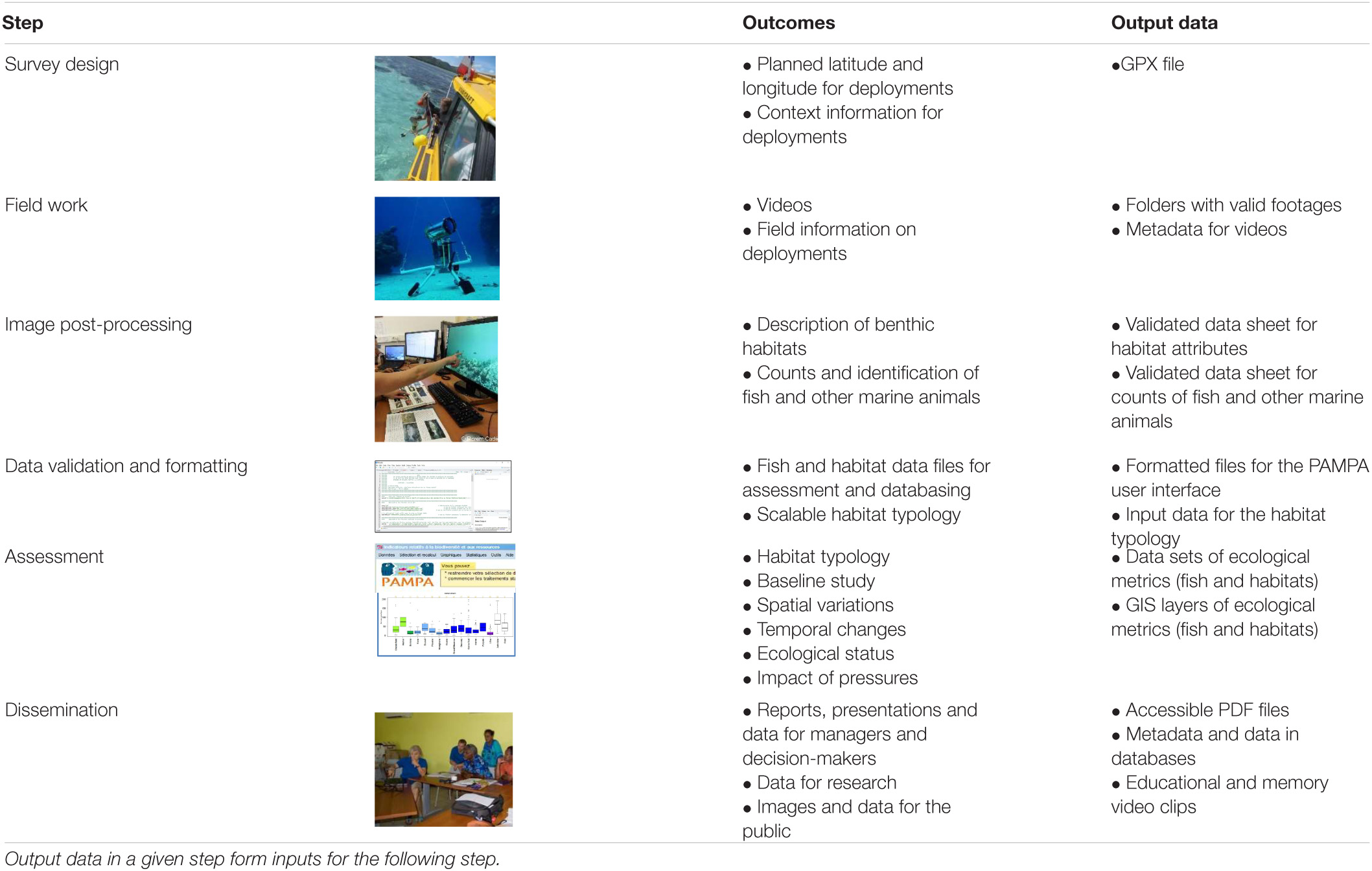
Table 1. Steps of the workflow with corresponding outcomes and output data.

Survey Design

The survey design covers the entire area of interest with a systematic distribution of the observations stratified according to habitat and anthropogenic pressures or protection status. The definition of sampling strata relies on existing maps and knowledge gained from the end-users, e.g., MPA managers or local communities. Habitat may encompass here geomorphology, benthic coverage types or exposure to waves and wind. Observations are distributed in each habitat with a higher sampling effort in habitats where biodiversity is more diverse and abundant, ensuring a better precision of derived estimators (Cochran, 1977). With respect to protection status, the survey design has multiple observations in each regulation zone of the MPA, and for anthropogenic pressures, in zones bearing distinct pressure levels. Baseline assessments typically involve a larger number of observations than follow-up surveys. The design is generated on a GIS (e.g., QGIS Development Team, 2021), and the resulting latitudes and longitudes are transferred to a portable GPS for field work. Establishing the sampling design for a baseline in a new area takes ca. two work days.

Field Implementation

The STAVIRO lander is dropped from the boat at the desired location and set horizontally on the seabed. To minimize disturbances due to boat presence, engine noise and lander drop and retrieval, the lander is left in situ for approximately 15 min so that images are recorded over three complete undisturbed rotations. The duration of an observation and the number of rotations recorded follow from extensive testing in 2007 and 2008.

Two landers are used together at nearby places to optimize time at sea. The number of observations that can be achieved per hour depends on the distance between stations; we recommend that the two landers are not set too far apart to minimize traveling distances. In a given day, corresponding to ca. 6 h of field work, a pair of systems can achieve an average of 20–40 deployments, depending on traveling time between stations, bottom rugosity, depth and weather conditions. Deployments require a skilled pilot and two or three crew with technical roles, with at least one trained for deployments, the other crew helping with the drops/retrievals and with the field sheet. In shallow depths (down to 15 m) and under good weather conditions, a pilot and one crew are enough.

Practical operational steps and checklists have been developed and are used to avoid errors and facilitate the uptake of the protocol by new operators (Supplementary Materials 1, 2). Pre-field work tasks include checking batteries and camera settings and closing the housings, while post-field tasks consist in rinsing the equipment with freshwater, loading the batteries and taking care of the images. Hence, after each sampling day or trip, images are downloaded on a laptop, and checked through a rapid screening process (derushing). A video is deemed valid for image analysis when: (i) underwater visibility (estimated from reference images, see below) is at least 5 m; (ii) the field of view is not obstructed by any sea floor or benthos relief that would prevent image analysis within a 5 m radius around the lander; and (iii) three complete undisturbed rotations are recorded. If (i) and (ii) are met for at least a complete rotation, the video is only analyzed for habitat, or else it is used either for communication purposes only, or discarded. Information from the derushing and field metadata are input in a standardized Excel spreadsheet (Supplementary Material 3). These metadata are critically needed for the effective management and analysis of large numbers of observations. The tasks inherent to pre- and post-field work each day, respectively take 1–2 and 3 h with two of the crew.

Image Post-processing

For each valid video, habitat attributes (Table 2) are evaluated from a single rotation for an estimated 5 m radius around the lander, corresponding to an observed surface area of ca. 78.5 m². Habitat attributes are evaluated in each frame of the rotation (Supplementary Material 4).

TABLE 2

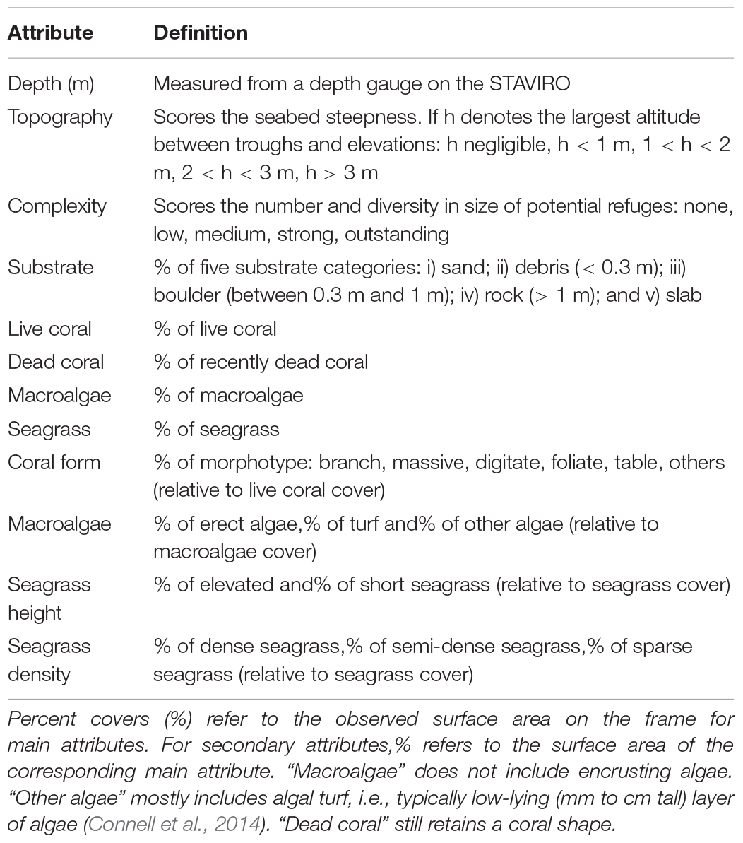
Table 2. Habitat attributes annotated on each frame of a footage for coral reef ecosystems.

Fishes and other marine animals (termed herebelow macrofauna) are identified at the most precise taxonomic level based on a reference species list (see below), and counted on each frame and for each of three successive undisturbed rotations within a 5 m radius around the system (Supplementary Material 5). To minimize disturbance, counting starts once a complete rotation has been achieved after the lander is set on the bottom.

The species list is cross-referenced with WoRMS (Horton et al., 2021). In coral reef ecosystems, two reference lists were constructed. The most exhaustive list includes families that have at least one species that inhabits reef and lagoon areas in depths in the 0–50 m range, i.e., 56 families (Table 3), and excludes cryptic, nocturnal and buried species, as well as species with Lmax smaller than 18 cm as determined from FishBase (Froese and Pauly, 2019). The list comprises fishes, turtles and sea snakes (see Pelletier et al., 2016 for details). For species that may be confused, species complexes were defined jointly with Underwater Visual Census (UVC) fish experts. From this first “complete” list, a second reference list focuses on species that are either fished, iconic, protected, or of particular ecological significance. This second list is used for instance when the assessment is focused on fishing resources. In temperate ecosystems, all species that are not cryptic, nocturnal or buried are identified and counted.

TABLE 3

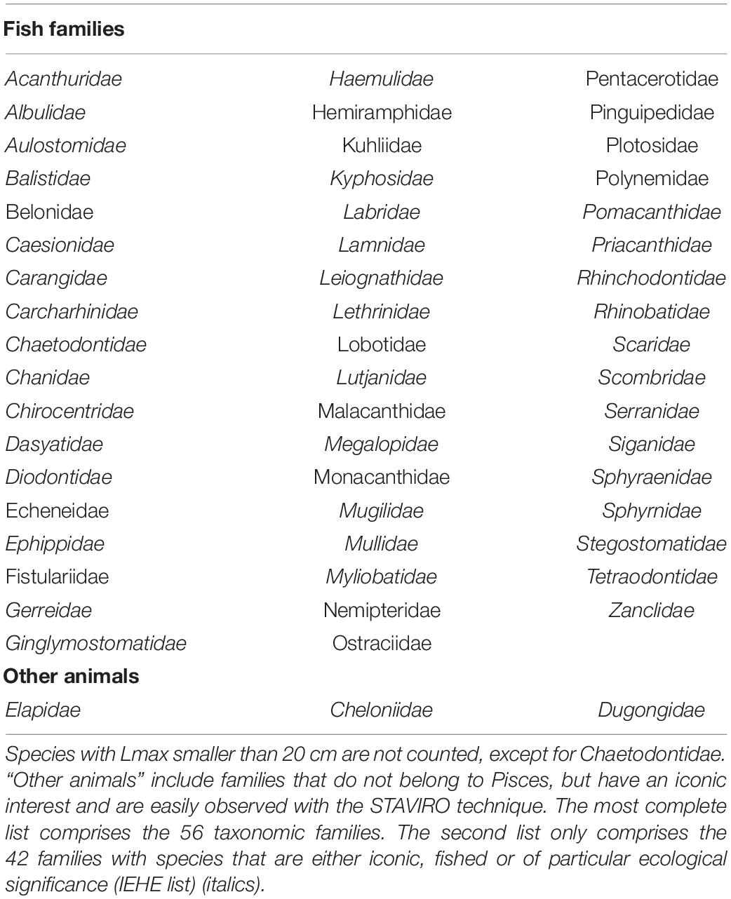
Table 3. Species lists considered for counts in image analysis.

Animals are identified to species level or alternatively at genus or family level. A snapshot or short video clip is sent to experts, or to collaborative tools such as iNaturalist⁵, if identification needs confirmation. Quality assurance for image analysis relies on the training of analysts. Each analyst conducts joint annotations with an expert. For fish counts in coral reef ecosystems, training takes up to 1 month. Training is validated after successful joint analyses of a set of videos. In parallel, 5% of the videos are independently reviewed by an expert analyst. If identifications and counts differ by more than 10%, the video must be reanalyzed. Attention is paid to species that may be potentially confused with one another. Estimation of visibility and 5 m radius followed training of annotators with calibrated reference images comprising bright and dark fish silhouettes of several sizes filmed at a range of distances and in several visibility conditions. The template file for animal counts comprises several fields to record the time code and the position of the animal on the frame, in order to ease quality control and to anticipate the future making of annotated image databases for machine learning (ML) algorithms (see section “Information Gained from Images”). Finally, once the set of videos has been analyzed and controlled for quality, the data are checked for inconsistencies using R scripts developed for this purpose.

Analyzing a video requires 10–90 min for identifying and counting macrofauna depending on diversity and abundance, and 15 min for habitat description. This is achieved by a trained person and facilitated when a second person inputs the data.

EBV Production and Analyses

The data tables resulting from the macrofauna counts and the field metadata are then, respectively formatted following the PAMPA template into a file for counts and a file with the metadata per observation unit. The abundance per taxon is computed by the PAMPA UI for each observation as the mean count over three rotations (within 5 m around the camera), which averages out the variability between rotations. Abundance is expressed in densities (numbers of individuals per 100 m², ind/100 m²). Species richness is the total number of species observed within 5 m around the camera during the three rotations. The interface also computes other diversity indices such as Shannon’, Pielou’s, Simpson’s, and Hill’s (Hill, 1973). A wide array of abundance and diversity metrics may be easily calculated based on a range of species-specific taxonomy, trait and use-related criteria. Habitat-related metrics such as biotic covers may also be analyzed through the UI. Biotic cover per observation unit is defined as the mean percent cover of the biotic category (i.e., macroalgae, sea grass, or live coral) averaged over the six frames of the analyzed rotation.

Habitat data are moreover formatted in a data table to construct a habitat typology based on clustering and classification (Pelletier et al., 2020). This typology defines the local habitat to each observation unit as a covariate for spatial and temporal differences e.g., in fish abundance and diversity. This is important because observation units are collected in various habitats, and the distribution of mobile macrofauna is strongly linked to habitat distribution.

Metrics are efficiently computed, plotted and analyzed with GLMs using the PAMPA UI, and now with the Galaxy-E web platform (Supplementary Material 6). GLMs test for the effect of either protection status or anthropogenic pressure, while accounting for local habitat derived from the typology. Where several years of data are available, temporal changes are tested too.

EBV Products for End-Users

Several EBVs and EOVs are documented by this protocol (Table 4) and their spatial replication enables the distribution of variables inherent to both EOVs and EBVs to also be assessed.

TABLE 4

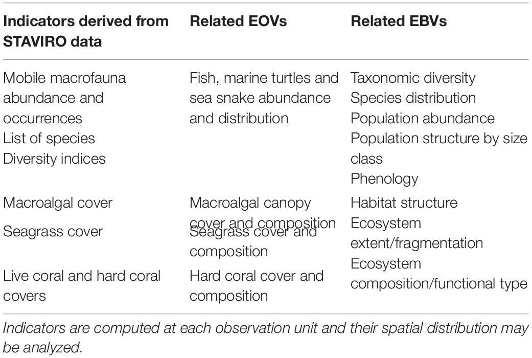
Table 4. Link between EOVs and EBVs, and the indicators derived from STAVIRO data.

Applications for the STAVIRO protocol first include assessments linked to human activities and interventions: (i) MPA effectiveness, i.e., tracking progress toward biodiversity conservation and sustainable fishing goals; and (ii) assessment of the impact of anthropogenic pressures, among which recreational and commercial uses of coastal areas, industrial projects, urbanization and marine renewable energies. In each use case, a baseline survey is conducted to establish the spatial distribution of EBVs and test the differences between zones with distinct protection levels, regulations of uses, and anthropogenic pressures. Follow-up assessments involve testing both spatial and temporal variations of EBVs according to the same factors.

The second application type deals with assessing ecosystem health or biodiversity status against conservation objectives at the scale of territories or wide areas. With numerous data collected in varied habitats subject to contrasted anthropogenic and environmental pressures, the distribution of EBVs is representative and may be mapped at the scale of the site, area or territory. EBVs may be scored and assigned color codes per observation unit; five scores are used from red (bad) to blue (excellent). For each EBV, scores are then averaged at the scale of each surveyed site and organized into aggregated radarplots. Such concise displays enable straightforward comparison of ecological status across sites within a given region.

In both applications, the conservation goals considered follow from previous projects with MPA managers (Pelletier, 2020a): (i) sustainable exploitation of resources and (ii) conservation of biodiversity with four objectives targeting: communities and species representative of the ecosystem, ecosystem functions, species of particular significance, and representative habitats. Indicators are selected according to their relevance to the conservation objectives, and analyzed depending on habitat, local anthropogenic pressures and protection status following a template (Supplementary Material 7). EBV maps are obtained by exporting georeferenced metrics from the PAMPA UI toward GIS layers. In addition to the indicators, the list of species and the relative frequencies of dominant families document the Taxonomic Diversity EBV. Lastly, each baseline assessment includes a recommended sampling design for follow-up surveys. Additional information reported with the assessment for quality assurance and transparency comprise the percentage of valid drops, the percentage of individuals identified at species, genus and family levels, and the time spent for image analysis.

The third application of the STAVIRO data lies in a variety of research studies, including biogeographic studies, socio-ecosystems analysis and modeling, as well as studies of fish behavior and interspecific relationships enabled by the unobtrusiveness of the lander.

Dissemination of Outcomes and Data Management

The STAVIRO protocol generates spatially replicated EBV and a large number of observations. GIS-layers of EBVs are hosted on an institutional Open Access map serve⁶. Quantitative data issued from image analysis are uploaded on institutional databases and/or shared to other initiatives for data sharing. Assessment reports are systematically posted on the Open archive https://archimer.ifremer.fr/search. Image data are safeguarded through archives on institutional databases servers and duplicated on local hard drives.

Two types of image-based outcomes are produced: (i) a video clip assembling short sequences recorded at a subset of representative stations, yielding a memory of the ecological status of the area at the time of the survey; (ii) a compilation of outstanding images that either depict the biodiversity assets inherent to the area, in order to provide end-users with a better knowledge of the values to be protected in the area; or display areas under critical anthropogenic pressure. Image-based outcomes of interest to a broader audience or helpful to complement assessments or research outcomes are posted on the image portal https://image.ifremer.fr/.

Applications

The wide range of applications of the STAVIRO protocol—four ecosystems located in three oceanic regions: the Southwest Pacific (New Caledonia), the Indian Ocean (Reunion and Mayotte Is.), the Northwestern Mediterranean Sea and the Atlantic Ocean—is illustrated in Figure 2 and Table 5. Between 2007 and 2020, more than 4500 observations were collected to assess fish and habitats to inform a range of conservation-related questions occurring at different spatial scales (Table 5) in a variety of ecosystems, habitats and depths (Table 6 and Supplementary Material 8). In New Caledonia and in the Indian Ocean, vast areas were sampled intensively over relatively short period of time, e.g., the Geyser Bank (230 obs., 7 days, Figure 3), Chesterfield and Bellona reefs and atolls (202 obs., 10 days), and the complex Corne Sud reefs (143 obs., 6 days) (Figure 4). 900 observations were sampled in the Mediterranean Sea along the French coast and in Corsica (Figure 5). Overall, the proportion of valid observations per survey lied between 80 and 95%, depending on weather conditions and water clarity. Example imagery is given in Figure 6.

FIGURE 2

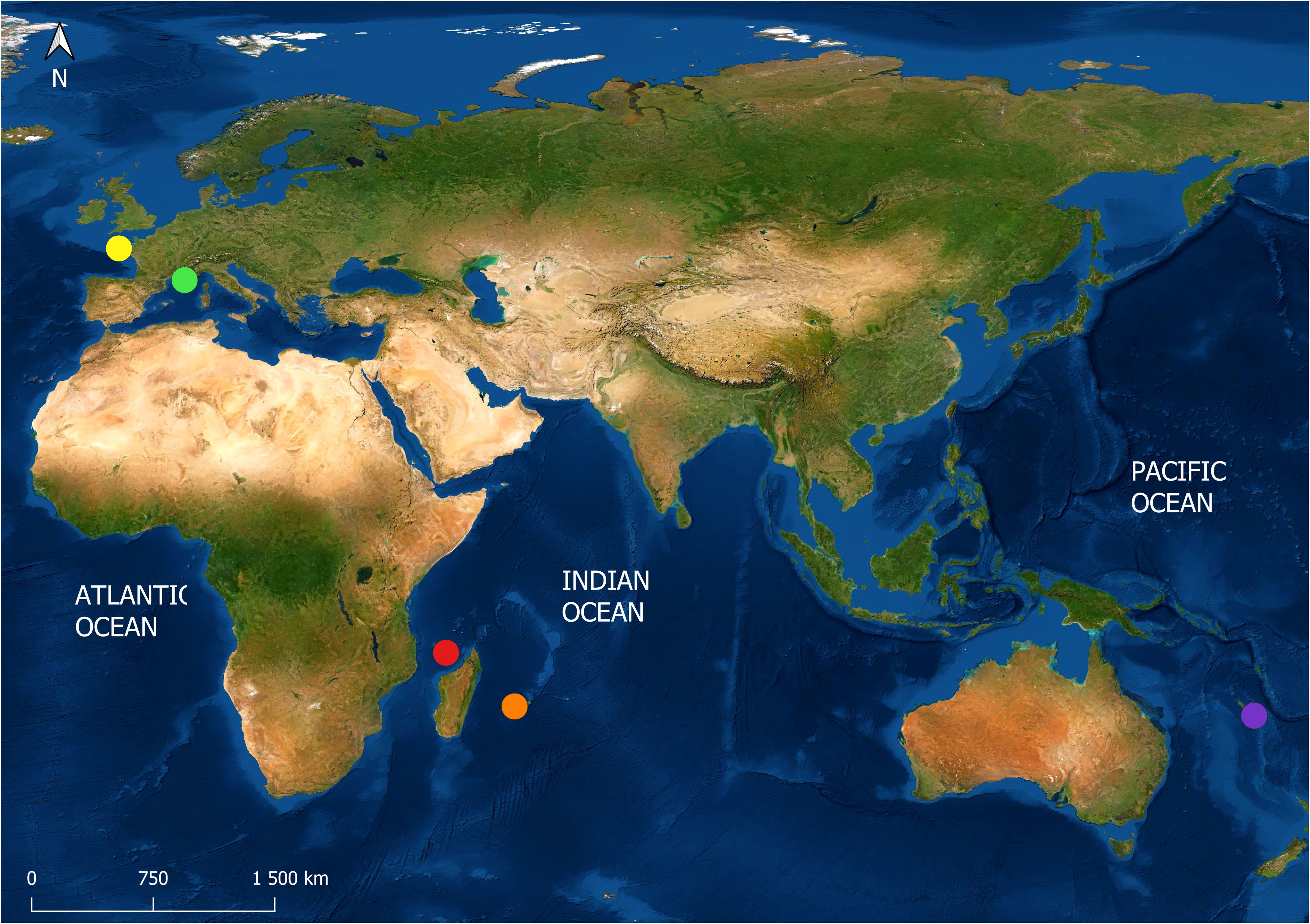
Figure 2. Regions where the STAVIRO protocol was implemented: New Caledonia (purple), Reunion Island (orange), Mayotte Island (red), Mediterranean Sea (green) and Atlantic Ocean (yellow).

TABLE 5

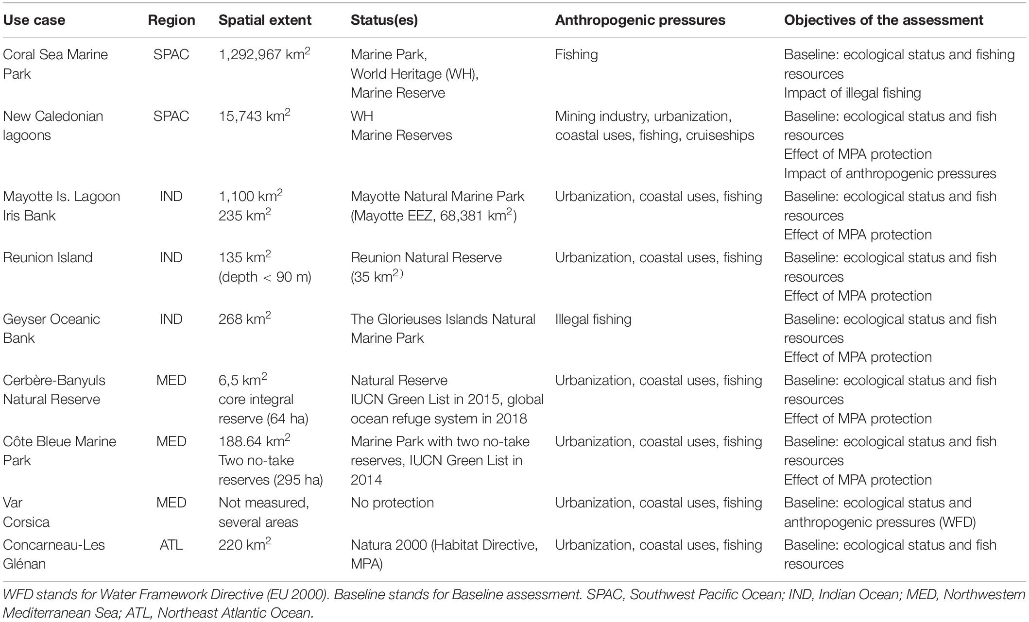
Table 5. Assessments conducted using the protocol.

TABLE 6

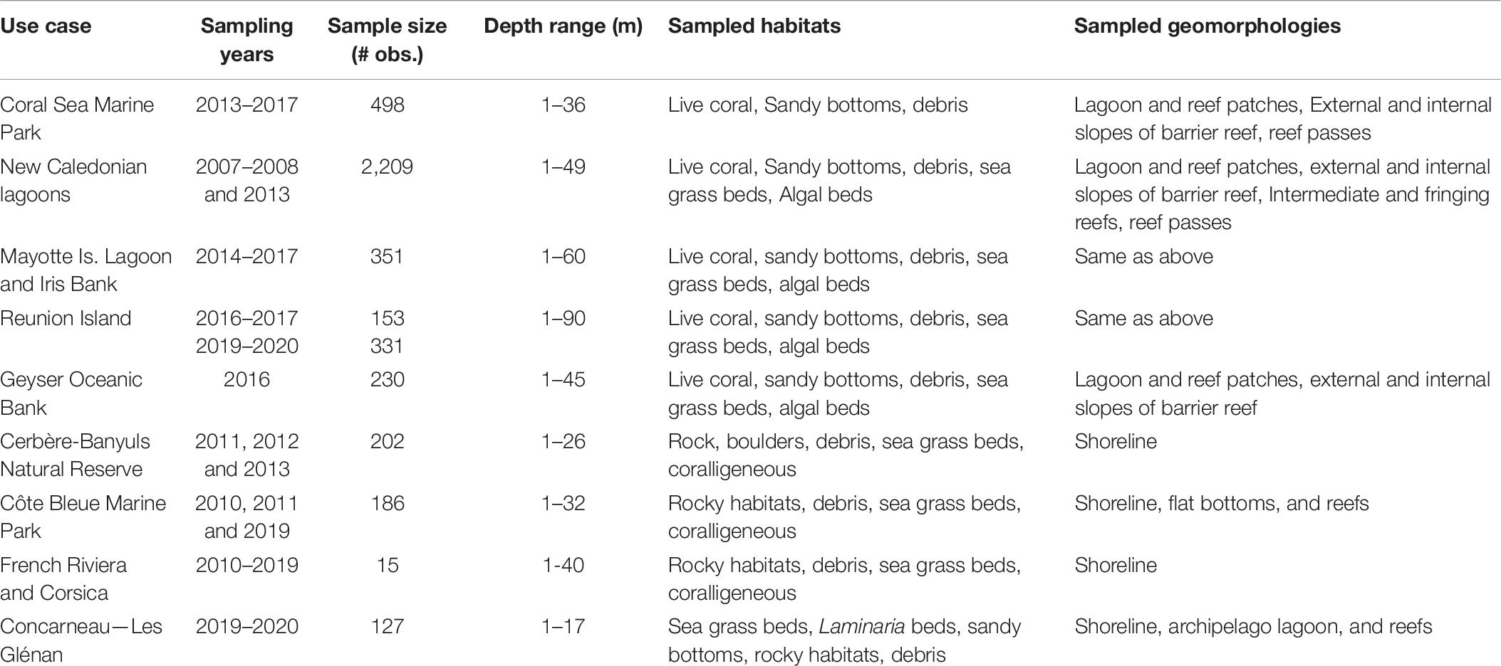
Table 6. Main features of samples for the use cases.

FIGURE 3

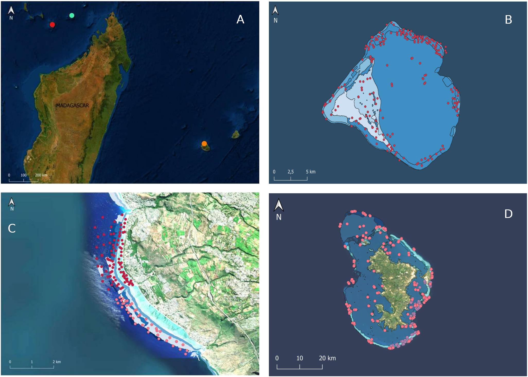
Figure 3. Sampled sites in the Indian Ocean (A) [Geyser Bank (light blue); Mayotte (red) and Réunion Island (orange)], and sampled stations in Geyser Bank (B), Réunion Natural Reserve (C) and Mayotte (D). At the Réunion Natural Reserve (C), sampling corresponds to 2016 (red) and 2017 (pink).

FIGURE 4

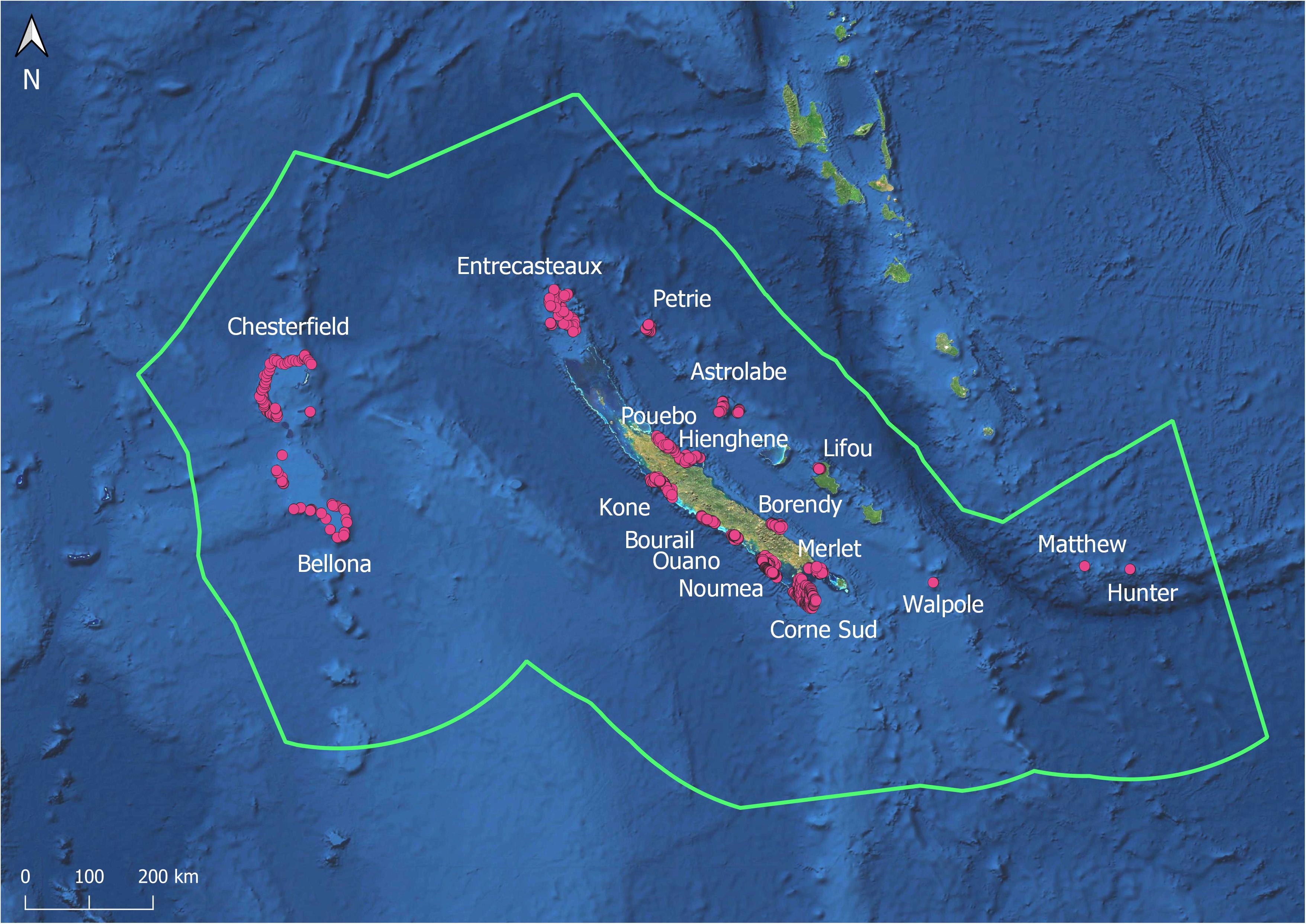
Figure 4. Sampled sites in New Caledonia. The Economic Exclusive Zone (EEZ) (green) also delineates the outer boundary of the Coral Sea Marine Park (CSMP) (Table 5). The CSMP inner boundary is the barrier reef surrounding the main island and the three islands of the Loyalty archipelago, (among which Lifou Island) located between Astrolabe and Walpole. Boundaries of the World Heritage property are in orange.

FIGURE 5

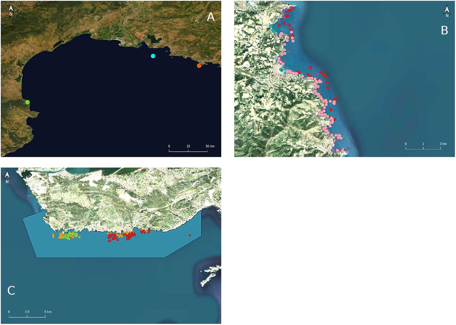
Figure 5. Main sampled sites in the Mediterranean Sea (A) (Cerbère-Banyuls Natural Marine Reserve (green), and Côte Bleue Marine Park (light blue), and Sicié Cape (orange) and sampled stations at the two coastal MPAs surveyed with the protocol: (B) Cerbère-Banyuls Natural Marine Reserve and (C) Côte Bleue Marine Park.

FIGURE 6

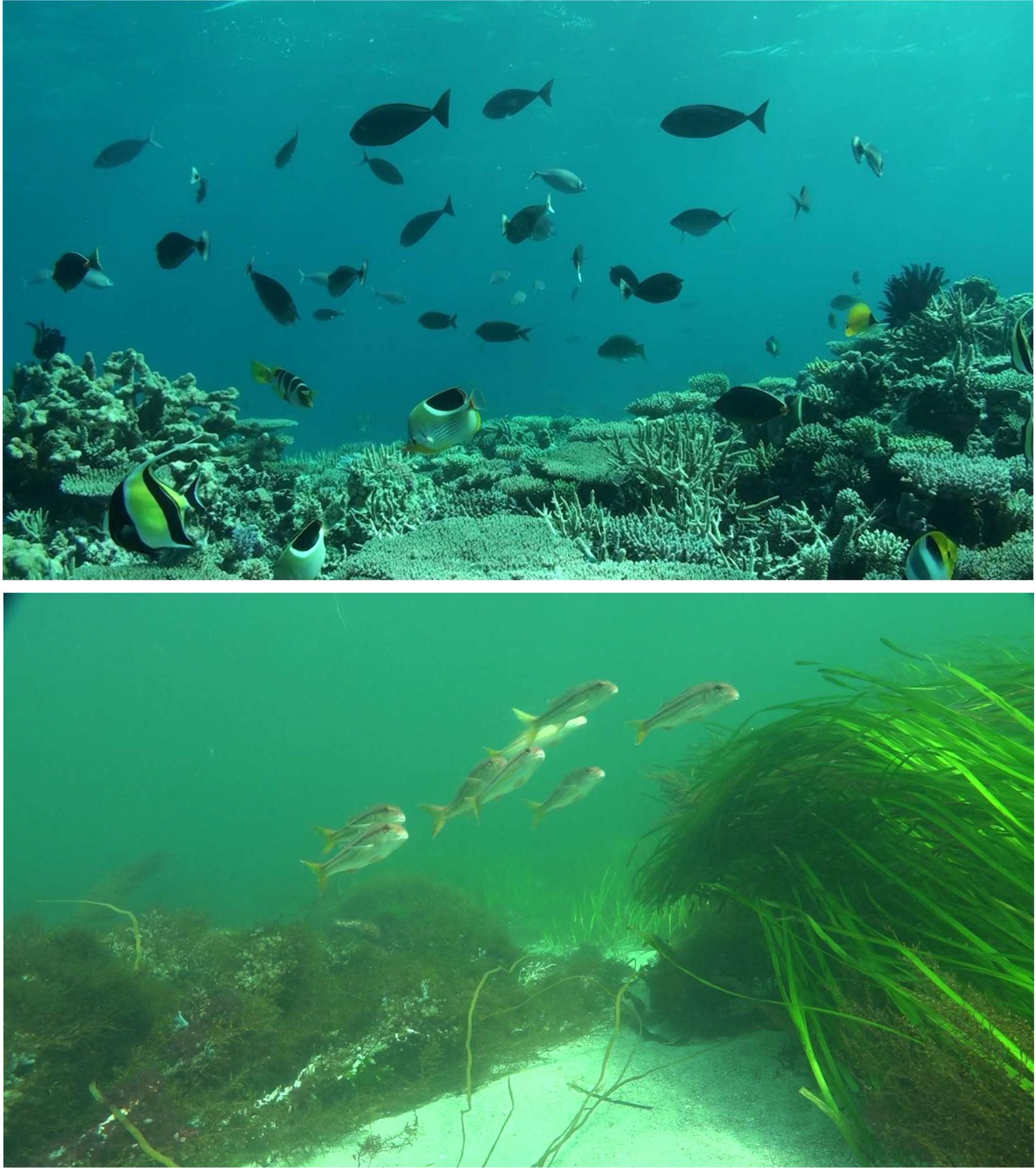
Figure 6. Example of images recorded by the STAVIRO. Top: Chesterfield reef, CSMP, New Caledonia. Bottom: Concarneau Bay, Atlantic Ocean.

EBV products and dissemination are illustrated by outcomes from New Caledonian data. A first EBV product for monitoring and assessment is habitat structure per observation unit, through (i) five main types of habitat (Sea grass beds, Macroalgae, Sandy bottoms, Live coral and Debris) and (ii) within each habitat type, rules describing heterogeneities at finer scale (Pelletier et al., 2020). Habitat structure is representative of the reef and lagoon habitats of New Caledonia’s EEZ (Figure 4) and was mapped at site (Figure 7) and region scale. In assessments of ecological status, habitat types better explained habitat-related variations of biotic covers, fish communities, and other marine animals, than e.g., geomorphological maps (Supplementary Material 8). As a second EBV product, 27 indicators for fishes and other animals, and four indicators for habitat-related EBVs form the basis for the assessments at each surveyed site (Table 7, link with EBVs and EOVs in Table 4). In addition, the main indicators were scored from ∼2,400 observations and used to compare the ecological status of reefs across the World Heritage sites, and within the Coral Sea Marine Park (CSMP) and (Figure 8 and Table 5). In the CSMP, our assessments contributed to update site-specific species inventories and revise the status of potential target species, e.g., in the Chesterfield and Bellona atolls and reefs (Supplementary Material 8). They also showed the exceptional health of Astrolabe’s reefs, which are now a fully protected integral reserve. The presence of iconic and keystone species was quantified, in particular in the CSMP where frequent occurrences and large abundances of sharks were observed in the absence of any bait. During presentations to stakeholders, managers or to the public, screenshots and short clips illustrated scores and figures in a simple way. Lastly, the New Caledonian habitat data were part of the reference samples used in ML-based mapping of coral habitats for the Allen Coral Atlas⁷.

FIGURE 7

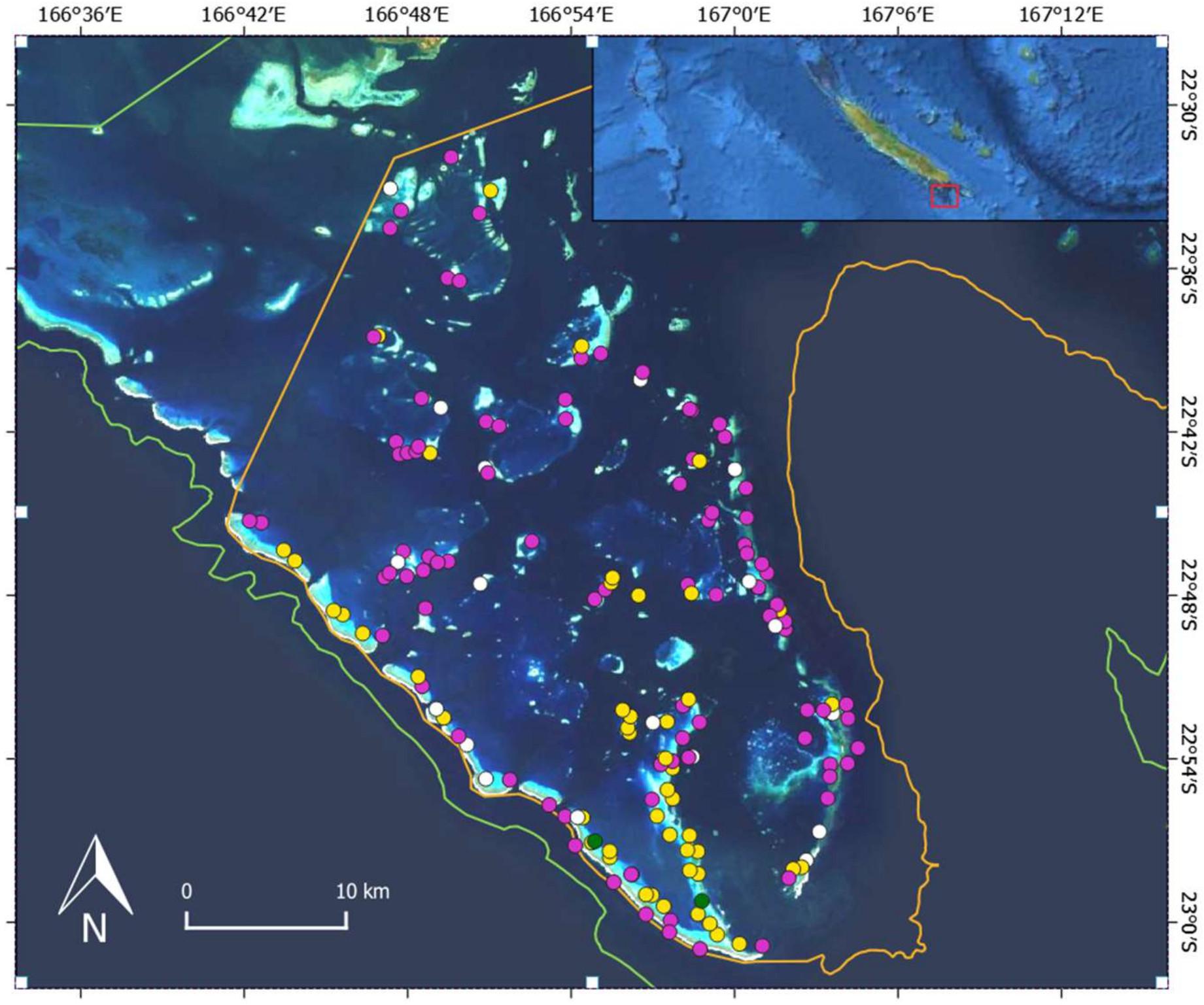
Figure 7. Distribution of habitat types in the Corne Sud, World Heritage property (from Pelletier et al., 2020). The habitats observed in this area are: Live coral (pink), Debris (white), Sandy (yellow). The orange line delineates the Southern Lagoon World Heritage Property.

TABLE 7

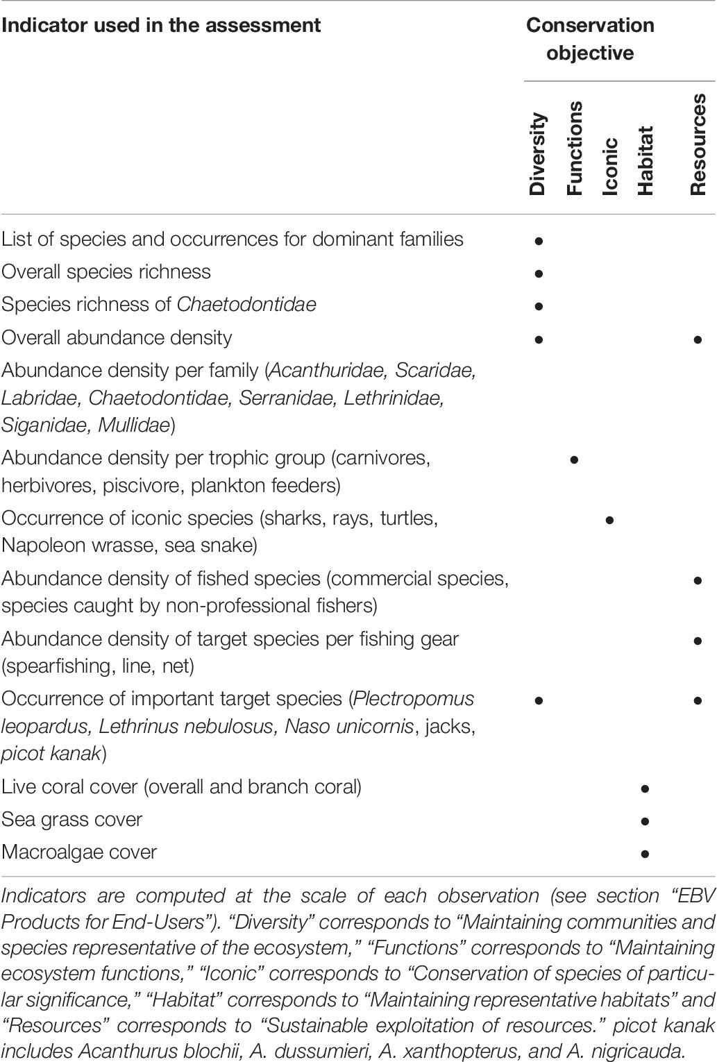
Table 7. Indicators derived from STAVIRO data collected in New Caledonia to document EBV related to mobile macrofauna in the light of tracking progress toward conservation objectives.

FIGURE 8

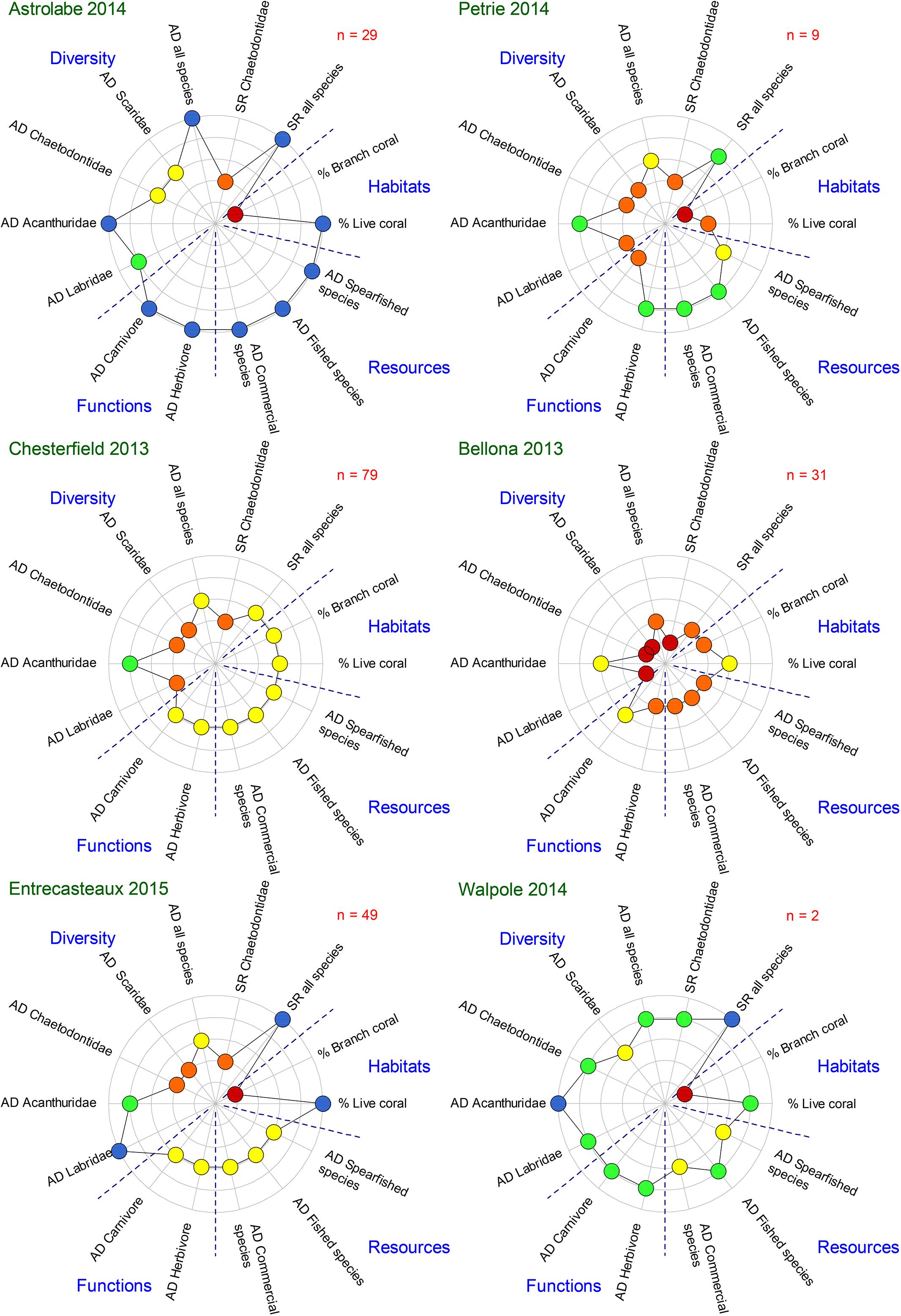
Figure 8. Cross-site comparison of ecological status of the main reef areas in the Coral Sea Marine Park, New Caledonia. The locations of the reefs are showed on Figure 4. AD and SR stands for abundance density and species richness, respectively.

Many research opportunities are supported by the wealth of data provided by STAVIRO, in particular, statistical modeling requiring spatially distributed and replicated data, for example, species distribution modeling, spatial patterns of habitats (Pelletier et al., 2020) and relationships between species and environmental variables (Powell et al., 2016; Garcia et al., 2018). The programmable version of the STAVIRO, the MICADO, is suited for longitudinal studies, e.g., of short-term variations of fish abundance (Mallet et al., 2016) and phenological processes such as spawning aggregations (Pelletier D., unpublished data).

Lastly, our work has resulted in the production of communication and outreach material: image sets (Pelletier, 2020b), educational conferences and video clips that are freely available on YouTube, at https://www.seanoe.org/and at https://image.ifremer.fr/search.

Discussion

The STAVIRO protocol—all steps from data collection to knowledge production and dissemination—has been applied in various settings over a period of 12 years. This enabled the different steps of the workflow to be adapted to the final goal of EBV and EOV production. The protocol has both advantages and limitations relative to other observation protocols, and these are discussed below, as well as perspectives.

Non-obtrusive Observation

Like all video-based observation techniques, the STAVIRO is non-extractive which is an advantage for assessments, particularly in areas that are protected or host vulnerable biodiversity. As a lightweight lander, it has no impact on benthic habitat, is inconspicuous, and is unbaited, resulting in a minimal effect on the behavior of fishes and other mobile macrofauna. This is an advantage compared to diver-operated observation techniques like UVC and DOV that may be prone to differences between observers (for UVC), and to diver avoidance by some species (Kulbicki et al., 2010; Dickens et al., 2011). In a paired experiment, the STAVIRO observed more individuals from large species and target species than UVC (Mallet et al., 2014). This minimal disturbance is also an advantage for studying animal behavior and interspecific relationships, and the automatic version of the STAVIRO has been used for this purpose (Mallet et al., 2016; Pelletier, unpublished data).

Easy and Fast Deployments

This lightweight lander is easily deployed from diverse boat types, which has fostered the participation of diverse operators, e.g., in New Caledonia, people from the management committees, commercial fishers and rangers. Hence, field work can be realized by non-expert staff entailing (i) reduced personnel costs on the field (no need of expert divers or researchers); and (ii) the potential to engage into participative and citizen-based approaches, and encouraging knowledge exchange and capacity building.

Another strength of the STAVIRO protocol is its ability to survey large areas and obtain spatially replicated data for statistical analyses, as many observations can be collected per day at sea. Most habitats may be surveyed and depth is hardly a limitation (within the euphotic zone) when compared to diver-operated techniques which are constrained by both depth and time taken per observation. Shallow water BRUVs also typically have a deployment time of 1 h.

Yet, the fine-scale positioning of the STAVIRO system requires training for the crew and pilot, as the lander must be horizontal with no obstacles around, sometimes in deep water and navigating in wind and waves. To date, just a single camera housing was damaged during thousands of stations. The lander is very stable and the entanglement of the rigging during the observation, generally due to currents, is quite rare and is completely avoided by a rigid rigging.

Field of View and Panoramic Video

The frames recorded by the rotating camera are similar to the field of view of human eyes, thereby minimizing image distortion entailed by wider angles of view. This feature and the horizontal view facilitate image analysis for both mobile animals and benthic covers. The panoramic view together with the 60° angle of view enables to characterize habitat and count animals at a distance of at least 5 m and to compute abundance densities (and not only relative abundance indices). We acknowledge that the estimation of the 5 m distance is subject to some uncertainty, as the STAVIRO does not use stereo video (but see section “Information Gained From Images”); however, this uncertainty is minimized by the training of analysts and the reliance on reference images.

Information Gained From Images

Image post-processing has, to date, been carried out manually by trained analysts. This step of the workflow is time consuming due to the large number of videos collected and the substantial processing time per video. Double counting and missed animals are possible for any observation technique where the entire seascape is not simultaneously observed over a 360° field of view, but were minimized at each step of the workflow: (i) in early deployments, the duration of each fixed frame, the angle and speed of rotation were adjusted to the movements of the observed fauna; (ii) during image analysis, attention is paid to the direction of the moving animals and any animal potentially déjà vu is not counted; and (iii) animal abundance computed as a mean count over three rotations smoothes out variability due to moving animals. This estimate is analogous to the MeanCount statistic sometimes used instead of MaxN for BRUV (Campbell et al., 2015; Stobart et al., 2015).

An acknowledged drawback is that our protocol provides coarse and visually estimated size classes, not precise size information. To circumvent this, a stereo version of the system was trialed, but it is bulkier on board and deployments were relatively slow. A second stereo version is currently being developed. A mixed protocol could be implemented in which spatial cover and replication is achieved via the current lander, and a subset of the observations using a stereo version provides size-based information and distance measurements.

Video imagery enables annotators to work collaboratively to ensure that identifications are consistent and relies on an iterative and somewhat time-consuming process (Langlois et al., 2020). Our current procedure for image post-processing, both collaborative and iterative, is effective. Possible differences between analysts as well as uncertainties about size class and surface estimation are handled in a conservative and prudent manner, during post-processing and in the choice of indicators, e.g., most of the indicators used in assessments are not at species level.

In terms of observed taxa, the STAVIRO cannot capture cryptic and nocturnal species, just like UVC or other video-based protocols. In addition, the panoramic video differs from BRUV or UVCs which recording animals at close distances: small species are not observed in a consistent way up to a 5 m distance. These species are thus either excluded from the counts in diversified coral reef ecosystems, or from data analyses in other ecosystems. In addition to the two species lists for coral reef ecosystems (section ‘‘Image Post-processing’’), a simpler list was devised based on the species groups considered in the participative Reef Check protocol⁸. This list enables citizen involvement in image analysis, but was not used in our assessments. Web-based tools are also currently being developed for citizen-based image annotation (Matabos et al., 2016).

The next improvement in our protocol lies in the use of annotation tools for direct annotation, and for constructing databases of images for ML algorithms. We have successfully used the EventMeasure software (seagis.com.au) and are investigating adapting BIIGLE (Langenkämper et al., 2017) for video imagery. Our archived data enable to build training data sets to implement ML-based approaches in future applications.

Lander Reproducibility

One drawback in the light of long-term monitoring is the lander’s dependence on commercial cameras which evolve over years and are replaced by different models, thus requiring the housing or electronics to be adapted and incurring undesirable costs. Because this may be an obstacle to the adoption of the system by other workers, the KOSMOS project was commenced in 2020 to re-develop the STAVIRO (and the MICADO), as a fully Open Source, reasonably costed tool that provides images compatible with the previous version. KOSMOS focuses on the assembly of essential parts, i.e., lens, sensor, housing, electronics and processor, in a more compact system and bypasses the irrelevant features of commercial cameras. Its design and fabrication is a collaborative project⁹ implemented with a French FabLab, i.e., a digital fabrication laboratory providing access to the environment, skills, materials and technology to allow volunteers to create, learn and innovate¹⁰. A prototype was recently successfully tested. The cost of the complete system will range between 1000 and 1,500 euros, and will make the entire STAVIRO protocol become Open Source and reproducible by a wide audience.

EOV/EBV Data Products and Dissemination

Through simultaneous observations of fishes, habitats and some other marine animals such as turtles and sea snakes, the STAVIRO protocol documents several EBVs: taxonomic diversity, population abundance (with additional information per size-class), habitat structure, ecosystem composition (and functional type) and phenology. Medium to large size mobile animals are well observed (section “Non-obtrusive Observation”). Relationships between habitat and macrofauna may be studied through paired information. However, the STAVIRO protocol is not the most appropriate protocol for counting small species and semi-cryptic species concealed in coral, crevasses or under rocks. It may thus be used in combination with a complementary monitoring protocol, in which case protocols should be intercalibrated. For instance, participative UVC sampling schemes deployed over large areas such as Reef Life Survey (Edgar et al., 2020) offer opportunities for spatial coverage. BRUVs are another avenue to reveal some cryptic species that may be attracted by bait.

By collecting many deployments per day at sea with only two STAVIRO units, the protocol provides replicated data over large areas, thereby informing distributional EBVs such as species distribution, ecosystem extent and fragmentation. Standardization is indispensable not only for data quality and reproducibility, but also for effective management and analysis of these big datasets. The PAMPA UI was central for operationalizing the production and analysis of EBVs, and coding the PAMPA workflow on Galaxy-E (section “Software for EOV/EBV Production”) facilitates data re-use.

Our video-based assessments provide unique baseline studies for areas that had been poorly surveyed before, either because they were remote, too deep, or too vast. Designs that encompass the main habitats encountered in the surveyed area enable the distributions of species to be characterized according to habitat and geomorphology. In combination with replicated observations across areas subject to distinct pressures and protection status, a comprehensive and statistically robust assessment can be obtained. Because of both high sampling effort, large coverage and sampling in all habitats, the assessments provide a holistic view of the surveyed area. In addition, the standardized protocol makes these assessments scalable to large territories and comparable across sites.

A central motivation is to make the protocol, workflow and data visible, traceable and accessible for scalable assessment and research. With imaging, raw (images) and annotated data (counts and habitat description) may be archived, shared, and re-analyzed for similar or different objectives. Given the efforts invested in data acquisition and image post-processing, sharing the resulting data is an obvious necessity.

To satisfy the principles of Open Science (Kissling et al., 2018), each step of the workflow can be achieved from freeware, data are progressively made FAIR, data management links raw data, processed data and outcomes including dissemination, and data will be eventually uploaded to international biodiversity archives, e.g., OBIS¹¹.

Equally important to promote the use of the protocol to scientists and other end-users for monitoring and assessment are the dissemination and capacity building activities. Our end-users included environmental managers and agencies (e.g., MPA staff), participatory management committees, fishers and private operators. In addition to staff from academia and environmental agencies, a number of people were trained in the four regions sampled and became private operators for monitoring and for research.

A final and important aspect of dissemination lies in outreach. Image-based products proved useful for communicating results to most audiences for several reasons: (i) they conveniently illustrate numerical and graphical outcomes; (ii) imagery-based evidence facilitates knowledge exchange with local management committees and the public, who discover or revisit “their” marine biodiversity and resources (Pelletier, 2020a), and (iii) from an educational standpoint, images provide a sense of pride and custodianship about “their’ territory, with positive consequences for caring about the environment. In our protocol, fishes and animals behave in a natural way and show undisturbed behaviors which have raised the interest of many viewers.

Conclusion

The standardized STAVIRO protocol and workflow have been fully operationalized through extensive and successful implementation in a variety of contexts, including at the scale of vast managed areas. The imagery, annotation and the derived EBV products and outcomes support assessments of coastal fish assemblages and habitats in a robust and effective way according to procedures that are evolving toward meeting FAIR principles. In future years, the protocol will support: (i) additional technology to optimize collection of imagery, (ii) software developments, especially machine learning, to facilitate image post-processing and annotation; and (iii) enhanced interoperability with other researchers and stakeholders.

This paper aims to help using the protocol by sharing our extensive experience, the data collected and the savoir-faire gained since 2007. As a versatile and accessible protocol, it can be applied in diverse contexts for monitoring, research and educative needs. The STAVIRO’s proven track-record of utility and cost-effectiveness indicates that it should be considered more broadly for future applications.

Data Availability Statement

The original contributions presented in the study are included in the article/Supplementary Material, further inquiries can be directed to the corresponding author/s.

Author Contributions

DP conceived the STAVIRO protocol, the workflow and the manuscript. DP, DR, and MB led extensive surveys and assessments in the different regions and they tested and consolidated the protocol with the help of WR, CG, TB, LC, TS, BP, AP, JG, MG, and FC. YR developed and maintain the PAMPA user interface. CR and YL developed the Galaxy-E PAMPA application for STAVIRO data. DP wrote the manuscript. All authors have contributed to the writing and editing of the manuscript.

Funding

New Caledonia data were collected during (i) the PAMPA project with the support of the Research Institute for Development; and (ii) the AMBIO project funded by both IFREMER, New Caledonia Government and Provinces, the Conservatoire des Espaces Naturels of New Caledonia, and the French Ministry of Ecology, the French Initiative for Coral Reefs (IFRECOR), and the French Marine Protected Area Agency. Mediterranean data were collected with the support of IFREMER, the Cerbère-Banyuls Natural Marine Reserve, the Côte Bleue Marine Park and the French Water Agency. In the Indian Ocean, data collection was co-funded by Ifremer and by (i) the Reunion Marine Natural Reserve (PECHTRAD project), (ii) the Mayotte Marine Natural Park (Staviro Mayotte project), (iii) the 10th European Development Fund (FED), the Departmental Collectivity of Mayotte, the French Southern and Antarctic Lands and the University Center of Mayotte (EPICURE project), (iv) the European Fund for Maritime Affairs and Fisheries (FEAMP) and the French government (IPERDMX project).

Conflict of Interest

The authors declare that the research was conducted in the absence of any commercial or financial relationships that could be construed as a potential conflict of interest.

Publisher’s Note

All claims expressed in this article are solely those of the authors and do not necessarily represent those of their affiliated organizations, or those of the publisher, the editors and the reviewers. Any product that may be evaluated in this article, or claim that may be made by its manufacturer, is not guaranteed or endorsed by the publisher.

Acknowledgments

We thanks to the numerous collaborators who helped with field work, image analysis, managing and analyzing the data collected since 2007 among which: in New Caledonia: Kévin Leleu, Delphine Mallet, Charlotte Giraud-Carrier, Fanny Witkowski, Cyrielle Jac; in la Réunion: Johanna Herfaut and Paul Giannasi from the Mayotte Natural Marine Park; in the Mediterranean Sea: Gilles Hervé, Jérémy Pastor, Eric Charbonnel; and in the Atlantic Ocean: Claude Merrien and Aouregan Terre-Terrillon. We thank Eric Charbonnel, Jérôme Payrot, Jérémy Pastor, and Philippe Lenfant for facilitating the survey in the Banyuls and Côte Bleue MPAs. We thank Eric Charbonnel, Jérôme Payrot, Jérémy Pastor and Philippe Lenfant for their great help during the survey in the Banyuls and Côte Bleue MPAs.

Supplementary Material

The Supplementary Material for this article can be found online at: https://www.frontiersin.org/articles/10.3389/fmars.2021.689280/full#supplementary-material

Supplementary Table 1 | Checklist for field work and naming convention for the video files.

Supplementary Table 2 | Datasheet for field work.

Supplementary Table 3 | Metadata for each deployment and video.

Supplementary Table 4 | Datasheet for habitat (coral reefs).

Supplementary Table 5 | Datasheet for fish counts.

Supplementary Table 6 | Galaxy-E workflow implementing part of the PAMPA UI.

Supplementary Table 7 | Standardized template for indicator analysis.

Supplementary Table 8 | List of assessment reports in New Caledonia and Indian Ocean.

Footnotes

1. ^ https://www.plastimo.com/en/powerboat-engine-access/fishing-angling-equipment/fishing-angling-accessories/aquascope-demontable.html
2. ^ https://ecology.usegalaxy.eu/
3. ^ https://training.galaxyproject.org/training-material/topics/ecology/tutorials/PAMPA-toolsuite-tutorial/tutorial.html
4. ^ https://ecology.usegalaxy.eu/datasets/11ac94870d0bb33a5383255468c716b2/display/
5. ^ https://www.inaturalist.org/
6. ^ https://sextant.ifremer.fr/
7. ^ https://allencoralatlas.org/
8. ^ https://www.reefcheck.org/
9. ^ https://wikifactory.com/@gheleguen/kosmos-20-r%C3%A9alisation
10. ^ https://fabfoundation.org/
11. ^ https://obis.org/

References

Campbell, M. D., Pollack, A. G., Gledhill, C. T., Switzer, T. S., and DeVries, D. A. (2015). Comparison of relative abundance indices calculated from two methods of generating video count data. Fish. Res. 170, 125–133. doi: 10.1016/j.fishres.2015.05.011

CrossRef Full Text | Google Scholar

Cochran, W. G. (1977). Sampling Techniques, 3rd Edn. New York, NY: Wiley.

Google Scholar

Dickens, L. C., Goatley, C. H. R., Tanner, J. K., and Bellwood, D. R. (2011). Quantifying relative diver effects in underwater visual censuses. PLoS One 6:e18965. doi: 10.1371/journal.pone.0018965

PubMed Abstract | CrossRef Full Text | Google Scholar

Edgar, G. J., Cooper, A., Baker, S. C., Barker, W., Barrett, N. S., Becerro, M. A., et al. (2020). Reef Life Survey: establishing the ecological basis for conservation of shallow marine life. Biol. Conserv. 252:108855. doi: 10.1016/j.biocon.2020.108855

CrossRef Full Text | Google Scholar

Froese, R., and Pauly, D. (2019). FishBase. World Wide Web Electronic Publication. Available online at: www.fishbase.org (accessed January 30, 2020).

Google Scholar

Garcia, J., Pelletier, D., Carpentier, L., Roman, W., and Bockel, T. (2018). Scale-dependency of the environmental influence on fish β-diversity: implications for ecoregionalization and conservation. J. Biogeogr. 45, 1818–1832. doi: 10.1111/jbi.13381

CrossRef Full Text | Google Scholar

Goetze, J. S., Bond, T., McLean, D. L., Saunders, B. J., Langlois, T. J., Lindfield, S., et al. (2019). A field and video analysis guide for diver operated stereo-video. Methods Ecol. Evol. 10, 1083–1090. doi: 10.1111/2041-210X.13189

CrossRef Full Text | Google Scholar

Hill, M. O. (1973). Diversity and evenness: a unifying notation and its consequences. Ecology 54, 427–432. doi: 10.2307/1934352

CrossRef Full Text | Google Scholar

Horton, T., Kroh, A., Ahyong, S., Bailly, N., Boyko, C. B., Brandão, S. N., et al. (2021). World Register of Marine Species (WoRMS). Available online at: https://www.marinespecies.org (accessed March 8, 2021).

Google Scholar

Kissling, W. D., Ahumada, J. A., Bowser, A., Fernandez, M., Fernández, N., García, E. A., et al. (2018). Building essential biodiversity variables (EBVs) of species distribution and abundance at a global scale. Biol. Rev. 93, 600–625. doi: 10.1111/brv.12359

PubMed Abstract | CrossRef Full Text | Google Scholar

Kulbicki, M., Cornuet, N., Vigliola, L., Wantiez, L., Moutham, G., and Chabanet, P. (2010). Counting coral reef fishes: interaction between fish life-history traits and transect design. J. Exp. Mar. Biol. Ecol. 387, 15–23. doi: 10.1016/j.jembe.2010.03.003

CrossRef Full Text | Google Scholar

Langenkämper, D., Zurowietz, M., Schoening, T., and Nattkemper, T. W. (2017). BIIGLE 2.0 - browsing and annotating large marine image collections. Front. Mar. Sci. 4:83. doi: 10.3389/fmars.2017.00083

CrossRef Full Text | Google Scholar

Langlois, T., Goetze, J., Bond, T., Monk, J., Abesamis, R. A., Asher, J., et al. (2020). A field and video annotation guide for baited remote underwater stereo-video surveys of demersal fish assemblages. Methods Ecol. Evol. 11, 1401–1409. doi: 10.1111/2041-210X.13470

CrossRef Full Text | Google Scholar

Mallet, D., and Pelletier, D. (2014). Underwater video techniques for observing coastal marine biodiversity: a review of sixty years of publications (1952–2012). Fish. Res. 154, 44–62. doi: 10.1016/j.fishres.2014.01.019

CrossRef Full Text | Google Scholar

Mallet, D., Vigliola, L., Wantiez, L., and Pelletier, D. (2016). Diurnal temporal patterns of the diversity and the abundance of reef fishes in a branching coral patch in New Caledonia. Austral Ecol. 41, 733–744. doi: 10.1111/aec.12360

CrossRef Full Text | Google Scholar

Mallet, D., Wantiez, L., Lemouellic, S., Vigliola, L., and Pelletier, D. (2014). Complementarity of rotating video and underwater visual census for assessing species richness, frequency and density of reef fish on coral reef slopes. PLoS One 9:e84344. doi: 10.1371/journal.pone.0084344

PubMed Abstract | CrossRef Full Text | Google Scholar

Matabos, M., Borremans, C., Tourolle, J., and Decker, C. (2016). Prototype of a Web-Based Annotation Tool Ready for User Testing. D14.1 of the ENVRI+ Project Funded Under the European Union’s Horizon 2020 Research and Innovation Programme GA No 654182. Available online at: http://www.envriplus.eu/wp-content/uploads/2015/08/D14.1.pdf (accessed March 16, 2021).

Google Scholar

Miloslavich, P., Bax, N. J., Simmons, S. E., Klein, E., Appeltans, W., Aburto-Oropeza, O., et al. (2018). Essential ocean variables for global sustained observations of biodiversity and ecosystem changes. Glob. Change Biol. 24, 2416–2433. doi: 10.1111/gcb.14108

PubMed Abstract | CrossRef Full Text | Google Scholar

Muller-Karger, F. E., Miloslavich, P., Bax, N. J., Simmons, S., Costello, M. J., Sousa Pinto, I., et al. (2018). Advancing Marine Biological Observations and Data Requirements of the Complementary Essential Ocean Variables (EOVs) and Essential Biodiversity Variables (EBVs) Frameworks. Front. Mar. Sci. 5:211. doi: 10.3389/fmars.2018.00211

CrossRef Full Text | Google Scholar

Pelletier, D. (2020a). Assessing the effectiveness of coastal marine protected area management: four learned lessons for science uptake and Upscaling. Front. Mar. Sci. 7:978. doi: 10.3389/fmars.2020.545930

CrossRef Full Text | Google Scholar

Pelletier, D. (2020b). The diversity of shallow habitats in new caledonia reefs and lagoons. SEANOE. doi: 10.17882/73937

CrossRef Full Text | Google Scholar

Pelletier, D., Bissery, C., and Gonson, C. (2014). User Guide for the PAMPA Software. V2. Brest: IFREMER.

Google Scholar

Pelletier, D., Carpentier, L., Roman, W., and Bockel, T. (2016). Unbaited Rotating Video for Observing Coastal Habitats and Macrofauna. Methodological Guide for STAVIRO and MICADO Systems. Nouméa: Ifremer. doi: 10.13155/46859

CrossRef Full Text | Google Scholar

Pelletier, D., Leleu, K., Mallet, D., Mou-Tham, G., Hervé, G., Boureau, M., et al. (2012). Remote high-definition rotating video enables fast spatial survey of marine underwater macrofauna and habitats. PLoS One 7:e30536. doi: 10.1371/journal.pone.0030536

PubMed Abstract | CrossRef Full Text | Google Scholar

Pelletier, D., Selmaoui-Folcher, N., Bockel, T., and Schohn, T. (2020). A regionally scalable habitat typology for assessing benthic habitats and fish communities: application to New Caledonia reefs and lagoons. Ecol. Evol. 10, 7021–7049. doi: 10.1002/ece3.6405

PubMed Abstract | CrossRef Full Text | Google Scholar

Powell, A., Pelletier, D., Jones, T., and Mallet, D. (2016). The impacts of short-term temporal factors on the magnitude and direction of marine protected area effects detected in reef fish monitoring. Glob. Ecol. Conserv. 8, 263–276. doi: 10.1016/j.gecco.2016.09.006

CrossRef Full Text | Google Scholar

Przeslawski, R., Foster, S., Monk, J., Barrett, N., Bouchet, P., Carroll, A., et al. (2019). A suite of field manuals for marine sampling to monitor Australian waters. Front. Mar. Sci. 6:177. doi: 10.3389/fmars.2019.00177

CrossRef Full Text | Google Scholar

QGIS Development Team (2021). QGIS Geographic Information System. Open Source Geospatial Foundation Project. Available at: http://qgis.osgeo.org (accessed February 9, 2021).

Google Scholar

Stobart, B., Diaz, D., Alvarez, F., Alonso, C., Mallol, S., and Goñi, R. (2015). Performance of baited underwater video: Does it underestimate abundance at high population densities? PLoS One 10:e0127559. doi: 10.1371/journal.pone.0127559

PubMed Abstract | CrossRef Full Text | Google Scholar

Sward, D., Monk, J., and Barrett, N. (2019). A systematic review of remotely operated vehicle surveys for visually assessing fish assemblages. Front. Mar. Sci. 6:134. doi: 10.3389/fmars.2019.00134

CrossRef Full Text | Google Scholar

VideoLan (2006). VLC Media Player. Available online at: https://www.videolan.org/vlc/index.html (accessed March 30, 2021).

Google Scholar

Whitmarsh, S. K., Fairweather, P. G., and Huveneers, C. (2017). What is Big BRUVver up to? Methods and uses of baited underwater video. Rev. Fish Biol. Fish. 27, 53–73.

Google Scholar

Wilkinson, M. D., Dumontier, M., Aalbersberg, I. J. J., Appleton, G., Axton, M., Baak, A., et al. (2016). Comment: the FAIR Guiding principles for scientific data management and stewardship. Sci. Data 3:160018. doi: 10.1038/sdata.2016.18

PubMed Abstract | CrossRef Full Text | Google Scholar