Single-Turnover Variable Chlorophyll Fluorescence as a Tool for Assessing Phytoplankton Photosynthesis and Primary Productivity: Opportunities, Caveats and Recommendations

Introduction

The immense size and inaccessibility of many oceanic regions has historically rendered them under-sampled with respect to key biogeochemical variables, requiring extrapolation of sparse measurements over large areas. In recent years, however, rapid advancement of technologies for data collection and processing has begun to drastically change the notion of the chronically under-sampled ocean; more oceanographic data are now typically acquired in a single year than over the entire preceding century (Tanhua et al., 2019; Brett et al., 2020). The collection of high-resolution in-situ data has been led by physical and chemical variables that are amenable to measurement by autonomous sensors, including salinity, temperature, light, and certain nutrients and dissolved gasses. More recently, autonomous measurement systems have shown great potential for providing standardized and inter-comparable in-situ observations of plankton standing stocks and diversity on a global scale (Lombard et al., 2019). In contrast, acquisition of globally consistent, high-resolution measurements of phytoplankton physiology and biomass turnover remains challenging. This limits our understanding of phytoplankton productivity, which is a critical component of global biogeochemical cycles, and ultimately controls the carrying capacity of marine ecosystems (Falkowski et al., 1998). Characterizing the potential response of primary productivity to perturbations over a range of scales is one of the key objectives of oceanographic research. Achieving this requires autonomous methods to monitor in-situ variability in phytoplankton physiology and productivity at a spatial and temporal resolution comparable to that obtainable for other key oceanographic variables.

Single-turnover variable chlorophyll fluorescence (ST-ChlF) approaches, such as fast repetition rate fluorometry (FRRF), are unique in providing autonomous, instantaneous, non-destructive, and sensitive observations of phytoplankton photosynthetic physiology. Measurements of ST-ChlF can be used to derive insight into the fate of absorbed photons, which, in turn, can be related to photosynthetic capacity. Early oceanographic application of ST-ChlF instruments demonstrated in-situ phytoplankton responses to physical forcing (Kolber et al., 1990; Falkowski et al., 1991) and iron limitation (Kolber et al., 1994; Behrenfeld et al., 1996; Behrenfeld and Kolber, 1999), and revealed strong proportionality to estimates of primary productivity derived from ST-ChlF and ¹⁴C-uptake (Kolber and Falkowski, 1993). More recent work indicates that the relation between carbon-based productivity and the photochemical flux in photosystem II (PSII) derived from ST-ChlF measurements (J_PII, see Table 1 for abbreviations and units), is modulated by a number of environmental factors that vary regionally (e.g., Lawrenz et al., 2013; Hughes et al., 2020), across seasonal and diel cycles (e.g., Ryan-Keogh et al., 2018; Schuback and Tortell, 2019), and among phytoplankton taxa (e.g., Hughes et al., 2021). This complicates the application of ST-ChlF measurements as a metric of carbon fixation, but also opens important insights into the plasticity of the photosynthetic process in response to environmental and taxonomic variability.

TABLE 1

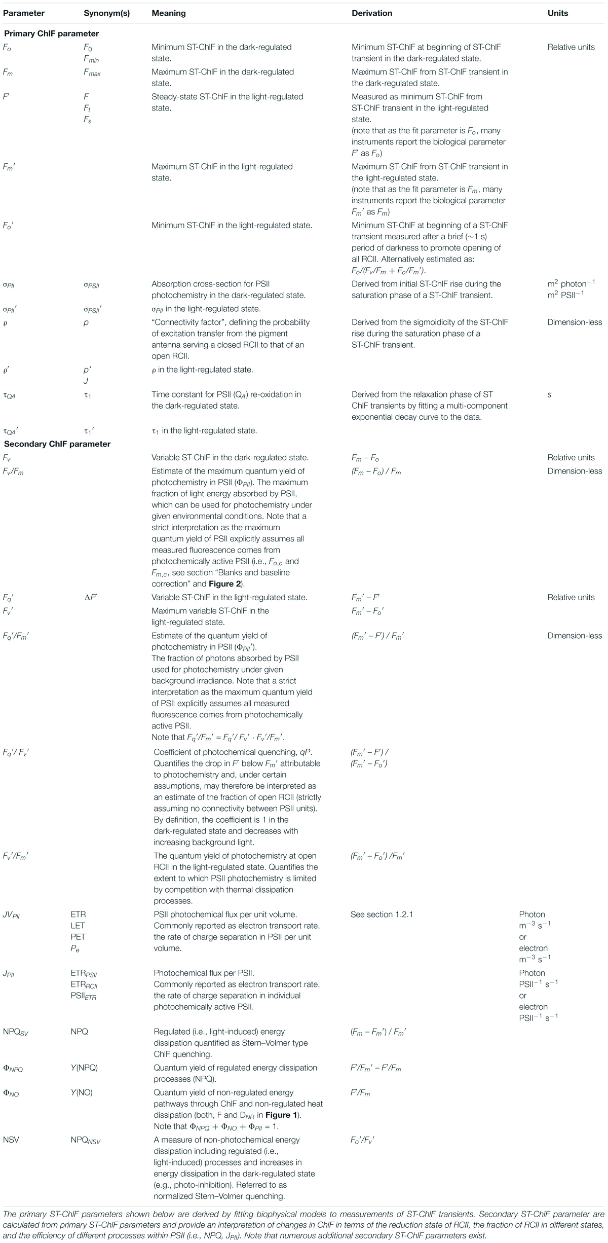
Table 1. Notations and terminology.

Over the past decades, significant progress has been made in the use of ST-ChlF methods in aquatic ecosystems. Developments in sensor technology have greatly improved measurement sensitivity, with current instruments able to collect robust data in the most oligotrophic waters and from autonomous platforms (Lin et al., 2016; Carvalho et al., 2020). At the same time, new approaches to interpret ST-ChlF data in terms of phytoplankton photo-physiology and taxonomic composition allow for a better understanding of the environmental and taxonomic factors driving variability in derived parameters. With maturing technology and a strengthening theoretical framework, ST-ChlF measurements are poised to contribute significant new insights into the variability of phytoplankton photosynthesis over a range of spatial and temporal scales, enabling us to address organismal and ecosystem-level responses to global change. However, the field now sits at a crossroads, as operational, computational, and conceptual approaches to extract and interpret ST-ChlF derived parameters are rapidly diverging. An increasing number of sensors (both commercial and custom-made), sampling protocols, and processing algorithms for ST-ChlF measurements are being developed, yet no standards for best practice have been formally adopted by the international research community. Rapidly growing data sets may thus become increasingly difficult (if not impossible) to reconcile, leading to a “Tower of Babel” scenario, which would limit our ability to build globally coherent ST-ChlF observations and examine large-scale patterns and long-term trends in phytoplankton physiology.

To address the challenges outlined above, SCOR-WG156 was established to assemble minimum standards of best practice for the acquisition and archiving of aquatic ST-ChlF data. Bringing together instrument manufacturers and users from 10 countries and five continents, our group seeks to provide consensus recommendations on the use of ST-ChlF instruments to examine in-situ phytoplankton photo-physiology and productivity. We also seek to broaden the application of ST-ChlF approaches among the aquatic research community, and to support the development of a global synthesis of existing and future data. Importantly, it is not our intention to favor any one particular approach, instrument or conceptual model. Rather, we aim to facilitate the sharing of datasets collected by different researchers and instrument types, establishing protocols to promote inter-comparability of observations at a fundamental level. To this end, our goal is to provide consensus recommendations on instrument deployment, data retrieval, and data archiving. While recognizing that any given scientific application may require context-specific methods and protocols, the generation of a globally consistent data archive would enable researchers to apply existing and emerging approaches of data interpretation, and assess local and global patterns of phytoplankton photo-physiology, photosynthetic rates, and bottom-up controls on primary productivity. Coherent datasets of this kind are invaluable for providing a large-scale and long-term view, and to inform the development of ecosystem models and remote sensing algorithms.

This article represents a collective effort by members of SCOR-WG156 to address key challenges and opportunities for successful global integration of ST-ChlF measurements. We begin with a brief overview of foundational concepts and focus on recommendations toward the acquisition of inter-comparable primary ST-ChlF parameters. We then present a short description of different current approaches to deriving secondary ST-ChlF parameters, emphasizing advantages, and caveats of each approach. In section “Operational and practical considerations” we discuss the need for standards-of-best-practice for field data acquisition. Stressing the importance of data inter-comparability and collaborative community efforts, we also provide recommendations on data reporting and archiving needed to produce globally consistent datasets (section “Data reporting and archiving”). We conclude by discussing the wide scope of potential ST-ChlF applications in the context of phytoplankton primary productivity, community composition, and the refinement of ecosystem models and remote sensing algorithms (section “Integration and application”). Our goal is to highlight key developments in ST-ChlF methodologies, and stimulate broader interest in the application of these powerful approaches to a range of research questions. This discussion forms the starting point of a community-led and evolving Community-Best-Practice document (SCOR Working Group 156, 2021) for, which will provide detailed guidelines and recommendations.

Theoretical Foundations and Concepts

Chlorophyll-a (chla), the primary light-harvesting pigment of photosynthetic organisms, re-emits a fraction of absorbed photons at longer wavelengths as fluorescence (ChlF, e.g., Harbinson and Rosenqvist, 2003). This property provides an optical signal that has been widely used to study photosynthetic organisms under field and laboratory conditions (e.g., Kautsky and Hirsch, 1931; Lichtenthaler, 1988; Papageorgiu and Govindjee, 2004; Suggett et al., 2010a). In aquatic systems, ChlF has long been used to infer total chla concentrations as a proxy for phytoplankton biomass. When measured in-vitro (i.e., after sample extraction in an organic solvent), ChlF is, indeed, proportional to the total chla concentration. However, in-vivo ChlF measurements, such as those derived from chla-fluorometers deployed on depth profiling systems or connected to shipboard continuous flow systems, are subject to variable amounts of so-called “quenching” that cause changes in the ChlF:chla ratio. Quenching mechanisms represent the redirection of variable proportions of the absorbed photons to pathways other than ChlF. The variable ratio between in-vivo ChlF and chla concentration represents an unwanted complication during routine surveys of biomass, necessitating correction procedures (e.g., Thomalla et al., 2018). On the other hand, the variable nature of ChlF provides valuable insights into underlying photo-physiological processes. It is precisely this variability that is examined using variable ChlF methods such as ST-ChlF.

All variable ChlF approaches are based on a fundamental generalized concept, illustrated in Figure 1. Light energy absorbed by the photosynthetic pigments serving PSII follows one of three pathways: (1) photochemistry (P); (2) dissipation as heat (D); or (3) re-emission as fluorescence (F; e.g., Butler, 1978). The distribution of excitation energy among the three pathways is variable. Photochemistry and a component of heat-dissipation (D_NPQ) are actively regulated, and changes in these two processes modulate the remaining fraction of absorbed energy re-emitted as ChlF. When more absorbed light energy is directed to either P or D_NPQ, less energy is re-emitted as ChlF. For this reason, P and the D_NPQ are typically referred to as photochemical and non-photochemical quenching of ChlF, respectively. It follows that changes in ChlF can be used to assess variations in P, as long as changes in D_NPQ can be accounted for. This general concept has been applied and refined for over a century of photosynthetic research (e.g., Govindjee, 1995), leading to many important insights. At the same time, there has been considerable conceptual and methodological confusion associated with varying approaches and nomenclatures employed by different investigators across various photosynthetic taxa and measurement techniques.

FIGURE 1

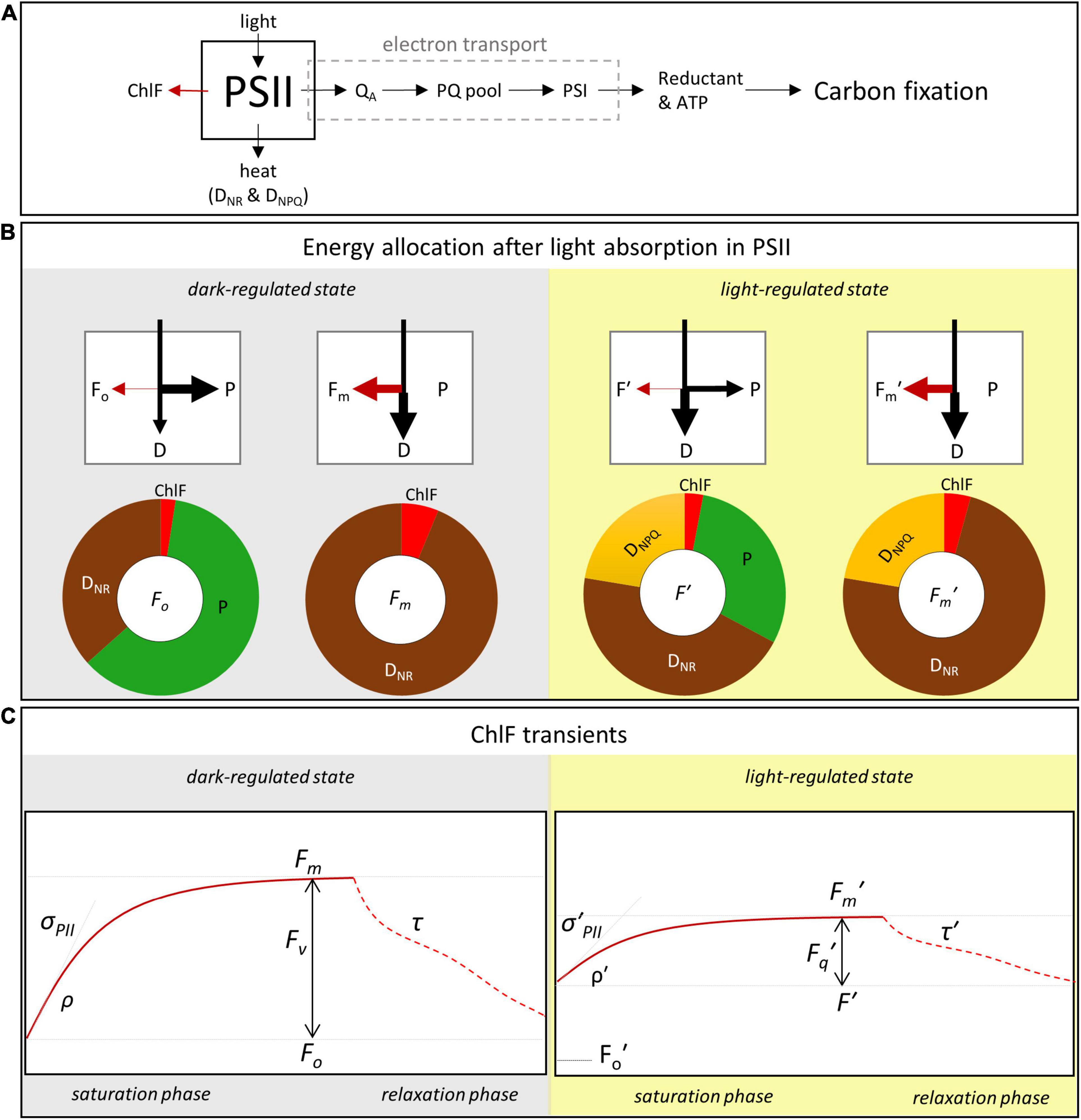
Figure 1. The three energy pathway concept and ChlF transients from typical ST protocols. ChlF induced and detected by ST-ChlF instruments is typically assumed to originate primarily from PSII (A). (B) provides a conceptual overview of energy allocation to the three competing pathways of photochemistry (P), re-emission as heat (D), or ChlF (F). The heat-dissipation pathway is composed of a non-regulated (D_NR) and an actively regulated (D_NPQ) part. Changes in both P and D_NPQ modulate ChlF. During ST-ChlF transients (C), energy allocation to P is selectively modulated, leading to changes in ChlF (see main text). Left hand panels in (B,C) (gray shading) represent the dark-regulated state, while right hand panels (yellow shading) represent the light-regulated state. In the dark-regulated state, it is assumed that D_NPQ is zero, and that all electron transport-chains are fully oxidized at the beginning of the saturation phase (i.e., all RCII are open), leading to the maximum potential for absorbed light energy to be used for photochemistry and thus maximal photochemical quenching of ChlF (ChlF = F_o). During the “saturation phase,” all primary electron acceptors Q_A are progressively reduced (i.e., all RCII are closed, P = 0), thus decreasing photochemical quenching and increasing the energy re-emitted as ChlF (ChlF = F_m). As shown in (C), by fitting the ST-ChlF saturation phase in the dark-regulated state we can derive: minimum (F_o) and maximum (F_m) ChlF, the absorption cross-section for photochemistry (σ_PII), and the connectivity factor (ρ). The decrease of ST-ChlF during the relaxation phase can be interpreted in terms of electron transport rates downstream of charge separation in PSII (τ). In the light-regulated state, the ST-ChlF level at the beginning of saturation phase increases to a steady-state fluorescence, F′. This increase in ChlF reflects the fact that some PSII are engaged in electron transport (Q_A reduced, RCII closed), such that the fraction of absorbed energy potentially allocated to photochemistry is no longer maximal. The maximum ST-ChlF decreases from F_m in the dark-regulated state to F_m′ in the light-regulated state, as a result of ChlF quenching by regulated heat-dissipation pathways (D_NPQ). Further, σ_PII′, ρ′, and τ′ can be derived from the light-regulated ST-ChlF transient. The parameter F_o′ represents the minimum ST-ChlF measured immediately after the transition from light to dark. It is the ST-ChlF level under maximal photochemical quenching (all Q_A oxidized, all RCII open), while D_NPQ is still active at the level induced during the light-regulated state. The conceptual model shown is a simplified and idealized representation and that its applicability to different phytoplankton with a range of photosynthetic architectures and mechanisms will vary.

Numerous books, reviews, and manuals have explained the details of ST-ChlF techniques and the derivation of ChlF parameters (e.g., Roháček and Barták, 1999; Roháček et al., 2008; Huot and Babin, 2010; Kolber, 2021; Oxborough, 2021). Here, we summarize the essentials in Figure 1, and then focus on aspects most relevant to aquatic field deployments of ST-ChlF instruments and the interpretation of the resulting data. In our discussion, we make a distinction between primary ST-ChlF parameters, which are those properties that are directly derived from induced changes in ChlF (ST-ChlF transients), and secondary ST-ChlF parameters, which are subsequently computed from primary ST-ChlF parameters. Importantly, it is not our goal (nor in the interest of scientific progress) to favor any one particular approach for the acquisition or interpretation of ST-ChlF data. Rather, we aim to present foundational concepts and procedures applicable to any hardware and analysis routine, enabling datasets collected by different research groups, instrument types and field campaigns to remain inter-comparable at a fundamental level. Such inter-comparability is needed for the construction of sustainable global datasets and their robust interpretation using existing and emerging approaches.

Primary ChlF Parameters

Variable ChlF approaches use intense light pulses on microsecond timescales to transiently saturate the photochemical pathway, thereby inducing measurable changes in ChlF (Figure 1). Such induced changes in ChlF, referred to as ChlF transients, involve the rapid increase in ChlF up to a maximum value (i.e., the saturation phase), followed by a return to a basal level (i.e., the relaxation phase; Figure 1C). The ChlF signal measured by variable ChlF approaches is assumed to derive exclusively from PSII (but see section “Blanks and baseline correction”). Consequently, the technique is most suited to study reactions and processes taking place at or close to PSII reaction centers II (RCII). However, given tight coupling of reductant and energy fluxes across the entire photosynthetic system and beyond, information well beyond PSII function can be inferred from variable ChlF measurements.

Biophysical models have been developed to interpret ChlF transients and derive primary ChlF parameters (e.g., Dau, 1994; Trissl and Lavergne, 1995). During a saturating single-turnover (ST) flash, light energy sufficient to reduce all primary electron acceptors, Q_A (i.e., to “close” all RCII), is delivered over a short period (<200 μs), before significant electron transport downstream of PSII can re-open RCII (Figure 1A). In contrast, multiple turnover protocols are designed to more gradually reduce the entire electron transport chain over ∼100–1,000 ms, usually leading to higher levels of maximum ChlF (e.g., Kolber et al., 1998; Kromkamp and Forster, 2003; Brown et al., 2019). We focus our discussion here on ST instruments and analysis protocols only, as these are more commonly applied for research on phytoplankton. The rapid reduction of Q_A in ST instruments can be achieved by a series of light “flashlets” in FRRF, or by a single light pulse in fluorescence induction and relaxation (FiRe) and single turnover active fluorometry (STAF) instruments.

Primary ChlF Parameters From the Saturation Phase

In the “dark-regulated” state, measurements are made without any background illumination and after relaxation of any NPQ processes (section “The dark-regulated states and NPQ-relaxation”). Under this condition (left panel in Figures 1B,C), it is assumed that D_NPQ is minimal. All RCII are open at the beginning of the ST-ChlF transient, allowing for a maximum fraction of absorbed photon energy to be partitioned to photochemistry (P is maximal and ChlF minimal). In the dark-regulated state, the amplitude of a ChlF transient (F_v) can be interpreted in terms of the maximum photochemical efficiency for a given population of PSII under a given environmental condition. As described in Figure 1, and in much detail elsewhere (e.g., Kolber et al., 1998; Huot and Babin, 2010), the primary ST-ChlF parameters derived from the saturation phase of dark-regulated ST-ChlF transients are the minimum (F_o) and maximum (F_m) ChlF, the absorption cross-section for PSII photochemistry (σ_PII) and the “connectivity” among PSII units (ρ). F_o and F_m are typically measured in arbitrary units, although they can be calibrated to a reference signal, providing useful additional quantitative information (Oxborough, 2021). Values of σ_PII are derived from the initial ST-ChlF transient rise and are reported in units of area photon^–1 or area PSII^–1. Note that σ_PII has frequently been reported in Ų, but the use of such non-SI units is not recommended. Connectivity among PSII units (ρ) is a unitless value, derived from the sigmoidicity of the ST-ChlF rise from F_o to F_m (Table 1, Lavorel and Joliot, 1972; Lavergne and Trissl, 1995; Kolber et al., 1998).

In the light-regulated state, where the sample is exposed to background illumination during measurements (right panel in Figures 1B,C), a fraction of the RCII pool is already closed at the beginning of the ST-ChlF transient. As a result, the minimum ChlF level derived from the ChlF transient (F′) is generally increased relative to the minimum ChlF for fully open RCII (F_o). Depending on the intensity and duration of the background irradiance, the fraction of absorbed photon energy dissipated as heat may be increased relative to the dark-regulated state, resulting in a drop (i.e., quenching) of ChlF (F_m′ < F_m, F_o′ < F_o, see section “Non-photochemical quenching”). As described in Figure 1, the primary ST-ChlF parameters derived from the saturation phase in the light-regulated state are F′, F_m′, σ_PII′, and ρ′. We note here that, in contrast to higher plants and green algae, the light-dependent decrease in F_m′ relative to F_m in many phytoplankton samples is frequently preceded by a transient increase in F_m′ upon moderate illumination (e.g., Gorbunov et al., 2011). The underlying causes of such transient increases in F_m′ are still debated, and readers are referred to SCOR Working Group 156 (2021) for a more detailed discussion of this phenomenon.

Primary ST-ChlF Parameters Derived From the Relaxation Phase

Following the transient closure of RCII during the saturation phase, ChlF decreases back to its minimal level (Figure 1C). The time-course of this ChlF decrease largely reflects Q_A re-oxidation kinetics through downstream photosynthetic electron transport (Figure 1A). With the FRRF method, this ST-ChlF “relaxation phase” is typically resolved through a series of low frequency “probing flashlets” often applied at gradually increasing intervals (Kolber et al., 1998). An alternative approach is to apply a small number of more widely spaced ST saturation phases. A “multi-flash” (comprising five ST saturation phases) protocol, with an increasing interval between adjacent ST phases was implemented in a single-cell FRRF (Gorbunov et al., 1999). A “dual-pulse” protocol with a variable gap between two ST saturating phases has been incorporated within “single-turnover active fluorescence” (STAF) instruments (Oxborough, 2021). In all cases, the time-dependent decrease in ChlF after saturation is fit to a multi-component exponential decay curve to resolve the time constant(s; τ) for Q_A re-oxidation (Kolber et al., 1998; Gorbunov and Falkowski, 2020; Oxborough, 2021, Figure 1). The use of a three-component kinetic analysis is critical for the most accurate description of Q_A re-oxidation kinetics (Gorbunov and Falkowski, 2020). However, the fitting of three (or more) components requires a high signal-to-noise ratio, which is not always achievable in oligotrophic regions or with older and less sensitive instrument types.

Uncertainty and Error

Multiple factors can limit the accuracy with which primary ST-ChlF parameters can be retrieved. However, despite previous attempts to draw attention to some of these issues in specific instruments (e.g., Laney, 2003; Laney and Letelier, 2008), uncertainty and error associated with primary ST-ChlF parameters are not routinely described in the literature, nor reported in published datasets. This limits our ability to gage data quality, and the strength of any derived observations and interpretations. To address this limitation, we outline several considerations specific to the derivation and reporting of primary ChlF parameters. While the exact approach may be instrument specific, an explicit consideration of data quality and confidence is nonetheless critical to support globally coherent and inter-comparable observations.

Single-turnover variable chlorophyll fluorescence instruments are now capable of acquiring data even in very low biomass regions, but the low signal typical for oligotrophic waters often requires considerable data averaging from repeated rounds of ST-ChlF transients to achieve fits of reasonable quality (e.g., Ryan-Keogh and Robinson, 2021). A minimum level of fit quality for the derivation of primary ST-ChlF parameters should preferably be assessed during real-time data acquisition. Using this information, appropriate instrument settings and signal averaging can ensure minimum data quality standards. In addition to measurements taken in oligotrophic waters, the assessment of quality of ST-ChlF transient fits is particularly important for measurements taken at high background light levels, where the amplitude of the ST-ChlF transient decreases and retrieved parameters, σ_PII′ and τ′ in particular, become imprecise. As discussed in section “Data reporting and archiving,” information regarding the statistical goodness of the fit of ST-ChlF transients should be archived alongside primary ST-ChlF parameter data.

In addition to the general statistical issues described above, other factors need to be considered in the derivation of individual primary ST-ChlF parameters. For example, both F_m(′) and σ_PII(′) rely, in principle, upon closure of all RCII on time-scales shorter than RCII reopening (<200 μs), which results in a clear plateau of the ST-ChlF transient toward the end of the saturation phase (Figure 1C). On a practical level, this requirement is generally easily achieved when ChlF is excited in the 410–500 nm spectral range, which is strongly absorbed by most eukaryotic phytoplankton species, and for which LEDs with high photon flux are readily available. However, when excitation power is delivered at wavelengths poorly absorbed by the present phytoplankton taxa, or at wavelengths served by less effective LEDs, the photon flux achievable during the short ST saturation phase may be insufficient for near complete Q_A reduction. Such “under-saturation” of the ChlF transient is taken into account during data fitting (Kolber et al., 1998), but very low (50%) saturation combined with a low signal-to-noise ratio, can make it challenging to derive accurate primary ST-ChlF parameters. Given these challenges, users should confirm sufficient Q_A reduction (ST-ChlF transient saturation) in their measurements (Table 2).

TABLE 2

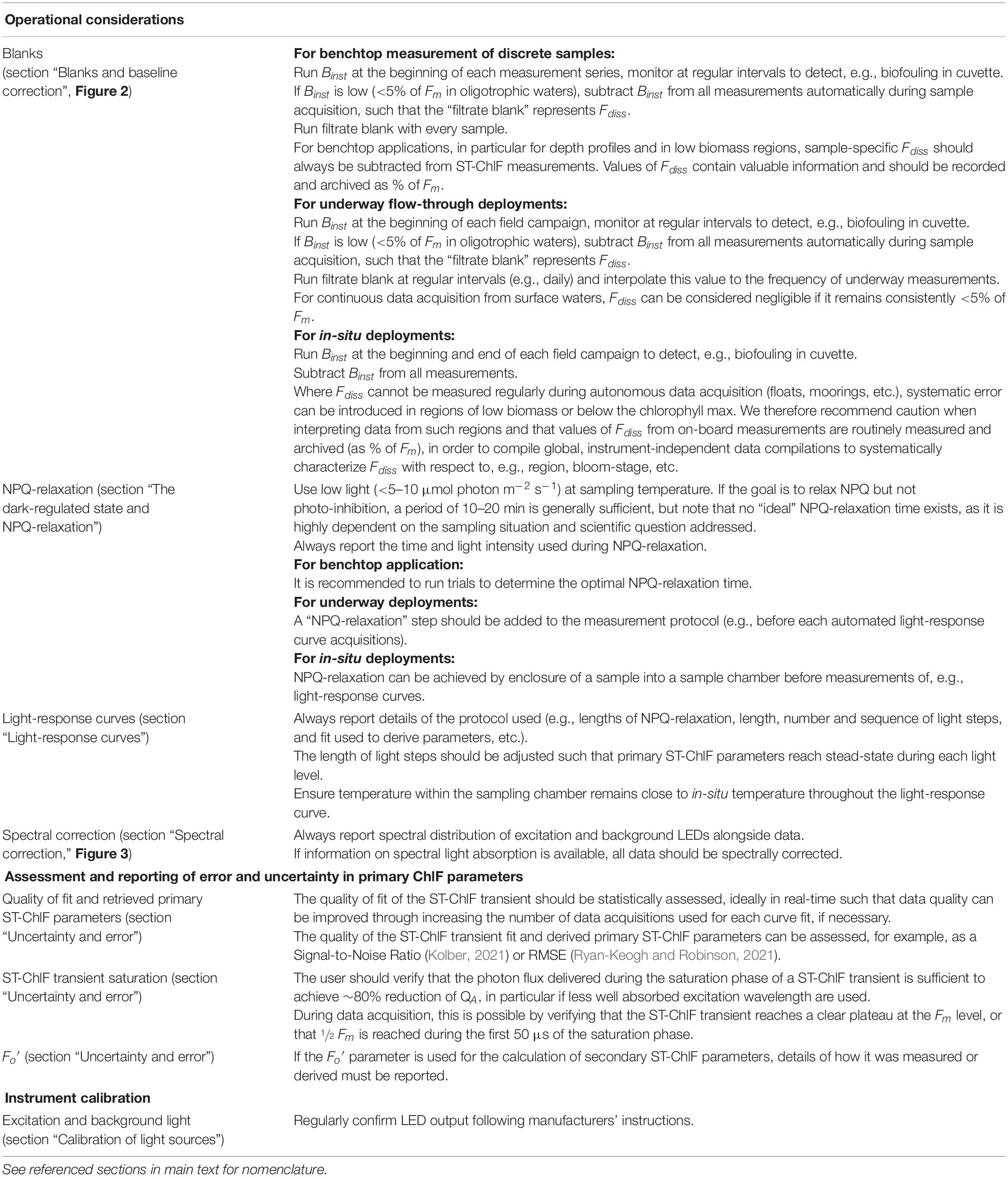
Table 2. Consensus recommendations for the field deployment of ST-ChlF instruments, aimed at supporting the development a globally coherence ST-ChlF dataset.

Special considerations are required for the light-regulated ChlF parameter F_o′. This parameter represents the minimum ChlF expected when the photochemical potential is maximal (i.e., all photochemically active RCII in the open state), but with light-dependent regulation of the heat dissipation pathway (D_NPQ) still active (e.g., Genty et al., 1989). In principle, F_o′ can be measured by acquiring a ST-ChlF transient immediately after turning off the background light, under the assumption that re-oxidation of the electron transport chain will occur on time-scales much shorter than those required for the relaxation of NPQ (Ni et al., 2017). In practice, some NPQ processes may begin relaxing on very short timescales (Roháček et al., 2014; Ni et al., 2017). Measuring an accurate F_o′ thus becomes problematic, particularly in low biomass regions where averaging of many sequential ChlF transients may be necessary to obtain good quality data. In a second approach, introduced by Oxborough and Baker (1997), F_o′ is estimated as F_o′ = F_o/(F_v/F_m+F_o/F_m′). The derivation is based on the widely accepted concept of competing energy pathways in PSII, but is susceptible to distortion by baseline fluorescence (section “Blanks and baseline correction”) and relies on measurements in the dark regulated state (section “The dark-regulated states and NPQ-relaxation”). As discussed in section “PSII photochemical flux, J_PII,” incorrect values for F_o′ can introduce systematic error in the derivation of some secondary ST-ChlF parameters.

In addition to the sources of error and uncertainty described above, other sources of variability in the derivation and interpretation of primary ST-ChlF parameters include uncertainty in conceptual models assessing connectivity between PSII units (ρ; e.g., Stirbet, 2013; Oxborough, 2021); the appropriate number of exponential decay lifetimes (τ) used to model the relaxation of ST-ChlF (e.g., Gorbunov and Falkowski, 2020) and the effects of carotenoid quenching on$F_m({}^{\prime })$ (e.g., Kolber et al., 1998; Schreiber et al., 2019). Specific details of these effects are beyond the scope of this article, but readers are referred to SCOR Working Group 156 (2021) for further details.

Finally, it is important to highlight taxonomic diversity as a factor that complicates the derivation and interpretation of primary ST-ChlF parameters from models developed for homogeneous populations of PSII. For example, values of σ_PII measured on mixed phytoplankton assemblages are unlikely to scale linearly with the proportional contributions of σ_PII from the individual species present (Suggett et al., 2004; Laney, 2010). In addition, taxonomic variability in baseline fluorescence levels (see section “Blanks and baseline correction”) has the potential to significantly increase non-variable ChlF, and disproportionately increase apparent minimum (F_o or F′) relative to maximum (F_m or F_m′) ChlF. For example, fluorescence from phycobilins can be falsely attributed to PSII, and such contributions can vary significantly between dark and light-regulated states. It has furthermore been shown that taxonomic trends in PSII:PSI ratios can lead to differential contributions of PSI-derived ChlF to signals usually interpreted in terms of PSII (Campbell et al., 1998). Such taxonomic influences, and other sources of baseline fluorescence not emanating from the PSII pigment pool, will complicate the physiological interpretation of widely used primary and secondary ST-ChlF parameters (section “Blanks and baseline correction”).

Secondary ST-ChlF Parameters

The primary ST-ChlF parameters described above are those derived directly from applying photo-physiological models to ST ChlF transients (Figure 1). These primary parameters can, in turn, be used to derive secondary parameters of physiological interest (Table 1). Here, we focus on J_PII and NPQ, reviewing the most common algorithms used to estimate these parameters and describing their respective advantages and disadvantages with respect to field data. In this discussion, it is important to understand that secondary ST-ChlF parameters such as J_PII are not directly measured, but rather derived from primary ST-ChlF parameters using conceptual models based on current understanding of the photosynthetic process. Under field conditions, where taxonomic and environmental variability are the norm, the applicability of different models to derive J_PII (and other secondary ST-ChlF parameters) may vary, and results could diverge. While this can create uncertainty, the goal here is not necessarily to identify one “correct” approach, but rather to understand how and why different models may differentially capture underlying physiological processes under various conditions (Table 3). The compilation of globally consistent and inter-comparable primary ST-ChlF parameter data will greatly facilitate the comparisons of different models to derive J_PII (and other parameters). Important insights will likely be found in situations where results from different modeling approaches diverge.

TABLE 3

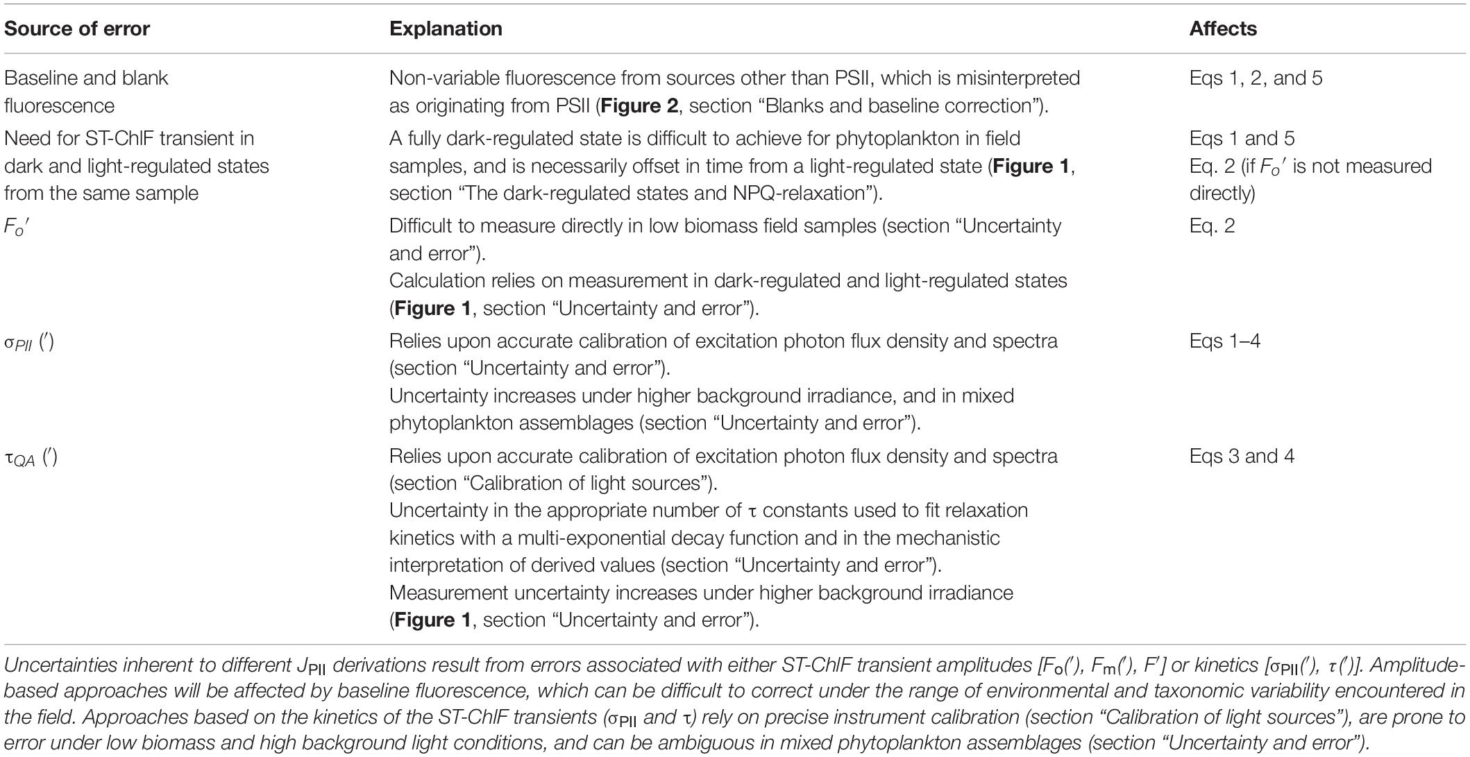
Table 3. Sources of error in different J_PII estimates.

PSII Photochemical Flux, J_PII

Primary ST-ChlF parameters can be used to quantify the photochemical pathway (Figure 1) in terms of the PSII photochemical flux. We use the term PSII photochemical flux (J_PII) rather than the commonly used term electron transport rate to emphasize that the parameter quantifies the flux of solar photons toward metabolically useful biochemical energy in the form of redox potential in the photosynthetic electron transport chain at the level of PSII. Units of J_PII are (absorbed) photon PSII^–1 s^–1. However, given that each photon absorbed and delivered to RCII leads to one charge separation, the parameter is widely reported in units of electrons PSII^–1 s^–1. A proportion of the biochemical energy available through J_PII is ultimately captured in the form of reduced organic carbon, and it is this connection to carbon-based primary productivity that often motivates the measurement of J_PII in aquatic environments (section “Deriving carbon-based primary productivity,” Hughes et al., 2018).

Equations 1 and 2 show different versions of the so-called “sigma-algorithm,” commonly used to derive J_PII in aquatic systems. Both equations follow the simple rational that J_PII can be calculated from estimates of incident photon irradiance, the fraction of photons absorbed by PSII and the distribution of absorbed photon energy among the three energy dissipation pathways (Figure 1). Equations 1 and 2 are algebraically equivalent, but differ operationally in their approach to estimating light-dependent changes in absorbed energy allocation among the three pathways (e.g., Gorbunov et al., 2001; Suggett et al., 2010b). In Eq. 1, light absorption of PSII-associated pigments specific to all three pathways is estimated as the product of scalar irradiance (E), σ_PII and (F_v/F_m)^–1. This estimate of light absorption is then multiplied by the quantum efficiency of photochemistry (i.e., changes in the distribution of energy between the three pathways) under a given background light intensity, F_q′/F_m′.

$J_{\text{PII}}=E\cdot {\mathrm{\sigma }}_{\text{PII}}\cdot {(F_v/F_m)}^{-1}\cdot ({\mathit{F}}_q{}^{\prime }/{\mathit{F}}_m{}^{\prime })(1)$

In Eq. 2, light absorption directed to the photochemical pathway at a given irradiance only is quantified as the product of E and σ_PII′. The parameter F_q′/F_v′, calculated as (F_m′-F′)/(F_m′-F_o′), is used as an estimate of the fraction of RCII in the open state (Table 1, Kolber et al., 1998; Kramer et al., 2004).

$J_{\text{PII}}=E\cdot {\mathrm{\sigma }}_{\text{PII}}^{\prime }\cdot (F_q^{\prime }/F_v^{\prime })(2)$

Equations 1 and 2 are equivalent when the ratio of light to dark regulated absorption cross-section of PSII photochemistry, σ_PII’/σ_PII, is equal to the ratio of light to dark regulated quantum yield of photochemistry, (F_v′/F_m′)/(F_v/F_m); (Gorbunov et al., 2001; Suggett et al., 2010b).

The approach represented by Eqs 1 and 2 has several limitations (Table 3). First, it relies on the measurement of ST-ChlF amplitudes (i.e., changing levels of fluorescence, F), which can be affected by baseline fluorescence (section “Blanks and baseline correction”), although this has a larger influence on Eq. 1 than Eq. 2. Further, Eq. 1 requires measurements from separate ST-ChlF transients offset in time (dark- and light-regulated state), and the need to achieve a fully dark-regulated state, which can be challenging under field conditions (section “The dark-regulated states and NPQ-relaxation”). For Eq. 2, measurements in the fully dark-regulated state are required if the F_o′ value needed to calculate F_v′ is derived following the approach by Oxborough and Baker (1997; section “Uncertainty and error”). To address these challenges, Eq. 3 has been proposed as an alternative to Eq. 2:

$J_{\text{PII}}=E\cdot {\mathrm{\sigma }}_{\text{PSII}}^{\prime }\cdot [1/(1+({\mathrm{\sigma }}_{\text{PSII}}^{\prime }\cdot E\cdot {\mathrm{\tau }}^{\prime }))](3)$

Here, the calculation of the fraction of RCII in the open state (in square brackets) uses a mechanistic model depending on σ_PII′ (energy distributed to the photochemical pathway, i.e., closing RCII) and 1/τ′ (rate of re-opening of RCII). All parameters used in Eq. 3 can be derived from a single saturation/relaxation profile measured in the light-regulated state.

Recently, Gorbunov and Falkowski (2020) introduced an approach for the estimation of J_PII which relies almost exclusively on the kinetics of the relaxation phase of the ST-ChlF transient.

$J_{\text{PII}}=1/\mathrm{\tau }\cdot [(E\cdot \frac{F_q^{\prime }}{F_m^{\prime }})/(E_{\text{max}}\cdot {\frac{F_q^{\prime }}{F_m^{\prime }}}_{(E_{\text{max}})})](4)$

As explained in more detail in Gorbunov and Falkowski (2020), J_PII in this approach is derived from the time constant of Q_A re-oxidation, τ_QA′, derived from the first of a three-component decay function fit to the relaxation phase of a ST-ChlF transient (section “Primary ST-ChlF parameters derived from the relaxation phase”), at saturating background light. τ_QA′ was confirmed in independent experiments to closely approximate the maximum rate (P_max) of short-term ¹⁴C-uptake (here referred to as the photosynthetic turnover rate, τ). The second term (in square brackets) of Eq. 4 characterizes the shape of a light response curve, and thus scales the maximum J_PII to light availability. In Eq. 4, E_max is taken as a value three time higher than the light saturation parameter, E_k.

All of the approaches described above estimate PSII photochemical flux per photochemically active PSII (J_PII, photon PSII^–1 s^–1 or electron PSII^–1 s^–1). In order to derive a volume-specific PSII photochemical flux (JV_PII, photons m^–3 s^–1 or electron m^–3 s^–1), information is required on the concentration of functional PSII. This can be done either directly on a volumetric basis ([PSII] m^–3), or indirectly through a normalization to chla concentrations ([PSII] chla^–1; n_PSII) and determination of [chla]. Different approaches to quantify [PSII] or n_PSII exist (see, e.g., Silsbe et al., 2015), but none of these are practical for high-resolution autonomous field measurements. At the same time, the use of an assumed constant value for n_PSII can result in considerable error. Consequently, Oxborough et al. (2012) have developed an approach, subsequently verified by Silsbe et al. (2015) and extended by Boatman et al. (2019), to estimate [PSII] from ST-ChlF measurements. In simple terms, the approach recognizes that values of F_o should scale with the number of active PSII within a sample, while σ_PII provides a measure of the size of a single PSII. From this it follows that the number of PSII within a sample can be estimated by using an appropriate instrument-specific scaling factor, K_a (m^–1), such that [PSII] = F_o/σ_PII ⋅ K_a. Incorporation of [PSII] into the J_PII-algorithm shown in Eq. 1 provides the means to calculate JV_PII, where the term in square brackets estimates light absorption by all PSII within a volume of water (a_LHII, m^–1) and F_q′/F_m′ represents the efficiency with which this energy is used for photochemistry (Oxborough, 2021).

$J{V}_{\text{PII}}=E\cdot F_q^{\prime }/F_m^{\prime }\cdot [K_a\cdot (F_m\cdot F_o)/F_v](5)$

This approach, referred to as the “absorption algorithm” enables the calculation of volume-specific, rather than PSII-specific photochemical fluxes, and thus represents an important step forward in our ability to quantify phytoplankton primary productivity from ST-ChlF measurements. Importantly, it allows the quantification of light absorbed by all PSII within a volume of water (a_LHII, m^–1), and does not rely on estimates of absorption cross-sections for PSII photochemistry (σ_PII), which are ambiguous in heterogeneous populations of PSII and therefore difficult to interpret in mixed phytoplankton assemblages in the field. However, as with any amplitude-based technique, estimates of [PSII] and the associated absorption algorithm are prone to error introduced by baseline fluorescence (section “Blanks and baseline correction”) and requires measurements in a fully dark-regulated state (section “The dark-regulated states and NPQ-relaxation”). Furthermore, the effect of reabsorption of ChlF in large or highly pigmented cells (“pigment packaging”) must also be considered (Boatman et al., 2019), and the approach relies on precise calibration of the absolute ChlF yields through procedures not routinely applied for all instrument types. The application of the absorption algorithm to a wide range of environmental conditions and phytoplankton taxa will allow to determine how the necessary corrections can be confidently and routinely applied.

Non-Photochemical Quenching

All plants and most algae possess a range of mechanisms that can be rapidly activated to dissipate potentially harmful excess excitation energy in the pigment antenna under conditions of transient increases in incident light. Collectively these are known as non-photochemical quenching (NPQ) mechanisms, due to their ability to physiologically quench excitation energy. As described above, activation of NPQ will lead to a decrease in ChlF, such that different metrics of NPQ can be derived from ST-ChlF measurements. In this respect, “NPQ” describes the phenomenon of non-photochemical quenching of ChlF rather than excitation energy. The effect of NPQ on ChlF complicates the interpretation of ChlF as a biomass proxy and the interpretation of ST-ChlF measurements in terms of photochemistry. On the other hand, NPQ holds untapped potential as an optical signal reflecting the physiological state of phytoplankton (Campbell et al., 1998; Schuback et al., 2020; section “Exploring environmental controls on primary productivity”), which can, in turn, constrain key parameters for estimating productivity (Schuback et al., 2015).

Current definitions and terminologies for NPQ are particularly confusing, with the existing literature and assumptions derived primarily from higher plant research. As we are only beginning to understand the diversity of NPQ mechanisms and capabilities across different phytoplankton species (e.g., Goss and Lepetit, 2015; Magdaong and Blankenship, 2018; Lacour et al., 2020), great caution should be taken when interpreting patterns of different NPQ metrics in phytoplankton based on models or mechanisms extrapolated from higher plants.

Multiple metrics of NPQ can be derived from ST-ChlF measurements. Most commonly, NPQ is quantified according to Stern–Volmer quenching principles (NPQ_SV, Eq. 6), as the difference in maximum ChlF between the dark-regulated (F_m) and light-regulated state (F_m′; see also Figure 1).

${\text{NPQ}}_{\text{SV}}=(F_m-F_m^{\prime })/F_m^{\prime }(6)$

NPQ_SV, which was first introduced by Bilger and Björkman (1991), provides a mechanistic metric tracking the accumulation of a ChlF quencher within a sample exposed to increasing photon flux. It is an unbound parameter, with values above ∼2 showing poor correlation with other photo-physiological metrics of excitation dissipation (e.g., Xu et al., 2018).

The parameter F_v′/F_m′ arguably most closely tracks the impact of NPQ on PSII photochemical efficiency under different conditions.

$F_v^{\prime }/F_m^{\prime }=(F_m^{\prime }-F_o^{\prime })/F_m^{\prime }(7)$

A different approach can be used to derive the fractional yields of regulated NPQ (Φ_NPQ, Eq. 8) and non-regulated energy dissipation processes (Φ_NO, including both un-regulated energy re-emission as heat and ChlF, Table 1) akin to the yield of photochemistry (F_q′/F_m′ = Φ_PSII, Table 1), such that Φ_NPQ+Φ_NO Φ_PSII = 1 (Table 1, Hendrickson et al., 2004; Kramer et al., 2004; Klughammer and Schreiber, 2008), where:

${\mathrm{\Phi }}_{\text{NPQ}}=F{}^{\prime }/F_m{}^{\prime }-F{}^{\prime }/F_m(8)$

More recently, the so called normalized Stern–Volmer quenching metric (NSV, Eq. 9), has been applied to aquatic ST-ChlF measurements (McKew et al., 2013; Oxborough, 2021).

$\text{NSV}=F_o^{\prime }/F_v^{\prime }(9)$

In this approach, changes in the heat dissipation pathway in both the dark and light-regulated state (D_NPQ and D_NR in Figure 1) are considered, which is useful in comparing samples acclimated to different light intensities or nutrient regimes.

All the above metrics of NPQ can be affected by baseline fluorescence (section “Blanks and baseline correction”), and it is worth pointing out that an observed decrease in F_m to F_m′ can be caused irrespective of a change in the concentration of a quencher (e.g., state transition, Krause and Weis, 1991). Notwithstanding the different metrics used to quantify NPQ, current ST-ChlF instruments enable us to link our understanding of the physiological processes of NPQ in phytoplankton across molecular and eco-physiological levels. Controlled single-species laboratory experiments will provide additional insight into the photo-physiological plasticity underlying phytoplankton regulation of photosynthesis and photo-protection. At the same time, globally consistent and inter-comparable datasets of primary ST-ChlF parameters will reveal patterns in NPQ across ecologically relevant scales. Temporal or spatial patterns in photo-protection, observed through apparent variability in NPQ, could provide an optical proxy of nutrient limitation – a major determinant of aquatic productivity. Intriguingly, large scale patterns of NPQ proxies can also be obtained from (existing archives of) in-vivo ChlF measurements (section “Exploring environmental controls on primary productivity”), and potentially from changes in spectral absorption indices detectable by remote sensing approaches (Méléder et al., 2018). A foundational understanding of NPQ mechanisms, which can be advanced by careful deployment of ST-ChlF instruments, will help to advance these high-level objectives.

Operational and Practical Considerations

The conceptual foundations described above provide the basis for interpreting variable ChlF data. In practice, a range of operational factors can significantly influence the quality and interpretability of observations, particularly during field deployments. We briefly discuss several important aspects below and refer readers to SCOR Working Group 156 (2021) for more detailed information.

A range of options are available for field deployment of ST-ChlF instruments, each with their own strengths and challenges. In ship-board laboratories, discrete samples can be analyzed individually, or data can be continuously acquired from a flow-through seawater supply (e.g., Behrenfeld et al., 2006). Truly in-situ data acquisition can also be achieved using instruments deployed on depth-profiling packages, towed platforms (e.g., Moore et al., 2003) or autonomous platforms, including moorings, floats, and gliders (e.g., Fujiki et al., 2008; Carvalho et al., 2020). Whereas continuous data collection provides advantages of high frequency measurement, discrete analysis allows for better control and optimization of experimental protocols for individual samples (e.g., light-response curves, NPQ-relaxation, tuning of ST protocols, and blank correction). For all deployment approaches, it is important to systematically identify the key operational factors with the greatest effect on ST-ChlF measurements, and to provide practical guidance on how these might be controlled and quantified (see also Laney, 2010). In the following, we focus our discussion on those operational aspects that should most influence the inter-comparability of ST-ChlF data from different researchers and instrument types. It is important to emphasize that no single approach will be optimal for all research needs across all systems. Rather, the goal is to understand and document the effects of different operational decisions on the resulting measurements.

Instrument Calibration and Standards

Calibration of ST-ChlF instruments is fundamental to ensure the collection of accurate and inter-comparable data by the global user community. The need for robust calibration approaches is particularly important given the increasing availability of custom-made instruments (e.g., Fujiki et al., 2008; Hoadley and Warner, 2017), for which data quality targets need to be defined. A comprehensive discussion of instrument calibration, taking into account particularities of specific instruments, will be provided in the Community-Best-Practice document (SCOR Working Group 156, 2021).

Calibration of Light Sources

Two categories of light sources are used in ST-ChlF instruments. In all instruments, strong “excitation light” is used to induce ST-ChlF transients. In addition, within many instruments, background (“actinic”) light is used to drive variable rates of photochemistry during light-regulated states (e.g., during light-response curves). The LEDs used as light sources in current instruments are typically very stable. Nonetheless, users should be aware of the need for routine monitoring and calibration of the photon flux density of these light sources to ensure quality and consistency of produced data. In the case of excitation light, proper calibration is crucial for the derivation of σ_PII in absolute units and, by extension, derivation of J_PII (section “PSII photochemical flux, J_PII′’) using equations that involve σ_PII. Calibration of the background light is also important for robust data interpretation, for example to obtain inter-comparable values of light-response curve fit parameters (α and E_k; see section “Light-response curves”). Finally, as discussed further in section “Spectral correction,” it is important to characterize and document the spectral quality of light provided by both excitation and background light, since LED spectra can vary significantly even from unit to unit within a manufacturing run.

At present, most end-users are not aware of the importance and difficulty of accurate light source calibration, and no standard protocols or procedures exist. The stability of LED light sources means that factory calibrations can remain valid for periods of months to years, but methods for “in-field” verification would clearly be desirable. Hand-held PAR sensors can be used to measure incident light fields within the sampling cuvette, but these calibrations can be rather finicky, sometimes pushing PAR sensors past their limits of dynamic range and response times. A major design challenge is achieving even illumination of all phytoplankton cells within the detected volume of the instrument. Going forward, we recommend that commercial instrument manufacturers provide guidelines, and perhaps ancillary hardware (e.g., cuvette inserts for light meter probes), for routine light source calibration.

Blanks and Baseline Correction

As described in section “Theoretical foundations and concepts,” measurements of ST-ChlF transients are used to quantify the variable ChlF between a minimum (F_o or F′) and maximum (F_m or F_m′) value. This variable ChlF is superimposed on a non-inducible (i.e., invariant) background fluorescence signal, which includes both a non-physiological component, the analytical blank, and a physiological component, the non-variable baseline fluorescence (Figure 2). The analytical blank represents background instrument noise (B_inst), and fluorescence originating from the dissolved phase of a sample (F_diss). The analytical blank can be significant relative to the measured values in oligotrophic regions (Cullen and Davis, 2003; Moore et al., 2008), and correction procedures are thus important. The baseline fluorescence is a physiological signal, often interpreted in the context of nutrient limitation (Behrenfeld et al., 2006; Macey et al., 2014), but not always fully characterized or understood. While baseline ChlF is not an operational issue, per se, we discuss it together with the analytical blank, as understanding the different sources of non-inducible fluorescence is crucial for correct data interpretation. The prevalence of baseline fluorescence, in particular in phytoplankton compared to higher plants, and the uncertainty around the sources and correct interpretation of this signal has contributed to confusion surrounding the application of ST-ChlF instruments in aquatic environments.

FIGURE 2

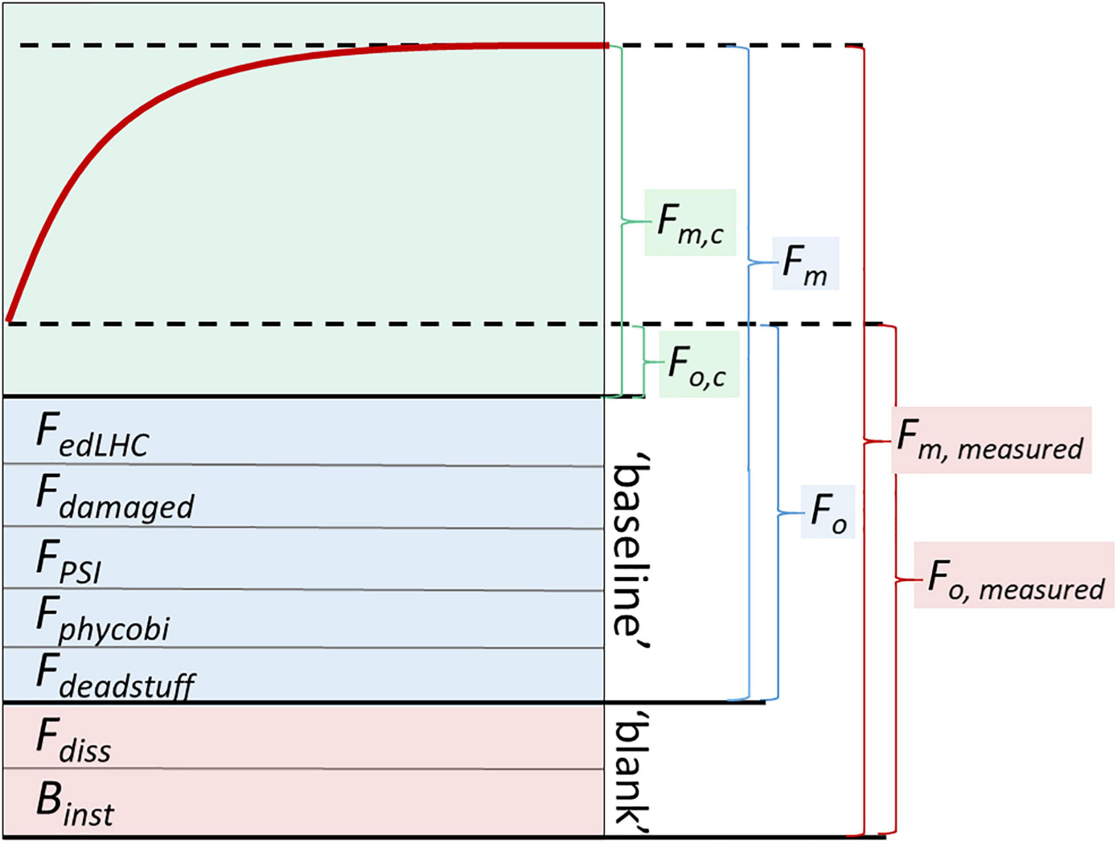
Figure 2. Conceptual diagram of the components of the ChlF signal. The top part of the figure (green shading) shows a hypothetical ST-ChlF transient with ChlF from photochemically active PSII increasing from minimum (F_o,c) to maximum (F_m,c) values. This physiological signal is superimposed on several additional sources of non-inducible fluorescence. The analytical blank (pink shading) generally consists of instrument-specific blank (B_inst) and fluorescence from dissolved fluorophores in the sample (F_diss). Operationally, the analytical blank is defined as the apparent ChlF signal recorded in a 0.2 μm filtrate. B_inst largely reflects optical cross-talk between the instrument excitation and emission channels and can be operationally determined through measurement of ultra-pure water. The baseline fluorescence (blue shading) is composed of F_deadstuff (non-living but still fluorescent phytoplankton and associated detritus), and a number of fluorescence sources in living phytoplankton. These latter sources include contributions from phycobiliproteins in some taxa (collectively F_phycobi), and fluorescence from PSI (F_PSI), which is not always negligible. Non-inducible fluorescence can also originate from damaged or inactive PSII complexes (F_damaged) or energetically decoupled light harvesting complexes (F_edLHC). Well-established correction procedures for baseline fluorescence do not exist, such that the interpretation of secondary ST-ChlF parameters based on models which explicitly assume ChlF to be specific to photochemically active PSII need to be treated with caution, particularly in phytoplankton assemblages in the field, where baseline fluorescence can be substantial. Conventionally, blank-corrected minimum and maximum ST-ChlF values, or values for which the blank was considered negligible, are reported as F_o and F_m in the literature, while baseline-corrected values have been referred to as F_o,c and F_m,c. Note that the contributions of non-inducible fluorescence components in this conceptual diagram are not to scale, and would vary in amplitude in natural samples.

As shown in Figure 2, changes in the non-variable background fluorescence signal will affect F_o proportionally more than F_m, thereby affecting derived secondary ST-ChlF parameters (i.e., resulting in a drop in derived F_v/F_m). Consequently, correction is needed to collect the highest quality data possible (Table 2). Here, we separate the analytical blank into two components, B_inst and F_diss, both of which should be monitored regularly during field deployments of ST-ChlF instruments. For example, routine monitoring of B_inst (derived from measurements of ultra-pure water) is important to verify the absence of fouling in the sampling cuvette. Values of B_inst, originating from background luminescence of optical components (lenses, filters, and optical windows) induced by direct or elastically scattered excitation light can vary significantly between instrument types. Much progress has been made in lowering B_inst in newer instruments, resulting in blank (=B_inst + F_diss) values consistently <5% of F_m values even in the most oligotrophic open ocean waters. For such low B_inst values, it may be acceptable to subtract a constant B_inst from all measurements. Higher B_inst values may be difficult to correct because the amount of scattered excitation light inevitably varies among samples and will, for example, increase dramatically when highly scattering cells (e.g., calcified coccolithophores or chain-forming diatoms) are present in the sample.

Non-inducible fluorescence in the dissolved phase, F_diss, can be of particular importance in low biomass regions, and at depths below the chlorophyll maximum, where high background values can cause significant systematic error in the interpretation of F_v/F_m. During some deployments (e.g., unattended ship-board operation or extended in-situ deployments), routine F_diss correction can be challenging. Under such conditions, particularly for measurements in high biomass surface regions where the value of F_diss is frequently negligible relative to ChlF, it may be sufficient to subtract an instrument and wavelength-specific B_inst value from all measurements. Where there is a need to conduct regular F_diss measurements, it should be possible to develop simple fluidic systems to periodically introduce filtered water into the measurement chamber using automated micropumps and valves.

In contrast to the analytical blank, variations in baseline fluorescence can be rather complex, reflecting differences in the taxonomic composition and physiological state of phytoplankton assemblages. It is crucial to understand and resolve this term for correct interpretation of ST-ChlF data, as the models used for their interpretation explicitly assume that all measured ChlF is specific to the pigment pool of active PSII (F_o,_c and F_m,c in Figure 2). Therefore, correction for baseline fluorescence is necessary for a strict interpretation of F_v/F_m as the quantum yield of photochemistry in PSII and when calculating [PSII] or JV_PII following the absorption algorithm of Oxborough et al. (2012) and Boatman et al. (2019), or J_PII using Eqs 1, 2.

Low measured F_v/F_m values, not corrected for baseline fluorescence, are well established as an indicator of iron limitation and have been explained by the presence of energetically-decoupled light harvesting complexes (edLHC), which absorb light and emit ChlF, but do not transfer energy toward photochemistry (e.g., Behrenfeld and Milligan, 2013; Macey et al., 2014). These complexes contribute to the baseline fluorescence signal and thus increase the measured values of F_o and F_m by equal amounts, leaving F_v unchanged and hence lowering F_v/F_m. A decrease in F_v/F_m due to increased baseline fluorescence can also result from processes other than F_edLHC (Figure 2). However, limitation by nutrients other than iron does not always result in decreased F_v/F_m (e.g., Parkhill et al., 2001; Kruskopf and Flynn, 2006), likely because only severe starvation would lead to an accumulation of damaged PSII or dead cells (F_damaged and F_deadstuff in Figure 2), thereby increasing baseline fluorescence and decreasing F_v/F_m (Figure 2). Moreover, taxonomic effects, including the presence of phycobilin-containing species, can significantly increase baseline fluorescence (F_phycobi) as measured by ST-ChlF instruments. Finally, the fluorescence contribution from Photosystem I (F_PSI) is not always negligible, complicating algorithms that assume measured ChlF is solely contributed by PSII. Going forward, it will be important to develop approaches to distinguish different sources of baseline fluorescence, and to interpret these signatures in terms of phytoplankton taxonomy and physiology. Furthermore, robust approaches for the correction of baseline fluorescence must be developed in order to improve amplitude-based J_PII algorithms (section 1.2.1, Table 3).

The Dark-Regulated States and NPQ-Relaxation

As discussed in section “Primary ChlF parameters” and Figure 1, interpretation of ST-ChlF measurements in the dark-regulated state assumes that all RC are open and light-induced NPQ processes have been fully reversed. Measurements in the dark-regulated state are necessary, for example, to interpret changes in F_v/F_m in the context of iron limitation, or to use F_m as a proxy for chla biomass. Several approaches used to calculate J_PII from primary ChlF parameters also require measurements in the dark-regulated state (Table 2, section “Secondary ST-ChlF parameters”). A basic assumption is that all RCII are in the open state at the beginning of the ST-ChlF transient (Figure 1). Opening of RCII occurs on time-scales of milliseconds, and is thus easy to achieve with a short period of darkness. However, the time required to fully relax all light-induced NPQ (section “Non-photochemical quenching”) can be much longer and highly variable among species and environmental conditions (e.g., Goss and Lepetit, 2015). For this reason, it is challenging to achieve a fully dark-regulated state across mixed phytoplankton assemblages using standardized protocols.

One important recommendation, increasingly implemented in aquatic ST-ChlF instrument deployments, is the use of a low light treatment (<5–10 μmol photons m^–2 s^–1) rather than complete darkness, to induce relaxation of NPQ in samples. Low light availability will keep electron transport engaged at a basal level, minimizing so-called “dark-quenching” caused by respiratory reduction of the electron transport chain in prokaryotes (e.g., Campbell et al., 1998) or chlororespiration in diatoms (Jakob et al., 1999) and potentially in other species. Moreover, low light conditions are more appropriate for the relaxation of multiple NPQ components, often requiring energy provided by photosynthetic electron transport, particularly in diatoms, and cyanobacteria (e.g., Lavaud and Goss, 2014; Lacour et al., 2018).

A further complication is the presence of photoinactivated PSII complexes in samples from high light or otherwise stressed conditions. Repair of photoinactivated PSII can contribute to the slow relaxation of NPQ, with kinetics potentially overlapping the relaxation of other forms of NPQ (e.g., Li et al., 2016). There is no current consensus on whether or not PSII repair should be explicitly considered in NPQ relaxation or not. We note, however, that for estimations of community level productivity, the goal should be measurements that reflect the in-situ performance of the community rather than a hypothetical optimal performance. Thus recovery from photoinactivation is usually not the goal of the NPQ-relaxation period.

Although no “ideal” time-scale exists for NPQ-relaxation of field samples, we provide guidance for the measurement of dark-regulated ST-ChlF parameters in natural phytoplankton assemblages (Table 2). For bench-top measurements of discrete samples, users are encouraged to test different low-light exposure times whenever possible, and report results of such tests. For underway flow-through deployments, there are currently no consensus values, though results suggest 10–20 min of low-light exposure at in-situ temperature is needed to consistently relax most of the non-inhibitory phases of NPQ. For in-situ deployments, enclosure of a sample in a low-light chamber for a similar time will likely lead to the best and most comparable results. Importantly, NPQ-relaxation times should always be reported alongside published datasets.

Light-Response Curves

Photosynthetic light-response curves have been widely used to characterize environmental controls on the light dependency of photosynthesis, and to derive the photosynthetic parameters α (initial slope of light-dependent increase in photosynthetic rate), P_max (the maximum photosynthetic rate), and E_k (the light-saturation parameter; Platt and Gallegos, 1980; Farquhar et al., 2001). Traditionally, the rate of photosynthesis for such light-response curves has been derived from measurements of O₂ evolution or carbon uptake. However, ST-ChlF instruments also allow for easy and rapid acquisition of light response curves of primary ST-ChlF parameters, as well as derived properties such as J_PII and NPQ. The acquisition procedure for ChlF-based light response curves in different studies has varied widely in terms of lengths of light steps, inclusion of dark steps between light steps, spectral quality of background light, and order of light steps (low to high vs. high to low vs. non-sequential), making it challenging to compare photosynthetic parameters from different studies. Furthermore, several different model fits are used to derive photosynthetic parameters from such light-response curves (e.g., Silsbe and Kromkamp, 2012; Boatman et al., 2019). Noting that many of these issues also apply to O₂ or carbon-uptake derived light response curves (Bouman et al., 2018), these sources of variability should be systematically addressed if we are to assemble globally consistent datasets. As a minimum requirement, it is essential that photosynthetic parameters derived from ST-ChlF instruments are always reported alongside details of the acquisition protocol. In the case of different fitting routines currently available, open source software will be useful in providing end-users with a means to re-fit their data and assess differences in derived photosynthetic parameters using different models (section “Data reporting and archiving,” Ryan-Keogh and Robinson, 2021).

Spectral Correction

Biological oceanographers typically report light intensity in units of μmol photons m^–2 s^–1 and integrated from 400 to 700 nm (so-called photosynthetically available radiation, PAR). Integration to a single number simplifies calculations and is justified because once absorbed, all light energy within the PAR spectrum can equally drive photochemistry. However, significant variability exists in the spectral distribution of incident light in various aquatic systems (e.g., Kirk, 2010; Johnsen, 2012; Figure 3A), in the light absorption capabilities of phytoplankton (Figure 3B), and the spectral properties of light sources used in different ST-ChlF instruments (Figure 3D). In order to collect environmentally relevant and inter-comparable ST-ChlF data, it is thus critical to consider these spectral differences, and apply corrections when necessary.

FIGURE 3

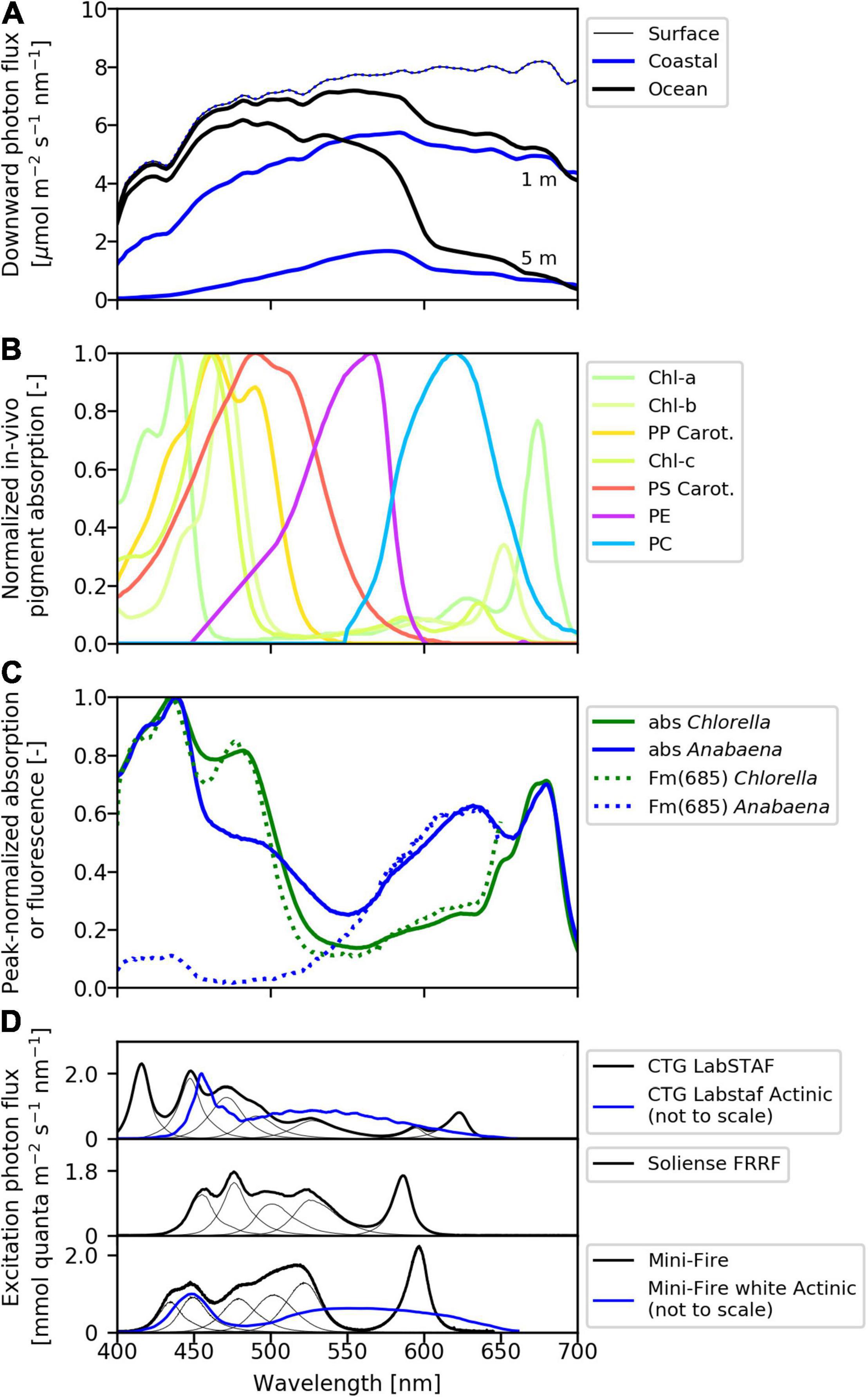
Figure 3. Spectral light availabilities and absorption capabilities. (A) Downward solar photon flux (clear sky, sun at zenith) in a coastal sea and ocean setting. The (attenuated) downwelling photon flux spectrum is given at the surface and at 1 and 5 m depth for both locations. The coastal sea station is modeled after data from the Gulf of Finland, Baltic Sea. The ocean condition is modeled after data from the tropical Pacific Ocean collected during the 2007 SORTIE cruise and obtained from SeaBASS. (B) In-vivo pigment-specific absorption spectra normalized to their maximum value. Chl, chlorophyll (a/b/c); PSC, photosynthetic carotenoids; PPP, photoprotective carotenoids (Bidigare et al., 1990); PE, phycoerythrin; and PC, phycocyanin (including allophycocyanin; Simis and Kauko, 2012). (C) Pigment absorption (solid lines) and F_m(685) fluorescence excitation spectra (dashed lines) of Chlorella sp. (green) and Anabaena cylindrica (blue). (D) Spectra of LEDs typically used to provide excitation light [E_EX(λ), black curves] in three different single-turnover multi-excitation instrument types. For all instruments, the spectrum E_EX(λ) is adjustable (i.e., one or combinations of several LEDs can be used). Spectral quality of actinic light used during light-response curves [E_BG(λ), blue curves, not to scale] provided by white LEDs are given for the LabSTAF and Mini-Fire instruments. In the Mini-Fire instrument, the blue LED (450 nm) can alternatively be used as actinic light source and any of the LEDs available for E_EX can be used as E_BG in the Soliense instrument.

Fundamental to spectral correction procedures is the ability to calculate total PAR absorbed by phytoplankton assemblages ($E_{\text{abs}}^{\text{PAR}}$) as:

$E_{\text{abs}}^{\text{PAR}}=\underset{400}{\overset{700}{\int }}a\left(\mathrm{\lambda }\right)E_{\text{source}}\left(\mathrm{\lambda }\right)d\mathrm{\lambda }(10)$

Where a(λ) is the phytoplankton absorption spectrum and E_source(λ) is the spectrum of the light source. For example, E_source(λ) might correspond to the background light during light response curves (E_BG(λ)), available irradiance in-situ (E_IS(λ)), or a spectrally flat reference spectrum (E_ref(λ); Figure 3). As long as measurements or estimates of these spectra are available, spectral correction procedures can be applied (e.g., Moore et al., 2006).

Not surprisingly, the primary ChlF parameters most affected by the spectral quality of the excitation light source are those related to light capture, including σ_PII and the absolute value of F_o when the latter is being used to quantify light absorption by PSII (Eq. 5; Oxborough et al., 2012). Because the majority of eukaryotic phytoplankton absorb light most strongly in the blue part of the spectrum (Figure 3C), the use of a blue excitation source will usually result in a much larger value of σ_PII than excitation at other wavelengths (e.g., Gorbunov et al., 2020). In marked contrast, cyanobacteria often show a small response to blue excitation because their σ_PII is small in the blue waveband (e.g., Suggett et al., 2004). It is therefore important to report absolute values of σ_PII as a function of excitation light wavelength, σ_PII(λ), and spectrally correct if inter-comparable or ecologically relevant absolute values are desired.

${\mathrm{\sigma }}_{\text{PII},\text{BG}}={\mathrm{\sigma }}_{\text{PII},Ex}\cdot \frac{{\int }_{400}^{700}a\left(\mathrm{\lambda }\right)E_{\text{BG}}\left(\mathrm{\lambda }\right)d\mathrm{\lambda }\cdot {\int }_{400}^{700}{E}_{\text{EX}}\left(\mathrm{\lambda }\right)d\mathrm{\lambda }}{{\int }_{400}^{700}a\left(\mathrm{\lambda }\right)E_{\text{EX}}\left(\mathrm{\lambda }\right)d\mathrm{\lambda }\cdot {\int }_{400}^{700}{E}_{\text{BG}}\left(\mathrm{\lambda }\right)d\mathrm{\lambda }}(11)$

In Eq. 11, σ_PII is corrected to match the spectral quality of background light used during light response curves (E_BG(λ)), which is necessary if spectral quality of excitation light (E_EX(λ)) differs from that of background light (Figure 3D). The same approach can be used to calculate values of σ_PII relevant to E_IS(λ) or E_ref(λ). In order to obtain inter-comparable data, derived J_PII values (section “PSII photochemical flux, J_PII′’) require spectral correction, or should be reported as a wavelength specific value.

Spectral correction is also necessary to derive light response curve parameters (α, E_k) that are relevant to in-situ light availability or if comparing values from simultaneous experiments (e.g., ¹⁴C-uptake) conducted with light of different spectral quality.

$E_{k,\text{IS}}=E_{k,\text{BG}}\cdot \frac{{\int }_{400}^{700}a\left(\mathrm{\lambda }\right)E_{\text{BG}}\left(\mathrm{\lambda }\right)d\mathrm{\lambda }\cdot {\int }_{400}^{700}{E}_{\text{IS}}(\mathrm{\lambda })d\mathrm{\lambda }}{{\int }_{400}^{700}a\left(\mathrm{\lambda }\right)E_{\text{IS}}\left(\mathrm{\lambda }\right)d\mathrm{\lambda }\cdot {\int }_{400}^{700}{E}_{\text{BG}}\left(\mathrm{\lambda }\right)d\mathrm{\lambda }}(12)$

In Eq. 12, the E_k value measured in a ST-ChlF instrument using a given background light spectrum (E_BG(λ)) is corrected to in-situ light availability (E_IS(λ)). Alternatively, all light levels used can be corrected prior to fitting the light response curve.

Inter-comparison among datasets requires that all ST-ChlF measurements are reported alongside spectral information of E_EX(λ) and E_BG(λ). Furthermore, it would be useful for all instruments to have at least one common excitation wavelength. Ideally, E_EX(λ) and E_BG(λ) would be of the same spectral quality, however, this can be difficult to achieve in practice due to engineering constraints. In-situ spectral light distribution should ideally be recorded simultaneously with the ST-ChlF measurement, although this can also be modeled with relatively high accuracy (Mobley, 1994; Lee et al., 2015).

Estimates of spectral light absorption a(λ) required for spectral correction of ST-ChlF data have, until recently, relied on discrete measurements of phytoplankton specific absorption spectra using the filter-pad approach, reconstruction of absorption specific to photosynthetic pigments from pigment concentrations, or PSII fluorescence excitation spectra (e.g., Moore et al., 2006; Silsbe et al., 2015). In recent years, however, the development of multi-excitation wavelength ST-ChlF instruments has provided an approach to characterize spectrally resolved photosynthetic responses of phytoplankton. With these instruments, relative light absorption profiles specific to PSII photochemistry, akin to PSII fluorescence excitation spectra, can now be derived with a high sampling resolution. Such multi-wavelength capabilities of next-generation instruments will greatly simplify spectral correction of ST-ChlF data.

Beyond excitation and background light sources, different ST-ChlF instruments deploy different spectral bands for detection of fluorescence emission, which will differentially bias their responses to chlorophyll fluorescence (from PSII) vs. fluorescence from other sources (including PSI, phycobiliproteins or organic matter). These instrument properties must similarly be reported and archived alongside derived measurements.

Data Reporting and Archiving

The development of best practices for the acquisition of ST-ChlF measurements is a critical step in the collection of coherent and inter-comparable datasets. However, in order to fully leverage the power of global data compilations, it is also necessary that raw data are freely available in a non-proprietary format, and archived with sufficient ancillary information to evaluate data quality and apply any corrections and/or future re-analysis. With this in mind, data collection and archiving should be guided by the “FAIR” principle, making information findable, accessible, interoperable, and reusable (Wilkinson et al., 2016). Implicit in this definition is a commitment to archive all data in consistent and accessible formats facilitating (re-)analysis with open-source computing tools in a manner that is platform agnostic.

Archiving of data (including raw ST-ChlF transients and primary and secondary ST-ChlF parameters) alongside all necessary ancillary information is a key requirement for efficient exchange and communication among research groups using different ST-ChlF instruments. Accessibility of raw ST-ChlF transient data will facilitate coherent re-analysis and quality control of large global datasets, helping to ensure backward and forward compatibility of measurements. Ancillary information (e.g., details of the ST protocols, wavelengths of LEDs and spectral bands of detectors, NPQ-relaxation time and light level, calibrations) is needed to evaluate potential biases in the reported data. Ideally, self-describing data formats allowing for efficient multi-dimensional storage and extraction, such as the netCDF standard, can be broadly adopted alongside a curated data ontology. For more holistic data interpretation, archived ST-ChlF measurements should be linked to additional supporting datasets that include key environmental (nutrients, temperature, surface PAR, mixed layer depth, time of day, sampling depth) and taxonomic (phytoplankton assemblage composition) variables. Guidance on how and where to archive ST-ChlF data will be provided to the user community as part of the Community-Best-Practice document (SCOR Working Group 156, 2021).

Once a robust database framework is established, end-users must be able to access and re-process raw data in a consistent and traceable way, choosing from a range of existing (and evolving) model fits. Toward this end, our group is developing a series of Python-based Jupyter notebooks allowing users with various levels of experience and expertise to re-analyze ST-ChlF data collected with any instrument (Ryan-Keogh and Robinson, 2021). The software will continue to evolve, as new analysis approaches are developed, allowing direct comparison among different approaches to calculate J_PII or fit light-response curves. Drawing inspiration from the CO2SYS program used for thermodynamic calculations of the seawater carbonate system (Lewis and Wallace, 1998), we believe that the ability to re-process raw ST-ChlF data from different sources will maximize consistency and inter-comparability across research groups.

Integration and Application

Deriving Carbon-Based Primary Productivity

Over the past two decades, there has been strong interest in deriving carbon-based primary productivity from ST-ChlF measurements (Hughes et al., 2018). This approach is based on the premise that a significant fraction of J_PII is used for the generation of ATP and NADPH, which in turn is utilized for carbon fixation (Figure 1). In practice, however, the measured stoichiometry between J_PII and carbon fixation (often referred to as the electron requirement for carbon fixation, Φ_e,C, mol e^– [mol C]^–1) varies significantly. Many studies have experimentally determined Φ_e,C from parallel J_PII estimations and ¹⁴C-uptake experiments (see Hughes et al., 2018 and references within). Collectively, such studies are beginning to reveal some coherent trends, such as increases in Φ_e,C above its reference minimum of ∼5 under conditions of environmental stress, including excess light or limiting nutrients. Additionally, Φ_e,C appears to be significantly influenced by taxonomic variability, due to differences in metabolic strategies across different phytoplankton groups (Suggett et al., 2009a,b; Hughes et al., 2021). Moving forward, it is important to better understand the underlying mechanistic factors driving variability in Φ_e,C. Ultimately, this variability represents the adjustable coupling of primary photosynthetic energy production and growth due to (taxon-specific) metabolic plasticity. An understanding of such plasticity will provide crucial insights into the environmental controls on photosynthetic energy use, carbon fixation in aquatic ecosystems, and the response of aquatic photosynthesis to environmental change.

To date, meta-analyses of Φ_e,C data from the literature have clearly demonstrated the challenge of separating methodological biases from true physiological variability in this parameter (e.g., Lawrenz et al., 2013). In many cases, procedural differences in J_PII or carbon fixation measurements across studies (e.g., different wavelengths of light used or varying ¹⁴C-uptake incubation times) can introduce a level of variability comparable to that expected from taxonomic and/or environmental influences. For this reason, consistent approaches of data acquisition, reporting, and archiving are fundamental to characterize physiological and taxonomic variability in Φ_e,C. Recommended standards of best practice in the deployment of ST-ChlF instruments (Table 2) and in the subsequent analysis of resulting data are critical steps toward this goal. At the same time, it will be important for users to adopt consistent approaches for ¹⁴C-uptake measurements, taking into consideration key factors including, for example, the incubation duration and the time of day that the incubation was initiated (e.g., Halsey et al., 2011; Milligan et al., 2015; Schuback et al., 2016).

Exploring Environmental Controls on Primary Productivity

Beyond the potential for high resolution estimates of JV_PII and associated carbon fixation rates (with the caveats discussed above), ST-ChlF approaches also provide a means of directly observing bottom-up controls on phytoplankton physiological ecology. In response to environmental variability on various time-scales (e.g., changing light fields and nutrient concentrations), phytoplankton can rapidly adjust the fraction of light energy absorbed and used to generate chemical energy, and the fraction of the chemical energy invested directly in carbon fixation and growth (Halsey and Jones, 2015). ST-ChlF approaches can provide insight into such physiological processes, enabling real-time observations of changing photosynthetic light utilization in response to interacting effects of multiple environmental and metabolic (e.g., cell cycle) factors.

As an example, ST-ChlF-based studies have been instrumental in examining the effect of iron limitation on phytoplankton physiology and productivity in the global oceans. Chronic iron limitation – affecting phytoplankton in >30% of the global ocean (Moore et al., 2013) – directly influences photosynthetic rates, as iron is a vital component of the photosynthetic electron transport chain (Raven et al., 1999; Yruela, 2013). PSII content can be lowered under iron limitation, and energetically disconnected light-harvesting complexes increase the non-inducible baseline fluorescence (section “Blanks and baseline correction”), resulting in the diagnostic decrease in measured F_v/F_m (Figure 2; Behrenfeld and Milligan, 2013). Furthermore, the absorption cross-section of PSII photochemistry (σ_PII) often increases under iron-limiting conditions, necessitating rapidly inducible NPQ under fluctuating light availability (e.g., Schuback and Tortell, 2019). Increased NPQ levels under iron-limited conditions can be extrapolated to observations of diurnal quenching of ChlF from “standard” in-vivo ChlF fluorometers deployed in continuous flow through and in-situ systems (Roesler and Barnard, 2013; Ryan-Keogh and Thomalla, 2020; Schallenberg et al., 2020).

The deployment of ST-ChlF instruments in continuous shipboard underway mode, or on moorings, floats and gliders provides a means of monitoring phytoplankton photo-physiology at a resolution comparable to that obtainable for other key oceanographic variables (light, temperature, etc.). Integration of ST-ChlF instruments with complementary high-resolution bio-optical measurements (e.g., absorption line height for chla concentrations, particulate carbon and cell size from backscatter, etc.) thus provide the means to observe how interacting physical and chemical conditions drive physiological changes resulting in changes in standing stocks. In this respect, it will be particularly powerful to integrate multi-instrument measurements in the analysis of observed diurnal periodicity in various productivity and biomass tracers, including oxygen (O₂/Ar), particulate carbon (from optical backscatter and attenuation), and ST-ChlF derived photo-physiology in the surface ocean. Furthermore, integration of ST-ChlF data with high-resolution “omics” data from established and emerging approaches can be used to link phytoplankton cellular metabolism with optical indices, including those retrieved from remote sensing. These combined datasets will provide a mechanistic framework for the interpretation and continued refinement of various empirical modeling approaches and algorithms.

Special attention should also be given to parallel field deployments of ST-ChlF instruments with pico-second lifetime fluorometers, recently developed for absolute measurements of the quantum yield of ChlF in natural seawater (Lin et al., 2016; Falkowski et al., 2017). These highly complementary measurements can provide valuable insight into the controls of photosynthetic energy conversion in aquatic environments.

Application of Multi-Wavelengths ST-ChlF Instruments

In addition to the “bulk” phytoplankton photo-physiological properties discussed above, multi-spectral ST-ChlF data can provide information on the taxonomic composition of mixed phytoplankton assemblages (e.g., Gorbunov et al., 2020). The use of spectral fluorescence as a continuous monitoring tool of phytoplankton taxonomic composition is not new. Indeed, more than 40 years ago Yentsch and Yentsch (1979) wrote: “For continuous monitoring of phytoplankton in the open ocean, one anticipates the use of a series of fluorometers or a new fluorometric instrument for detecting emission and inducing excitation at several wavelengths.” Today, high-sensitivity, autonomous ST-ChlF instruments can collect data at >5 excitation and several emission wavebands, and these will provide large datasets to be interpreted in the context of community composition.

The presence of characteristic pigment compliments in different phytoplankton taxa (“spectral groups”) has long been exploited to infer information about phytoplankton taxonomic composition from discrete pigment samples (e.g., Mackey et al., 1996; Kramer et al., 2018) or deconvolution of light absorption and reflectance spectra (Bracher et al., 2017). The variable ChlF at ∼680 nm, as measured by ST-ChlF instruments, stems primarily from chla associated with PSII. However, other pigments present in the PSII light harvesting antenna can pass absorbed energy on to chla such that the light absorbed by accessory photosynthetic pigments can induce ChlF. For this reason, fluorescence excitation spectra can vary significantly between phytoplankton groups (e.g., Johnsen and Sakshaug, 2007; Silsbe et al., 2015; Gorbunov et al., 2020).

Single-turnover variable chlorophyll fluorescence instruments are not yet able to fully resolve entire ChlF emission spectra, as is possible with fluorescence spectrometers (e.g., Seppälä and Balode, 1998; Seppälä and Olli, 2008). However, ChlF excitation at five to eight wavebands is sufficient to resolve characteristic “spectral profiles.” Importantly, such profiles do not merely track ChlF emission, but provide – for each waveband – all primary and secondary ST-ChlF parameters described in section “Theoretical foundations and concepts.” Additionally, with the use of different bandpass filters, ST-ChlF instruments can be easily adapted to detect fluorescence emission at multiple wavebands. For example, fluorescence emission at 650–670 nm arising from phycobiliproteins and phycobilisomes found in cyanobacteria and cryptomonads can be used to monitor the occurrence and distribution of these groups (e.g., Seppälä et al., 2007). Looking forward, many exciting possibilities exist for the interpretation of multi-wavelength ST-ChlF data in the context of phytoplankton community composition. However, some words of caution are also necessary.

The main caveat inherent to all approaches deriving phytoplankton community composition from pigment complements (based on pigment concentrations, spectral light absorption, reflectance, or ChlF) is the fact that specific pigments are rarely unique to individual taxa, and their relative concentrations within a group will change in response to light and nutrient availability. Thus, while the photosynthetic efficiency could perhaps be derived from ST-ChlF data for “functional pigment groups,” the specificity of such analysis to any one particular taxa will likely be limited. Another limitation is the effect of “pigment packaging,” where variations in intracellular pigment concentration affect absorption, reflectance, or ChlF spectra. Variability in spectral shape due to pigment packaging is likely greater among species of the same phytoplankton group under different environmental conditions, than among different spectral groups. In the specific case of ST-ChlF measurements, systematic error can also be introduced into spectrally resolved ST-ChlF parameters if less well-absorbed wavelengths do not provide sufficient energy for full saturation of a ChlF transient during the ST saturation phase (section “Uncertainty and error”).

Notwithstanding these caveats, ST-ChlF instruments have great potential for fine-scale monitoring of phytoplankton taxonomic succession or early detection of harmful algal blooms. In the future, it will be particularly important for the research community to identify the most useful excitation and emission wavelengths for the detection and discrimination of specific phytoplankton groups. In the interest of compiling globally coherent and inter-comparable datasets, an effort should be made to match the wavelengths used in different instrument types.

The development of multi-spectral ST-ChlF instruments coincides with the increasing use of spectrally resolved approaches in satellite remote sensing and biogeochemical modeling, which depend on globally coherent datasets. Further development and application of these instruments should consider, for example, the wavebands measured by satellites, or target key taxa as identified by biogeochemical modeling.

ST-ChlF and the Interpretation of Sun Induced ChlF

In ST-ChlF instruments and in-vivo chla fluorometers, phytoplankton ChlF is controlled through application of an artificial light source. Natural sunlight also induces ChlF in phytoplankton, and the resulting emission at ∼680 nm (known as sun-induced fluorescence, SIF) can be detected by spectroradiometers, including those installed on satellites. The SIF signal detected by satellites has most commonly been measured as a normalized fluorescence line height, quantifying the remote sensing reflectance at the available waveband most affected by ChlF against a baseline from two adjacent, unaffected wavebands (e.g., Letelier and Abbott, 1996; Huot et al., 2005; Gupana et al., 2021).

Not surprisingly, the strongest determinant of the SIF signal is the underlying chla biomass in a given water mass. As discussed above, however, fluorescence per chla (or more correctly per absorbed photon) is not constant. For this reason, a number of studies have explored the use of SIF signatures as a diagnostic tool to assess phytoplankton physiological state (e.g., Letelier et al., 1997; Morrison, 2003; Schallenberg et al., 2008; Behrenfeld et al., 2009; O’Malley et al., 2014; Gilerson and Huot, 2017). Remote sensing of phytoplankton physiology over entire ocean basins would significantly advance the development of global primary productivity models. Yet, large uncertainties in the accurate retrieval of the faint SIF signal and in the physiological interpretation of this signal has so far limited the application of this approach in aquatic ecosystems. By comparison, there has been considerably more research exploring the empirical and mechanistic links between SIF, plant physiology, and primary productivity in the terrestrial realm where foliage with high chlorophyll concentrations generate larger signals (e.g., reviews by Porcar-Castell et al., 2014; Frankenberg and Berry, 2017; Mohammed et al., 2019).

The physiological information inherent to the SIF signal are variations in the quantum yield of fluorescence (Φ_f). The theoretical concepts underlying the physiological interpretation of Φ_f variability are the same as those outlined above for ST-ChlF approaches. Namely, the fraction of absorbed light energy re-emitted as ChlF is controlled by physiological changes in the fraction of energy used for photosynthesis and dissipated as heat (Figure 1). Despite this existing theoretical framework, extracting Φ_f from the SIF signal and interpreting variations in Φ_f in terms of physiology has proven to be far from trivial (Huot et al., 2005; Behrenfeld et al., 2009; Browning et al., 2014; Lin et al., 2016).

Great care must be taken when comparing active (ST-ChlF) and passive (SIF) fluorescence, as the approaches (and derived parameters with similar abbreviations) differ in crucial details. Nevertheless, globally coherent high resolution in-situ data from (autonomous) ST-ChlF instruments hold significant promise to improve the ground-truthing and interpretation of remotely sensed SIF. For example, current modeling approaches to derive Φ_f from SIF must account for changes in [chla], light absorption due to pigment packaging, and NPQ. ST-ChlF instruments are capable of collecting high-resolution in-situ data relevant to all these processes, and global data compilations will allow to detect spatial and temporal patterns needed for model parameterization. Furthermore, modern ST-ChlF instruments deployed in-situ or connected to continuous underway systems, have the ability to collect data that can be used to ground-truth the remotely sensed SIF signal itself.

Coordinated effort should thus be initiated to maximize the usefulness of in-situ ST-ChlF data to validate remotely sensed SIF and improve model representation of Φ_f and other physiologically useful parameters. This work is particularly timely, given anticipated improvements of SIF detection with new generation hyperspectral sensors (e.g., Erickson et al., 2019; Köhler et al., 2020; Tenjo et al., 2021) and the increased use of ST-ChlF instruments on autonomous, in-situ platforms. Guidance and inspiration can be taken from the terrestrial remote sensing community, where paired measurements of active and passive ChlF in laboratory and field have been extensively utilized to examine fluorescence-photosynthesis linkages and explain observed diurnal, seasonal, and stress-induced variations in remotely sensed SIF (e.g., Porcar-Castell et al., 2014; Magney et al., 2017; Wyber et al., 2017; Maguire et al., 2020; Choudhary et al., 2021).

The use of ST-ChlF instruments to reveal global-scale patterns in photo-physiological metrics will contribute to the validation and refinement of ecosystem models and remote sensing algorithms, providing an exciting, and thus far under-utilized, opportunity to connect molecular-scale photosynthetic processes with global-scale biogeochemical cycles.

Conclusion and Outlook

Single-turnover variable chlorophyll fluorescence methods provide a powerful tool for high resolution photo-physiological measurements, with significant potential to examine aquatic productivity and its environmental controls over a range of spatial and temporal scales. Recent advances in instrumentation and data analysis are now beginning to significantly expand the application of ST-ChlF methods to a range of research questions. As the field continues to expand, it is essential to promote global coordination in the development of best practice, using flexible, open-source tools to disseminate information, software, and data products. Through the application of consensus recommendations (Table 2), and a robust system of documenting user-specific protocols, inter-comparison among emerging datasets will be greatly facilitated. This, in turn, will enable the synthesis of synoptic ST-ChlF observations at global scales, providing new insights into the response of marine productivity to a range of perturbations.

The UN Decade of Ocean Science for Sustainable Development (2021–2030) alongside the UN Sustainable Development Goals 6 and 14 (dealing with clean and productive inland and marine waters, respectively) will provide the opportunity to revolutionize the collection, storage, and analysis of ocean data, leading to better understanding of global-scale patterns in key ocean properties and their response to various environmental factors. ST-ChlF-derived observations are important supplements to existing observations that represent phytoplankton standing stocks. Current advances in automation of measurements will enable data compilations at unprecedented resolution in both time and space. Such data will provide information on physical-biological coupling, including the impacts of localized hydrographic fronts, river plumes, and glacial discharge. At larger scales, regional patterns of phytoplankton physiology can be examined in relation to climate forcing, providing empirical correlations and mechanistic understanding for the improvement of ecosystem models, and remote sensing algorithms. Through concerted international cooperation, we are confident that the expansion of ST-ChlF measurements will significantly advance our understanding of global aquatic ecosystems.

Author’s Note

SCOR WG156 does not advocate for the use of any one particular instrument or protocol. The aim of this review is to outline necessary best-practices needed to ensure data inter-comparability across all ST-ChlF instruments, regardless of manufacturer.

Author Contributions

NS and PT wrote the manuscript. All other authors contributed through discussions and comments, and editing of the manuscript.

Funding

OP was supported by GACR project 20-17627S. SS was supported through the European Union’s Horizon 2020 research and innovation program under grant agreement No 776480. EC was supported through NERC grant NE/R011605/1. CM and KO was supported through NERC grant NE/P020844/1.

Conflict of Interest

KO is employed by Chelsea Technology Ltd., and ZK is employed by Solience Inc. However, as the work presented in this review article does not advocate for the use of any particular instrument or protocol, their contribution does not convey any commercial or financial benefit that could be construed as a potential conflict of interest.

The remaining authors declare that the research was conducted in the absence of any commercial or financial relationships that could be construed as a potential conflict of interest.

Dedication

We dedicate this article to the memory of our dear friend and colleague, Jacco Kromkamp, who passed away on Oct. 5, 2020. Jacco was a pioneer in the development and application of variable ChlF measurements to assess phytoplankton productivity in aquatic systems, and he believed passionately in the potential of this method to inform our understanding of ecosystem health. His ideas and insights contributed greatly to the development of our field, and his warmth and friendship helped bring our community together. He positively impacted our lives in numerous ways and will be deeply missed.

References

Behrenfeld, M. J., Bale, A. J., Kolber, Z. S., Aiken, J., and Falkowski, P. G. (1996). Confirmation of iron limitation of phytoplankton photosynthesis in the equatorial Pacific Ocean. Nature 383, 508–511. doi: 10.1038/383508a0

CrossRef Full Text | Google Scholar

Behrenfeld, M. J., and Kolber, Z. S. (1999). Widespread iron limitation of phytoplankton in the south Pacific ocean. Science 283, 840–843. doi: 10.1126/science.283.5403.840

PubMed Abstract | CrossRef Full Text | Google Scholar

Behrenfeld, M. J., and Milligan, A. J. (2013). Photophysiological expressions of iron stress in phytoplankton. Ann. Rev. Mar. Sci. 5, 217–246.

Google Scholar

Behrenfeld, M. J., Westberry, T. K., Boss, E. S., O’Malley, R. T., Siegel, D. A., Wiggert, J. D., et al. (2009). Satellite-detected fluorescence reveals global physiology of ocean phytoplankton. Biogeosciences 6, 779–794.

Google Scholar

Behrenfeld, M. J., Worthington, K., Sherrell, R. M., Chavez, F. P., Strutton, P., McPhaden, M., et al. (2006). Controls on tropical Pacific Ocean productivity revealed through nutrient stress diagnostics. Nature 442, 1025–1028.

Google Scholar

Bidigare, R. R., Ondrusek, M. E., Morrow, J. H., and Kiefer, D. A. (1990). “In-vivo absorption properties of algal pigments,” in Proceedings of the SPIE, Ocean Optics X (International Society for Optics and Photonics), ed. R. W. Spinrad (Orlando, FL: SPIE), 290. doi: 10.1117/12.21451

CrossRef Full Text | Google Scholar

Bilger, W., and Björkman, O. (1991). Temperature dependence of violaxanthin de-epoxidation and non-photochemical fluorescence quenching in intact leaves of Gossypium hirsutum L. and Malva parviflora L. Planta 184, 226–234. doi: 10.1007/BF00197951

PubMed Abstract | CrossRef Full Text | Google Scholar

Boatman, T. G., Geider, R. J., and Oxborough, K. (2019). Improving the accuracy of single turnover active fluorometry (STAF) for the estimation of phytoplankton primary productivity (PhytoPP). Front. Mar. Sci. 6:319. doi: 10.3389/fmars.2019.00319

CrossRef Full Text | Google Scholar

Bouman, H. A., Platt, T., Doblin, M., Figueiras, F. G., Gudmundsson, K., Gudfinnsson, H. G., et al. (2018). Photosynthesis-irradiance parameters of marine phytoplankton: synthesis of a global data set. Earth Syst. Sci. Data 10, 251–266. doi: 10.5194/essd-10-251-2018

CrossRef Full Text | Google Scholar

Bracher, A., Bouman, H. A., Brewin, R. J. W., Bricaud, A., Brotas, V., Ciotti, A. M., et al. (2017). Obtaining phytoplankton diversity from ocean color: a scientific roadmap for future development. Front. Mar. Sci. 4:55. doi: 10.3389/fmars.2017.00055

CrossRef Full Text | Google Scholar

Brett, A., Leape, J., Abbott, M., Sakaguchi, H., Cao, L., Chand, K., et al. (2020). Ocean data need a sea change to help navigate the warming world. Nature 582, 181–183. doi: 10.1038/d41586-020-01668-z

PubMed Abstract | CrossRef Full Text | Google Scholar

Brown, M., Penta, W. B., Jones, B., and Behrenfeld, M. (2019). The ratio of single-turnover to multiple-turnover fluorescence varies predictably with growth rate and cellular chlorophyll in the green alga Dunaliella tertiolecta. Photosynth. Res. 140, 65–76. doi: 10.1007/s11120-018-00612-7

PubMed Abstract | CrossRef Full Text | Google Scholar

Browning, T. J., Bouman, H. A., and Moore, C. M. (2014). Satellite-detected fluorescence: decoupling nonphotochemical quenching from iron stress signals in the South Atlantic and Southern Ocean. Glob. Biogeochem. Cycles 28, 510–524. doi: 10.1002/2013GB004773

CrossRef Full Text | Google Scholar

Butler, W. L. (1978). Energy distribution in the photochemical apparatus of photosynthesis. Annu. Rev. Plant Physiol. 29, 345–378. doi: 10.1146/annurev.pp.29.060178.002021

CrossRef Full Text | Google Scholar

Campbell, D., Hurry, V., Clarke, A. K., Gustafsson, P., and Öquist, G. (1998). Chlorophyll fluorescence analysis of cyanobacterial photosynthesis and acclimation. Microbiol. Mol. Biol. Rev. 62, 667–683. doi: 10.1128/mmbr.62.3.667-683.1998

PubMed Abstract | CrossRef Full Text | Google Scholar

Carvalho, F., Gorbunov, M. Y., Oliver, M. J., Haskins, C., Aragon, D., Kohut, J. T., et al. (2020). FIRe glider: mapping in situ chlorophyll variable fluorescence with autonomous underwater gliders. Limnol. Oceanogr. Methods 18, 531–545. doi: 10.1002/lom3.10380

CrossRef Full Text | Google Scholar

Choudhary, K. K., Chakraborty, A., and Kumari, M. (2021). “Concepts and applications of chlorophyll fluorescence: a remote sensing perspective,” in Geospatial Technologies for Crops and Soils, eds T. Mitran, R. S. Meena, and A. Chakraborty (Singapore: Springer Singapore), 245–276. doi: 10.1007/978-981-15-6864-0_7

CrossRef Full Text | Google Scholar

Cullen, J. J., and Davis, R. F. (2003). The blank can make a big difference in oceanographic measurements. Limnol. Oceanogr. Bull. 12, 29–35. doi: 10.1007/s00360-007-0169-0

PubMed Abstract | CrossRef Full Text | Google Scholar

Dau, H. (1994). Molecular mechanisms and quantitative models of variable photosystem II fluorescence. Photochem. Photobiol. 60, 1–23. doi: 10.1111/j.1751-1097.1994.tb03937.x

CrossRef Full Text | Google Scholar

Erickson, Z. K., Frankenberg, C., Thompson, D. R., Thompson, A. F., and Gierach, M. (2019). Remote sensing of chlorophyll fluorescence in the ocean using imaging spectrometry: toward a vertical profile of fluorescence. Geophys. Res. Lett. 46, 1571–1579. doi: 10.1029/2018GL081273

CrossRef Full Text | Google Scholar

Falkowski, P. G., Barber, R. T., and Smetacek, V. (1998). Biogeochemical controls and feedbacks on ocean primary production. Science 281, 200–206. doi: 10.1126/science.281.5374.200

PubMed Abstract | CrossRef Full Text | Google Scholar

Falkowski, P. G., Lin, H., and Gorbunov, M. Y. (2017). What limits photosynthetic energy conversion efficiency in nature? Lessons from the oceans. Philos. Trans. R. Soc. Lond. B Biol. Sci. 372:20160376. doi: 10.1098/rstb.2016.0376

PubMed Abstract | CrossRef Full Text | Google Scholar

Falkowski, P. G., Ziemann, D., Kolber, Z., and Bienfang, P. K. (1991). Role of eddy pumping in enhancing primary production in the ocean. Nature 352, 55–58. doi: 10.1038/352055a0

CrossRef Full Text | Google Scholar

Farquhar, G. D., Von Caemmerer, S., and Berry, J. A. (2001). Models of photosynthesis. Plant Physiol. 125, 42–45. doi: 10.1104/pp.125.1.42

PubMed Abstract | CrossRef Full Text | Google Scholar

Frankenberg, C., and Berry, J. (2017). “Solar induced chlorophyll fluorescence: origins, relation to photosynthesis and retrieval,” in Comprehensive Remote Sensing (Elsevier), 143–162. doi: 10.1016/B978-0-12-409548-9.10632-3

CrossRef Full Text | Google Scholar

Fujiki, T., Hosaka, T., Kimoto, H., Ishimaru, T., and Saino, T. (2008). In situ observation of phytoplankton productivity by an underwater profiling buoy system: use of fast repetition rate fluorometry. Mar. Ecol. Prog. Ser. 353, 81–88. doi: 10.3354/meps07151

CrossRef Full Text | Google Scholar

Genty, B., Briantais, J. M., and Baker, N. R. (1989). The relationship between the quantum yield of photosynthetic electron transport and quenching of chlorophyll fluorescence. Biochim. Biophys. Acta 990, 87–92. doi: 10.1016/S0304-4165(89)80016-9

CrossRef Full Text | Google Scholar

Gilerson, A. A., and Huot, Y. (2017). “Bio-optical Modeling of Sun-Induced Chlorophyll-a Fluorescence,” in Bio-optical Modeling and Remote Sensing of Inland Waters, eds D. R. Mishra, I. Ogashawara, and A. A. Gitelson (Amsterdam: Elsevier Inc.), 189–231. doi: 10.1016/B978-0-12-804644-9.00007-0

CrossRef Full Text | Google Scholar

Gorbunov, M. Y., and Falkowski, P. G. (2020). Using chlorophyll fluorescence kinetics to determine photosynthesis in aquatic ecosystems. Limnol. Oceanogr. 66, 1–13. doi: 10.1002/LNO.11581

CrossRef Full Text | Google Scholar

Gorbunov, M. Y., Kolber, Z. S., and Falkowski, P. G. (1999). Measuring photosynthetic parameters in individual algal cells by fast repetition rate fluorometry. Photosynth. Res. 62, 141–153. doi: 10.1023/a:1006360005033

CrossRef Full Text | Google Scholar

Gorbunov, M. Y., Kolber, Z. S., Lesser, M. P., and Falkowski, P. G. (2001). Photosynthesis and photoprotection in symbiotic corals. Limnol. Oceanogr. 46, 75–85. doi: 10.4319/lo.2001.46.1.0075

CrossRef Full Text | Google Scholar

Gorbunov, M. Y., Kuzminov, F. I., Fadeev, V. V., Kim, J. D., and Falkowski, P. G. (2011). A kinetic model of non-photochemical quenching in cyanobacteria. Biochim. Biophys. Acta Bioenerg. 1807, 1591–1599. doi: 10.1016/j.bbabio.2011.08.009

PubMed Abstract | CrossRef Full Text | Google Scholar

Gorbunov, M. Y., Shirsin, E., Nikonova, E., Fadeev, V. V., and Falkowski, P. G. (2020). A multi-spectral fluorescence induction and relaxation (fire) technique for physiological and taxonomic analysis of phytoplankton communities. Mar. Ecol. Prog. Ser. 644, 1–13. doi: 10.3354/meps13358

CrossRef Full Text | Google Scholar

Goss, R., and Lepetit, B. (2015). Biodiversity of NPQ. J. Plant Physiol. 172, 13–32. doi: 10.1016/j.jplph.2014.03.004

PubMed Abstract | CrossRef Full Text | Google Scholar

Govindjee (1995). Sixty-three years since Kautsky: chlorophyll a fluorescence. Funct. Plant Biol. 22:131. doi: 10.1071/pp9950131

CrossRef Full Text | Google Scholar

Gupana, R. S., Odermatt, D., Cesana, I., Giardino, C., Nedbal, L., and Damm, A. (2021). Remote sensing of sun-induced chlorophyll-a fluorescence in inland and coastal waters: current state and future prospects. Remote Sens. Environ. 262:112482. doi: 10.1016/j.rse.2021.112482

CrossRef Full Text | Google Scholar

Halsey, K. H., and Jones, B. M. (2015). Phytoplankton strategies for photosynthetic energy allocation. Ann. Rev. Mar. Sci. 7, 265–297. doi: 10.1146/annurev-marine-010814-015813

PubMed Abstract | CrossRef Full Text | Google Scholar

Halsey, K. H., Milligan, A. J., and Behrenfeld, M. J. (2011). Linking time-dependent carbon-fixation efficiencies in Dunaliella Tertiolecta (Chlorophyceae) to underlying metabolic pathways. J. Phycol. 47, 66–76. doi: 10.1111/j.1529-8817.2010.00945.x

PubMed Abstract | CrossRef Full Text | Google Scholar

Harbinson, J., and Rosenqvist, E. (2003). “An Introduction to Chlorophyll Fluorescence,” in Practical Applications of Chlorophyll Fluorescence in Plant Biology, eds J. R. DeEll and P. M. A. Toivonen (Boston, MA: Springer US), 1–29. doi: 10.1007/978-1-4615-0415-3_1

CrossRef Full Text | Google Scholar

Hendrickson, L., Furbank, R. T., and Chow, W. S. (2004). A simple alternative approach to assessing the fate of absorbed light energy using chlorophyll fluorescence. Photosynth. Res. 82:73. doi: 10.1023/B:PRES.0000040446.87305.f4

CrossRef Full Text | Google Scholar

Hoadley, K. D., and Warner, M. E. (2017). Use of open source hardware and software platforms to quantify spectrally dependent differences in photochemical efficiency and functional absorption cross section within the dinoflagellate Symbiodinium spp. Front. Mar. Sci. 4:365. doi: 10.3389/fmars.2017.00365

CrossRef Full Text | Google Scholar

Hughes, D. J., Campbell, D. A., Doblin, M. A., Kromkamp, J. C., Lawrenz, E., Moore, C. M., et al. (2018). Roadmaps and detours: active chlorophyll- a assessments of primary productivity across marine and freshwater systems. Environ. Sci. Technol. 52, 12039–12054. doi: 10.1021/acs.est.8b03488

PubMed Abstract | CrossRef Full Text | Google Scholar

Hughes, D. J., Crosswell, J. R., Doblin, M. A., Oxborough, K., Ralph, P. J., Varkey, D., et al. (2020). Dynamic variability of the phytoplankton electron requirement for carbon fixation in eastern Australian waters. J. Mar. Syst. 202:103252. doi: 10.1016/j.jmarsys.2019.103252

CrossRef Full Text | Google Scholar

Hughes, D. J., Giannini, F. C., Ciotti, A. M., Doblin, M. A., Ralph, P. J., Varkey, D., et al. (2021). Taxonomic variability in the electron requirement for carbon fixation across marine phytoplankton. J. Phycol. 57, 111–127. doi: 10.1111/jpy.13068

PubMed Abstract | CrossRef Full Text | Google Scholar

Huot, Y., and Babin, M. (2010). “Overview of Fluorescence Protocols: Theory, Basic Concepts, and Practice,” in Chlorophyll a Fluorescence in Aquatic Sciences: Methods and Applications, eds D. Suggett, O. Prášil, and M. Borowitzka (Dordrecht: Springer Netherlands), 31–74. doi: 10.1007/978-90-481-9268-7_3

CrossRef Full Text | Google Scholar

Huot, Y., Brown, C. A., and Cullen, J. J. (2005). New algorithms for MODIS sun-induced chlorophyll fluorescence and a comparison with present data products. Limnol. Oceanogr. Methods 3, 108–130. doi: 10.4319/lom.2005.3.108

CrossRef Full Text | Google Scholar

Jakob, T., Goss, R., and Wilhelm, C. (1999). Activation of diadinoxanthin de-epoxidase due to a chlororespiratory proton gradient in the dark in the diatom Phaeodactylum tricornutum. Plant Biol. 1, 76–82. doi: 10.1111/j.1438-8677.1999.tb00711.x

CrossRef Full Text | Google Scholar

Johnsen, G., and Sakshaug, E. (2007). Biooptical characteristics of PSII and PSI in 33 species (13 pigment groups) of marine phytoplankton, and the relevance for pulse amplitude-modulated and fast-repetition-rate fluorometry. J. Phycol. 43, 1236–1251. doi: 10.1111/j.1529-8817.2007.00422.x

CrossRef Full Text | Google Scholar

Johnsen, S. (2012). The Optics of Life: A biologist’s Guide to Light in Nature. Princton, NJ: Princton University Press, doi: 10.5860/choice.49-5660

PubMed Abstract | CrossRef Full Text | Google Scholar

Kautsky, H., and Hirsch, A. (1931). Neue versuche zur kohlensäureassimilation. Naturwissenschaften 19:964. doi: 10.1007/BF01516164

CrossRef Full Text | Google Scholar

Kirk, J. T. O. (2010). Light and Photosynthesis in Aquatic Ecosystems, 3rd Edn. Cambridge: Cambridge University Press, doi: 10.1017/CBO9781139168212

CrossRef Full Text | Google Scholar

Klughammer, C., and Schreiber, U. (2008). Complementary PS II quantum yields calculated from simple fluorescence parameters measured by PAM fluorometry and the Saturation Pulse method. PAM Appl. Notes 1, 27–35.

Google Scholar

Köhler, P., Behrenfeld, M. J., Landgraf, J., Joiner, J., Magney, T. S., and Frankenberg, C. (2020). Global retrievals of solar-induced chlorophyll fluorescence at red wavelengths with TROPOMI. Geophys. Res. Lett. 47:e2020GL087541. doi: 10.1029/2020GL087541

CrossRef Full Text | Google Scholar

Kolber, Z. (2021). Light Induced Fluorescence Transient Fluorometer–Operating Manual. Available online at: https://soliense.com/LIFT_Marine.php (accessed June 28, 2021).

Google Scholar

Kolber, Z., and Falkowski, P. G. (1993). Use of active fluorescence to estimate phytoplankton photosynthesis in situ. Limnol. Oceanogr. 38, 1646–1665. doi: 10.4319/lo.1993.38.8.1646

CrossRef Full Text | Google Scholar

Kolber, Z., Wyman, K. V., and Falkowski, P. G. (1990). Natural variability in photosynthetic energy conversion efficiency: a field study in the Gulf of Maine. Limnol. Oceanogr. 35, 72–79. doi: 10.4319/lo.1990.35.1.0072

CrossRef Full Text | Google Scholar

Kolber, Z. S., Barber, R. T., Coale, K. H., Fitzwateri, S. E., Greene, R. M., Johnson, K. S., et al. (1994). Iron limitation of phytoplankton photosynthesis in the equatorial Pacific Ocean. Nature 371, 145–149. doi: 10.1038/371145a0

CrossRef Full Text | Google Scholar

Kolber, Z. S., Prášil, O., and Falkowski, P. G. (1998). Measurements of variable chlorophyll fluorescence using fast repetition rate techniques: defining methodology and experimental protocols. Biochim. Biophys. Acta Bioenerg. 1367, 88–106. doi: 10.1016/S0005-2728(98)00135-2

CrossRef Full Text | Google Scholar

Kramer, D. M., Johnson, G., Kiirats, O., and Edwards, G. E. (2004). New fluorescence parameters for the determination of QA redox state and excitation energy fluxes. Photosynth. Res. 79, 209–218. doi: 10.1023/B:PRES.0000015391.99477.0d

CrossRef Full Text | Google Scholar

Kramer, S. J., Roesler, C. S., and Sosik, H. M. (2018). Bio-optical discrimination of diatoms from other phytoplankton in the surface ocean: evaluation and refinement of a model for the Northwest Atlantic. Remote Sens. Environ. 217, 126–143. doi: 10.1016/j.rse.2018.08.010

CrossRef Full Text | Google Scholar

Krause, G. H., and Weis, E. (1991). Chlorophyll fluorescence and photosynthesis: the basics. Annu. Rev. Plant Physiol. Plant Mol. Biol. 42, 313–349. doi: 10.1146/annurev.pp.42.060191.001525

CrossRef Full Text | Google Scholar

Kromkamp, J. C., and Forster, R. M. (2003). The use of variable fluorescence measurements in aquatic ecosystems: differences between multiple and single turnover measuring protocols and suggested terminology. Eur. J. Phycol. 38, 103–112. doi: 10.1080/0967026031000094094

CrossRef Full Text | Google Scholar

Kruskopf, M., and Flynn, K. J. (2006). Chlorophyll content and fluorescence responses cannot be used to gauge reliably phytoplankton biomass, nutrient status or growth rate. New Phytol. 169, 525–536. doi: 10.1111/j.1469-8137.2005.01601.x

PubMed Abstract | CrossRef Full Text | Google Scholar

Lacour, T., Babin, M., and Lavaud, J. (2020). Diversity in xanthophyll cycle pigments content and related nonphotochemical quenching (NPQ) among microalgae: implications for growth strategy and ecology. J. Phycol. 56, 245–263. doi: 10.1111/jpy.12944

PubMed Abstract | CrossRef Full Text | Google Scholar

Lacour, T., Larivière, J., Ferland, J., Bruyant, F., Lavaud, J., and Babin, M. (2018). The role of sustained photoprotective non-photochemical quenching in low temperature and high light acclimation in the bloom-forming arctic diatom Thalassiosira gravida. Front. Mar. Sci. 5:354. doi: 10.3389/fmars.2018.00354

CrossRef Full Text | Google Scholar

Laney, S. R. (2003). Assessing the error in photosynthetic properties determined by fast repetition rate fluorometry. Limnol. Oceanogr. 48, 2234–2242. doi: 10.4319/lo.2003.48.6.2234

CrossRef Full Text | Google Scholar

Laney, S. R. (2010). “In situ measurement of variable fluorescence transients,” in Chlorophyll a Fluorescence in Aquatic Sciences: Methods and Applications, eds D. Suggett, O. Prášil, and M. Borowitzka (Dordrecht: Springer Netherlands), 19–30. doi: 10.1007/978-90-481-9268-7_2

CrossRef Full Text | Google Scholar

Laney, S. R., and Letelier, R. M. (2008). Artifacts in measurements of chlorophyll fluorescence transients, with specific application to fast repetition rate fluorometry. Limnol. Oceanogr. Methods 6, 40–50. doi: 10.4319/lom.2008.6.40

CrossRef Full Text | Google Scholar

Lavaud, J., and Goss, R. (2014). “The peculiar features of non-photochemical fluorescence quenching in diatoms and brown algae,” in Advances in Photosynthesis and Respiration, eds B. Demmig-Adams, G. Garab, W. Adams III, and Govindjee (Dordrecht: Springer), 421–443. doi: 10.1007/978-94-017-9032-1_20

CrossRef Full Text | Google Scholar

Lavergne, J., and Trissl, H. W. (1995). Theory of fluorescence induction in photosystem II: derivation of analytical expressions in a model including exciton-radical-pair equilibrium and restricted energy transfer between photosynthetic units. Biophys. J. 68, 2474–2492. doi: 10.1016/S0006-3495(95)80429-7

CrossRef Full Text | Google Scholar

Lavorel, J., and Joliot, P. (1972). A connected model of the photosynthetic unit. Biophys. J. 12, 815–831. doi: 10.1016/S0006-3495(72)86125-3

CrossRef Full Text | Google Scholar

Lawrenz, E., Silsbe, G., Capuzzo, E., Ylöstalo, P., Forster, R. M., Simis, S. G. H., et al. (2013). Predicting the electron requirement for carbon fixation in seas and oceans. PLoS One 8:e58137. doi: 10.1371/journal.pone.0058137

PubMed Abstract | CrossRef Full Text | Google Scholar

Lee, Z., Marra, J., Perry, M. J., and Kahru, M. (2015). Estimating oceanic primary productivity from ocean color remote sensing: a strategic assessment. J. Mar. Syst. 149, 50–59. doi: 10.1016/j.jmarsys.2014.11.015

CrossRef Full Text | Google Scholar

Letelier, R. M., and Abbott, M. R. (1996). An analysis of chlorophyll fluorescence algorithms for the moderate resolution imaging spectrometer (MODIS). Remote Sens. Environ. 58, 215–223. doi: 10.1016/S0034-4257(96)00073-9

CrossRef Full Text | Google Scholar

Letelier, R. M., Abbott, M. R., and Karl, D. M. (1997). Chlorophyll natural fluorescence response to upwelling events in the Southern Ocean. Geophys. Res. Lett. 24, 409–412. doi: 10.1029/97GL00205

CrossRef Full Text | Google Scholar

Lewis, E. R., and Wallace, D. W. R. (1998). Program Developed for CO2 System Calculations. United States: N.p., Web. doi: 10.15485/1464255

CrossRef Full Text | Google Scholar

Li, G., Woroch, A. D., Donaher, N. A., Cockshutt, A. M., and Campbell, D. A. (2016). A hard day’s night: diatoms continue recycling photosystem II in the dark. Front. Mar. Sci. 3:218. doi: 10.3389/fmars.2016.00218

CrossRef Full Text | Google Scholar

Lichtenthaler, H. K. (1988). “In vivo chlorophyll fluorescence as a tool for stress detection in plants,” in Applications of Chlorophyll Fluorescence in Photosynthesis Research, Stress Physiology, Hydrobiology and Remote Sensing, ed. H. K. Lichtenthaler (Dordrecht: Springer Netherlands), 129–142. doi: 10.1007/978-94-009-2823-7_16

CrossRef Full Text | Google Scholar

Lin, H., Kuzminov, F. I., Park, J., Lee, S. H., Falkowski, P. G., and Gorbunov, M. Y. (2016). Phytoplankton: the fate of photons absorbed by phytoplankton in the global ocean. Science 351, 264–267. doi: 10.1126/science.aab2213

PubMed Abstract | CrossRef Full Text | Google Scholar

Lombard, F., Boss, E., Waite, A. M., Uitz, J., Stemmann, L., Sosik, H. M., et al. (2019). Globally consistent quantitative observations of planktonic ecosystems. Front. Mar. Sci. 6:196. doi: 10.3389/fmars.2019.00196

CrossRef Full Text | Google Scholar

Macey, A. I., Ryan-Keogh, T., Richier, S., Moore, C. M., and Bibby, T. S. (2014). Photosynthetic protein stoichiometry and photophysiology in the high latitude north atlantic. Limnol. Oceanogr. 59, 1853–1864. doi: 10.4319/lo.2014.59.6.1853

CrossRef Full Text | Google Scholar

Mackey, M. D., Mackey, D. J., Higgins, H. W., and Wright, S. W. (1996). CHEMTAX–a program for estimating class abundances from chemical markers: application to HPLC measurements of phytoplankton. Mar. Ecol. Prog. Ser. 144, 265–283. doi: 10.3354/meps144265

CrossRef Full Text | Google Scholar

Magdaong, N. C. M., and Blankenship, R. E. (2018). Photoprotective, excited-state quenching mechanisms in diverse photosynthetic organisms. J. Biol. Chem. 293, 5018–5025. doi: 10.1074/jbc.TM117.000233

PubMed Abstract | CrossRef Full Text | Google Scholar

Magney, T. S., Frankenberg, C., Fisher, J. B., Sun, Y., North, G. B., Davis, T. S., et al. (2017). Connecting active to passive fluorescence with photosynthesis: a method for evaluating remote sensing measurements of Chl fluorescence. New Phytol. 215, 1594–1608. doi: 10.1111/nph.14662

PubMed Abstract | CrossRef Full Text | Google Scholar

Maguire, A. J., Eitel, J. U. H., Griffin, K. L., Magney, T. S., Long, R. A., Vierling, L. A., et al. (2020). On the functional relationship between fluorescence and photochemical yields in complex evergreen needleleaf canopies. Geophys. Res. Lett. 47:e2020GL087858. doi: 10.1029/2020GL087858

CrossRef Full Text | Google Scholar

McKew, B. A., Davey, P., Finch, S. J., Hopkins, J., Lefebvre, S. C., Metodiev, M. V., et al. (2013). The trade-off between the light-harvesting and photoprotective functions of fucoxanthin-chlorophyll proteins dominates light acclimation in Emiliania huxleyi (clone CCMP 1516). New Phytol. 200, 74–85. doi: 10.1111/nph.12373

PubMed Abstract | CrossRef Full Text | Google Scholar

Méléder, V., Jesus, B., Barnett, A., Barille, L., and Lavaud, J. (2018). Microphytobenthos primary production estimated by hyperspectral reflectance. PLoS One 13:e0197093. doi: 10.1371/journal.pone.0197093

PubMed Abstract | CrossRef Full Text | Google Scholar

Milligan, A. J., Halsey, K. H., and Behrenfeld, M. J. (2015). HORIZONS:advancing interpretations of 14C-uptake measurements in the context of phytoplankton physiology and ecology. J. Plankton Res. 37, 692–698. doi: 10.1093/plankt/fbv051

PubMed Abstract | CrossRef Full Text | Google Scholar

Mobley, C. D. (1994). Light and Water: Radiative Transfer in Natural Waters. San Diego, CA: Academic Press.

Google Scholar

Mohammed, G. H., Colombo, R., Middleton, E. M., Rascher, U., van der Tol, C., Nedbal, L., et al. (2019). Remote sensing of solar-induced chlorophyll fluorescence (SIF) in vegetation: 50 years of progress. Remote Sens. Environ. 231. doi: 10.1016/j.rse.2019.04.030

PubMed Abstract | CrossRef Full Text | Google Scholar

Moore, C. M., Mills, M. M., Arrigo, K. R., Berman-Frank, I., Bopp, L., Boyd, P. W., et al. (2013). Processes and patterns of oceanic nutrient limitation. Nat. Geosci. 6, 701–710. doi: 10.1038/ngeo1765

CrossRef Full Text | Google Scholar

Moore, C. M., Mills, M. M., Langlois, R., Milne, A., Achterberg, E. P., La Roche, J., et al. (2008). Relative influence of nitrogen and phosphorus availability on phytoplankton physiology and productivity in the oligotrophic sub-tropical North Atlantic Ocean. Limnol. Oceanogr. 53, 291–305. doi: 10.4319/lo.2008.53.1.0291

CrossRef Full Text | Google Scholar

Moore, C. M., Suggett, D., Holligan, P. M., Sharples, J., Abraham, E. R., Lucas, M. I., et al. (2003). Physical controls on phytoplankton physiology and production at a shelf sea front: a fast repetition-rate fluorometer based field study. Mar. Ecol. Prog. Ser. 259, 29–45. doi: 10.3354/meps259029

CrossRef Full Text | Google Scholar

Moore, C. M., Suggett, D. J., Hickman, A. E., Kim, Y. N., Tweddle, J. F., Sharples, J., et al. (2006). Phytoplankton photoacclimation and photoadaptation in response to environmental gradients in a shelf sea. Limnol. Oceanogr. 51, 936–949. doi: 10.4319/lo.2006.51.2.0936

CrossRef Full Text | Google Scholar

Morrison, J. R. (2003). In situ determination of the quantum yield of phytoplankton chlorophyll a fluorescence: a simple algorithm, observations, and a model. Limnol. Oceanogr. 48, 618–631. doi: 10.4319/lo.2003.48.2.0618

CrossRef Full Text | Google Scholar

Ni, G., Zimbalatti, G., Murphy, C. D., Barnett, A. B., Arsenault, C. M., Li, G., et al. (2017). Arctic Micromonas uses protein pools and non-photochemical quenching to cope with temperature restrictions on photosystem II protein turnover. Photosynth. Res. 131, 203–220. doi: 10.1007/s11120-016-0310-6

PubMed Abstract | CrossRef Full Text | Google Scholar

O’Malley, R. T., Behrenfeld, M. J., Westberry, T. K., Milligan, A. J., Shang, S., and Yan, J. (2014). Geostationary satellite observations of dynamic phytoplankton photophysiology. Geophys. Res. Lett. 41, 5052–5059. doi: 10.1002/2014GL060246

CrossRef Full Text | Google Scholar

Oxborough, K. (2021). LabSTAF and RunSTAF Handbook. (Doc No. 2408-014-HB | Issue B). West Molesey: Chelsea Technologies Ltd, 98. doi: 10.25607/OBP-1029

CrossRef Full Text | Google Scholar

Oxborough, K., and Baker, N. R. (1997). Resolving chlorophyll a fluorescence images of photosynthetic efficiency into photochemical and non-photochemical components–calculation of qP and Fv’/Fm’ without measuring Fo’. Photosynth. Res. 54, 135–142. doi: 10.1023/A:1005936823310

CrossRef Full Text | Google Scholar

Oxborough, K., Moore, C. M., Suggett, D. J., Lawson, T., Chan, H. G., and Geider, R. J. (2012). Direct estimation of functional PSII reaction center concentration and PSII electron flux on a volume basis: a new approach to the analysis of fast repetition rate fluorometry (FRRf) data. Limnol. Oceanogr. Methods 10, 142–154. doi: 10.4319/lom.2012.10.142

CrossRef Full Text | Google Scholar

Papageorgiu, G. C., and Govindjee (2004). Chlorophyll a fluorescence. Adv. Photosynth. Respir. 19:820. doi: 10.1007/978-1-4020-3218-9

CrossRef Full Text | Google Scholar

Parkhill, J. P., Maillet, G., and Cullen, J. J. (2001). Fluorescence-based maximal quantum yield for PSII as a diagnostic of nutrient stress. J. Phycol. 37, 517–529. doi: 10.1046/j.1529-8817.2001.037004517.x

CrossRef Full Text | Google Scholar

Platt, T., and Gallegos, C. L. (1980). “Modelling primary production,” in Primary Productivity in the Sea, ed. P. G. Falkowski (Boston, MA: Springer US), 339–362. doi: 10.1007/978-1-4684-3890-1_19

CrossRef Full Text | Google Scholar

Porcar-Castell, A., Tyystjärvi, E., Atherton, J., Van Der Tol, C., Flexas, J., Pfündel, E. E., et al. (2014). Linking chlorophyll a fluorescence to photosynthesis for remote sensing applications: mechanisms and challenges. J. Exp. Bot. 65, 4065–4095. doi: 10.1093/jxb/eru191

PubMed Abstract | CrossRef Full Text | Google Scholar

Raven, J. A., Evans, M. C. W., and Korb, R. E. (1999). The role of trace metals in photosynthetic electron transport in O2-evolving organisms. Photosynth. Res. 60, 111–150. doi: 10.1023/A:1006282714942

CrossRef Full Text | Google Scholar

Roesler, C. S., and Barnard, A. H. (2013). Optical proxy for phytoplankton biomass in the absence of photophysiology: rethinking the absorption line height. Methods Oceanogr. 7, 79–94. doi: 10.1016/j.mio.2013.12.003

CrossRef Full Text | Google Scholar

Roháček, K., and Barták, M. (1999). Technique of the modulated chlorophyll fluorescence: basic concepts, useful parameters, and some applications. Photosynthetica 37, 339–363. doi: 10.1023/A:1007172424619

CrossRef Full Text | Google Scholar

Roháček, K., Bertrand, M., Moreau, B., Jacquette, B., Caplat, C., Morant-Manceau, A., et al. (2014). Relaxation of the non-photochemical chlorophyll fluorescence quenching in diatoms: kinetics, components and mechanisms. Philos. Trans. R. Soc. B Biol. Sci. 369:20130241. doi: 10.1098/rstb.2013.0241

PubMed Abstract | CrossRef Full Text | Google Scholar

Roháček, K., Soukupová, J., and Barták, M. (2008). “Chlorophyll fluorescence: a wonderful tool to study plant physiology and plant stress,” in Plant Cell Compartments–Selected Topics, 1st Edn, ed. B. Schoefs (Kerala: Research Signpost), 41–104.

Google Scholar

Ryan-Keogh, T. J., and Thomalla, S. J. (2020). Deriving a proxy for iron limitation from chlorophyll fluorescence on buoyancy gliders. Front. Mar. Sci. 7:275. doi: 10.3389/fmars.2020.00275

CrossRef Full Text | Google Scholar

Ryan-Keogh, T. J., Thomalla, S. J., Little, H., and Melanson, J.-R. (2018). Seasonal regulation of the coupling between photosynthetic electron transport and carbon fixation in the Southern Ocean. Limnol. Oceanogr. 63, 1856–1876. doi: 10.1002/lno.10812

CrossRef Full Text | Google Scholar

Ryan-Keogh, T. J., and Robinson, C. M. (2021). Phytoplankton photophysiology utilities: a python toolbox for the standardisation of processing active chlorophyll fluorescence data. Front. Mar. Sci. 8:526. doi: 10.3389/fmars.2021.525414

CrossRef Full Text | Google Scholar

Schallenberg, C., Lewis, M. R., Kelley, D. E., and Cullen, J. J. (2008). Inferred influence of nutrient availability on the relationship between sun-induced chlorophyll fluorescence and incident irradiance in the Bering Sea. J. Geophys. Res. Ocean 113, 1–21. doi: 10.1029/2007JC004355

CrossRef Full Text | Google Scholar

Schallenberg, C., Strzepek, R. F., Schuback, N., Clementson, L. A., Boyd, P. W., and Trull, T. W. (2020). Diel quenching of Southern Ocean phytoplankton fluorescence is related to iron limitation. Biogeosciences 17, 793–812. doi: 10.5194/bg-17-793-2020

CrossRef Full Text | Google Scholar

Schreiber, U., Klughammer, C., and Schansker, G. (2019). Rapidly reversible chlorophyll fluorescence quenching induced by pulses of supersaturating light in vivo. Photosynth. Res. 142, 35–50. doi: 10.1007/s11120-019-00644-7

PubMed Abstract | CrossRef Full Text | Google Scholar

Schuback, N., Flecken, M., Maldonado, M. T., and Tortell, P. D. (2016). Diurnal variation in the coupling of photosynthetic electron transport and carbon fixation in iron-limited phytoplankton in the NE subarctic Pacific. Biogeosciences 13, 1019–1035. doi: 10.5194/bg-13-1019-2016

CrossRef Full Text | Google Scholar

Schuback, N., Schallenberg, C., Duckham, C., Maldonado, M. T., and Tortell, P. D. (2015). Interacting effects of light and iron availability on the coupling of photosynthetic electron transport and CO2-assimilation in marine phytoplankton. PLoS One 10:e0133235. doi: 10.1371/journal.pone.0133235

PubMed Abstract | CrossRef Full Text | Google Scholar

Schuback, N., Schallenberg, C., and Tortell, P. D. (2020). “Non-photochemical quenching of chl-a fluorescence: an undervalued optical indicator of photosynthetic efficiency,” in Proceedings of the Ocean Science Meeting 2020, San Diego, CA, doi: 10.13140/RG.2.2.31978.26569

CrossRef Full Text | Google Scholar

Schuback, N., and Tortell, P. D. (2019). Diurnal regulation of photosynthetic light absorption, electron transport and carbon fixation in two contrasting oceanic environments. Biogeosciences 16, 1381–1399. doi: 10.5194/bg-16-1381-2019

CrossRef Full Text | Google Scholar

SCOR Working Group 156 (2021). A User Guide for the Application of Single Turnover Active Chlorophyll Fluorescence for Phytoplankton Productivity Measurements. Version 1. Baltimore, MD: Scientific Committee on Oceanic Research Working Group 156, 20. doi: 10.25607/OBP-1084

CrossRef Full Text | Google Scholar

Seppälä, J., and Balode, M. (1998). “The use of spectral fluorescence methods to detect changes in the phytoplankton community,” in Eutrophication in Planktonic Ecosystems: Food Web Dynamics and Elemental Cycling, eds T. Tamminen and H. Kuosa (Dordrecht: Springer Netherlands), 207–217. doi: 10.1007/978-94-017-1493-8_16

CrossRef Full Text | Google Scholar

Seppälä, J., and Olli, K. (2008). Multivariate analysis of phytoplankton spectral in vivo fluorescence: estimation of phytoplankton biomass during a mesocosm study in the Baltic Sea. Mar. Ecol. Prog. Ser. 370, 69–85. doi: 10.3354/meps07647

CrossRef Full Text | Google Scholar

Seppälä, J., Ylöstalo, P., Kaitala, S., Hällfors, S., Raateoja, M., and Maunula, P. (2007). Ship-of-opportunity based phycocyanin fluorescence monitoring of the filamentous cyanobacteria bloom dynamics in the Baltic Sea. Estuar. Coast. Shelf Sci. 73, 489–500. doi: 10.1016/j.ecss.2007.02.015

CrossRef Full Text | Google Scholar

Silsbe, G. M., and Kromkamp, J. C. (2012). Modeling the irradiance dependency of the quantum efficiency of photosynthesis. Limnol. Oceanogr. Methods 10, 645–652. doi: 10.4319/lom.2012.10.645

CrossRef Full Text | Google Scholar

Silsbe, G. M., Oxborough, K., Suggett, D. J., Forster, R. M., Ihnken, S., Komárek, O., et al. (2015). Toward autonomous measurements of photosynthetic electron transport rates: an evaluation of active fluorescence-based measurements of photochemistry. Limnol. Oceanogr. Methods 13, 138–155. doi: 10.1002/lom3.10014

CrossRef Full Text | Google Scholar

Simis, S. G. H., and Kauko, H. M. (2012). In vivo mass-specific absorption spectra of phycobilipigments through selective bleaching. Limnol. Oceanogr. Methods 10, 214–226. doi: 10.4319/lom.2012.10.214

CrossRef Full Text | Google Scholar

Stirbet, A. (2013). Excitonic connectivity between photosystem II units: what is it, and how to measure it? Photosynth. Res. 116, 189–214. doi: 10.1007/s11120-013-9863-9

PubMed Abstract | CrossRef Full Text | Google Scholar

Suggett, D. J., MacIntyre, H. L., and Geider, R. J. (2004). Evaluation of biophysical and optical determinations of light absorption by photosystem II in phytoplankton. Limnol. Oceanogr. Methods 2, 316–332. doi: 10.4319/lom.2004.2.316

CrossRef Full Text | Google Scholar

Suggett, D. J., MacIntyre, H. L., Kana, T. M., and Geider, R. J. (2009a). Comparing electron transport with gas exchange: parameterising exchange rates between alternative photosynthetic currencies for eukaryotic phytoplankton. Aquat. Microb. Ecol. 56, 147–162. doi: 10.3354/ame01303

CrossRef Full Text | Google Scholar

Suggett, D. J., Moore, C. M., and Geider, R. J. (2010a). Chlorophyll a Fluorescence in Aquatic Sciences: Methods and Applications. Dordrecht: Springer, doi: 10.1007/978-90-481-9268-7

CrossRef Full Text | Google Scholar

Suggett, D. J., Moore, C. M., and Geider, R. J. (2010b). “Estimating aquatic productivity from active fluorescence measurements,” in Chlorophyll a Fluorescence in Aquatic Sciences: Methods and Applications, eds D. Suggett, O. Prášil, and M. Borowitzka (Dordrecht: Springer), 103–127. doi: 10.1007/978-90-481-9268-7_6

CrossRef Full Text | Google Scholar

Suggett, D. J., Moore, C. M., Hickman, A. E., and Geider, R. J. (2009b). Interpretation of fast repetition rate (FRR) fluorescence: signatures of phytoplankton community structure versus physiological state. Mar. Ecol. Prog. Ser. 376, 1–19. doi: 10.3354/meps07830

CrossRef Full Text | Google Scholar

Tanhua, T., Pouliquen, S., Hausman, J., O’Brien, K. M., Bricher, P., de Bruin, T., et al. (2019). Ocean FAIR data services. Front. Mar. Sci. 6:440. doi: 10.3389/fmars.2019.00440

CrossRef Full Text | Google Scholar

Tenjo, C., Ruiz-verdú, A., Van Wittenberghe, S., Delegido, J., and Moreno, J. (2021). A new algorithm for the retrieval of sun induced chlorophyll fluorescence of water bodies exploiting the detailed spectral shape of water-leaving radiance. Remote Sens. 13, 1–19. doi: 10.3390/rs13020329

CrossRef Full Text | Google Scholar

Thomalla, S. J., Moutier, W., Ryan-Keogh, T. J., Gregor, L., and Schütt, J. (2018). An optimized method for correcting fluorescence quenching using optical backscattering on autonomous platforms. Limnol. Oceanogr. Methods 16, 132–144. doi: 10.1002/lom3.10234

CrossRef Full Text | Google Scholar

Trissl, H., and Lavergne, J. (1995). Fluorescence induction from photosystem II: analytical equations for the yields of photochemistry and fluorescence derived from analysis of a model including exciton-radical pair equilibrium and restricted energy transfer between photosynthetic units. Funct. Plant Biol. 22:183. doi: 10.1071/pp9950183

CrossRef Full Text | Google Scholar

Wilkinson, M. D., Dumontier, M., Aalbersberg, I. J., Appleton, G., Axton, M., Baak, A., et al. (2016). Comment: the FAIR guiding principles for scientific data management and stewardship. Sci. Data 3, 1–9. doi: 10.1038/sdata.2016.18

PubMed Abstract | CrossRef Full Text | Google Scholar

Wyber, R., Malenovský, Z., Ashcroft, M. B., Osmond, B., and Robinson, S. A. (2017). Do daily and seasonal trends in leaf solar induced fluorescence reflect changes in photosynthesis, growth or light exposure? Remote Sens. 9:604. doi: 10.3390/rs9060604

CrossRef Full Text | Google Scholar

Xu, K., Lavaud, J., Perkins, R., Austen, E., Bonnanfant, M., and Campbell, D. A. (2018). Phytoplankton σPSII and excitation dissipation; implications for estimates of primary productivity. Front. Mar. Sci. 5:281. doi: 10.3389/FMARS.2018.00281

CrossRef Full Text | Google Scholar

Yentsch, C. S., and Yentsch, C. M. (1979). Fluorescence spectral signatures: the characterization of phytoplankton populations be the use of excitation and emission spectra. J. Mar. Res. 37, 471–483.

Google Scholar

Yruela, I. (2013). Transition metals in plant photosynthesis. Metallomics 5, 1090–1109. doi: 10.1039/c3mt00086a

PubMed Abstract | CrossRef Full Text | Google Scholar