Assessing the Impact of the Assimilation of SWOT Observations in a Global High-Resolution Analysis and Forecasting System Part 1: Methods

Introduction

Nadir altimeter Sea Level Anomaly (SLA) measurements have made major contributions to our understanding of ocean circulation. While along-track SLA data can observe wavelengths as small as 50–70 km (Dufau et al., 2016), the global mesoscale resolution is strongly limited by the space (distance between neighbouring tracks) and time (repeat period) samplings of a given altimeter mission. Multiple altimeters are needed to provide global maps of mesoscale variability. Various studies have been carried out to quantify the capability of altimeter constellations (e.g., Pascual et al., 2006; Dibarboure et al., 2011). They showed that at least three to four altimeters are required to reconstruct the global ocean surface topography at a mesoscale resolution. However, the merging of data from multiple altimeter missions cannot resolve wavelengths smaller than 150–200 km (e.g., Ducet et al., 2000; Le Traon, 2013).

The future Surface Water Ocean Topography (SWOT) mission, due to be launched in 2022 as a joint collaboration between NASA, CNES (the French Space Agency), the Canadian Space Agency and the UK Space Agency will extend the capability of existing nadir altimeters to enable two-dimensional mapping at a much higher effective resolution, down to wavelengths as small as 20 km (e.g., Fu and Ferrari, 2008; Fu et al., 2009). The surface topography measurement will be based on both a nadir altimeter and a Ka-band Radar Interferometer (KaRIn). With a 120 km wide swath, the spatial coverage will be nearly global every 21 days. SWOT will provide very high and unique resolution observations along its swaths, but it will not be able to observe the evolution of high-frequency signals (with periods of less than 21 days). A significant challenge will thus be to combine SWOT data and that from conventional along-track altimeters (e.g., Pujol et al., 2012) with very high-resolution models (resolution of a few kilometres) to allow the dynamic interpolation of SWOT data, thus providing a detailed description and forecast of the ocean state at a high resolution.

A common approach to studying the impact of new observations on analysis and forecasting systems is the Observing System Simulation Experiment (OSSE; Halliwell et al., 2014). This consists of simulating the “true” ocean by a numerical model, and then determining instrument sampling and errors using prescribed parameters. With this kind of technique, one may study how future measurements could improve existing analyses and forecasts based on assimilation systems, and also how the observation network should be designed to enhance the sampling of the ocean state at given spatial and temporal scales.

There is not a great deal of literature on OSSE data assimilation using SWOT observations and Primitive Equation (PE) ocean models. Most of the time, simplified models such as Quasi-Geostrophic and Surface Quasi-Geostrophic models have been successfully used to study SWOT observability and to estimate critical features of the ocean state such as vertical velocity fields (e.g., Klein et al., 2009; Qiu et al., 2016). These models have the advantage of being conceptually simpler than PE models, and they are thus handy for assessing the improvements enabled by assimilating SWOT observations to estimate the ocean state under some precise hypotheses.

Since these simplified models do not cover the full spectra of oceanic regimes, it therefore seems to be very important to be prepared to use SWOT observations with more complex ocean models. Recently, Carrier et al. (2016) conducted an OSSE exercise using SWOT observations and a PE model of the Gulf of Mexico. D’Addezio et al. (2019) and Souopgui et al. (2020) have found that assimilating SWOT observations improved the forecast scores and the representation of the mesoscale features, compared to the assimilation of data from conventional altimeters. Bonaduce et al. (2018) conducted an OSSE study for the Iberian-Biscay-Irish region (Maraldi et al., 2013). In their study, the authors tested the effect of having one or two large swath altimeters but with an instrumental error two to four times greater than the error prescribed for the KaRIn instrument to be flown on the SWOT mission. The authors found that the degree of improvement is highly dependent on the time sampling (i.e., the number of satellites) and the amplitude of the observation error.

All the previously-mentioned studies were performed at a regional scale. The objective here is to perform, for the first time, such a study on a PE model at the global scale. This paper focuses on the design of the OSSEs, in terms of simulated observations and an assimilation system (ocean model and data assimilation schemes). More specifically, a four-dimensional (4D) version of the current Mercator Ocean data assimilation scheme and a new parametrisation of the model error covariance are proposed to improve information extraction from SWOT data. These improvements are described in detail and their contribution is quantified. The Nature Run (NR) used to represent the “truth ocean” is validated by comparing it with altimeter observations, and is then used to simulate the pseudo-observations required for the OSSEs. Finally, the design of the OSSEs is evaluated by ensuring that the differences between the assimilation system and the NR are statistically consistent with the misfits between real ocean observations and real-time operational systems. The main results of the performed OSSEs are discussed in a companion paper (Tchonang et al., 2021).

The paper is structured as follows. Following the introduction, section “Nature Run and Simulated Observations” is devoted to the validation of the NR, and the simulation of the pseudo-observations. Section “The Assimilation System” presents the OSSE assimilation system with a focus on the changes made to the data assimilation scheme currently used in Mercator Ocean operational systems. In section “Impact of the Updates of the Assimilation Scheme,” we evaluate the impact of the main upgrades in the assimilation system and in section “Final Validation of OSSE Design” we focus on the OSSE calibration. Section “Conclusion” draws some conclusions about the design of these OSSEs. The results are discussed in a companion paper (Tchonang et al., 2021).

Nature Run and Simulated Observations

Nature Run Ocean Model Configuration

The NR is a global, high-resolution free simulation (without any data assimilation) using version 3.6 of the NEMO ocean model (Madec et al., 2017). The configuration is based on the tripolar ORCA12 grid type (Madec and Imbard, 1996) with a horizontal resolution of 9 km at the equator, 7 km at Cape Hatteras (mid-latitudes) and 2 km toward the Ross and Weddell seas. Z-coordinates were used on the vertical and the 75-level vertical discretisation retained for this simulation has a decreasing resolution from 1 m at the surface to 200 m at the bottom and 24 levels within the upper 100 m. The atmospheric field forcing the ocean model was taken from the European Centre for Medium-Range Weather Forecasts (ECMWF) ERA-Interim reanalysis (Dee et al., 2011) with 3-h resolution for momentum and 24 h for the flux. A bulk formulation was derived from the Integrated Forecast System (IFS) model (Brodeau et al., 2017) and atmospheric pressure forcing was used. The surface currents were not taken into account in the stress computation (absolute wind). Concerning the main parameterisations, special attention was paid to favour the representation of fast ocean signals and also the representation of the fine scales to be observed by SWOT. The simulation thus used an explicit barotropic mode solved by a split-explicit approach (Shchepetkin and McWilliams, 2005), a variable volume (Adcroft and Campin, 2004) for the calculation of the sea level, a 2nd order vertical mixing (k-espilon; Rodi, 1987) and a UBS scheme (Shchepetkin and McWilliams, 2008) for computing the horizontal momentum advection without addition of an explicit diffusion.

Validation of the Nature Run

It is important to validate the NR when carrying out OSSEs (see discussion in Halliwell et al., 2014) since it enables the identification of ocean processes and scales that have been realistically represented in the simulated observations from the NR. OSSEs can then be assessed regarding their capacity to reconstruct those signals.

The NR simulation was started from rest using WOA13 temperature and salinity climatology. It covered a period of 24 years between 1992 and 2015. This long spin up made it possible to obtain a good level of energy in the whole ocean. The validation of the NR simulation described here is limited to the year 2015 because all OSSEs were studied over this period.

To evaluate the realism of the NR simulation, we compared it to real ocean observations and to CMEMS GLORYS12 reanalysis (G12). The G12 numerical simulation without data assimilation is described later in Section 3 (Table 1). This is called Free Run (FR).

TABLE 1

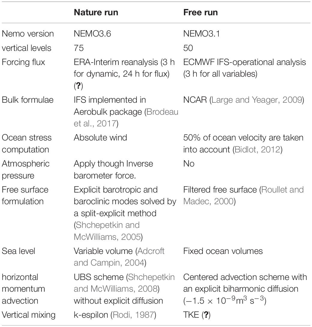
Table 1. Differences in model parameterisation between (NatRun) NR and (Free Run model) FR.

Figure 1 shows the Kinetic Energy (KE) spectrum in three different boxes [(A): Kuroshio Current (130–140°E; 15–25°N); (B): Gulf Stream Current (75–65°E; 25–35°N); and (C): Tropical area (22–11°E; 7°S–7°N)] averaged over the year 2015. For these three regions, NR (black curve) shows more energy at all scales compared to both the other estimates (FR, blue curve and G12, red curve). This difference is more evident in the Gulf Stream and the tropical boxes than in the Kuroshio box. It is also interesting to note that in NR the smallest scales (lower than 100 km), that will be observed by SWOT, exhibit a higher level of energy. These energy differences are mainly due to the numerical choices made for NR: less diffusive, absolute wind, and momentum advection scheme.

FIGURE 1

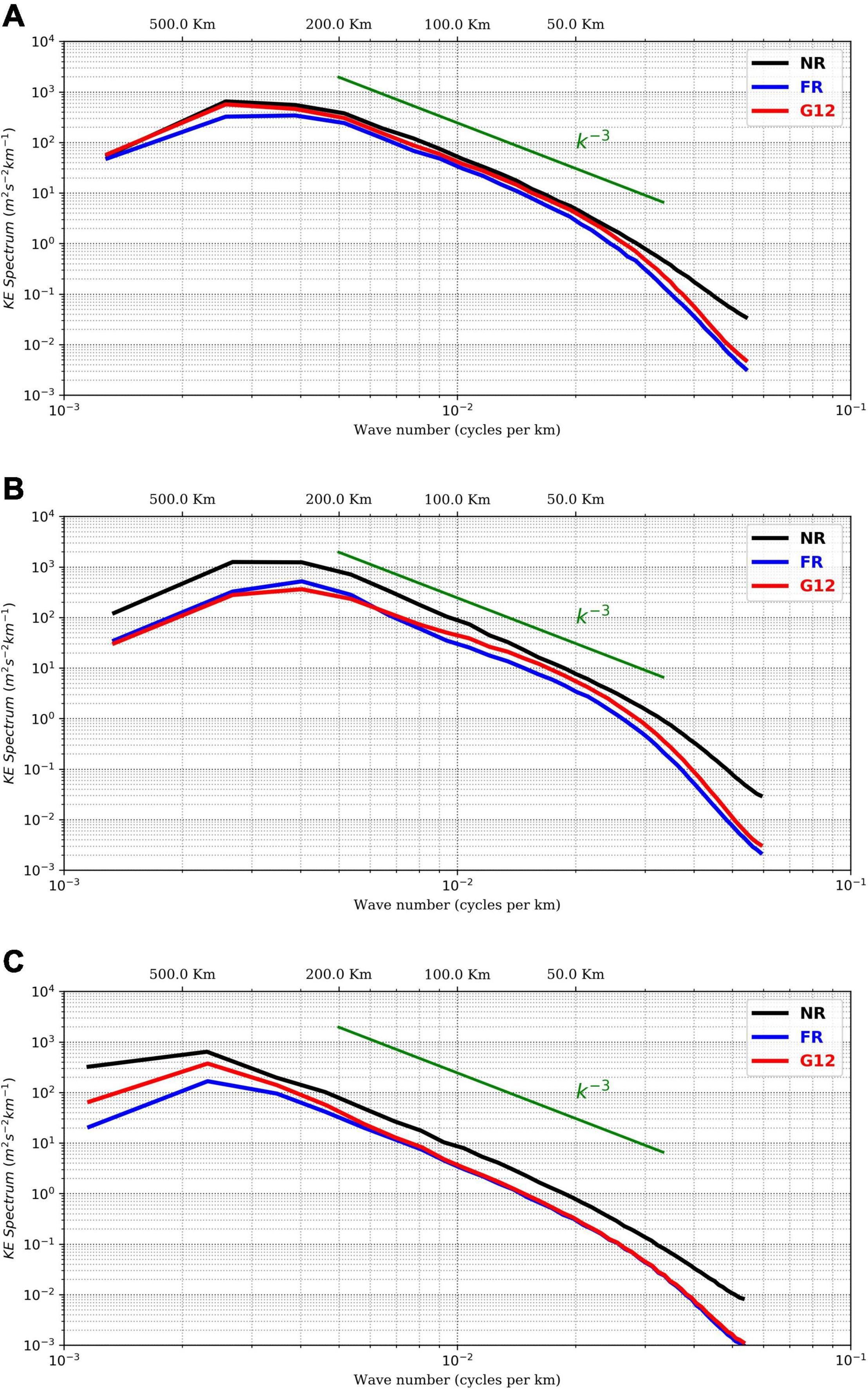
Figure 1. Surface KE (Kinetic Energy, 2015 mean) Spectrum in three panels (A) Kuroshio Current (130–140°E; 15–25°N), (B) Gulf Stream Current (75–65°E; 25–35°N), and (C) Tropic area (22–11°E; 7°S–7°N). Blue curve for FR, red curve for G12, and black curve for NR.

Figure 2 shows the comparison of the 2015 annual SLAs Root Mean Square (RMS) between the NR (panel A), DUACS product (panel B, Ducet et al., 2000; Dibarboure et al., 2011) and G12 (panel C). NR and G12 SLAs were derived by removing the mean sea surface height from the hourly field for each model. All three datasets have comparable magnitudes. The maximum RMS value points in each dataset are located mainly along the fairly well-known major currents (Gulf Stream, Kuroshio, etc.). It is worth noting that the El-Nino signature (present in 2015) is well marked in the three databases. NR does not produce local maxima at exactly the same locations as those observed or simulated with the G12 system, but the global magnitude and the general spatial pattern are consistent with the observations. Otherwise, the Gulf Stream and Kuroshio currents in NR are more spread out where they separate from the continent as compared to the G12 system which assimilates SLA, SST and T/S in-situ profiles.

FIGURE 2

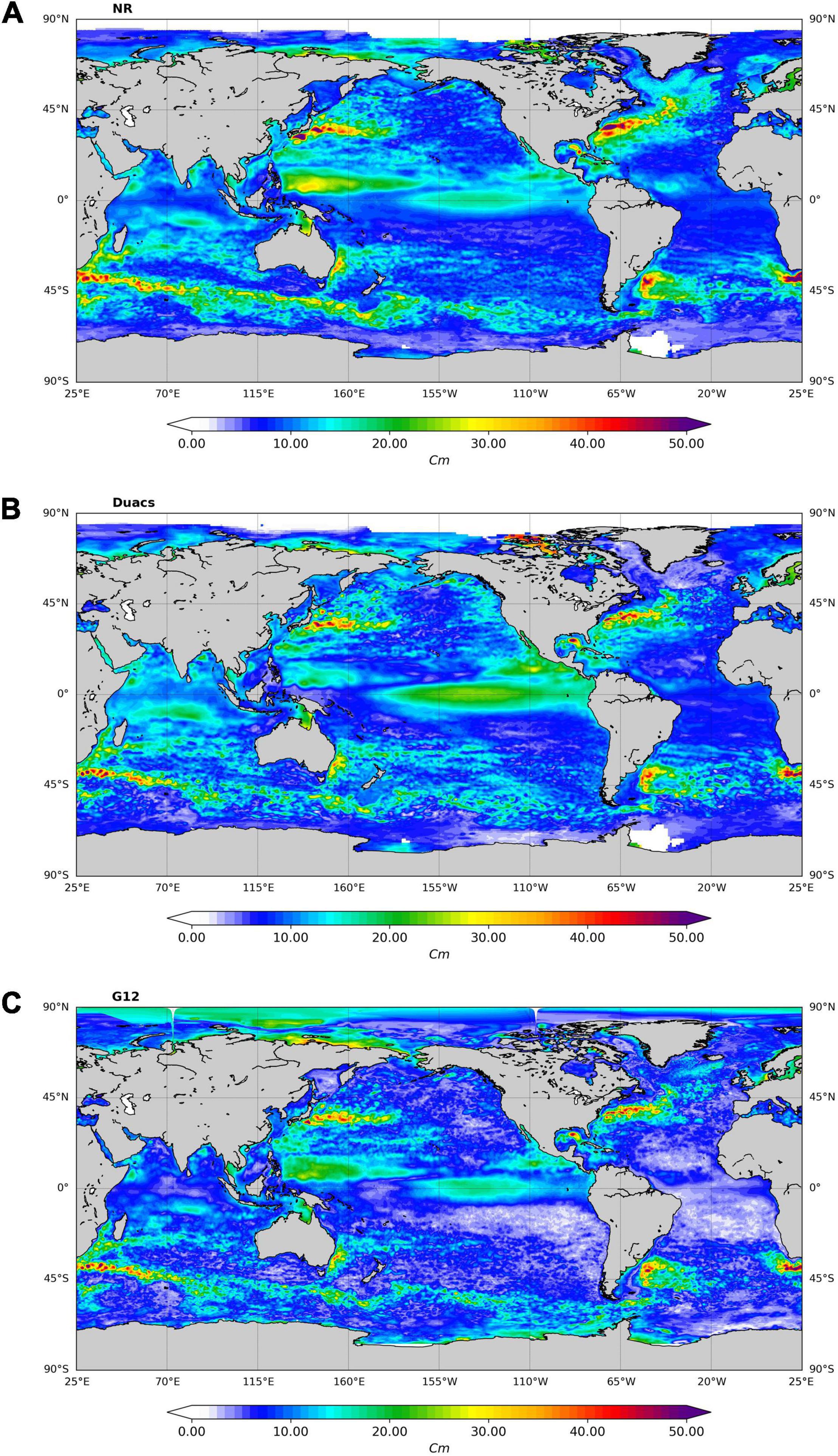
Figure 2. Root Mean Square (RMS) of the sea level anomalies (cm) over 2015: NR (A), Duacs (B), and G12 (C).

Figure 3 shows the evolution over time of the mean temperature between the surface and 100 m in depth. The seasonal cycle of the three fields is in good agreement. The NR (black curve) has a lower temperature compared to FR (red curve) and G12 (blue curve). The difference is stable between NR and G12 (around 0.15°C). On average, FR falls between the other two estimates but with a seasonal variation of the difference: FR is closer to G12 in winter but becomes closer to NR in summer.

FIGURE 3

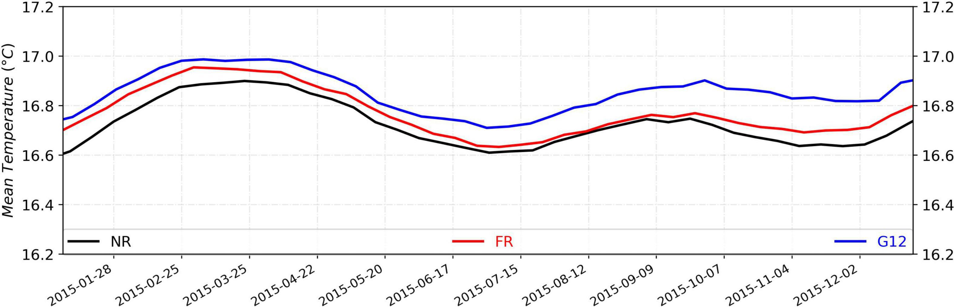
Figure 3. Time evolution of mean temperature between Surface and 100m (°C) area-averaged (black: NR, red: FR, blue: G12).

In Figures 4, 5, the mean and standard deviation of the mixed layer depth (MLD) are compared for two different seasons (March and September). Both in spring and in autumn, NR represents the same signatures as G12, which assimilates realistic data. For example, in March, the NR has a mean MLD of over 250 m in the North Atlantic sub-polar gyre, with strong variability. In September, the mean MLD and its variability are in all respects comparable in the circumpolar current between NR and G12. This is in contrast to FR, which has a MLD that is too deep. This proves the good behaviour of NR, especially with regards to the representation of vertical processes. We can note that the MLD of the NR and G12 are closer to each other than to that of FR.

FIGURE 4

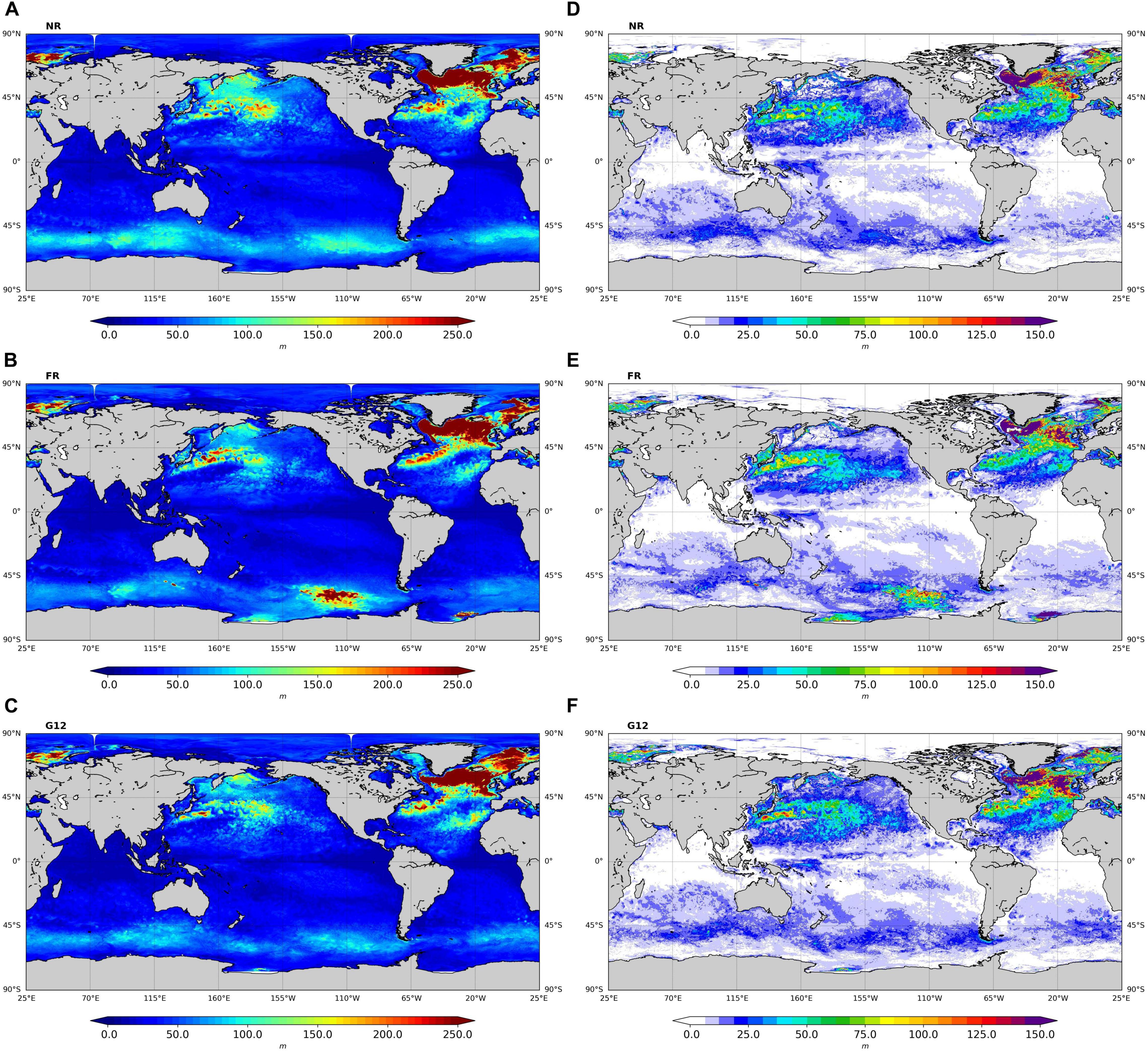
Figure 4. Mean and Standard deviation of the mixed layer depth (MLD, m, March 2015); Mean: NR (A), FR (B), and G12 (C). Standard deviation: NR (D), FR (E), and G12 (F).

FIGURE 5

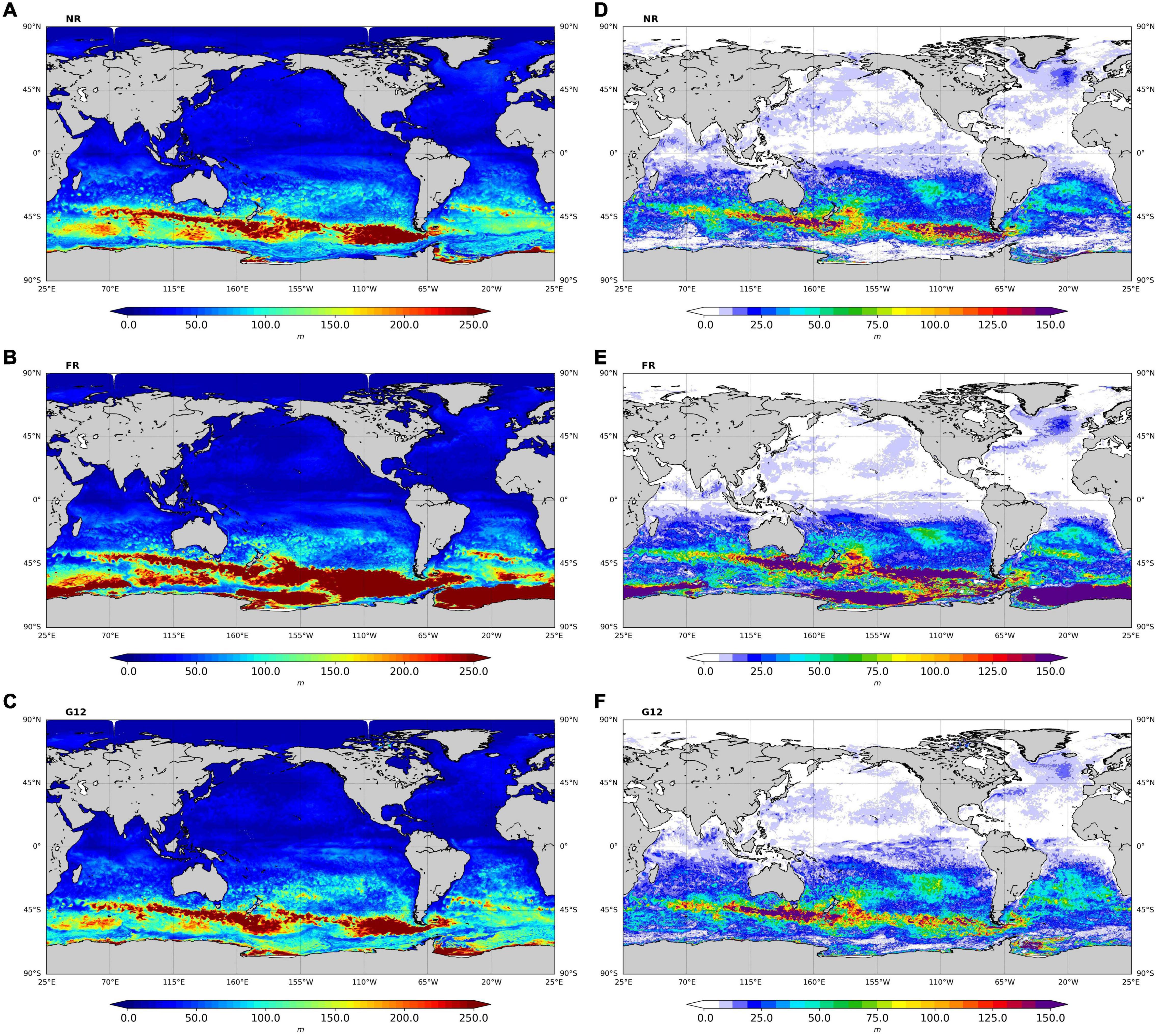
Figure 5. Mean and Standard deviation of the MLD (September 2015); Mean: NR (A), FR (B), and G12 (C); Standard deviation: NR (D), FR (E), and G12 (F).

Simulation of Observations and Noise

All simulated observations were extracted from the NR simulation and these observations were collected over a period of 15 months (from October 1, 2014 to December 31, 2015) which includes the period covered by the OSSEs.

Sea Surface Temperature, Vertical Profiles of Temperature, Salinity, and Ice Concentration

The calculated pseudo surface temperature observations mimic the CMEMS space-time sampling of CMEMS L3S-GLOB-ODYSSEA products. This product merges the collection of sea surface temperature (SST) from multiple satellite sources onto a 0.1° resolution grid over the global ocean. The hourly mean temperature of NR is used to simulate the sea surface temperature observation value. The average SST error is 0.5°C. Finally, it is worth mentioning that the observation errors only depend on the geographical position and not on time. We used the same observation error as the one used in the G12 system (see Lellouche et al., 2013; Lellouche et al., 2018).

The temperature and salinity (T/S) profiles were extracted at the same points and dates as the real in situ profiles observed in 2015 and found in the CORA4.1 database stored in the Coriolis and CMEMS in situ data centre (Cabanes et al., 2013). 3D daily mean temperature and salinity fields from the NR were used to simulate this in situ data. To mimic the instrumental error, the data were perturbed as a function of depth and geographical position with white noise of the order of the standard deviation of the G12 temperature and salinity errors (see Lellouche et al., 2013; Lellouche et al., 2018).

Ice concentration in the Arctic and Antarctic was simulated from NR daily outputs. This pseudo-data respect the spatial-temporal sampling of the CERSAT (Ezraty et al., 2007) products. Our goal was to achieve an OSSE that would be fairly close in terms of observation coverage to our operational systems.

Altimetry Data

Nadir data

The nadir altimetry constellation simulated consists of Jason-3, Sentinel 3A, and Sentinel 3B. The counterparts of the along-track nadir altimeter data were extracted from NR at the 1 Hz frequency corresponding to a spatial resolution of 6–7 km from hourly mean fields of the NR.

Figure 6A shows a snapshot of the NR’s sea surface height (SSH) for the Gulf Stream area, and Figure6B an example of data coverage along the tracks of the three nadir altimeters over 7 days. The coverage appears to be homogeneous over one analysis cycle. This is typical of real-time altimetry sampling.

FIGURE 6

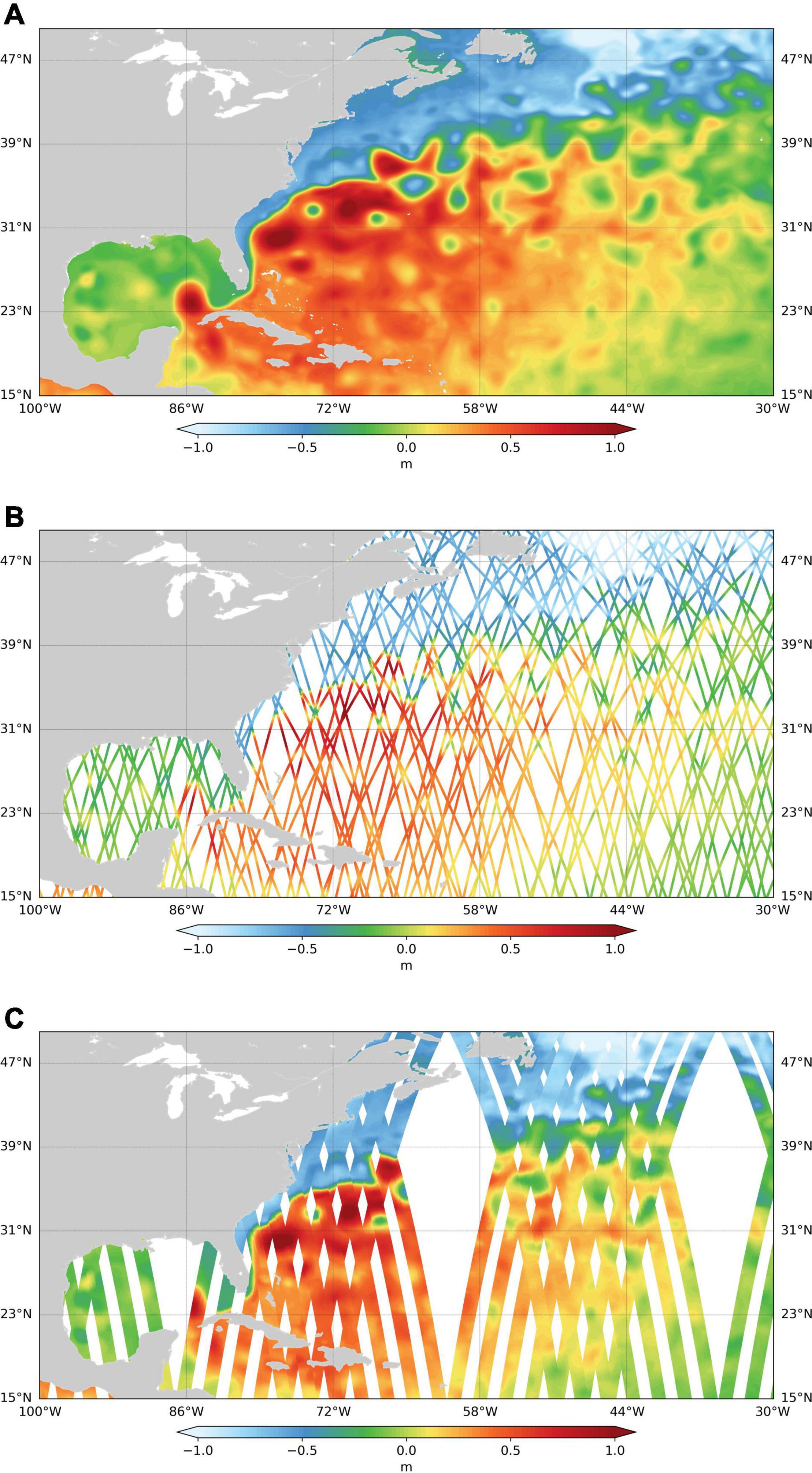
Figure 6. (A) SSH from Truth Run (NR) on January 4, 2015, (B) simulated along-track data from Jason3, Sentinel3A and Sentinel3B for seven days assimilation cycle, and (C) simulated SWOT data (01/01/2015-08/01/2015).

We assumed that the SSH data error does not depend on the distance from the coast. There was no masking of the data in shallow seas. We perturbed the data along the track with white noise of 3 cm standard deviation and did not add any bias.

SWOT data

Surface Water Ocean Topography will provide global SLA observations under a 120 km wide-swath with a middle gap of 20 km. In this study we considered the SWOT data as two-dimensional fields under the swath with a regular along-track and across-track resolution. The pseudo-SWOT observations were simulated from hourly outputs of the NR using the “SWOT Simulator” developed at the Jet Propulsion Laboratory (Gaultier et al., 2016), which is used to generate observations with the expected SWOT sampling and error budget. Along-track and cross-track data extraction depend on both the time position in the along-track direction and the spatial location of the measurement in the cross-track direction. Associated errors were also obtained using the “SWOT simulator” software. The simulator constructs a regular grid based on the baseline orbit parameters of the satellite, namely a 20.86-day repeat cycle, an inclination of 77.6° and an altitude of 891 km and on the characteristics of the radar interferometer on board. In this study, the data were simulated with a resolution of 6 km in both cross-track and along-track directions, which corresponds to the NR and assimilation model grid resolution. Figure 6C shows an example of SWOT data coverage over 7 days.

The SWOT simulator models the most significant errors that are expected to affect the SWOT data, i.e., the KaRIn noise, roll errors, phase errors, baseline dilation errors, and timing errors. It produces random realisations of uncorrelated noise and correlated errors following the spectral descriptions of the SWOT error budget document (Esteban-Fernandez et al., 2017). In our experiments, we only used the KaRIn noise for two reasons: (i) the simulator models the worst expected case and (ii) the observation distribution centres are planning to filter the data from most of these errors. Consequently, as the final error budget is still uncertain and as this was our first effort to assimilate such data in a global model, we preferred to use a more optimistic error budget. The same simulator was used to simulate the nadir data of SWOT.

With a 6 km spatial resolution, the KaRIn noise ranges from 0.2 cm standard deviation in the inner part of the swath to about 0.35 cm on the outer edges of the swath. The standard deviation of the KaRIn noise also depends on the significant wave height (SWH) parameter which is a value between 0 and 8 m. In our study, the simulator was set up with a constant SWH = 2 m. An example of simulated data along a swath is shown in Figure 7. Panel A shows the “truth” and panel B the “truth” corrupted by the KaRIn noise. Finally, panel C shows the spatial structure of the noise and the standard deviation of the errors is shown in panel D. Figure 7E shows the standard deviation of the KaRin random error considering across-swath resolutions of 1 km (solid line) and 6 km (dashed line) as a function of the cross-track distance in km.

FIGURE 7

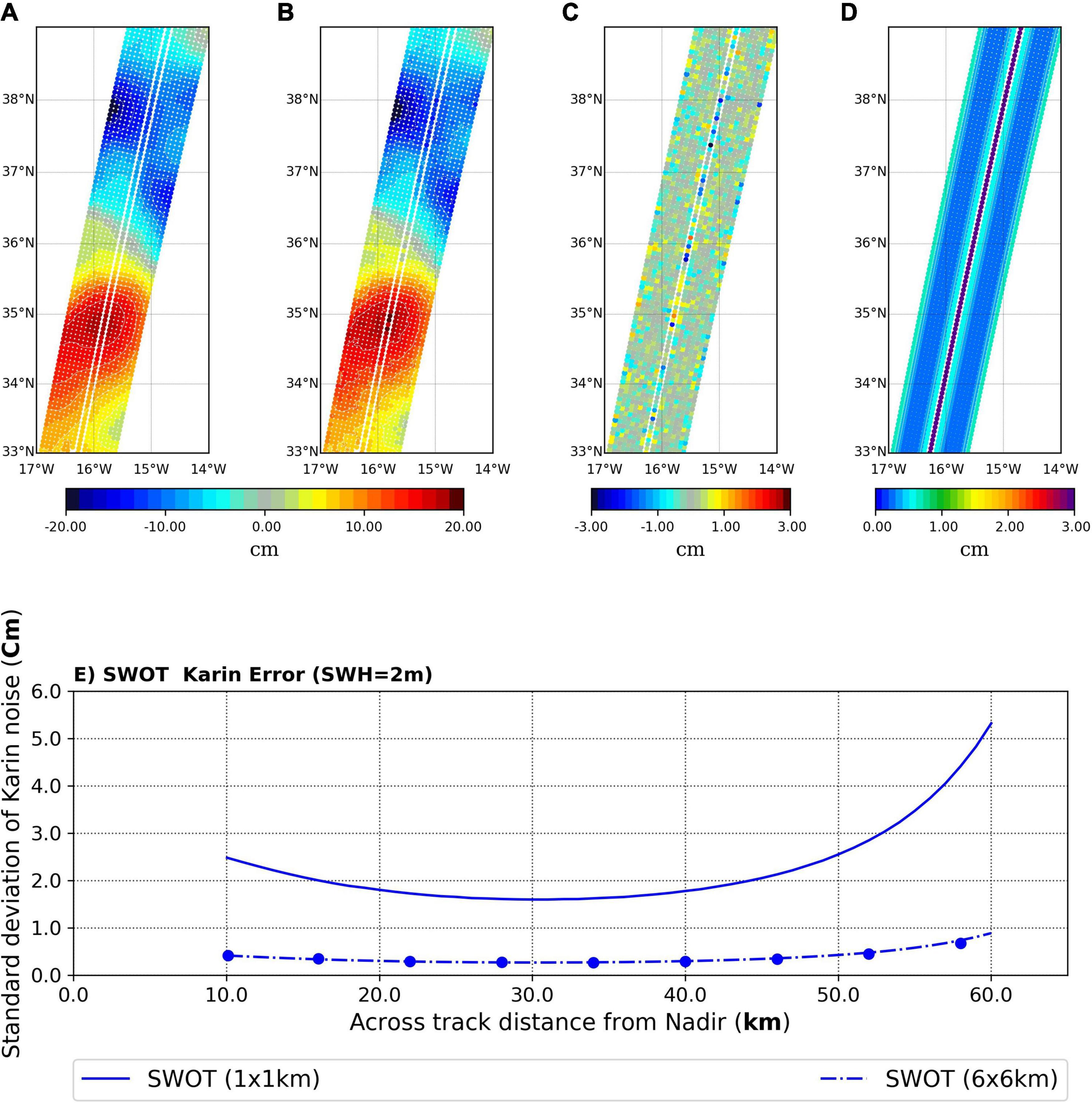
Figure 7. Example of SSH pseudo-observation along a SWOT swath: (A) Pseudo-observation, (B) Pseudo-observation + noise (KaRin noise), (C) KaRIn noise along swath, and (D) standard deviation of the KaRIn noise. (E) The curves displayed show the Swot instrumental error with SWH = 2 m (wave height), considering across-swath horizontal resolution of 1 km (solid line) and 6 km (dash line).

Observation Operator and Error Variances

In the data assimilation scheme, the computation of the innovation requires defining an observation operator to compute the model counterpart which is equivalent to the observations. We describe here the observation operators used for the OSSEs that assimilate the pseudo-observation simulated from the NR.

The model equivalent to SSH and SST observations was calculated by interpolating the model fields onto the observation space using a bi-linear interpolation in space, and a linear interpolation between the nearest model time steps. For the T/S profiles, the model was interpolated at the observation locations, and then a spline was adjusted to the observed profile to calculate the innovations (observations minus model forecast) at the level of the vertical grid of the assimilation model.

In the data assimilation system, the observation error covariance matrix was assumed to be diagonal. It is prescribed a priori as a sum of an “instrumental” error, depending only on the observation type and location, added to a representativity error. The latter represents the part of the observed signal in the observations that the model is not able to represent, due to its resolution or because of missing processes in the model equations. Since the model configuration chosen for the OSSE differed from the NR configuration, from which the pseudo-observations were extracted, a representativity error was also taken into account in observation errors for the OSSEs.

The instrumental errors specified in the assimilation scheme are consistent with the simulated noise for each data set extracted from the NR. For SSH observations, an error of 3 cm for the nadir was prescribed, for SWOT the error (KaRin) is shown in Figure 7C and for SST an error equal to 0.5°C was prescribed.

For the altimetry (nadir and SWOT), in addition to the observation error, we used an SSH representativity error. Figure 8 shows this representativity error for the SSH observations that were calculated from the standard deviation of the NR SSH for scales smaller than 100 km. For SST, the representativity error was prescribed as a map constant in time as in the global 1/12° system presented in Lellouche et al. (2018).

FIGURE 8

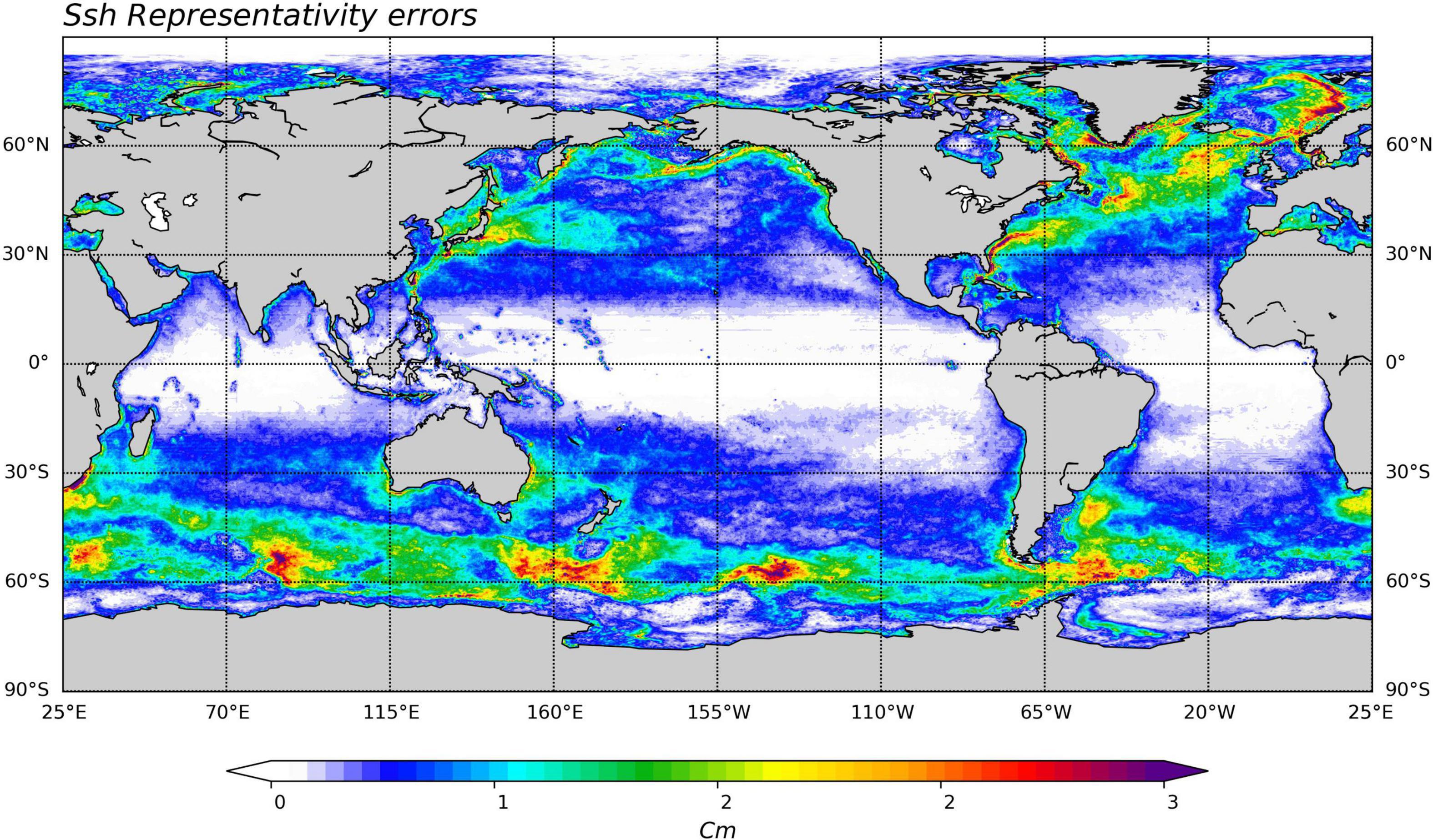
Figure 8. SSH representativity error (cm).

The Assimilation System

The assimilation system is the system used to perform the OSSEs. It consists of a physical ocean model and an assimilation scheme which has been modified to serve the OSSEs (see section “Data Assimilation Scheme”). The simulated observations described in the previous section were assimilated in this system.

Ocean Model Configuration

The FR ocean model configuration was also based on a global 1/12° resolution configuration but with only 50 vertical levels (1 m at the surface to 450 m at the bottom). This configuration was also based on an older NEMO version (version 3.1; Madec, 2008). This assimilation model configuration shares many parameters with the NR. Nevertheless, the two model configurations differ in several respects, thus ensuring a level of difference between simulations comparable to those between the model and the observations. The main differences between this ocean model configuration and the NR are summarised in Table 1.

All these differences in model parameterisation led to the simulation of two different ocean states and ensured that the RMSE difference between the simulations was comparable to that between the model and the observations. As shown in section “Nature Run and Simulated Observations,” in most of the cases, the choices made for NR simulation (absolute wind, UBS scheme, split-explicit free surface, atmospheric pressure forcing) induced a higher energetic level than in the OSSEs.

Data Assimilation Scheme

The data assimilation system (SAM: Système d’Assimilation Mercator) used for current Mercator Ocean International (MOi) operational systems has already been described in Lellouche et al. (2013, 2018). It consists of a 3D-Var bias correction for the slowly evolving large-scale biases in temperature and salinity, and a local version of a reduced-order Kalman filter based on the Singular Evolutive Extended Kalman Filter (SEEK) formulation introduced by Pham et al. (1998). Several previous OSSEs (Gasparin et al., 2018; Verrier et al., 2018; Hamon et al., 2019) including some related to Swath observations (Bonaduce et al., 2018), used this system.

In this section, we recall the main particularities of both the SEEK and 3D-Var methods. The focus is on the changes made to improve the SEEK’s performance in the OSSEs described here. First, we present a 4D extension of the data assimilation method described in Lellouche et al. (2013). It will be part of the future global MOi operational system to be deployed in the CMEMS portfolio (Le Traon et al., 2019) by the end of 2021. Second, changes in the construction of the required background error covariance matrix are described in detail along with some results showing the impact of these changes.

To present the improvements made in our system, let us first introduce the Kalman filter analysis step as:

$$\delta {\mathbf{\text{x}}}^a={\mathbf{\text{PH}}}^T{\left({\mathbf{\text{HPH}}}^T+\mathbf{\text{R}}\right)}^{-1}\mathbf{\text{d}}(1)$$

where δx^a is a vector of analysis increments (correction) of the size of the state vector m, d is the innovation vector of size o (observations minus forecasts in the observations space), P and R are the background and observation error covariance matrices of size m×m and o×o, respectively, and finally H is the so-called observation operator mapping the state vector from the model space to the observation space with ()^T the transpose operator.

The specificity of the SEEK filter is the use a low-rank approximation of the background error covariance matrix P. In this case, we write P = SS^T, where the matrix S, also called the anomaly matrix, has many more lines m–(size of the state vector) than columns n. When n is much smaller than the number of observations and R is diagonal, the Eq. 1 can be written in a numerical efficient form as (Brankart et al., 2009):

$$\delta {\mathbf{\text{x}}}^a=\mathbf{\text{Sw}}(2)$$

with the vector w given by:

$$\mathbf{\text{w}}={\left[\mathbf{\text{I}}+{\mathbf{\text{Y}}}^T{\mathbf{\text{R}}}^{-1}\mathbf{\text{Y}}\right]}^{-1}{\mathbf{\text{Y}}}^T{\mathbf{\text{R}}}^{-1}\mathbf{\text{d}}(3)$$

where I is the identity matrix and Y = HS is the anomaly matrix in the observation space.

Equation 2 reveals that the increment is a linear combination of the columns of S. Therefore, the set-up of S is a critical point to the system’s performance. For this reason, the next sections give a detailed presentation of how this matrix in constructed in MOi SAM system for 3D and 4D formulations of the assimilation problem. Sections “Constructing the State Anomalies” details how we construct the anomalies composing the columns of S using a climatological run, and section “From 3D-FGAT to 4D-FGAT” provides a detailed description of the approximation of S in the 3D and 4D formulations.

Before entering the details, it is worth citing two essential aspects of the MOi analysis system: a localisation scheme and an adaptativity technic. MOi system apply a local analysis scheme (Ott et al., 2004; Hunt et al., 2007; Lellouche et al., 2013). It means the Eqs 2 and 3 are solved independently for each model point, and the analysis considers only observations lying within a prescribed distance from the analysed point. A Gaussian function weights the observations increasing their error as a function of their distance from the analysed point.

The used distance in the analysis scheme is twice the local spatial correlation scale estimated using a previous global reanalysis (see details in Lellouche et al., 2013). In our global configuration, the spatial correlation scale, defined as the distance where the correlation coefficient equals 0.4, is about 100 km (250 km at the equator). The size of the local region (i.e., the correlation scale) is essential because (i) it reduces sampling noise in the background covariance matrix and (ii) it controls the regularity of the increment by inserting more or fewer observations in each local analysis. The degree of smoothness of the analysis depends on the number of available observations, the dimensionality of the sampled dynamics, and the rank of the localised covariance matrix.

The adaptativity technic is based on the work of Desroziers and Ivanov (2001) and aims to find a scalar α for each local region, that multiplies the local restriction of P, so that the following equation is satisfied for each local region and each analysis cycle:

$$\alpha \times tr\left({\mathbf{\text{HPH}}}^{\text{T}}\right)+tr\left(\mathbf{R}\right)=tr\left({\mathbf{\text{dd}}}^{\text{T}}\right)(4)$$

where tr(A) is the trace of A. This step is crucial for our analysis scheme since it compensates for the lack of information about the variance of the forecast error in the construction of the background covariance matrix.

The analysis increment is injected into the model using the so-called Incremental Analysis Update (IAU) method (Bloom et al., 1996; Benkiran and Greiner, 2008). This consists of adding at each time step of the physical model the increment weighted by a function. The weight is a piecewise function of time such as its time integral over the DAw equals one (Lellouche et al., 2013). The IAU in the 4D case (4D-IAU; Lei and Whitaker, 2016) uses a time interpolation in between calculated increments and weights the resulting increment at each model time step by a piecewise function as in the 3D case. It should be noted that when only one increment in the assimilation window is calculated, the 4D-IAU is the same as the 3D-IAU.

In practice, the SAM system is a sequential scheme composed of a forecast step, followed by an analysis step. Here, we use a 7-day assimilation window because this set-up is used in MOi operational systems. During the model integration, the innovations are calculated at the right location and at the right time. After each analysis, the data assimilation produces increments of SSH, T, S, zonal velocity (U) and meridional velocity (V). All these increments are applied progressively in the hindcast run using the IAU method.

Constructing the State Anomalies

This section details the construction of the collection of anomalies δx used to build the matrix S. The general idea is to calculate an anomaly as the difference between a model field at a given time and an averaged field mimicking an ensemble mean (Lellouche et al., 2013). The anomalies generated by this method must cover the forecast error subspace as well as possible. In the current MOi analysis systems using the 3D scheme, the anomalies come from a climatological run (without assimilation) that is long enough to ensure the model has visited a large portion of the state space. In this study, we use a sharper filtering in space and the anomalies come from the reanalysis (with assimilation). Next, a step-by-step recipe on the anomaly construction is given.

The anomalies are constructed in three steps:

(1) Each 24 h-average daily output of a long climatological run is spatially smoothed using a Shapiro filter to cut-off scales that are shorter than a prescribed wavelength ${\omega }_k^{-1}$. The 24h-average condition may be relaxed if the assimilation is intended to correct high frequency signals.

(2) The spatially filtered time series produced in (1) is time filtered using a low-pass Hanning filter with a cut-off frequency of ω_f.

(3) We subtract from each daily output generated in (1) the corresponding low-passed field generated in (2). At this step, we obtain a series of model states which are characterised by periods longer than one day and shorter than ${\omega }_f^{-1}$, and with spatial features with wavelengths greater than ${\omega }_k^{-1}$. One should note that the time filtering probably acts on the entire wavenumber domain, reducing the energy for wavelengths that are longer than the cut-off scale.

Therefore, for a given climatological run, two parameters ω_k and ω_f, control the anomalies’ information content. The first one reduces the energy contained in small wavelengths that are not well observed by the observational network. The second parameter selects the corresponding time scales of the features corrected during the assimilation step. One important aspect of this methodology is that most of the seasonal-to-interannual signals are removed from our anomalies. This avoids trying to correct forecast errors that are predominantly at the mesoscale with inadequate anomalies. This procedure is essential for the deep ocean, for which there are almost no observations, and all corrections are based on the covariance between the observed variables of the state vector and the non-observed variables.

Some tests (not shown) were performed by varying ω_k and ω_f to find a set of parameters maximising the spectral energy in the band of 50-250 km. The retained values are 21 km for ${\omega }_k^{-1}$ and 48 days for ${\omega }_f^{-1}$. The values used by the current global high-resolution CMEMS GLORYS12 reanalysis (Lellouche et al., 2021) are 64 km and 24 days. As a consequence, the current CMEMS system retains a narrower spectral band. Next, two different anomaly bases were calculated to demonstrate the impact of changing these parameters. These two bases use 8 years of the CMEMS ocean reanalysis as the climatological run. We call “new basis” the one using the couple (21 km, 48 days) and “old basis” the one using (64 km, 24 days).

Figure 9 shows the power spectral density of the anomalies calculated for the Sea Level in the Kuroshio region (150.0–162.0°W, 30.0–42.0°N) for the new basis (red curve) and the old basis (black curve). The new filtering parameters produce very different repartition of energy. The new basis has more energy at all scales compared to the old one. Its shape is also different, with a flatter spectrum for the 250–50 km band. The cyan-coloured curve in the figure represents the typical nadir observation error (3 cm). In a Kalman filter scheme, the ratio between background error and observation error determines the weight given to each piece of information. The crossing point between these spectra determines the wavelength for which background and observations have the same weight in the analysis. In the given example, large scales are more effectively constrained by the observations. Using the crossing point as a reference to well-constrained wavelengths, we have a gain of about 50 km compared to the old background error covariance.

FIGURE 9

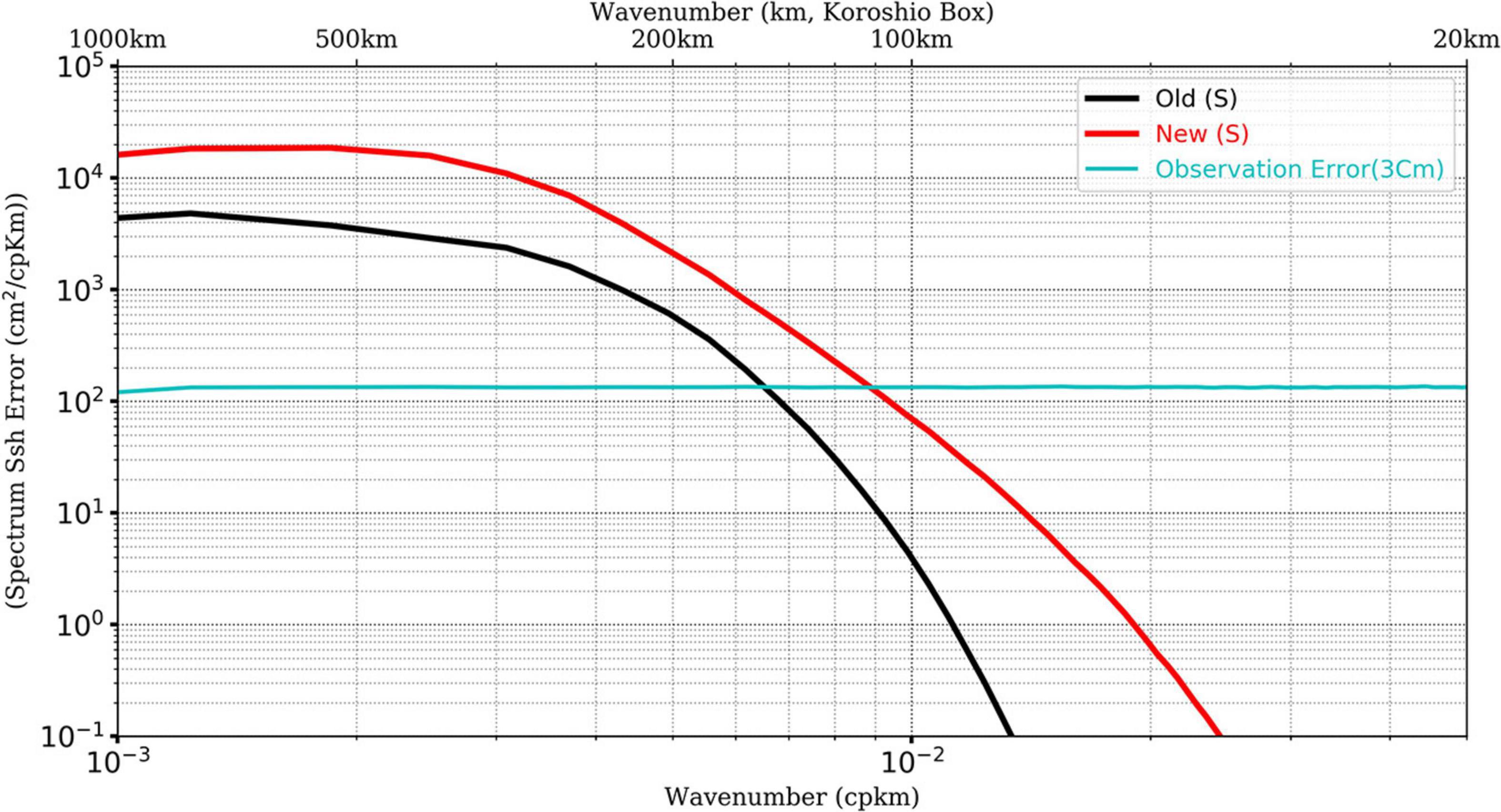
Figure 9. The power spectral density of the anomalies calculated for the Sea Level (cm²/cpkm) in the Kuroshio region (150–162°W, 30–42°N, the black box in the Figure 12A), for the new basis (red curve) and the old basis (black curve), cyan curve is observation error. Spectrum are average in time and space.

It is worth recalling that before the assimilation step, Eq. 3 is used to inflate the covariance matrix. It is equivalent to multiplying the spectrum in the figures by a scalar. Since the large-scale signals dominate the variance, the inflation is never sufficient to extend the impact of the assimilation towards high wavenumbers, as much as one might desire this in the case of high-resolution data. For example, one cannot obtain the new spectrum by simply multiplying the old one by a scalar. Thus, the most important change between the old and the new versions is the shape and relatively higher energy in the new version’s mesoscale range. In section “Impact of the Improvements of the Background Error Covariances,” we present data assimilation experiment results using both bases to demonstrate how the new basis indeed improves the assimilation scores.

From 3D-FGAT to 4D-FGAT

This section presents how the anomaly matrix S is constructed for the 3D and 4D. The reader will find which anomalies are used in each update step and how Eqs 2 and 3 are modified accordingly to each formulation.

For both formulations, the MOi systems follow the First Guess at Appropriate Time (FGAT) strategy to compute the innovations d (observations minus model background) in the data assimilation window (DAw):

$$\mathbf{\text{d}}=vec\left({\mathbf{\text{y}}}_j-{\mathbf{\text{H}}}_j\mathbf{\text{x}}_j^f{}_{j\in J}\right)(5)$$

where J is the set of indexes for which observations are available at time t_j, for t_j inside the DAw. y_j is a vector composed by all observations at time $t_j,{\mathbf{\text{H}}}_j{\mathbf{\text{x}}}_j^f$ is the so-called model equivalent at the right time with H_j the operator that maps the state vector x_j from the model space to the observation one. The operator vec () gathers all vectors, thus preserving the number of columns.

3D-FGAT

The 3D scheme aims to identify the best model state, in the Kalman sense (Gelb et al., 1974), at an instant in time, given all observations in the DAw. In the MOi data assimilation system, the analysis is done for ${\mathbf{\text{x}}}_c^f$ at the center of the assimilation window and the associated matrix of anomalies S_cis constructed using a collection of predefined daily anomalies (δx) corresponding to a time window (L = ± 45 days) around the reference day t_c. The way these anomalies are constructed was described in the previous section. To be more precise about which anomalies are used by the analysis, let us define a set of indices I:

$$I=\{i\in [-L;L]|mod(i,s)=0\}(6)$$

with s a sampling frequency and mod the modulo operation. For each year k of the climatological simulation an anomaly matrix is defined as:

$${\mathbf{\text{S}}}_c^k=mat\left(\delta \mathbf{\text{x}}_{c+i}^k{}_{i\in I}\right)(7)$$

with mat an operator gathering vectors or matrices and preserving the number of lines. The matrix ${\mathbf{\text{S}}}_c^k$ has the dimension of the state vector as the number of lines and the number of columns equals the cardinality of the set I given by the Eq. 6. The final anomaly matrix used in the analysis equation is written as:

$${\mathbf{\text{S}}}_c=mat\left(\mathbf{\text{S}}_c^k{}_{k\in [1..K]}\right)(8)$$

where K is the number of years in the climatological basis. Therefore, S_c has the same number of lines as ${\mathbf{\text{S}}}_c^k$ and K times its number of columns, i.e., K×card(I) columns. Figure 10 represents a simplified scheme about the construction of the matrix S_c for the cases K = 1,L = 3, and s=1. Note that in this case Eq. 8 resumes to Eq. 7. In this simple case, I = {−3,−2,−1,0, + 1, + 2, + 3} and the anomaly matrix has seven columns (represented by red squares in the figure). Note that all anomalies are considered to be at time c even though their time stamp varies from c-3 to c+3.

FIGURE 10

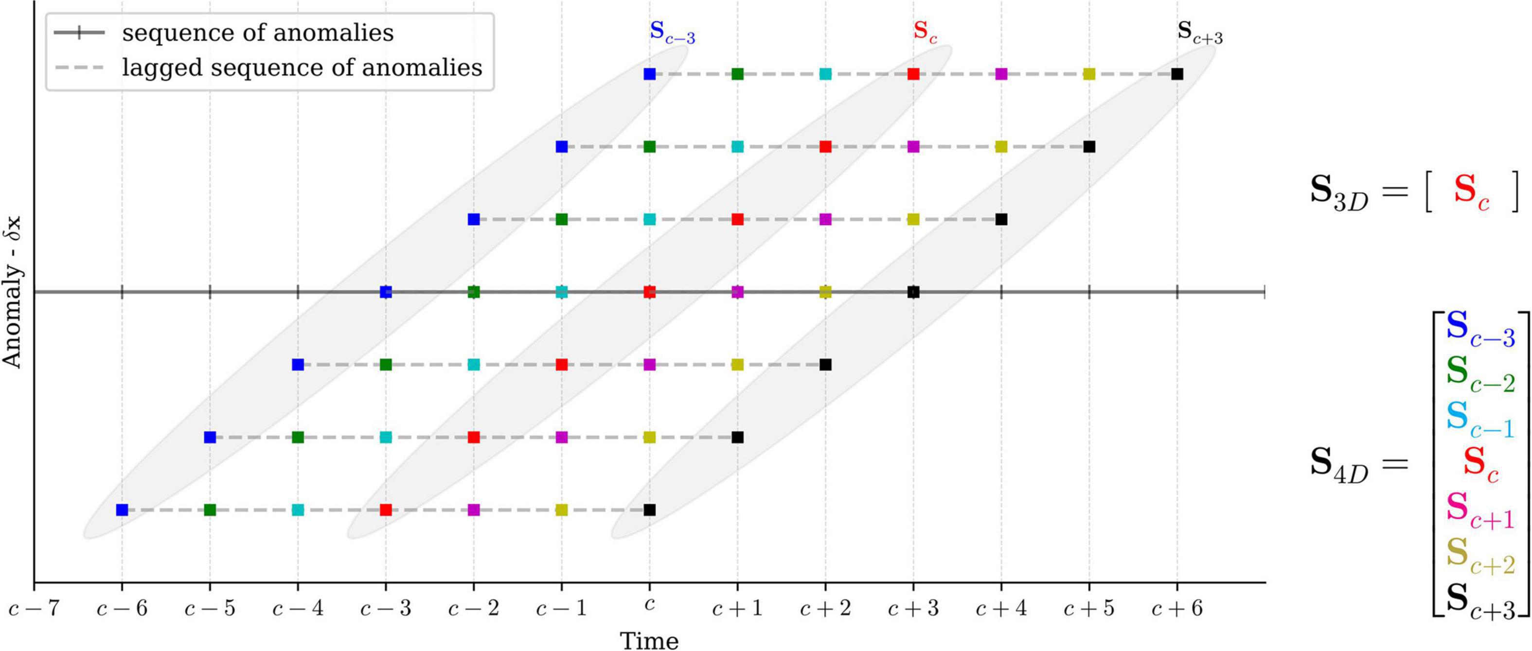
Figure 10. Schematic construction of the anomaly matrix S for the 3D and 4D analysis scheme. Colours represent the days within the DAw. Shaded ellipses represent the anomaly matrices for days c-3, c and c+3. “Lagged sequence of anomalies” (dotted lines) were displaced in the vertical axis with respect to the “sequence of anomalies” (full line) for visualisation purpose. The S_4D covariance matrix corresponds to the S_3D matrix augmented with past and future anomaly matrices. Their number of columns is the same.

It is worth noting that there are L anomalies missing at the beginning of the first year (k = 1) and at the end of the last year (k = K). For years 1 < k < K the used boundary conditions are:

$$\{\begin{array}{c}\hfill \delta {\mathbf{\text{x}}}_{c+1}^k=\delta {\mathbf{\text{x}}}_{N-(c+i)}^{k-1};\forall i\in I,c\in [1,N]|c+i<1\hfill \\ \hfill \delta {\mathbf{\text{x}}}_{c+1}^k=\delta {\mathbf{\text{x}}}_{c+i-N}^{k+1};\forall i\in I,c\in [1,N]|c+i>N\hfill \end{array}(9)$$

with N the number of available anomalies in one year. Eq. 9 ensures time continuity of the series of anomalies from one year to another.

Then, with the background anomaly matrix at hand an increment, or model correction, is calculated using Eqs 2 and 3:

$$\delta {\mathbf{\text{x}}}_c^a={\mathbf{\text{S}}}_c\mathbf{\text{w}}(10)$$

where:

$$\mathbf{\text{w}}={\left[\mathbf{\text{I}}+{\mathbf{\text{Y}}}_c^T{\mathbf{\text{R}}}^{-1}{\mathbf{\text{Y}}}_c\right]}^{-1}{\mathbf{\text{Y}}}_c^T{\mathbf{\text{R}}}^{-1}\mathbf{\text{d}}(11)$$

and

$$\{\begin{array}{c}\hfill {\mathbf{\text{Y}}}_c=vec\left({\left\{{\mathbf{\text{H}}}_{\text{j}}{\mathbf{\text{S}}}_c\right\}}_{j\in J}\right)\hfill \\ \hfill R=diag\left({\left\{{\mathbf{\text{R}}}_j\right\}}_{j\in J}\right)\hfill \end{array}(12)$$

with Y_c the anomaly matrix in the observation space at the centre of the DAw. The operator diag( ) creates a block diagonal matrix. In our case, R_{j ∈ J} are all diagonal matrices and therefore diag( ), concatenates all diagonal entries in the diagonal of R.

Hence, Eq. 10 explicitly shows that the increment is indeed a linear combination of the columns of the anomaly matrix, where the coefficients in w are a function of the background error covariance matrix in the observation space at time t_c, the observation error covariance matrix, and of the innovation vector.

It is essential to note that the H operator in Eq. 5 applies to x at the same time instance t_j while in Eq. 12 each H at time t_j applies to the same S at time t_c. This means that the first operator takes into account the time while the second takes into account the spatial position of the observation. As a consequence, the observed dynamics that evolve significantly within the DAw may not project well onto Y_c. As an example, a typical phase speed of sea surface height signals at the equator is of the order of 1 m/s (Schouten et al., 2005). Consequently, in a 7-day DAw these features may propagate over 600 km.

Three parameters control the number of anomalies used in the analysis: the size of a local window L, the sampling frequency s and the number of years in the climatological run K. In the OSSE presented in this article, L = 45 days, and the sampling frequency is s = 2 days. This set-up avoid taking the entire sequence of anomalies (s = 1) because they may have a high degree of collinearity. The number of years available from the climatological run is K = 8. With this setting, the cardinality of I is 45 and, hence, one analysis step uses K × I = 360 anomalies.

4D-FGAT

The 4D-FGAT scheme aims to identify the best model trajectory in the assimilation window given all observations in the DAw. This means that a collection of increments is now calculated. In this case the innovations are still being calculated according to Eq. 5 and in addition one anomaly matrix is specified for each time an observation is available. The scheme is similar to the asynchronous ensemble Kalman filter described in Hunt et al. (2007). What is described next is how the 4D covariance matrix is approximated in this case.

As described in the previous sections, the anomaly matrices are constructed using Eqs 6–9. In the 4D scheme, N_daw matrices like Eq. 8 are used. N_daw varies according to the catalogue of anomalies previously constructed. If for example the catalogue contains daily anomalies, as in our case, and DAw is seven days length, then N_daw = 7. Hence, the Eq. 8 is used to build 7 anomaly matrices: S_c−3,S_c−2,S_c−1,S_c,S_{c + 1},S_{c + 2,}S_{c + 3}, the subscript c recalling that c refers to the centre of the DAw. The Figure 10 presents a schematic view of the anomalies used in the 3D and 4D scheme for the specific case where daily anomalies are considered, and L = 3, s = 1, and K = 1. Each colour represents one anomaly, i.e., one column of S. Shaded ellipses represent the anomaly matrix for each day in the 4D scheme. The anomalies in this case are time-lagged anomalies’ trajectories. Note, that at time c the 4D and 3D matrices are the same.

The 4D scheme allows a better approximation of the anomaly matrix. The hypothesis is that this sequence of anomaly matrices contains information about the model dynamics for the scales we want to correct, such as for example the propagation of mesoscale or wave features. The increments can be written as:

$$\delta {\mathbf{\text{x}}}_i^a={\mathbf{\text{S}}}_i\mathbf{\text{w}},i\in I_{Ndaw}(13)$$

where the set I_Ndaw has N_daw elements and defines the time instances for which anomalies are available in the DAw. The weights w given by:

$$\mathbf{\text{w}}={\left[\mathbf{\text{I}}+{\mathbf{\text{Y}}}^{\text{T}}{\mathbf{\text{R}}}^{-1}\mathbf{\text{Y}}\right]}^{-1}{\mathbf{\text{Y}}}^{\text{T}}{\mathbf{\text{R}}}^{-1}\mathbf{\text{d}}(14)$$

$$\mathbf{\text{Y}}=vec\left(\widehat{{\mathbf{\text{H}}}_j}\mathbf{\text{S}}_l{}_{j\in J,l\in N_{daw}}\right)(15)$$

where $\widehat{\mathbf{\text{H}}}= \mathbf{\text{HT}}$, with T interpolating S from the instant at which anomalies are available inside the DAw to times when observations are available. We see that now the observation operator is applied to the anomaly matrix at the right time. Note that each increment uses the same weight, i.e., w is constant in the DAw.

The increments calculated at the centre of the DAw for the 3D and 4D methods lie in the same subspace; they are the linear combination of the same set of anomalies. Differences are due only to the weights given to each direction (or anomaly). Therefore, this 4D method does not necessarily increase the rank of error subspace. The advantage of this method is that the information about the time evolution of the system contained in the innovation vector d is projected into an ensemble of model trajectories.

In this way, the weights in w reflect which anomaly trajectories best explain the innovation trajectory weighted by the observation error (matrix R).

The 4D method may, consequently, improve the ocean dynamics with significant evolution in the DAw. They are notably fast wave dynamics and the advection of mesoscale/submesoscale features in high energetic regions. Of course, the efficiency with which these dynamics are constrained by the assimilation depends on the observation network and on the information contained in the S matrix.

Bias Correction Scheme for Large-Scale 3D Temperature and Salinity

A 3D-Var bias correction (BC) has been applied for temperature and salinity fields in MOi systems since 2009. It was first described in Lellouche et al. (2013). It has been also used for satellite sea surface salinity in Tranchant et al. (2019). The aim of BC is to correct the large-scale, slowly-evolving errors of the model, whereas the SEEK assimilation scheme is used to correct the smaller scales of the model background error. Spatial correlations are modelled by means of an anisotropic Gaussian recursive filter (Wu et al., 1992; Purser et al., 2003; Farina et al., 2015). This is applied separately to the model’s prognostic temperature and salinity equations from in situ profile innovations calculated over the preceding month on a 1° × 1° coarse grid. Finally, BC increments of temperature, salinity and dynamic height are computed and interpolated on the model grid and applied as tendencies in the model prognostic equations with a 1-month timescale.

This early version had shortcomings. For instance, the correlation radii were still constant for the whole area, at all levels, with just an anisotropy of a ratio of 3 at the equator. A study of the flaws of the system showed that the structure of the estimated bias was too zonal near the equator. The recent reanalysis at G12 covers the Argo period. It was therefore possible to use an extended period (2004–2016) to estimate the correlation radii. A first result was to reduce the anisotropy to a ratio of 1.5 at the equator. It was also possible to estimate constant but different zonal and meridional radii of correlation per level. The G12 innovations were used to estimate the large-scale radii of the bias. A common profile was deduced for temperature and salinity.

The main difficulty of this task is to estimate regionally the large-scale radius of the bias from the innovations in the system, free from the observation error and mesoscale. We were only interested in the radius of the large-scale bias, because SEEK takes the mesoscale into account very well via the anomalies. We used a revised version of Hollingworth and Lonnberg’s method (1986), which seeks to represent the covariances as a function of the separation distance by a Gaussian.

The sum of a Gaussian for the meso-scale (MS) and a cardinal sinus [sinus(x/L)/x] for the large scale (LS) was therefore sought in order to model the covariances. Figure 11 is typical of the equator where there is no MS but equatorial waves: the MS radius is ∼200 km and nearly 600 km for the LS radius, the bias being important. The covariance as a function of the separation distance is shown in black. The Gaussian in orange is the one that best approximates the MS error. The decay beyond the MS zone is much slower than a Gaussian shape (“fat tail”). This decay is approached by a cardinal sine whose characteristic length is ∼1,000 km. The bias is sharp enough to be identified and modelled, and the approximation of the covariance (the sum MS + LS in green) is good.

FIGURE 11

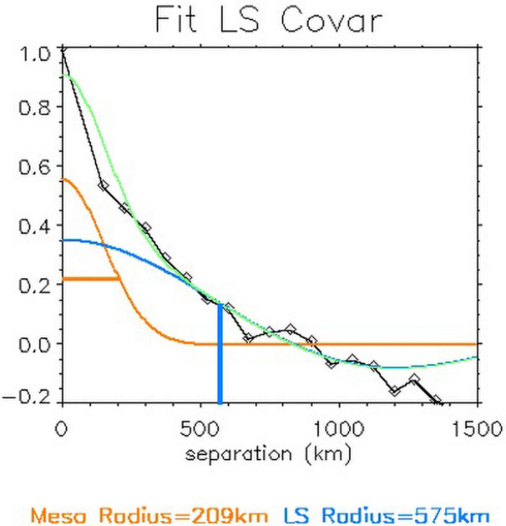
Figure 11. The covariance as a function of the separation distance is shown in black. The Gaussian in orange is the closest approximation to the mesoscale error; the cardinal sine in blue is the approximation to the large-scale error; the covariance approximation (the sum MS+LS) is in green.

This was done for the temperature and salinity of the model at various levels for various periods of time. It is not always possible to estimate a radius because the LS bias actually concerns fairly few regions. The LS bias is especially pronounced in this system around 1,000 m at mid-latitudes. As there is little seasonal variability, a common mean profile for temperature and salinity was chosen. The radius is 500 km above 400 m and below 1,300 m. The maximum radius of 750 km is reached at 900 m.

An optimisation algorithm (PSO for Particle Swarm Optimization; Kennedy and Eberhart, 1995) was implemented in order to estimate the optimal parameters of the background covariance matrix, namely zonal and meridional filtering, vertical filtering and guess error. The data retention technique was used to obtain robust results.

Particle Swarm Optimization is a parameter optimisation technique based on the movement of a swarm. The particles have a random motion around the overall movement. The group velocity accelerates when the function to be minimised decreases. We do not necessarily obtain a global minimum, but we find a local minimum quite quickly, typically with several hundred estimates of the criterion to be minimised. We therefore perform several PSOs to obtain a set of parameters which has a good chance of being a global optimum.

Impact of the Updates of the Assimilation Scheme

Impact of 4D vs 3D

In this section, results that support the use of the 4D analysis scheme are highlighted. We started with a global view and then we focussed on the Atlantic equatorial region where we expected to improve the fast dynamics typical of this region. Two experiments are compared: one using the 3D scheme and another using the 4D scheme. They assimilated the same set of simulated observations described in section “Simulation of Observations and Noise” for the SSH, the experiments assimilated nadir altimeter data.

The most improved regions in terms of Root Mean Square for the SSH are the western boundary currents (Gulf Stream, Brazil-Malvinas confluence, Kuroshio and Agulhas retroflection), the Antarctic Circumpolar Current and the equatorial band Figures 12A,B. These are highly active regions with non-linear eddy evolution. Therefore, eddy translation and deformation are significant in seven-day windows. The mean RMSE reduction in SSH for these high latitude regions (white boxes in Figures 12A,B) is 6%.

FIGURE 12

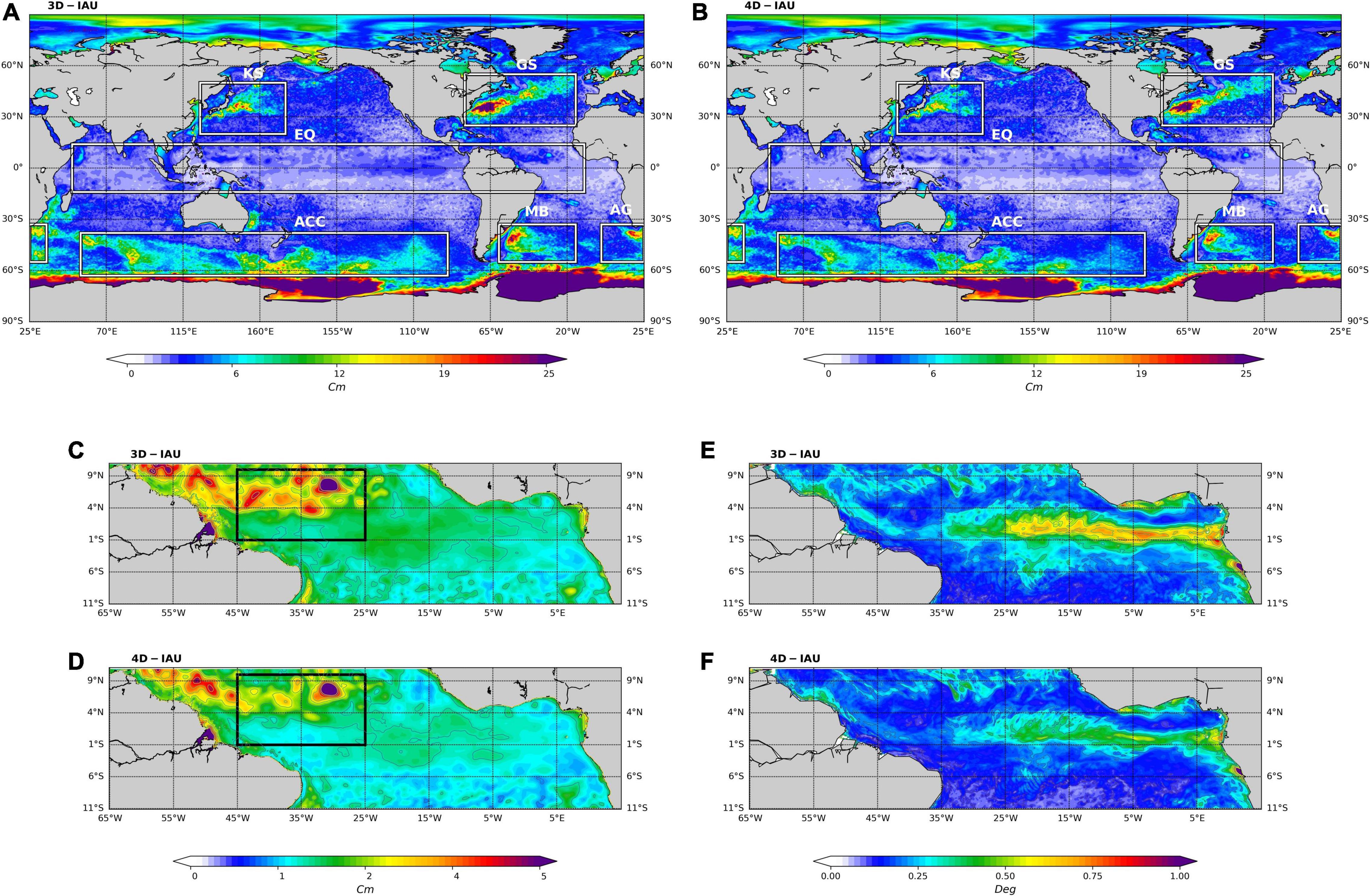
Figure 12. Root Mean Square of the SSH Error; 3D-IAU in the panel (A) and 4D-IAU in the panel (B) Gulf Stream (GS), Brazil-Malvinas confluence (MB), Kuroshio (KS) and Agulhas (AG) retroflexion, the Antarctic Circumpolar Current (ACC), and the equatorial band (EQ). Root Mean Squared of the SSH error (C,D) and SST error (E,F). (C–E) for the 3D-IAU and D-F for the 4D-IAU.

Looking at the low latitudes, the spatial RMSE for SSH and SST in the tropical Atlantic is shown in Figures 12C–F. SST variations in the cold tongue may exceed 1 °C in one week. The variability in the eastern-central region is influenced by intra-seasonal Kelvin waves coming from the west. These waves have periods of between 25 and 90 days and an estimated phase speed of 2.1 m/s (≈1,270 km/week). The northern edge of the cold tongue is influenced by Tropical Instability Waves (TIW). The 4D scheme improves the estimation of the fields almost everywhere for both variables. This illustrates the benefit of having seven increments instead of one during the cycle. The improvement in RMSE is also significant in the domain of 4°N–9°N and west of 25°W. This region has very complex dynamics with Rossby wave travelling in this region at 0.88 m/s for the first baroclinic mode (Illig et al., 2004).

To better understand which spatial and temporal scales are improved, we extended our analysis by looking at the spectral coherence between the “truth” and the assimilated experiments. For the SSH in the tropical Atlantic, the 4D experiment improves spatial coherence for all calculated wavelengths (Figure 13A). Enhancement is achieved mostly at scales greater than 100 km. Taking 0.5 coherence as a reference value, the 4D approach refines the wavelength resolution by 80km. As far as the temporal coherence is concerned (Figure 13B), the 4D approach increases coherence for periods greater than seven days. The most improved spectral band corresponds to periods between 20 and 11 days. At these period bands, the ocean dynamics are governed by local adjustment to change in winds and equatorial Kelvin waves. Surprisingly, the 3D experiment produced somewhat higher coherence for periods shorter than four days. We have two non-mutually exclusives hypotheses for this behaviour: first is that the observation network is not capable to inform about such a dynamical process and hence the information in the increments is not consistent with the true ocean state; second is that the 4D-IAU is less effective in filtering the high frequency barotropic dynamic present in the increments (Lei and Whitaker, 2016), and thus the 4D method is contaminated by high frequency noise.

FIGURE 13

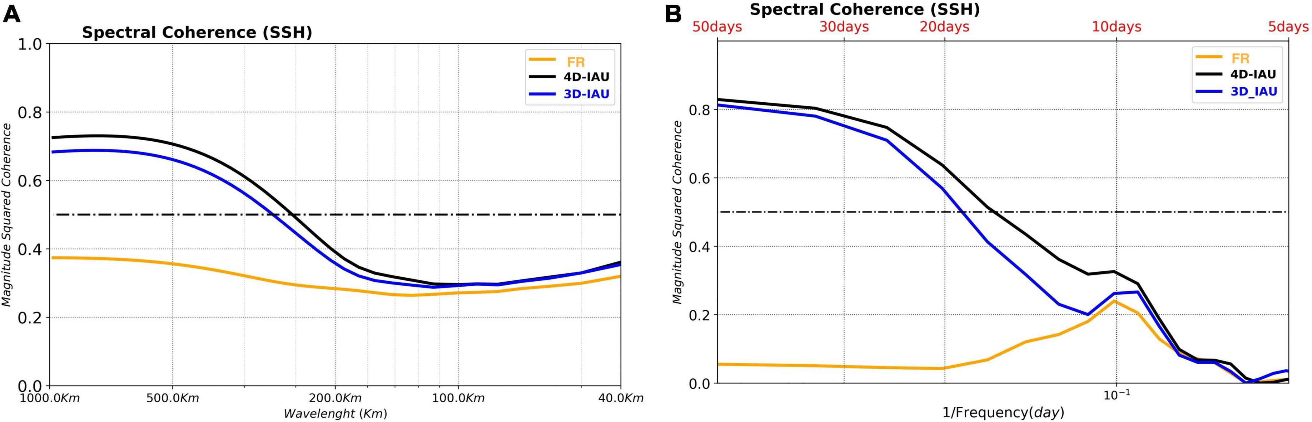
Figure 13. (A) Spatial Spectral coherence between the NR SSH and the SSH from FR (orange line), 3D-IAU (blue line), and 4D-IAU (black line). The spatial domain considered is the black box on the previous figure. (B) Time Spectral coherence on the same box.

Impact of the Improvements of the Background Error Covariances

Two identical simulations changing only the background error covariance were performed over one year (2015). SSH (J3, S3A, S3B), SST and temperature and salinity profiles were assimilated. Figure 14 shows the global SSH error standard deviation (eStd). An error reduction was observed almost everywhere, being more pronounced in western boundary currents (regions rich in mesoscale structures), Southern Ocean, and tropical regions.

FIGURE 14

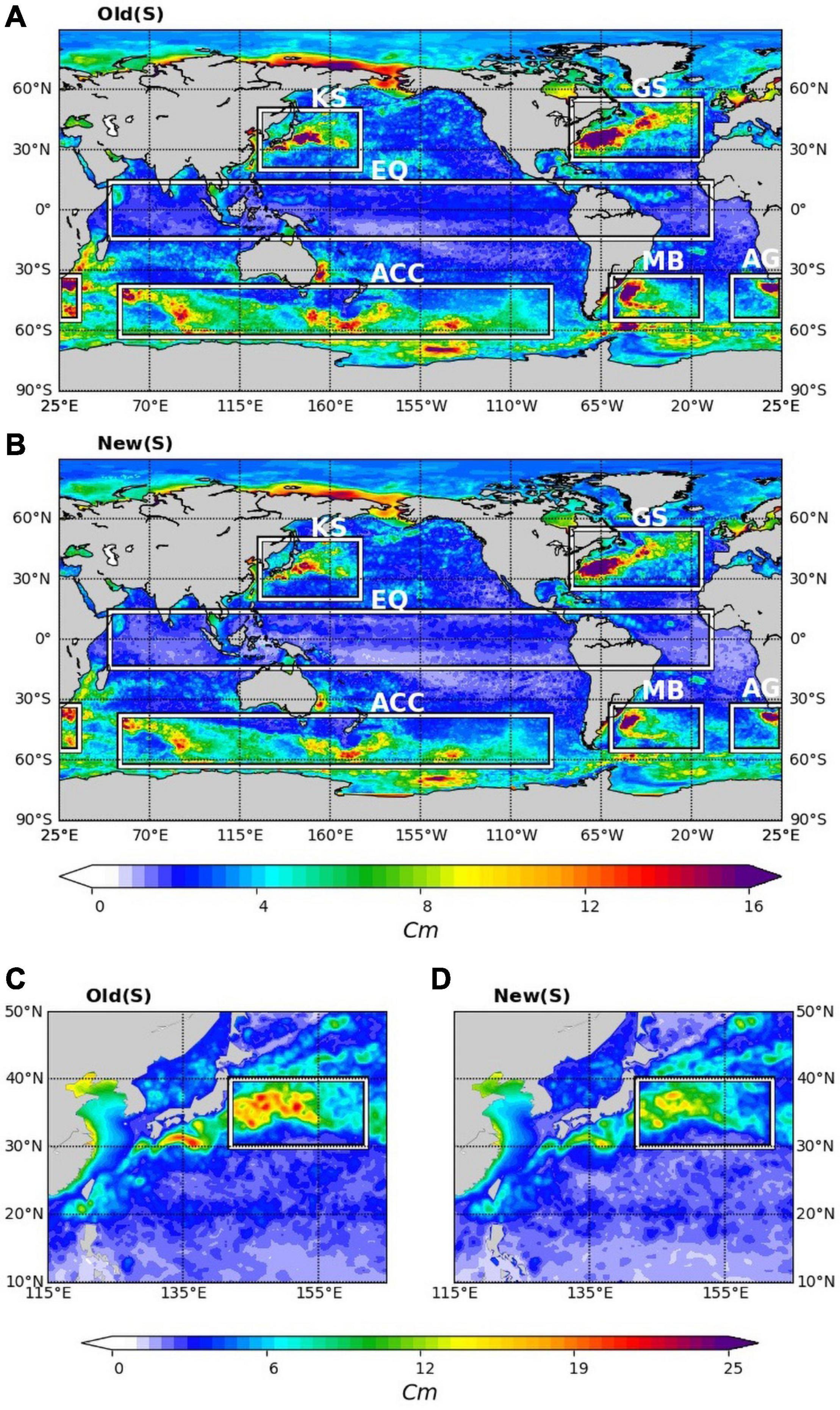
Figure 14. Standard deviation of the SSH Error (NR-Model Forecast, 2015). (A) With old background error covariance and (B) with the new background error covariance. Standard deviation of the SSH. Error on Kuroshio region (NR-Model Forecast, 2015). (C) With old background error covariance and (D) with the new background error covariance.

Next, we focussed on the highly energetic Kuroshio region. The new background error covariance improved the SSH eStd, as shown in Figure 14. To highlight this improvement, Figure 15 shows the variance preserving spectra of the SSH error calculated for the black box shown in Figure 14. This kind of spectrum is useful to see how the error variance varies as a function of wavelength. Note that the area under the curves represents the total variance of the SSH error. The SSH error is concentrated in the mesoscale band for both experiments. Using the new background error covariance reduced the SSH error for almost all wavelengths. This reduction is most pronounced in the 250–150 km range with almost a 15% error reduction. For wavelengths shorter than 50 km, both experiments had the same performance.

FIGURE 15

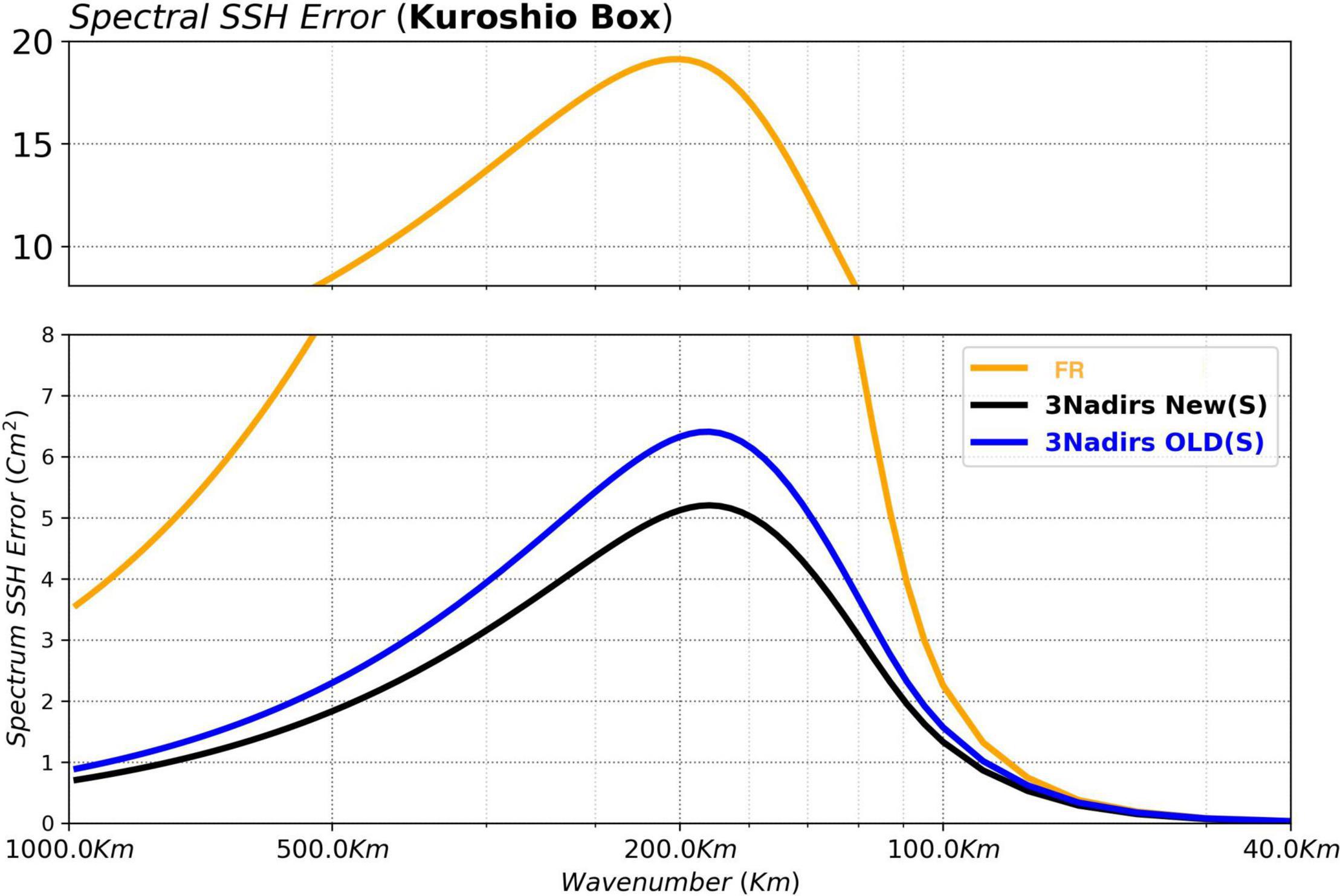
Figure 15. Power spectra of the SSH error with respect to the NR; the spectra are shown in the variance preserving form (cm²). The spatial domain considered is the black box on the previous figure.

In this section, we have shown that a careful tuning of the background error can significantly impact the assimilation system’s performance. When constructing the anomaly matrix in the same way described in section “Constructing the State Anomalies,” one should keep in mind which scales need to be constrained with the assimilation system. Of course, this is highly dependent on the model uncertainties and the structure (time and space) of the observational network.

Final Validation of OSSE Design

As outlined by Hoffman and Atlas (2016) and Halliwell et al. (2014), OSSEs must be carefully designed to produce quantitative results. In particular, this requires a high-quality NR to represent the “true” ocean, with realistic differences between the NR model and the CR model used for assimilation. It also requires the realistic extraction of simulated observations. All these aspects have been carefully analysed (see discussion in section “Nature Run and Simulated Observations”).

The entire OSSE system must also be validated to ensure that the impact of observing systems in the OSSEs is comparable to the impact of the same observation systems in the real world. This final verification of the OSSE configuration was carried out with the MOi global ocean forecasting system assimilating real observations (e.g., Copernicus Marine Service global ocean system; Lellouche et al., 2018). The objective was to verify that the innovation statistics with the pseudo-observations correspond to the real innovations of the operational system. This ensures that the OSSE design is representative of the real time system with respect to current observations.

This validation was performed by comparing our OSSE (Assimilation of data from 3 Nadir altimeters) with the G12 reanalysis which uses real data [SLA, SST, and in situ data (the CORA4.0 base)]. The calibration was done over the year 2015 that we were processing. In Supplementary Figure 1, we compare the standard deviation of SLA innovations (forecast) along the Jason tracks, in panel (A) for G12 and panel (B) for our OSSE. In the two figures we find the same patterns of maximum SLA forecast error as is often the case, with the error being larger in regions with strong currents, especially the polar fronts. On the other hand, our OSSE shows weaker errors all over the globe with an average of the order of 3.08 cm instead of 4.12 cm as per the G12. This reduction is quite clear in the tropical band and the large gyres. Supplementary Figure 1C shows the scatter diagram between the standard deviation of the SLA error between G12 and OSSE. In this figure the colour corresponds to the density of the points. For OSSE, we have a maximum of points close to 2 cm of STD error while OSE is mostly concentrated about 3 cm. Both systems have a correlation close to 82%. There are active regions where the OSSE error is larger than in reality (Gulf Stream), and others smaller (Malvinas, Kerguelen). In quieter areas, the OSSE error is smaller because the OSSE has not taken into account errors that are not directly related to SWOT, and which it is hoped to reduce in the short term. These include, for example, Mean Dynamic Topography, tidal, orbital and tropospheric correction errors.

Conclusion

The new SWOT mission introduces the need for OSSEs that fully exploit the capabilities of this new satellite, with increased observing capacity for scales down to 20 km and above 21 days. A global data assimilation system capable of assimilating SSH data from wide swath altimeters has been developed. The system is capable of assimilating a very large amount of data, as it also takes into account the assimilation of L3 SST data at high spatial and temporal resolutions. First, changes in the construction of the background error covariance matrix were described in detail Secondly, a 4D extension of the data assimilation method was presented. This will replace the old 3D FGAT system. We found a set of parameters maximising the spectral energy in the 50–250 km band. The bias correction scheme used to correct for large-scale and slowly evolving errors in the model has also been revised. The anisotropy has been reduced to a ratio of 1.5 at the equator. We have also estimated constant but different zonal and meridian radii per level with G12 over the Argo period.

A new NR simulation that serves as “truth” was presented. In NR, the smaller scales (below 100 km), which will be observed by SWOT, have a high energy level. These energy differences are mainly due to the numerical choices made for NR: absolute wind and less diffusive momentum advection scheme. NR has a realistic sea level variance and seasonal cycle. This proves the good behaviour of NR, especially with respect to the representation of vertical processes. The simulated observations were extracted from the NR simulation. The multi-sensor composites for SST, temperature and salinity profiles were extracted at the same points and at the same date as the real in-situ profiles. White noise of the order of the G12 standard deviation was added to the profiles, and 3 cm to the Nadir altimetry.

Various experiments were performed to support the design of our OSSE. The switch to the 4D SEEK improved the energetic regions (boundary and circumpolar currents). There were also clear improvements in the tropics, in the regions of tropical instability waves, equatorial upwelling and counter-currents. Basically, all areas with significant mesoscale activity and fast waves were improved, typically by 6%. In the tropical Atlantic, the switch to 4D brought an 80 km improvement in resolution. This corresponds mainly to periods of 20–11 days. The use of the new background error covariances brought a further improvement of 15% of the boundary currents. This reduction was most pronounced in the 250–150 km range. The tropics were also improved. The 4D-IAU was perhaps less effective at filtering out the high frequency dynamics present in the multiple increments and this should be improved in the future.

Finally, the design of the OSSEs was evaluated by ensuring that the differences between the assimilation system and the Nature Run are statistically consistent with the misfits between real ocean observations and the operational systems. The ocean model used in the assimilation system is an older version than the NR. There is as much difference between the new model configuration (NR) and the old one (FR) as between the G12 reanalysis and the twin free simulation. The change in the data assimilation scheme corresponds precisely to the evolution of the model: the recent configuration is almost as good as a reanalysis. There is less need to correct by assimilation for scales that are now naturally resolved with the model. The optimised bias correction parameters now match the biases of the current configurations well. There are still uncertainties in SWOT and other errors (mean dynamic topography). For this reason, the representativity error of the OSSE was kept relatively simple. The validation of our OSSE against G12 shows that our system is well calibrated and ready to be used for impact studies of future swath altimetry mission data. The results are presented in part 2 of this paper (Tchonang et al., 2021).

Data Availability Statement

The original contributions presented in the study are included in the article/Supplementary Material, further inquiries can be directed to the corresponding author.

Author Contributions

MB set up the scientific protocol of OSSEs, performed the simulations, made the first analyses of the results, and wrote the manuscript. GR, JL, EG, RB-B, and ER wrote different sections of the manuscript. P-YL, YD, and BT contributed to the analysis of the OSSEs protocol and scientific results. All authors reviewed the manuscript.

Funding

This study was funded under a CNES (French Space Agency) and Mercator Ocean partnership agreement.

Conflict of Interest

The authors declare that the research was conducted in the absence of any commercial or financial relationships that could be construed as a potential conflict of interest.

Acknowledgments

The authors would like to acknowledge the two reviewers for their valuable comments that helped improve the manuscript’s clarity.

Supplementary Material

The Supplementary Material for this article can be found online at: https://www.frontiersin.org/articles/10.3389/fmars.2021.691955/full#supplementary-material

Supplementary Figure 1 | Spatial distribution of Standard deviation of Sea Level Anomaly (SLA) error: (A) G12, (B) OSSE system, and (C) Scatter diagram between G12 and OSSE Standard deviation of SLA Error.

References

Adcroft, A., and Campin, J. M. (2004). Re-scaled height coordinates for accurate representation of free-surface flows in ocean circulation models. Ocean Model. 7, 269–284. doi: 10.1016/j.ocemod.2003.09.003

CrossRef Full Text | Google Scholar

Benkiran, M., and Greiner, E. (2008). Impact of the incremental analysis updates on a real-time system of the North Atlantic Ocean. J. Atmospher. Ocean. Technol. 25, 2055–2073. doi: 10.1175/2008jtecho537.1

CrossRef Full Text | Google Scholar

Bidlot, J.-R. (2012). Impact of Ocean Surface Currents on the ECMWF Forecasting System for Atmosphere Circulation and Ocean Waves, GlobCurrent Preliminary User Consultation Meeting. Available online at: http://globcurrent.ifremer.fr/component/k2/itemlist/category/118?Itemid=960) (accessed March 2012).

Google Scholar

Blanke, B., and Delecluse, P. (1993). Variability of the tropical Atlantic-Ocean simulated by a general-circulation model with 2 different mixed-layer physics. J. Phys. Oceanogr. 23, 1363–1388.

Google Scholar

Bloom, S. C., Takas, L. L., Da Silva, A. M., and Ledvina, D. (1996). Data assimilation using incremental analysis updates. Mon. Weather Rev. 124, 1256–1271. doi: 10.1175/1520-0493(1996)124<1256:dauiau>2.0.co;2

CrossRef Full Text | Google Scholar

Bonaduce, A., Benkiran, M., Remy, E., Le Traon, P. Y., and Garric, G. (2018). Contribution of future wide-swath altimetry missions to ocean analysis and forecasting. Ocean Sci. 14, 1405–1421. doi: 10.5194/os-14-1405-2018

CrossRef Full Text | Google Scholar

Brodeau, L., Barnier, B., Gulev, S. K., and Woods, C. (2017). Climatologically significant effects of some approximations in the bulk parameterizations of turbulent air–sea fluxes. J. Phys. Oceanogr. 47, 5–28. doi: 10.1175/jpo-d-16-0169.1

CrossRef Full Text | Google Scholar

Cabanes, C., Grouazel, A., von Schuckmann, K., Hamon, M., Turpin, V., Coatanoan, C., et al. (2013). The CORA dataset: validation and diagnostics of in-situ ocean temperature and salinity measurements. Ocean Sci. 9, 1–18. doi: 10.5194/os-9-1-2013

CrossRef Full Text | Google Scholar

Carrier, L., Matthew, J., Ngodock, H. E., Smith, S. R., Souopgui, I., and Bartels, B. (2016). Examining the potential impact of SWOT Observations in an Ocean Analysis–Forecasting System. Mon. Weather Rev. 144, 3767–3782. doi: 10.1175/MWR-D-15-0361.1

CrossRef Full Text | Google Scholar

D’Addezio, J. M., Smith, S., Jacobs, G. A., Helber, R. W., Rowley, C., Souopgui, I., et al. (2019). Quantifying wavelengths constrained by simulated SWOT observations in a submesoscale resolving ocean analysis/forecasting system. Ocean Model. 135, 40–55. doi: 10.1016/j.ocemod.2019.02.001

CrossRef Full Text | Google Scholar

Dee, D. P., Uppala, S. M., Simmons, A. J., Berrisford, P., Poli, P., and Kobayashi, S. et al. (2011). The ERA-interim reanalysis: configuration and performance of the data assimilation system. Q. J. R. Meteorol. Soc. 137, 553–597. doi: 10.1002/qj.828

CrossRef Full Text | Google Scholar

Desroziers, G., and Ivanov, S. (2001). Diagnosis and adaptive tuning of observation-error parameters in a variational assimilation. Quart. J. Roy. Meteor. Soc. 127, 1433–1452.

Google Scholar

Dibarboure, G., Pujol, M.-I., Briol, F., Le Traon, P. Y., Larnicol, G., Picot, N., et al. (2011). Jason-2 in DUACS: updated system description, first tandem results and impact on processing and products. Mar. Geodesy 34:2011.

Google Scholar

Ducet, N., Le Traon, P. Y., and Reverdin, G. (2000). Global high-resolution mapping of ocean circulation from the combination of T/P and ERS-1/2. J. Geophys. Res. 105:477.

Google Scholar

Dufau, C., Orsztynowicz, M., Dibarboure, G., Morrow, R., and Le Traon, P.-Y. (2016). Mesoscale resolution capability of altimetry: present and future. J. Geophys. Res. 121, 4910–4927. doi: 10.1002/2015JC010904

CrossRef Full Text | Google Scholar

Esteban-Fernandez, D., Fu, L.-L., Pollard, B., and Vaze, P. (2017). SWOT project mission performance and error budget JPL D-79084, Caltech. Tech. Rep. 117.

Google Scholar

Ezraty, R., Girard-Ardhuin, F., Piolle, J. F., Kaleschke, L., and Heygster, G. (2007). Arctic and Antarctic Sea Ice Concentration and Arc-Tic Sea Ice Drift Estimated from Special Sensor Microwave Data, User’s Manuel Version 2.1, CERSAT. France: IFREMER/CERSAT Brest.

Google Scholar

Farina, R., Dobricic, S., Storto, A., Masina, S., and Cuomo, S. (2015). A revised scheme to compute horizontal covariances in an oceanographic 3D-VAR assimilation system. J. Comput. Physics 284, 631–647. doi: 10.1016/j.jcp.2015.01.003

CrossRef Full Text | Google Scholar

Fu, L.-L., Alsdorf, D., Rodriguez, E., Morrow, R., Mognard, N., Lambin, J., et al. (2009). “The SWOT (surface water and ocean topography) mission: spaceborne radar interferometry for oceanographic and hydrological applications,” in Proceedings of the OCEANOBS’09 Conference (Venice-Lido).

Google Scholar

Fu, L.-L., and Ferrari, R. (2008). Observing oceanic submesoscale processes from space. Eos Trans. Am. Geophys. Union 89:488. doi: 10.1029/2008eo480003

CrossRef Full Text | Google Scholar

Gasparin, F., Greiner, E., Lellouche, J.-M., Legalloudec, O., Garric, G., Drillet, Y., et al. (2018). A large-scale view of oceanic variability from 2007 to 2015 in the global high-resolution monitoring and forecasting system at Mercator-Ocean. J. Mar. Syst. 187, 260–276. doi: 10.1016/j.jmarsys.2018.06.015

CrossRef Full Text | Google Scholar

Gaultier, L., Ubelmann, C., and Fu, L. L. (2016). The challenge of using future SWOT data for oceanic field reconstruction. J. Atmospheric Ocean. Technol. 33, 119–126. doi: 10.1175/JTECH-D-15-0160.1

CrossRef Full Text | Google Scholar

Gelb, A., Kasper, J., Nash, R. A., Price, C. F., and Sutherland, A. A. (1974). Applied Optimal Estimation. Reading, MA: M.I.T. Press.

Google Scholar

Halliwell, G. R., Srinivasan, A., Kourafalou, V., Yang, H., Willey, D., Le Hénaff, M., et al. (2014). Rigorous evaluation of a fraternal twin ocean OSSE system for the open Gulf of Mexico. J. Atmospheric Ocean. Technol. 31, 105–130. doi: 10.1175/JTECH-D-13-00011.1

CrossRef Full Text | Google Scholar

Hamon, M., Greiner, E., Le Traon, P. Y., and Remy, E. (2019). Impact of multiple altimeter data and mean dynamic topography in a global analysis and forecasting system. J. Atmospheric Ocean. Technol. 36, 1255–1266. doi: 10.1175/jtech-d-18-0236.1

CrossRef Full Text | Google Scholar

Hoffman, R. N., and Atlas, R. (2016). Future observing system simulation experiments. Bull. Am. Meteorol. Soc. 97, 1601–1616. doi: 10.1175/BAMS-D-15-00200.1

CrossRef Full Text | Google Scholar

Hunt, B. R., Kostelich, E. J., and Szunyogh, I. (2007). Efficient data assimilation for spatiotemporal chaos: a local ensemble transform Kalman filter. Physica D Nonlinear Phenomena 230, 112–126. doi: 10.1016/j.physd.2006.11.008

CrossRef Full Text | Google Scholar

Illig, S., Dewitte, B., Ayoub, N., Du Penhoat, Y., Reverdin, G., De Mey, P., et al. (2004). Interannual long equatorial waves in the tropical Atlantic from a high-resolution ocean general circulation model experiment in 1981-2000. J. Geophys. Res. Am. Geophys. Union 109:23.

Google Scholar

Kennedy, J., and Eberhart, R. (1995). “Particle swarm optimization,” in Proceedings of the ICNN’95 - International Conference on Neural Networks (Perth, WA), 1942–1948.

Google Scholar

Klein, P., Isern-Fontanet, J., Lapeyre, G., Roullet, G., Danioux, E., Chapron, B., et al. (2009). Diagnosis of vertical velocities in the upper ocean from high resolution sea surface height. Geophys. Res. Lett. 36:359. doi: 10.1029/2009GL038359

CrossRef Full Text | Google Scholar

Large, W. G., and Yeager, S. G. (2009). The global climatology of an interannually varying air–sea flux data set. Clim. Dynam. 33, 341–364. doi: 10.1007/s00382-008-0441-3

CrossRef Full Text | Google Scholar

Lellouche, J. M., Greiner, E., Bourdalle-Badie, R., Garric, G., Melet, A., Drevillon, M., et al. (2021). The copernicus global 1/12° oceanic and sea ice GLORYS12 reanalysis. Front. Mar. Sci. (accepted).

Google Scholar

Lellouche, J. M., Greiner, E., Le Galloudec, O., Garric, G., Regnier, C., Drevillon, M., et al. (2018). Recent updates to the Copernicus Marine Service global ocean monitoring and forecasting real-time 1/12° high-resolution system. Ocean Sci. 14, 1093–1126. doi: 10.5194/os-14-1093-2018

CrossRef Full Text | Google Scholar

Le Traon, P. Y. (2013). From satellite altimetry to Argo and operational oceanography: three revolutions in oceanography. Ocean Sci. 9, 901–915. doi: 10.5194/os-9-901-2013

CrossRef Full Text | Google Scholar

Le Traon, P. Y., Reppucci, A., Alvarez Fanjul, E., Aouf, L., Behrens, A., Belmonte, M., et al. (2019). From observation to information and users: the copernicus marine service perspective. Front. Mar. Sci. 6:234. doi: 10.3389/fmars.2019.00234

CrossRef Full Text | Google Scholar

Lei, L., and Whitaker, J. S. (2016). A four-dimensional incremental analysis update for the ensemble kalman filter. Month. Weather Rev. 144, 2605–2621. doi: 10.1175/MWR-D-15-0246.1

CrossRef Full Text | Google Scholar

Lellouche, J.-M., Le Galloudec, O., Drévillon, M., Régnier, C., Greiner, E., Garric, G., et al. (2013). Evaluation of global monitoring and forecasting systems at Mercator Océan. Ocean Sci. 9, 57–81. doi: 10.5194/os-9-57-2013

CrossRef Full Text | Google Scholar

Madec, G. (2008). NEMO Ocean Engine, Note du Pôle de Modélisation, Institut Pierre-Simon Laplace (IPSL), France, No. 27 ISSN, 1288–1619. (France: IPSL).

Google Scholar

Madec, G., Bourdallé-Badie, R., Bouttier, P.-A., Bricaud, C., Bruciaferri, D., Calvert, D., et al. (2017). NEMO ocean engine (Version v3.6), Notes Du Pôle De Modélisation De L’institut Pierre-simon Laplace (IPSL). Zenodo doi: 10.5281/zenodo.1472492

CrossRef Full Text | Google Scholar

Madec, G., and Imbard, M. (1996). A global ocean mesh to overcome the North Pole singularity. Clim. Dynam. 12, 381–388. doi: 10.1007/BF00211684

CrossRef Full Text | Google Scholar

Maraldi, C., Chanut, J., Levier, B., Reffray, G., Ayoub, N., De Mey, P., et al. (2013). NEMO on the shelf: assessment of the Iberia-Biscay-Ireland configuration. Ocean Sci. 9, 745–771. doi: 10.5194/os-9-745-2013

CrossRef Full Text | Google Scholar

Ott, E., Hunt, B. R., Szunyogh, I., Zimin, A. V., Kostelich, E. J., Coraza, M., et al. (2004). A local ensemble Kalman filter for atmospheric data assimilation. Tellus A 56, 415–428.

Google Scholar

Pascual, A., Faugère, Y., Larnicol, G., and Le Traon, P. Y. (2006). Improved description of the ocean mesoscale variability by combining four satellite altimeters. Geophys. Res. Lett. 33:L02611.

Google Scholar

Pham, D., Verron, J., and Roubaud, M. (1998). A Singular Evolutive Extended Kalman filter for data assimilation in oceanography. J. Mar. Syst. 16, 323–340. doi: 10.1016/s0924-7963(97)00109-7

CrossRef Full Text | Google Scholar

Pujol, M. I., Dibarboure, G., Le Traon, P.-Y., and Klein, P. (2012). Using high-resolution altimetry to observe mesoscale signals. J. Atmos. Oceanic Technol. 29, 1409–1416. doi: 10.1175/jtech-d-12-00032.1

CrossRef Full Text | Google Scholar

Purser, R. J., Wu, W. S., Parrish, D. F., and Roberts, N. M. (2003). Numerical aspects of the application of recursive filters to variational statistical analysis, Part I: spatially homogeneous and isotropic Gaussian covariances, Mon. Weather Rev. 131, 1524–1535. doi: 10.1175//1520-0493(2003)131<1524:naotao>2.0.co;2

CrossRef Full Text | Google Scholar

Qiu, B., Shuiming, C., Klein, P., Ubelmann, C., Fu, L. L., and Hideharu, S. (2016). Reconstructability of three-dimensional upper-ocean circulation from SWOT sea surface height measurements. J. Phys. Oceanogr. 46, 947–963. doi: 10.1175/JPO-D-15-0188.1

CrossRef Full Text | Google Scholar

Rodi, W. (1987). Examples of calculation methods for flow andmixing in stratified fluids. J. Geophys. Res. 92, 5305–5328. doi: 10.1029/jc092ic05p05305

CrossRef Full Text | Google Scholar

Roullet, G., and Madec, G. (2000). Salt conservation, free surface, and varying levels: a new formulation for ocean general cir- culation models. J. Geophys. Res. 105 (C10), 23927–23942. doi: 10.1029/2000jc900089

CrossRef Full Text | Google Scholar

Schouten, M. W., Matano, R. P., and Strub, T. P. (2005). A description of the seasonal cycle of the equatorial Atlantic from altimeter data. Deep Sea Res. Part I Oceanogr. Res. Pap. 52, 477–493. doi: 10.1016/j.dsr.2004.10.007

CrossRef Full Text | Google Scholar

Shchepetkin, A. F., and McWilliams, J. C. (2005). The regional oceanic modeling system (ROMS): a split-explicit, free-surface, topography-following-coordinate ocean model. Ocean Modell. 9, 347–404. doi: 10.1016/j.ocemod.2004.08.002

CrossRef Full Text | Google Scholar

Shchepetkin, A. F., and McWilliams, J. C. (2008). Handbook of Numerical Analysis: Computational Methods for the Ocean and the Atmosphere, Vol. 14. Amsterdam: Elsevier Science, 121–183.

Google Scholar

Souopgui, I., D’Addezio, J. M., Bowley, C., Smith, S., Jacobs, G. A., Helber, R. W., et al. (2020). Multi-scale assimilation of simulated SWOT observations. Ocean Model. 154:101683. doi: 10.1016/j.ocemod.2020.101683

CrossRef Full Text | Google Scholar

Tchonang, B. C., Benkiran, M., Le Traon, Y. P., Van Gennip, S. J., Lellouche, J. M., and Ruggiero, G. (2021). Assessing the impact of the assimilation of SWOT observations in a global high-resolution analysis and forecasting system. Part 2: results. Front. Mar. Sci. (Under revision).

Google Scholar

Tranchant, B., Remy, E., Greiner, E., and Legalloudec, O. (2019). Data assimilation of Soil Moisture and Ocean Salinity (SMOS) observations into the Mercator Ocean operational system: focus on the El Niño 2015 event. Ocean Sci. 3, 543–563.

Google Scholar

Verrier, S., Le Traon, P. Y., Rémy, E., and Lellouche, J. M. (2018). Assessing the impact of SAR altimetry for global ocean analysis and forecasting. J. Operational Oceanogr. 11, 82–86. doi: 10.1080/1755876X.2018.1505028

CrossRef Full Text | Google Scholar

Wu, W.-S., Purser, R. J., and Parrish, D. F. (1992). Three-dimensional variational analysis with spatially inhomogeneous covariances. Mon. Weather Rev. 130, 2905–2916. doi: 10.1175/1520-0493(2002)130<2905:tdvaws>2.0.co;2

CrossRef Full Text | Google Scholar