The Prospect of Global Coral Reef Bathymetry by Combining Ice, Cloud, and Land Elevation Satellite-2 Altimetry With Multispectral Satellite Imagery

Introduction

Accurate, high-resolution, continuous bathymetry is consistently emphasized as the most important variable to support coastal-zone management. Coral reefs are no exception. Collecting global-scale bathymetry using traditional technologies, namely sonar or airborne LiDAR, is logistically challenging and prohibitively costly, however. For this reason, there has been a search for over 50 years for a robust and reproducible way to retrieve bathymetry from satellite data (Ashphaq et al., 2021).

Ocean basin-scale bathymetry can be gathered by satellite altimetry (Smith and Sandwell, 1997), but high-resolution (meter-scale) data, particularly in shallow water, demands different techniques. The three main approaches to shallow-water bathymetry are ship-based acoustics, and active or passive optics. Ship-based acoustic methods are robust, accurate, and work in both deep and turbid water, but their coverage rates are low relative to optical air- or space-borne systems. Active optical systems use scanning lasers (LiDAR), except for a few emerging technologies such as NASA’s Multispectral Imaging, Detection, and Active Reflectance (MiDAR; Chirayath and Earle, 2016; Chirayath and Li, 2019) and airborne imaging spectroscopy (Asner et al., 2020). Passive-optical systems collect imagery, which can then be processed using a variety of techniques to derive bathymetry. Of these three technologies, passive optical systems are, as of today, the only ones which have been deployed on spacecraft and are therefore the practical choice for continuous, regional, or global-scale bathymetry measurements over coral reefs.

Many methods have been developed to derive bathymetry using passive optical systems. The techniques differ in the details, but, generally speaking, the majority of published techniques can be divided into either physically based or empirical approaches (Purkis, 2018; Kutser et al., 2020). Physical approaches use numerical models of the air-sea-seabed system. Empirical models, by contrast, are fundamentally regression-based. Empirical models are simpler to implement and more robust to noisy data than physical based approaches, but they also require extensive in situ water-depth data to tune the regression to local conditions and are therefore harder to use in a general way, say for regional or global mapping projects, than the physical approaches. Other valid, but less frequently used approaches to processing optical imagery include inferring bathymetry based on wave patterns mapped with optical or radar images (so called “wave kinematic” approaches; Abileah, 2013), stereo photogrammetry, and Fluid Lensing (Chirayath, 2016). Together, the full suite of approaches defines the domain of satellite-derived bathymetry (SDB; Goodrich and Smith, 2020).

All SDB methods would benefit if it were easier, and/or just less costly, to acquire independent bathymetric control points for training and/or validation as part of the SDB process. Empirical approaches to derive bathymetry from optical imagery could be applied more broadly, either alone or as hybrid techniques via combination with physical approaches. Physical, wave kinematic, or photogrammetric techniques would each benefit from better validation if copious directly measured bathymetry were available. Traditionally, bathymetric control points for SDB would most likely be acquired in situ with single beam echo sounders (SBES). The Advanced Topographic Laser Altimeter System (ATLAS) sensor aboard NASA’s Ice, Cloud, and Land Elevation Satellite-2 (ICESat-2) has the potential to provide global, georeferenced, high-density elevation measurements appropriate for all of these uses and could, therefore, serve as a source of remotely sensed bathymetric control points. ATLAS uses 532 nm lasers to acquire six simultaneous ground tracks with overlapping samples taken at 0.7 m spacing and a ∼17 m diameter footprint (Martino et al., 2019).

The ICESat-2 science objectives are to quantify ice-sheet elevation, sea-ice thickness, and terrestrial vegetation canopy height (Neumann et al., 2019). Even though bathymetry is not an official mission product, ATLAS’ green lasers have the potential to penetrate water and were predicted to be able to return depth measurements, based on simulations conducted prior to the launch of the spacecraft (Forfinski-Sarkozi and Parrish, 2016, 2019; Forfinski-Sarkozi and Parrish, 2019; Li et al., 2019). This capability was subsequently verified soon after launch (Parrish et al., 2019) and is the motivation for this paper. ICESat-2/ATLAS data are already being integrated into SDB workflows (Albright and Glennie, 2020; Ma et al., 2020; Babbel et al., 2021; Thomas et al., 2021), but a careful understanding of the accuracy of this data source is key to realizing that objective.

Quantifying the accuracy of ICESat-2/ATLAS bathymetry is a crucial step in building confidence in SDB products which incorporate ICESat-2 data. This study complements and builds forward from the handful of previous efforts to assess ICESat-2 bathymetry in several ways (Table 1). Except for Thomas et al. (2021), earlier efforts used data from only one site in each study, whereas this study incorporated data from nine different sites displaying a broad range in water quality, benthic character, and bathymetric complexity. Again, except for Thomas et al. (2021), other efforts compared ICESat-2 against airborne LiDAR data, but here we compare against single-beam sonar. Finally, other quantitative assessments of accuracy were reported as only an overall bias and root mean squared error (RMSE), but here we investigate depth-dependent effects as well as the effects of seabed factors, such as bottom type and roughness, on accuracy.

TABLE 1

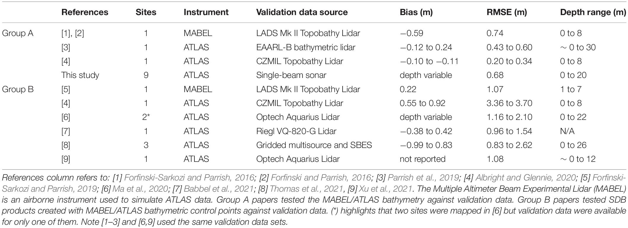
Table 1. Previous efforts to validate ICESat-2-bathymetry in comparison to this study.

Materials and Methods

Study Area and Field Data

Field data for this study were collected during the Khaled bin Sultan Living Oceans Foundation’s (KSLOF) Global Reef Expedition (GRE), which consisted of a global transect of shallow-water coral reef sites conducted between 2006 and 2015. As part of this effort, over 65,000 km² of bathymetric and benthic habitat maps were produced from WorldView-2 satellite imagery fused with copious in situ data (Purkis et al., 2019). The key GRE in situ data used for this project were soundings collected by a research-grade single-beam echo sounder at each of the survey sites.

The GRE mission visited > 1,000 sites in 15 separate countries. Sites typically corresponded to individual atolls (e.g., Mangareva or Raivavae, French Polynesia) or isolated flat-topped carbonate platforms (e.g., Cay Sal, Bahamas or Ha’apai, Tonga). For the purposes of this paper, we considered a “site” to be an area that was mapped during the GRE as a single contiguous map product (Figure 1). At each site, WorldView-2 and/or -3 satellite imagery was mosaicked and processed with object-based image analysis software to create a benthic habitat map and with a band-ratio approach to create continuous bathymetric maps (Purkis et al., 2019). Also, at each site, a small skiff outfitted with a HydroBox HD hydrographic echo sounder collected bathymetric transects. Over 30 million sonar soundings were collected in total under the auspices of the GRE. Soundings were corrected for the offset of the transducer below the waterline and ultimately used to calibrate and validate the bathymetric maps which were optically derived from satellite imagery using the multi-regression approach developed by Kerr and Purkis (2018). Nine GRE survey sites were chosen for this study (Figure 1). As described below, for each of these sites, the GRE echosounder data were quantitatively compared with the ICESat-2 LiDAR bathymetry. The GRE habitat and satellite-derived bathymetric maps were used to stratify this comparison in order to examine if there were systematic biases by habitat or seabed roughness.

FIGURE 1

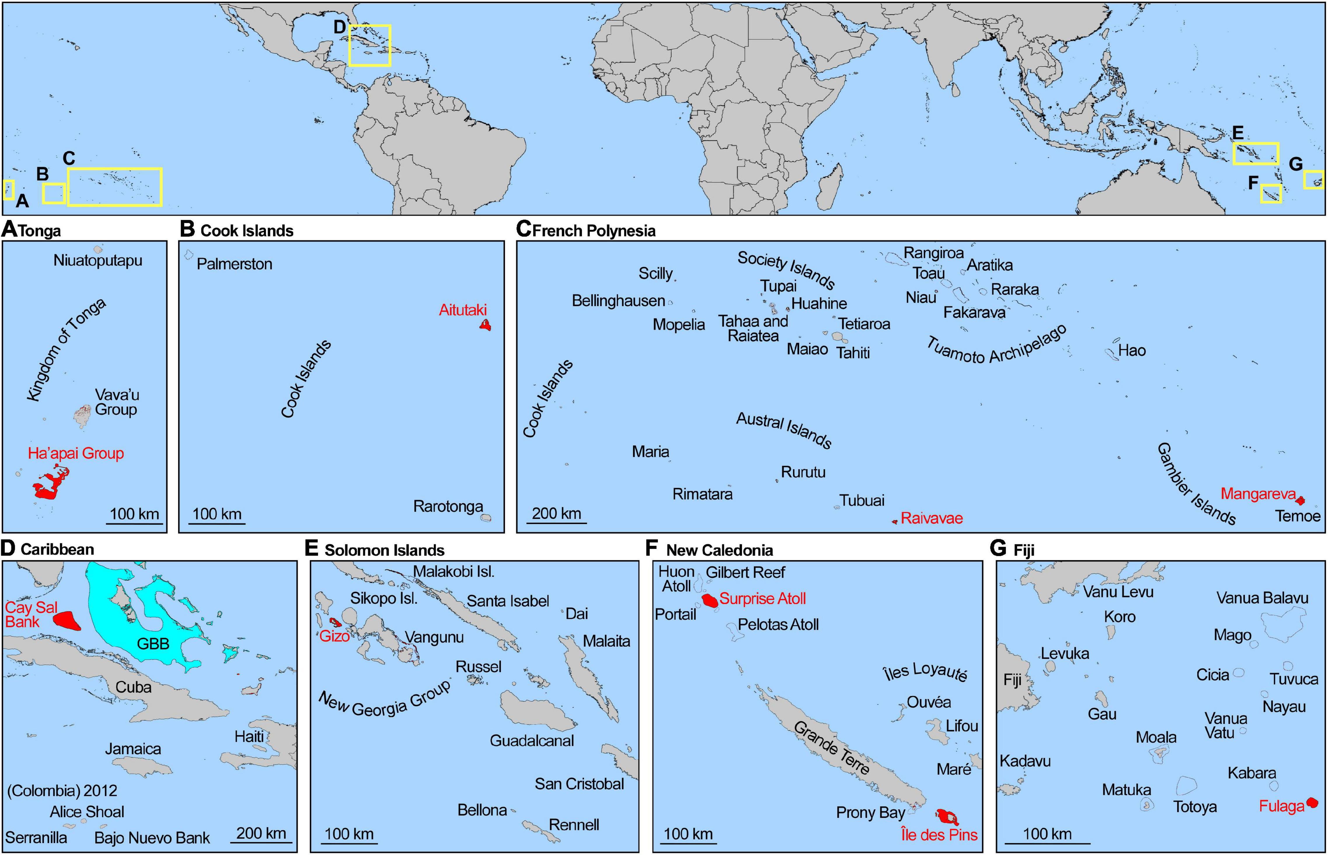
Figure 1. Locations of study sites are highlighted in panels (A–G), in red, as well as nearby geographic features. Extents of each panel (A–G) are shown in the top panel. The GBB in panel D stands for “Great Bahama Bank.” North is top in all maps; scales as noted.

Ice, Cloud, and Land Elevation Satellite-2 Water Depths

First, ICESat-2 ATL03 geolocated photon data was acquired from the NASA National Snow and Ice Data Center Distributed Active Archive Center (NSIDC DAAC) application programming interface (API). For each GRE site, a polygonal area of interest was submitted to the API via TCarta’s Space Based Laser Bathymetry Extraction Tool software, which returned a set of Hierarchical Data Format Files (HDF5) containing subset data for each coincident ATL03 data granule.

Next, a pre-processing routine was applied to each ATL03 dataset, in which all photon measurements were converted from ellipsoidal heights to orthometric heights using the EGM2008 geoid model and referenced to all necessary hierarchical metadata including sensor geometry and incident angle.

To extract bathymetry measurements, each of the six individual laser transects within the ATL03 datasets were visualized in the Space Based Laser Bathymetry Extraction Tool graphical user interface (GUI) and reviewed for evident seafloor returns (Figure 2). Where viable bathymetry was found, a clustering algorithm was applied to delineate sea surface and seafloor photons. A Density-Based Spatial Clustering of Applications with Noise (DBSCAN) algorithm was used to aggregate photon returns based on spatial density, whereby photon clusters are constrained using maximum neighbor radius and minimum cluster sample count parameters.

FIGURE 2

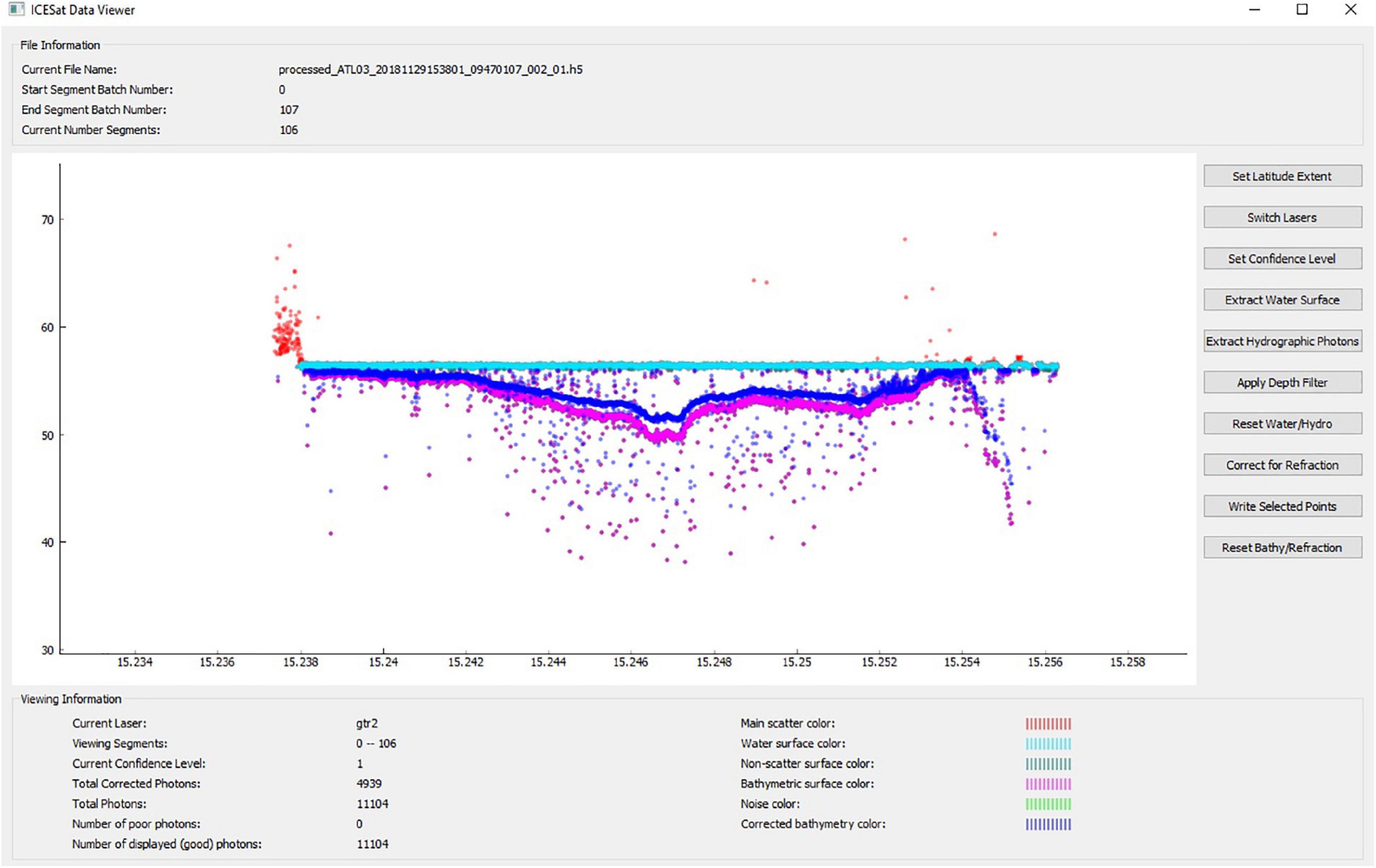
Figure 2. SBL Tool GUI with delineated sea surface and refracted seafloor photon returns.

Within the ATL03 photon point cloud, the sea surface is commonly resolved as tightly clustered photon returns with a linear distribution across the entire transect of ATL03 data. Therefore, the DBSCAN algorithm was passed a small radius constraint, 0.05–0.1, depending on the specific dataset, and a high minimum sample size, 500–1,000, again dependent on the specific dataset. Once suitably delineated, the median sea surface photon orthometric heights were stored for use in the refraction calculation and relative water depth calculation, and excluded from the dataset of photons submitted to seafloor delineation.

Seabed returns were also delineated with the DBSCAN clustering algorithm. Although not as densely defined as the sea surface, ATL03 seabed photon returns are relatively dense compared to erroneous water column artifacts. With these considerations in mind, radius constraints between 0.25 and 1.0 were used, with minimum sample counts between 2 and 10. A smaller radius and larger sample count will only cluster clearly defined seafloor photons but may not include more sparse seafloor photons. A larger radius and smaller sample count results in more clustered seafloor photons, but also includes additional erroneous returns which must be manually removed during point cloud editing, following depth derivation. Once the seafloor photons were sufficiently delineated, the seafloor photons were submitted to a refraction algorithm.

The refraction algorithm was used to calculate the true latitude, longitude and orthometric height, correcting for the effects of light refraction through water, referencing the methodology found in Parrish et al. (2019). This process employs the median sea surface photon-orthometric height value, the specific dataset sensor collection geometry, a refractive index of 1.33 × 10^–4 (Quan and Fry, 1995), and each seabed photon’s apparent latitude, longitude and orthometric height to calculate the true, refracted position of each seabed photon. Following refraction correction, a relative water column depth for each refraction-corrected seafloor photon was determined by calculating the difference between the photon’s refracted orthometric height and the local sea surface median orthometric height. To correct for the effect of ocean tides, all relative water column depths were corrected to lowest astronomical tide (LAT) datum using temporally specific tide height predictions derived from ADMIRALTY TotalTide software. Finally, all data were visualized in a three-dimensional point cloud environment and any residual outlier depth measurements were removed.

Analyses

The first step was to associate ICESat-2 and in situ sounder samples. For each ICESat-2 point, the single-beam echosounder records were searched to find all echoes within 8.5 m, which is the nominal radius of the ICESat-2 footprint. An ICESat-2 sample and the sonar echoes coincident within its footprint were considered a matching pair, or “matchup.” Two metrics were computed for each matchup: the mean depth of the sounder points and the lag, defined as the mean distance to all the matched sounder points.

The second step of analysis was to calculate the correlation between sounder and ICESat-2 matchups. This was performed with the Matlab (version R2020b) “fitlm” and “ttest” functions, returning the slope, intercept, root mean squared error, and R² coefficient for a least squares fit, as well as mean, standard deviation and 95% confidence interval for the distribution of differences between the ICESat-2 and the sounder water depths. Using ordinary least squares regression (OLS) to compare sounder and ICESat-2 matchups had the potential to give misleading correlations if the data were noisy or contained outliers. Moreover, OLS tends to decrease the slope of the fitted line as the correlation decreases (i.e., for lower R² values), which was undesirable since we wanted to see if the sounder and ICESat-2 matchups fell on a 1:1 line. Thus, robust least squares (RLS) and principal components based (PCA) regressions were also computed using the Matlab “fitlm” and “pca” functions, respectively. Regressions were computed using all three methods for each site individually as well as for the entire dataset as a whole, by pooling data from all sites.

The third step of analysis was to consider possible factors affecting differences between ICESat-2 and sonar-depth retrievals. Using the maps described above (Section “Study Area and Field Data”), matchups were grouped by the habitat where they were sampled (Table 2), as extracted from the GRE benthic habitat maps and associated ground control. Next, the depth variability around each ICESat-2 sample was computed as the standard deviation of a 14 × 14 m window around each point. Univariate plots illustrated the effects of depth, habitat, and depth variability on the difference between ICESat-2 and sonar-depth retrievals. We used a generalized estimating equations (GEE) model to quantitatively assess the combined effects of these factors. The GEE model estimated the mean association between the error, computed as ICESat-2 minus sounder depth differences, and several attributes: the depth of the measurement itself, the mean distance between the two measurements, the roughness of the surrounding seabed, and a binary variable indicating whether the two measurements occurred in the same GRE habitat class. A GEE model was utilized due to suspected correlation within same geographic area and the correlation structure was chosen via minimized quasi-information criteria (QIC; Pan, 2001). P-values less than 0.05 were considered statistically significant and all analyses were performed in R version 4.04 and the gee package version 4.13-20.

TABLE 2

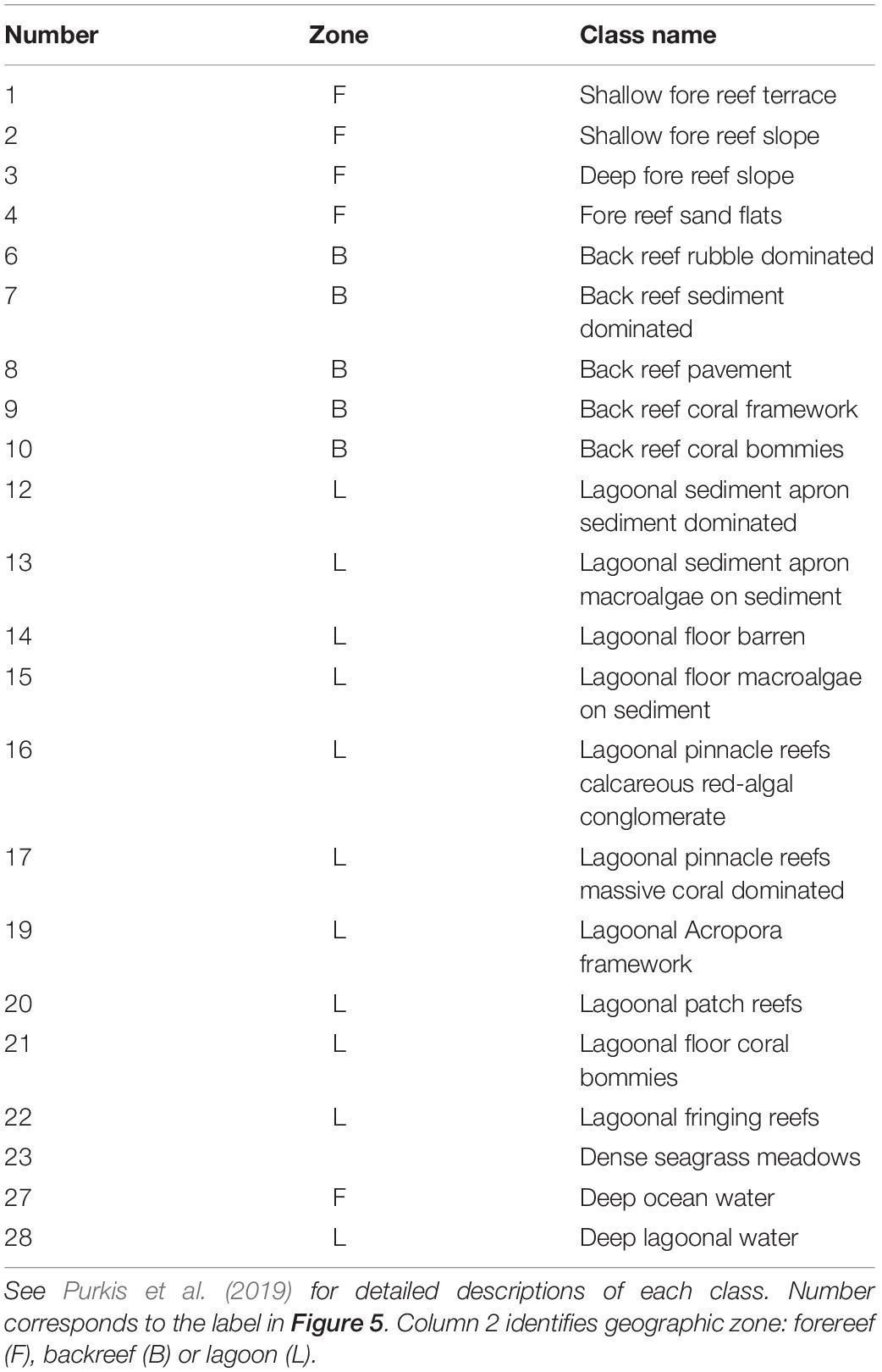
Table 2. Benthic habitat classes.

Finally, we accommodated discrepancy in reported values for the nominal ATLAS beam footprint diameter. Design specifications were for <17.5 or 17.4 m (Markus et al., 2017; Neumann et al., 2019). Early post-launch reports were <17 m (Martino et al., 2019) or 17 m (Parrish et al., 2019; Albright and Glennie, 2020). A recent paper and the current ICESat-2 technical specifications web page cite 13 m (Thomas et al., 2021). Another recent paper uses 11 m (Babbel et al., 2021). Given the variance in these values we conducted the entire analysis described above using both 8.5 m and 6.5 m radii for matching echoes to ICESat-2 data.

Results

Over six million echo soundings and almost 8,000 ICESat-2 depth retrievals were available at the nine sites used for this study. Of these, 1,573 ICESat-2 records matched up with at least one sonar sounding within its 17 m diameter footprint (Table 3). Overall, the median number of soundings per matchup was 59. This was a skewed distribution with 22 ICESat-2 records having only 1 sonar sounding in their footprints and 1 ICESat-2 record having 819 sonar soundings in its footprint.

TABLE 3

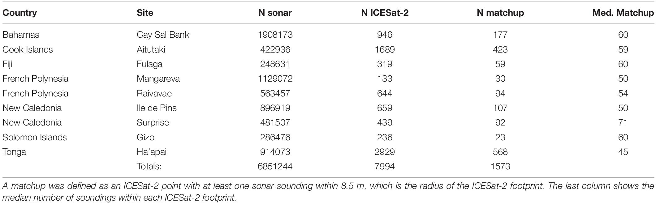
Table 3. The first 3 columns following the country and site names show the number of echo soundings, ICESat-2 depth retrievals, and matchups between the two by site.

There was a high correlation between ICESat-2 and coincident single-beam echo sounder depths when data were pooled across all sites (slope = 0.83, R² = 0.96, N = 1,573; Figure 3). Ice, Cloud, and Land Elevation Satellite-2 has dense along-track sampling, so many of the ICESat-2 measurements overlapped, therefore many sonar soundings were within 8.5 m of more than one ICESat-2 point. In other words, not all the matchups were independent samples. Unique matchups were identified as those with smallest average lag, producing a smaller dataset of non-overlapping samples. There were no significant differences between the correlations using all matchups as compared to the “unique” matchups (slope = 0.83, R² = 0.96, N = 397; Figure 3). Overall, the sounder recorded slightly deeper depths than ICESat-2. Mean ICESat-2 minus sonar depth (and 95% confidence interval) was −0.36 m (−0.41 to −0.31 m) for the full set of matchups and −0.23 m (−0.33 to −0.12 m) for the unique set. Linear regression for both the full and unique sets of matchups revealed a depth-dependent bias (slope < 1). Sonar depths were deeper than ICESat-2 depths in shallow water and vice-versa in deeper water.

FIGURE 3

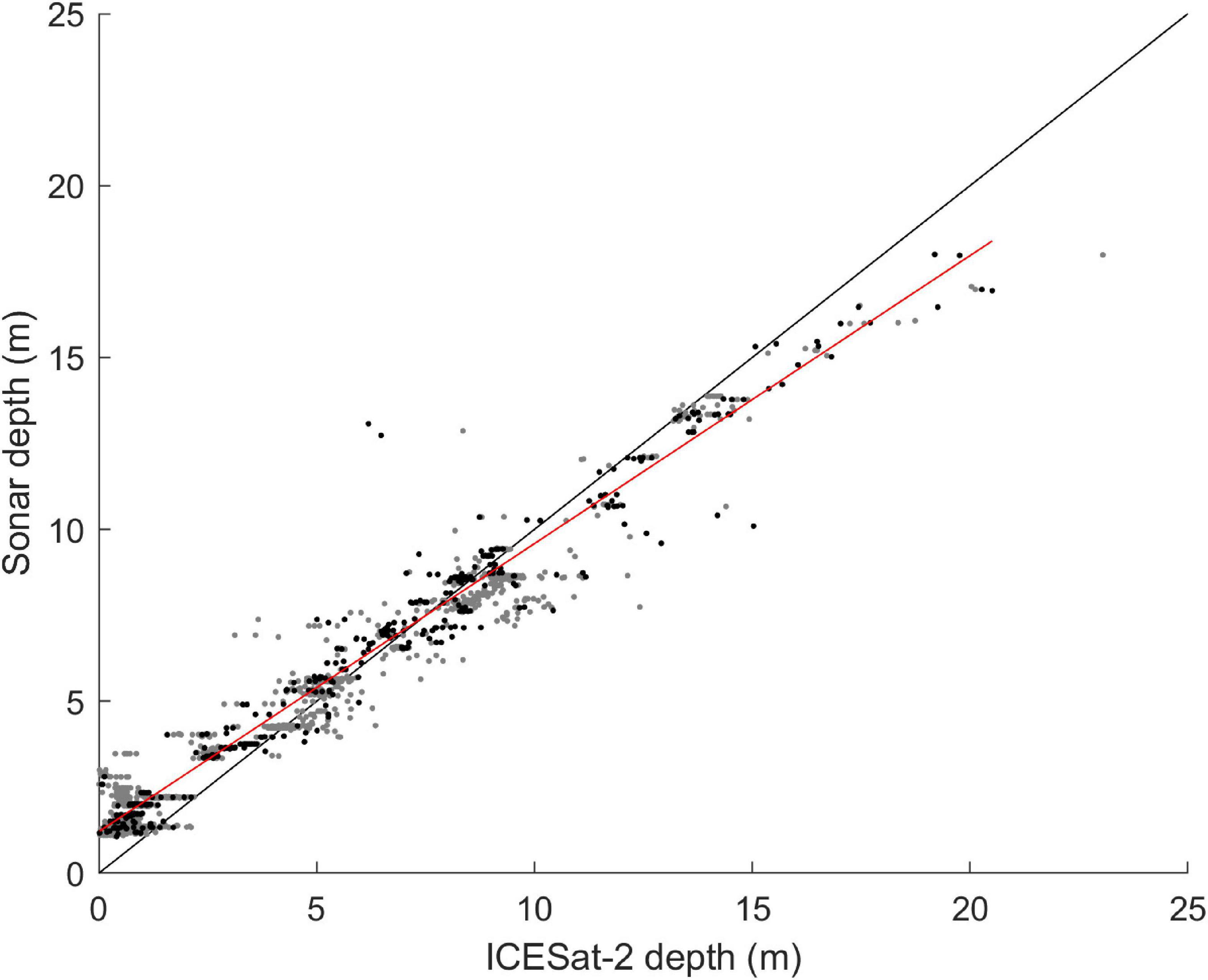
Figure 3. Correlation between depths recorded by ICESat-2 and single beam sonar. Each sonar point on this plot is an average of all echoes located within 8.5 m of the corresponding ICESat-2 return (N = 1573 matchups). Points shown in black contain unique combinations of sonar points in their average (N = 397). Points in grey contain echoes that are also averaged in other matchups. Linear fit shown to the unique data only (black points; R² = 0.96 and slope = 0.84) but the fit to all the data has same R² and slope = 0.83.

High correlations between ICESat-2 and coincident single-beam echo sounder depths were also found when data were analyzed at each site separately (Figure 4 and Table 4). All the sites had R² ≥ 0.92 for ordinary least squares fits except Gizo (Solomon Islands) and Surprise (New Caledonia). Robust least squares regression changed the R² value by more than 0.02 at only Gizo, Surprise, and Mangareva (French Polynesia; Table 4). The slopes of the fits, as determined by OLS, RLS, and PCA were very similar for all sites except Mangareva and Surprise (Table 4). Mangareva and Surprise each had 2-3 outliers, which were identified and removed by RLS fitting. Fulaga (Fiji) and Surprise were the only sites with slopes greater than 1:1, although the slope for Surprise dropped to 0.95 when accounting for the outliers with RLS regression.

FIGURE 4

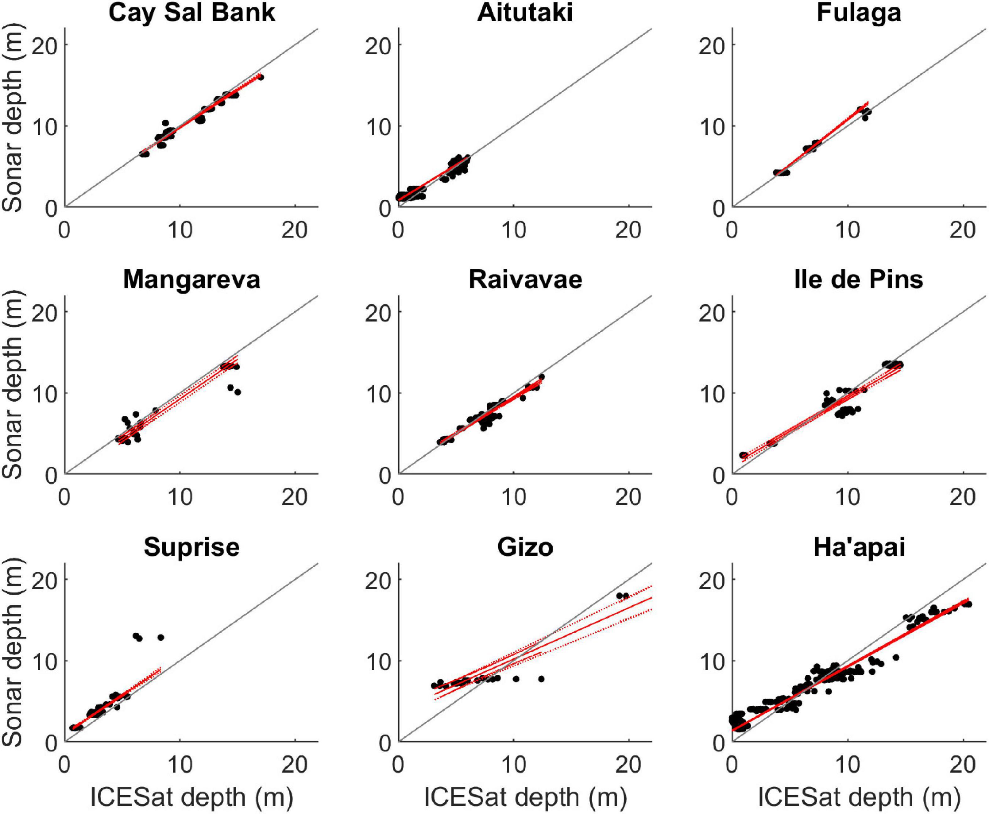
Figure 4. Correlation between depths recorded by ICESat-2 and single-beam sonar at each site. Each sonar point on this plot is an average of all echoes located within 8.5 m of the corresponding ICESat-2 return. The 1:1 line and robust least squares fits are plotted as well as the confidence interval of the RLS fit; see Table 3 for summary of fits to data.

TABLE 4

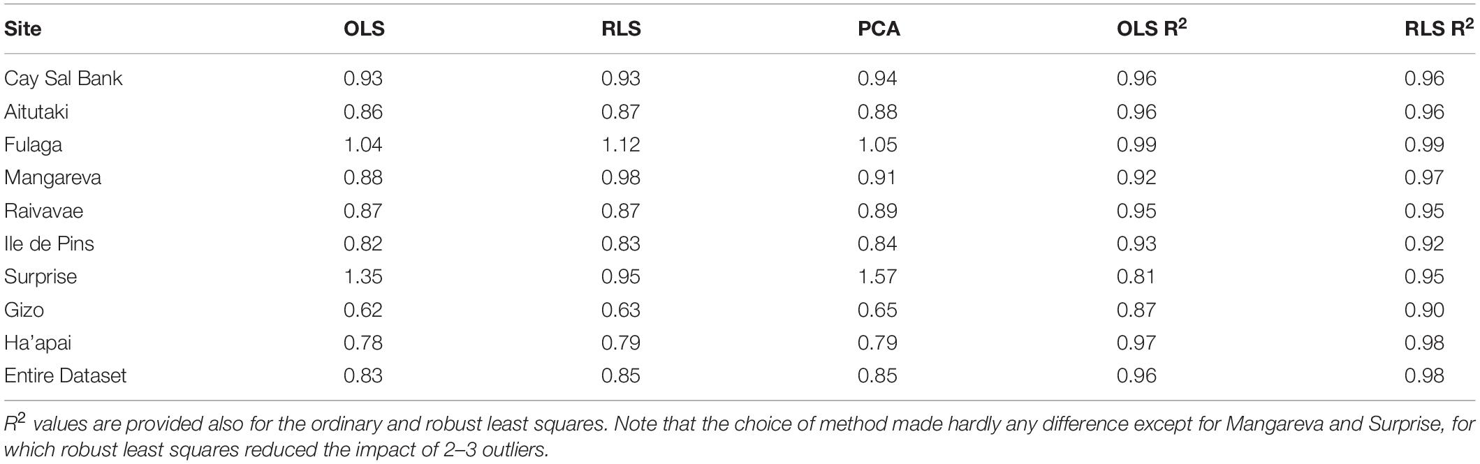
Table 4. Summary of linear fits to data. OLS, RLS, and PCA are the slopes of fits to the data using ordinary least squares, robust least squares and principal components analysis regression, respectively.

Average differences between ICESat-2 and sonar depth measurements did vary among habitat type (Figure 5). The boxes in Figure 5 define the interquartile range (range containing the middle 50% of the values), with the horizontal line in the middle of each box marking the median. Dashed lines extend ± 1.5 times the interquartile range or to the maximum/minimum values, whichever is less. Symbols (+) mark outliers, defined as values >1.5 times the interquartile range outside the middle 50% of data.

Although different habitats exhibited different average differences between ICESat-2 and sonar depths, it was difficult to find systematic differences that could be ascribed to benthic cover or seabed relief. The habitat classes with the largest absolute differences between ICESat-2 and sonar depths did not systematically vary in substrate, roughness, nor geographic zone (Figures 5, 6 and Table 2). The class with the most positive ICESat-2 – sonar difference was a low-relief sediment class (#12, “Lagoonal sediment apron”). Classes with the third through fifth most positive ICESat-2 – sonar difference, on the other hand, were high relief reef (classes 10, 17, and 20). The class with the second most positive ICESat-2 – sonar difference (#28) was “deep lagoonal water” which means analysts making the habitat maps could not identify the seabed type due to the water depth, so the actual habitat in class 28 could have been several different things. Of the four classes with most negative ICESat-2 – sonar difference, two were in the forereef (classes 3, 4), two in the back reef (classes 9, 6); two were low relief (4, 6), and two were high relief (9, 3). In short, although there were average differences among the matchups when grouped by habitat, there was no obvious pattern to which seabed classes produced positive vs. negative ICESat-2 – sonar difference.

FIGURE 5

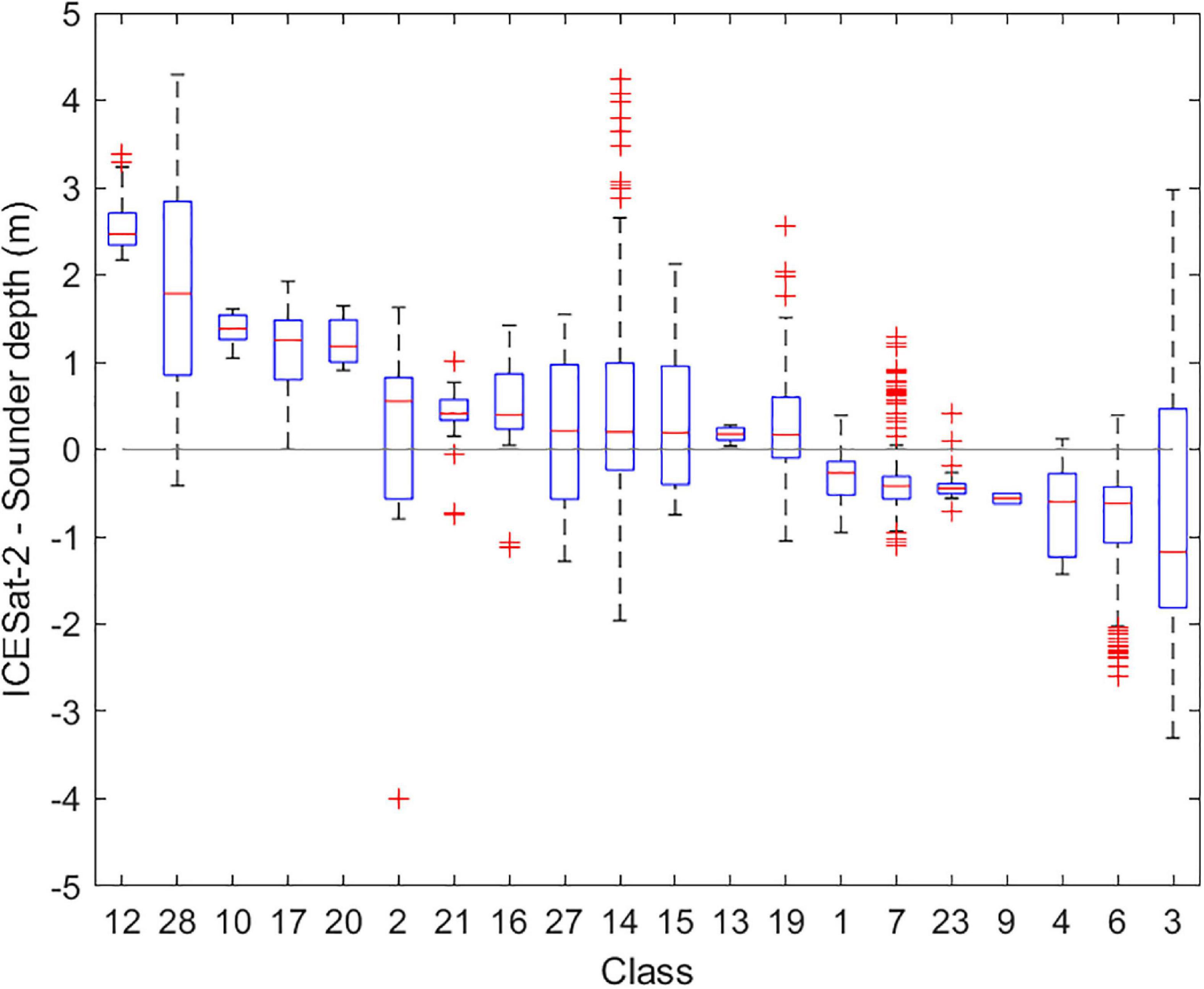
Figure 5. The difference between depths recorded by ICESat-2 and single beam sonar categorized by seabed habitat class. Boxplots show the median, interquartile range, overall extent of data and outliers for each class; see text for details. Classes are sorted in this figure in order of decreasing median ICESat-2 – sonar depth difference. Note lack of obvious patterns in classes with large positive or negative median values (Table 2 defines the class names).

FIGURE 6

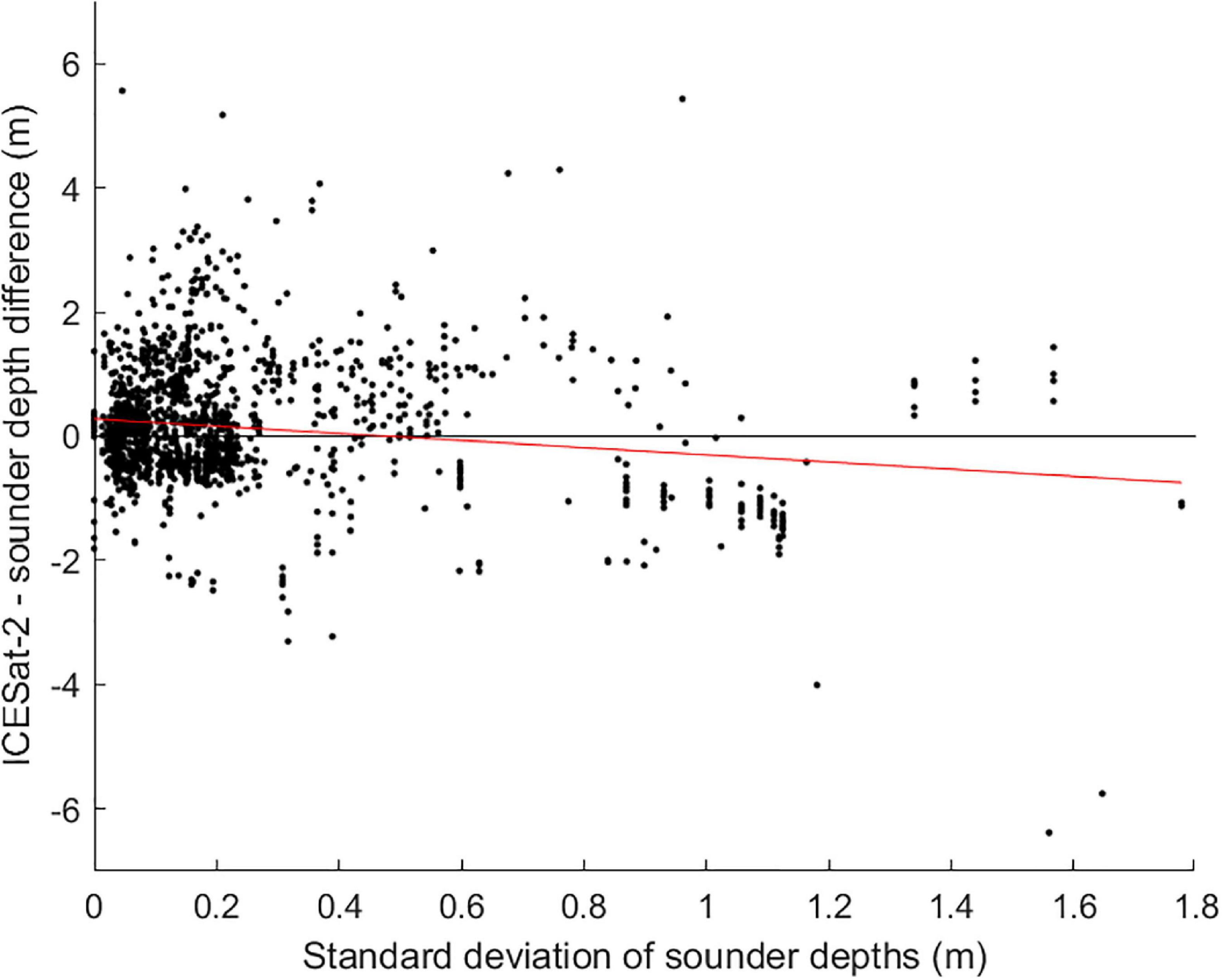
Figure 6. The difference between depths recorded by ICESat-2 and single beam sonar plotted against the standard deviation of sonar depths in the neighborhood around each point. Linear fit to these data plotted as a red line. Note, however, negative correspondence between the ICESat-2 – sonar difference and seabed roughness was not found to be statistically significant in the multivariate GEE analysis (Table 5).

TABLE 5

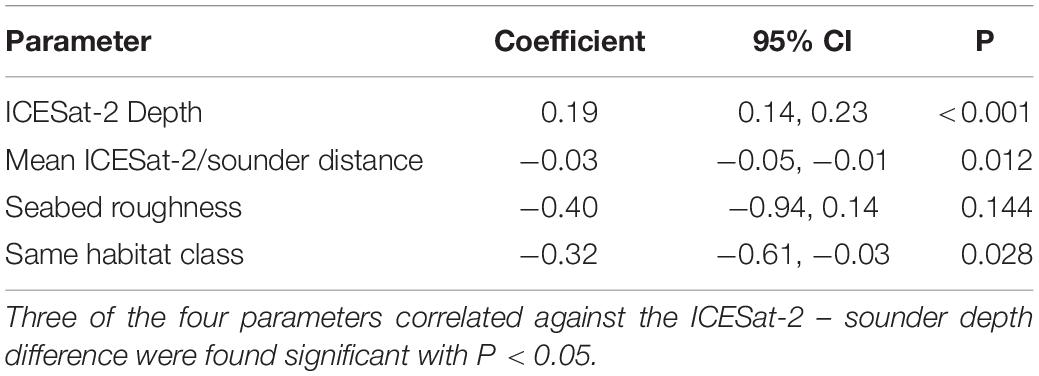
Table 5. Generalized estimating equations (GEE) model results.

The multivariate GEE model assessed combined effects of depth, geolocation offset, seabed roughness, and habitat edges on the difference between ICESat-2 and sounder measurements. This model complemented the univariate results (Figures 5, 6) by controlling for multiple factors simultaneously. Multiple correlation structure settings were tested when developing the GEE model. The exchangeable correlation specification was chosen for the analysis because, of those that were computationally feasible, it resulted in the lowest QIC. Three of the four variables included in the model were found statistically significantly correlated with the ICESat-2 – sonar depth difference (Table 5). On average, the ICESat-2 – sonar depth difference increased by 0.19 m (95% CI: 0.14, 0.23, p-value < 0.001) for each 1 m increase of depth, decreased by −0.03 m (95% CI: −0.05, −0.01, p-value: 0.012) for every 1 m increase in average distance between the ICESat-2 center and the matching sonar soundings, and decreased by −0.32 m (95% CI: −0.61, −0.03, p-value 0.028) if the two measurements were in different habitat classes. The ICESat-2 – sonar difference was negatively correlated with seabed roughness, but this was not found statistically significant by the GEE model (Figure 6 and Table 5).

Virtually no differences were obvious for any of these tests regardless of whether the matchups were performed with an 8.5 m or 6.5 m ICESat-2 footprint radius. The linear regression using all matchups within 6.5 m yielded a slope of 0.85 (R² = 0.97, N = 1,221) and using only the “unique” matchups within 6.5 m also gave a slope of 0.85 (R² = 0.96, N = 398). The plots of differences by roughness and habitat were also essentially identical to the values using 8.5 m radius. In short, the choice of ICESat-2 footprint size made no meaningful difference to the results.

Discussion

There was a high correlation between ICESat-2 and coincident single-beam echo sounder depths (R² = 0.96), and a low overall mean difference (−0.36 m for the full dataset). There was also a depth-dependent bias, however, manifested by a slope less than 1 overall, and at all sites except Fulaga, individually. Sonar depths were deeper than ICESat-2 depths in shallow water and vice-versa in deeper water (Figures 3, 4). What factors might be the cause of this depth-dependent bias between the datasets? How do these results fit in the context of others that have used ICESat-2 for SDB?

One source of bias might be any factor affecting detection of the seabed in the raw data. The raw signals recorded by both ICESat-2 and single-beam sonars are both fundamentally an intensity signal as a function of time. These waveforms must be analyzed to detect the location of the seabed, a process colloquially known as “bottom picking.” In the case of LiDAR instruments, such as ICESat-2, the sea surface must also be detected, but the process is conceptually the same. Bottom-picking algorithms are automated, by the necessity to process millions of signals efficiently, and, although generally robust, they can be fallible. Seabed roughness, and backscattering elements in the water column are factors that could affect bottom (or sea surface) picking algorithms for both optical (LiDAR) and acoustic signals. Seabed reflectance in the sense of color (for optical signals) and impedance (for acoustic signals) is another factor that can affect bottom-picking algorithms.

We did not have independent geophysical data such as bottom impedance or optical albedo at the sites of the matchups, however, we did have habitat data, which can be considered as a proxy for both seabed albedo and impedance (Gleason et al., 2009, 2011). Habitats, almost by definition, vary in seabed reflectivity (color and optical impedance), roughness, and often affect the color of the overlying seawater (e.g., clear forereef vs. optically shallower lagoon). Habitats, therefore, integrate these factors into coherent units. Systematic differences between smooth, flat habitats (sand, for instance, or pavement) and rugose or sloping ones (forereef perhaps) would support the hypothesis that bottom pick was a source of bias. Habitats did vary in their median ICESat-2 – sounder depth differences (Figure 5). Also, the GEE model detected a small edge effect, whereby matchups near a class border had ICESat-2 – sonar depth difference 0.32 m less than those sites not near a habitat edge, on average (Table 5). It makes sense that measurements taken over different habitats would have a larger absolute difference than those taken in the same habitat. The edge effect did not explain the depth-dependent bias in ICESat-2 – sonar depth difference, however, which was still 0.19 m per m depth increase even when controlling for habitat edge (Table 5). Moreover, as discussed in the results section, above, the patterns of differences as grouped by habitat did not suggest any obvious systematic effects; low- and high-relief habitats had both positive and negative median ICESat-2 – sounder depth differences, for example. This too was reflected in the GEE model, which demonstrated that the negative correlation between seabed roughness and ICESat-2 – sounder depth difference was not statistically significant (Table 5).

Depth calculation could be another source of bias. Calculating depths with echosounders requires converting time to distance by knowing the speed of sound in seawater (c). Most single-beam echo sounders, including the one used in this study, assume a constant value of c, but, in reality, c varies as a function of the temperature, pressure, and salinity of the water body. An inaccurate value of c would therefore affect the slope of sonar depths vs. ICESat-2 depths because the magnitude of error increases linearly with depth. Systematically adjusting sonar depths by an assumed error in c and recomputing the regression of adjusted sonar depths vs. ICESat-2 depths revealed that a ∼23% increase in c would result in a 1:1 slope. This is an unrealistically large error, however. Near the ocean surface, c varies by <3% over the range of salinity (34 – 36 ‰) and temperature (20 – 30°C) relevant to the study areas (Del Grosso, 1974).

To place this work in the context of other studies, it is important to appreciate the distinction between validating ICESat-2 bathymetric data itself as opposed to validating SDB products which were derived using ICESat-2 data as bathymetric control points (Table 1). The former is the subject of this paper and a direct measure of ICESat-2 data quality whereas the latter convolves ICESat-2 data quality with satellite data quality and algorithmic limitations. Of course, it is the latter that ultimately matters (how accurate is your map?), but both types of studies are necessary in order to partition the error sources in a final map.

Babbel et al. (2021), for example, used the Stumpf et al. (2003) algorithm, seeded with ICESat-2 bathymetric control points and noted that the errors between their SDB and the airborne LiDAR data that they used for validation varied among different zones of their study site. They felt that environmental conditions within their study site, such as spatially varying turbidity or seabed types were likely causing spatial variation in SDB accuracy. Indeed, it has long been recognized that dark habitat tends to come out as artificially deep and light habitats as artificially shallow when using the popular Stumpf et al. (2003) SDB bathymetry algorithm (or others based on the same premise). The question is whether these effects are wholly caused by algorithm limitations or whether the ICESat-2 bathymetry itself suffers from errors due to bottom brightness and/or water quality. The result that ICESat-2-sonar differences were not systematically biased by habitat or roughness (Table 5) is noteworthy because it suggests that the problem observed by Babbel et al. (2021) is with the SDB algorithm, not the ICESat-2 data. This means that the ICESat-2 data are unlikely to exacerbate the darkening problem of these Stumpf-type SDB algorithms.

All of the other studies that have considered the accuracy of ICESat-2 bathymetry (as opposed to SDB accuracy) compared against airborne LiDAR (Table 1). None of these reported a depth-dependent bias, which is consistent with TCarta internal unpublished data (also compared against airborne LiDAR). On the other hand, none of the other studies reported error as a function of depth so we do not really know. Generally, other studies have reported summary statistics such as RMSE and overall mean bias. Our values for both of these are in line with previous work (Table 1).

The only other study of ICESat-2 bathymetry to use SBES as a validation data source was Thomas et al. (2021). They assessed SDB seeded with ICESat-2 data rather than ICESat-2 bathymetry itself and found depth-dependent bias indicating SDB was deeper than SBES in shallow water and shallower in deeper water, which is the opposite of what we found here (they had a slope of 1.24 vs. our slope of 0.83). Interestingly, Ma et al. (2020, their Figure 11) also found depth-dependent bias when regressing SDB onto airborne LiDAR (their slopes were in the range 1.18 to 1.26).

Sample size could be a factor. Thomas et al. (2021) had only 85 SBES points at one site as compared to over 1,500 points at nine sites spanning two ocean basins in the present study. The other two sites that Thomas et al. looked at used gridded bathymetry as a validation source, not SBES echoes. Using a gridded digital elevation model (DEM) as validation for SDB allows for many more points of comparison, but also introduces problems because the gridded DEM cell sizes tend to be much larger than the SDB pixels. Nevertheless, it was noteworthy that the regressions of ICESat-2 seeded SDB on gridded bathymetric DEM data were much closer to 1:1 than the regressions of ICESat-2 seeded SDB on single-beam echo sounder data itself (Thomas et al., 2021). Note that SBES data, albeit acquired by many surveys over many years, were the original source material that was interpolated to create the gridded bathymetric DEM. This could indicate that adding more points of comparison to our dataset would reduce the observed depth-depended bias and bring the regression slope closer to 1:1. The only way to test this would be to assemble an even larger ICESat-2 vs. SBES dataset, a topic for future work.

Factors affecting spatial homogeneity of the transmitted and received signal are another topic for future consideration. By averaging all sonar echoes within a given radius (6.5 or 8.5 m) we have made several approximations: That the intensity of the laser incident on the sea surface is uniform across, and zero outside of, the illuminated area, that the detector within ATLAS is also uniform across the width of the reflected beam, and that environmental factors such as the sea surface and atmospheric turbulence have not introduced spatial structure during beam propagation. We did try several alternative methods of averaging the echoes in the neighborhood of each ICESat-2 depth point, using weighting schemes based on a gaussian model of a laser pulse with 85% of its energy within a 24 μR cone (Martino et al., 2019). None of these efforts changed any of the results presented above, however. Revisiting our results with a full accounting of the optics of the ATLAS sensor and modeled environmental propagation would be welcome as part of a truly comprehensive ICESat-2 data quality control and validation process. Nevertheless, we feel the magnitude of corrections that might arise from such an assessment are unlikely to make major changes to our observations or conclusions.

The explanation for depth dependent bias between ICESat-2 and single-beam echo sounder data may be resolved in the future with more data or accommodated, if needed, with a correction. The more important point in the short term, however, is that the overall mean bias and RMS errors in this study were consistent with the values observed in a handful of earlier studies but were also documented across many more sites including, in particular, over coral reef sites. In addition, we have documented a lack of systematic bias in ICESat-2 bathymetric retrievals as a function of seabed type or roughness. Together these observations support the growing consensus that ICESat-2 may alleviate the hobbling need that empirical SDB algorithms have for in situ bathymetric control points, thereby opening the vista for global coastal bathymetry.

Data Availability Statement

The original contributions presented in the study are included in the article/Supplementary Material, further inquiries can be directed to the corresponding author.

Author Contributions

SP and KG conceived of the study. AG drafted the manuscript and performed all of the comparisons between ICESat-2 and SBES data. AM developed the GEE model. RS extracted all of the ICESat-2 data from NASA’s repository, performed all cleaning, processing, and reformatting of the ICESat-2 data. RS and KG drafted the description of that process. SP and AD collected, collated, and formatted the SBES data. All authors participated in editing and revising the manuscript.

Funding

TCarta’s ICESat-2 research and development is funded by National Science Foundation (NSF) Small Business Innovation Research (SBIR) Phase-II grant “SBIR Phase II: Trident Bathymetry Mapping System: A Three-Pronged Automated Solution to Satellite Derived Shallow Seafloor Surveying” (Award #: 1927058). The Khaled bin Sultan Living Oceans Foundation supported analysis, manuscript preparation, and publishing.

Conflict of Interest

RS and KG were employed by the company TCarta Marine LLC.

The remaining authors declare that the research was conducted in the absence of any commercial or financial relationships that could be construed as a potential conflict of interest.

Publisher’s Note

All claims expressed in this article are solely those of the authors and do not necessarily represent those of their affiliated organizations, or those of the publisher, the editors and the reviewers. Any product that may be evaluated in this article, or claim that may be made by its manufacturer, is not guaranteed or endorsed by the publisher.

Acknowledgments

We owe a debt of gratitude to the host nations of the Khaled bin Sultan Living Oceans Global Reef Expedition who not only permitted our team to work in their countries, but also provided both logistical and scientific support. We are similarly indebted to the crew of the M/Y Golden Shadow, through the generosity of HRH Prince Khaled bin Sultan, for their inexhaustible help in the field. The project would have been impossible without the 206 scientists who participated in the Global Reef Expedition. We acknowledge Karl Lalonde and Reid Hewitt for providing their invaluable software engineering expertise toward the development of the Space Based Laser Bathymetry Extraction Tool, and NASA’s ICESat-2 Applied Users program for providing a receptive framework for assimilation and implementation of ICESat-2 data products. Thanks to the two reviewers for their suggestions regarding refinement of the analysis.

Supplementary Material

The Supplementary Material for this article can be found online at: https://www.frontiersin.org/articles/10.3389/fmars.2021.694783/full#supplementary-material

References

Abileah, R. (2013). “Mapping near shore bathymetry using wave kinematics in a time series of WorldView-2 satellite images,” in Proceedings of the 2013 IEEE International Geoscience and Remote Sensing Symposium - IGARSS), (Piscataway, NJ: IEEE), 2274–2277. doi: 10.1109/IGARSS.2013.6723271

CrossRef Full Text | Google Scholar

Albright, A., and Glennie, C. (2020). Nearshore bathymetry from fusion of sentinel-2 and ICESat-2 observations. IEEE Geosci. Remote Sens. Lett. 18, 900–904. doi: 10.1109/LGRS.2020.2987778

CrossRef Full Text | Google Scholar

Ashphaq, M., Srivastava, P. K., and Mitra, D. (2021). Review of near-shore satellite derived bathymetry: classification and account of five decades of coastal bathymetry research. J. Ocean Eng. Sci. (in press). doi: 10.1016/j.joes.2021.02.006

CrossRef Full Text | Google Scholar

Asner, G. P., Vaughn, N. R., Balzotti, C., Brodrick, P. G., and Heckler, J. (2020). High-Resolution reef bathymetry and coral habitat complexity from airborne imaging spectroscopy. Remote Sens. 12:310. doi: 10.3390/rs12020310

CrossRef Full Text | Google Scholar

Babbel, B. J., Parrish, C. E., and Magruder, L. A. (2021). ICESat-2 elevation retrievals in support of satellite-derived bathymetry for global science applications. Geophys. Res. Lett. 48:e2020GL090629. doi: 10.1029/2020GL090629

PubMed Abstract | CrossRef Full Text | Google Scholar

Chirayath, V. (2016). Fluid Lensing & Applications to Remote Sensing of Aquatic Environments. Ph.D. thesis. Stanford, CA: Stanford University.

Google Scholar

Chirayath, V., and Earle, S. A. (2016). Drones that see through waves – preliminary results from airborne fluid lensing for centimetre-scale aquatic conservation. Aquat. Conserv. Mar. Freshw. Ecosyst. 26, 237–250. doi: 10.1002/aqc.2654

CrossRef Full Text | Google Scholar

Chirayath, V., and Li, A. (2019). Next-Generation optical sensing technologies for exploring ocean worlds—NASA FluidCam, MiDAR, and NeMO-Net. Front. Mar. Sci. 6:521. doi: 10.3389/fmars.2019.00521

CrossRef Full Text | Google Scholar

Del Grosso, V. A. (1974). New equation for the speed of sound in natural waters (with comparisons to other equations). J. Acoust. Soc. Am. 56, 1084–1091. doi: 10.1121/1.1903388

CrossRef Full Text | Google Scholar

Forfinski, N., and Parrish, C. (2016). “ICESat-2 bathymetry: an empirical feasibility assessment using MABEL,” in Remote Sensing of the Ocean, Sea Ice, Coastal Waters, and Large Water Regions 2016, eds C. R. Bostater, X. Neyt, C. Nichol, and O. Aldred (Bellingham, WA: SPIE, International Society for Optics and Photonics) doi: 10.1117/12.2241210

CrossRef Full Text | Google Scholar

Forfinski-Sarkozi, N. A., and Parrish, C. E. (2016). Analysis of MABEL bathymetry in keweenaw bay and implications for ICESat-2 ATLAS. Remote Sens. 8:772. doi: 10.3390/rs8090772

CrossRef Full Text | Google Scholar

Forfinski-Sarkozi, N. A., and Parrish, C. E. (2019). Active-Passive spaceborne data fusion for mapping nearshore bathymetry. Photogramm. Eng. Remote Sens. 85, 281–295. doi: 10.14358/PERS.85.4.281

CrossRef Full Text | Google Scholar

Gleason, A. C. R., Reid, R. P., and Kellison, G. T. (2009). “Single-beam acoustic remote sensing for coral reef mapping,” in Proceedings of the 11th International Coral Reef Symposium, Ft. Lauderdal, FL, 611–615.

Google Scholar

Gleason, A. C. R., Reid, R. P., and Kellison, G. T. (2011). Geomorphic characterization of reef fish aggregation sites in the upper Florida Keys, USA, using single-beam acoustics. Prof. Geogr. 63, 443–455. doi: 10.1080/00330124.2011.585075

CrossRef Full Text | Google Scholar

Goodrich, K., and Smith, R. (2020). ICESat-2 space-based laser validation for satellite-derived bathymetry in NSF-Funded research. Sea Technol. 61, 15–20.

Google Scholar

Kerr, J. M., and Purkis, S. (2018). An algorithm for optically-deriving water depth from multispectral imagery in coral reef landscapes in the absence of ground-truth data. Remote Sens. Environ. 210, 307–324. doi: 10.1016/j.rse.2018.03.024

CrossRef Full Text | Google Scholar

Kutser, T., Hedley, J., Giardino, C., Roelfsema, C., and Brando, V. E. (2020). Remote sensing of shallow waters – A 50 year retrospective and future directions. Remote Sens. Environ. 240:111619. doi: 10.1016/j.rse.2019.111619

CrossRef Full Text | Google Scholar

Li, Y., Gao, H. L., Jasinski, M. F., Zhang, S., and Stoll, J. D. (2019). Deriving high-resolution reservoir bathymetry from ICESat-2 prototype photon-counting lidar and landsat imagery. IEEE Trans. Geosci. Remote Sens. 57, 7883–7893. doi: 10.1109/TGRS.2019.2917012

CrossRef Full Text | Google Scholar

Ma, Y., Xu, N., Liu, Z., Yang, B., Yang, F., Wang, X. H., et al. (2020). Satellite-derived bathymetry using the ICESat-2 lidar and Sentinel-2 imagery datasets. Remote Sens. Environ. 250:112047. doi: 10.1016/j.rse.2020.112047

CrossRef Full Text | Google Scholar

Markus, T., Neumann, T., Martino, A., Abdalati, W., Brunt, K., Csatho, B., et al. (2017). The ice, cloud, and land elevation satellite-2 (ICESat-2): science requirements, concept, and implementation. Remote Sens. Environm. 190, 260–273. doi: 10.1016/j.rse.2016.12.029

CrossRef Full Text | Google Scholar

Martino, A. J., Neumann, T. A., Kurtz, N. T., and McClennan, D. (2019). “ICESat-2 Mission Overview and Early Performance,” in Sensors, Systems, and Nextgeneration Satellites XXIII, eds S. P. Neeck, P. Martimort, and T. Kimura (Bellingham, WA: SPIE) doi: 10.1117/12.2534938

CrossRef Full Text | Google Scholar

Neumann, T. A., Martino, A. J., Markus, T., Bae, S., Bock, M. R., Brenner, A. C., et al. (2019). The Ice, Cloud, and Land Elevation Satellite-2 mission: A global geolocated photon product derived from the Advanced Topographic Laser Altimeter System. Remote Sens. Environ. 233:111325. doi: 10.1016/j.rse.2019.111325

PubMed Abstract | CrossRef Full Text | Google Scholar

Pan, W. (2001). Akaike’s information criterion in generalized estimating equations. Biometrics 57, 120–125. doi: 10.1111/j.0006-341X.2001.00120.x

PubMed Abstract | CrossRef Full Text | Google Scholar

Parrish, C. E., Magruder, L. A., Neuenschwander, A. L., Forfinski-Sarkozi, N., Alonzo, M., and Jasinski, M. (2019). Validation of ICESat-2 ATLAS bathymetry and analysis of ATLAS’s bathymetric mapping performance. Remote Sens. 11:1634. doi: 10.3390/rs11141634

CrossRef Full Text | Google Scholar

Purkis, S. J. (2018). Remote sensing tropical coral reefs: the view from above. Annu. Rev. Mar. Sci. 10, 149–168. doi: 10.1146/annurev-marine-121916-063249

PubMed Abstract | CrossRef Full Text | Google Scholar

Purkis, S. J., Gleason, A. C. R., Purkis, C. R., Dempsey, A. C., Renaud, P. G., Faisal, M., et al. (2019). High-resolution habitat and bathymetry maps for 65,000 sq. km of Earth’s remotest coral reefs. Coral Reefs 38, 467–488. doi: 10.1007/s00338-019-01802-y

CrossRef Full Text | Google Scholar

Quan, X., and Fry, E. S. (1995). Empirical equation for the index of refraction of seawater. Applied Optics 34, 3477–3480. doi: 10.1364/AO.34.003477

PubMed Abstract | CrossRef Full Text | Google Scholar

Smith, W. H. F., and Sandwell, D. T. (1997). Global seafloor topography from satellite altimetry and ship depth soundings. Science 277, 1957–1962. doi: 10.1126/science.277.5334.1956

CrossRef Full Text | Google Scholar

Stumpf, R. P., Holderied, K., and Sinclair, M. (2003). Determination of water depth with high-resolution satellite imagery over variable bottom types. Limnol. Oceanogr. 48, 547–556. doi: 10.4319/lo.2003.48.1_part_2.0547

CrossRef Full Text | Google Scholar

Thomas, N., Pertiwi, A. P., Traganos, D., Lagomasino, D., Poursanidis, D., Moreno, S., et al. (2021). Space-Borne cloud-native satellite-derived bathymetry (SDB) models using ICESat-2 and sentinel-2. Geophys. Res. Lett. 48:e2020GL092170. doi: 10.1029/2020GL092170

CrossRef Full Text | Google Scholar

Xu, N., Ma, X., Ma, Y., Zhao, P., Yang, J., and Wang, X. H. (2021). Deriving highly accurate shallow water bathymetry from Sentinel-2 and ICESat-2 datasets by a multi-temporal stacking method. IEEE J. Sel. Top. Appl. Earth Observ. Remote Sens. 14, 6677–6685. doi: 10.1109/JSTARS.2021.3090792

CrossRef Full Text | Google Scholar