The Extent of Seasonally Suitable Habitats May Limit Forage Fish Production in a Temperate Estuary

Introduction

Trophic interactions among aquatic predators and prey are rarely incorporated in stock assessments (Skern-Mauritzen et al., 2016), yet quantification of such interactions is critical to advancing ecosystem-based management. In the mid-Atlantic, predators such as summer flounder Paralichthys dentatus, striped bass Morone saxatilis, and bluefish Pomatomus saltatrix use estuarine and offshore habitats to support their critical life functions, and their seasonal migrations and trophic interactions maintain connectivity between coastal and offshore ecosystems (Scharf et al., 2004; Latour et al., 2008; Overton et al., 2008). Although feeding habits of many predators are well studied, the distribution and abundance of prey species that comprise the forage base have received less attention (but see Arbeider et al., 2019; Woodland et al., 2021). Estuaries that support relatively high forage production offer spatially extensive habitat conditions that sustain recruitment, growth, and survival; conversely, forage production may be low in estuaries where habitat conditions are degraded. The relationship between population abundance and the extent of suitable habitats has been reported for many species (Holbrook et al., 2000; Parsons et al., 2014; Sundblad et al., 2014; Weber et al., 2017), but has not been widely explored for forage species. Such a relationship, however, may reveal conditions under which habitats limit forage production.

In this study, we focused on forage fishes in Chesapeake Bay because of the availability of temporally and spatially rich data for these taxa and because ecosystem-based approaches to management are currently pursued in the region (Atlantic States Marine Fisheries Commission [ASMFC], 2018; Freitag et al., 2018; Leslie, 2018). The health and sustainability of iconic fisheries in this system depend on sufficient production and availability of forage as well as effective management and protection from anthropogenic degradation of habitats. With the exception of Woodland et al. (2021), habitat conditions necessary to support forage production in this system are not well understood. Our objectives were to (1) quantify suitable habitats for several forage fishes in Chesapeake Bay, and (2) assess the relationship between the extent of suitable habitats and annual abundance of these species. We considered four numerically dominant forage fishes (Tuckey and Fabrizio, 2020): juvenile (age 0) spotted hake Urophycis regia, juvenile spot Leiostomus xanthurus, juvenile weakfish Cynoscion regalis and bay anchovy Anchoa mitchilli. Small-bodied fishes such as these are important components of the diets of resident and transient predators in Chesapeake Bay (Buchheister and Latour, 2011, 2015). Because we selected taxonomically and ecologically disparate species, we expected that suitable habitats would be defined by habitat features that differed among species. If the extent of suitable habitats limits the production of forage fishes in Chesapeake Bay, then we would expect annual patterns in forage fish abundances to exhibit patterns similar to those for suitable habitats.

Static features such as substrate type are often used to characterize fish habitats because such features affect distribution and habitat use (Day et al., 1989; Fabrizio et al., 2013). Dynamic environmental conditions such as salinity, temperature, dissolved oxygen (DO), and depth also contribute to variations in the distribution and abundance of estuarine and coastal species. In river-dominated estuaries, river flow affects salinity and alters the extent of suitable habitats for juvenile fishes (Kostecki et al., 2010), many of which may serve as forage for predators. Temperature is a key determinant of habitat suitability for ectotherms because temperature governs critical processes such as metabolic rates, movement, and growth (Little et al., 2020). Low DO conditions are believed to limit suitable habitats for fishes, especially during summer when some estuarine and coastal systems exhibit prolonged seasonal hypoxia. In particular, abundance of fish is low in hypoxic (<2 mg O₂/l) waters (Craig and Crowder, 2005; Tyler and Targett, 2007; Zhang et al., 2009; Buchheister et al., 2013; Glaspie et al., 2019), suggesting that individuals actively avoid hypoxic habitats. Other habitat features such as bottom-current velocities, water column stability, and salinity stratification contribute to hydrodynamic complexity of estuarine systems and as such, may shape variations in the spatial distribution and abundance of estuarine organisms (Manderson et al., 2011; Jenkins et al., 2015; Bever et al., 2016). Indeed, hydrodynamic models can be used to estimate habitat volume for estuarine species when coupled with information on physiological tolerances and bioenergetics requirements (e.g., Schlenger et al., 2013). Hydrodynamic models have also been used to assess the effect of sea-level rise on fishes that depend on marsh habitats for juvenile growth and survival (Fulford et al., 2014), to assess the extent of suitable habitats for fishes in coastal environments (e.g., Le Pape et al., 2003; Bever et al., 2016; MacWilliams et al., 2016), and to evaluate potential impacts of climate change on extent of habitats (Crear et al., 2020a, b).

Fish-habitat relationships are best derived from observations across broad spatial scales and long time periods (Gray et al., 2011; Lecours et al., 2015), thus, we quantified these relationships for each of the four species in Chesapeake Bay and its subestuaries during the 17-year period, 2000–2016. We developed an integrated modeling framework to couple information on the abundance of forage fishes with environmental conditions estimated from two models of Chesapeake Bay, rather than considering only those habitat features measured at the time of fish sampling. The primary data were monthly catches from fishery-independent surveys of forage fishes, hindcasts of dynamic environmental conditions (covariates describing salinity, temperature, current speed, depth, and DO conditions), and estimates of static habitat conditions (sediment composition and distance to shore). We applied a data-driven approach, boosted regression tree analysis (Elith et al., 2008), to select a subset of habitat covariates that were most influential in explaining fish relative abundance. Non-parametric suitability models using the histogram approach (Tanaka and Chen, 2015; Guan et al., 2016) were then constructed using the selected influential environmental covariates. Higher suitability is ascribed to conditions in which greater abundances of organisms are observed, and as such, habitat suitability models are process-based models. We used spatial distributions of the environmental covariates to examine seasonal habitat suitability throughout Chesapeake Bay and tributaries during 2000–2016, because most of the species we studied are seasonal migrants; all of the species studied use the Chesapeake Bay as a nursery, but the nursery function is temporally restricted. Finally, we assessed the role of habitat area in driving forage fish abundance across the 17 years of study.

Materials and Methods

Estimation of Relative Abundance

Geo-referenced catches of forage fishes were obtained from two bottom-trawl surveys: the Virginia Institute of Marine Science Juvenile Fish Trawl Survey (hereafter, Virginia survey) and the Maryland Department of Natural Resources Blue Crab Summer Trawl Survey (hereafter, Maryland survey). The sampling domain of the Virginia survey includes waters greater than 1.2 m throughout Virginia tidal waters of the Chesapeake Bay and its major tributaries (Figure 1). Each month, from January to December, the Virginia survey sampled fishes from 111 stations selected from a random stratified survey design (Supplementary Table 1). A 30′ semi-balloon bottom trawl was deployed for 5 min at each site; protocol details are available in Tuckey and Fabrizio (2016). The Maryland survey is primarily a shallow-water survey (mean depth = 2.1 m; 99.7% of sites < 5 m deep) that samples fishes from fixed sites in tributaries and sounds of the Maryland portion of the Chesapeake Bay (Figure 1). A 16′ semi-balloon otter trawl is towed for 6 min at each site. In 2000 and 2001, sampling was conducted monthly from May through October at 37 sites in the Chester River, Choptank River, Eastern Bay, Patuxent River, Pocomoke Sound, and Tangier Sound. In 2002 and thereafter, 16 additional sites were sampled in Fishing Bay, the Little Choptank River, and the Nanticoke River (57 sites total; Figure 1 and Supplementary Table 1). No sampling occurred in Maryland waters in May 2006.

FIGURE 1

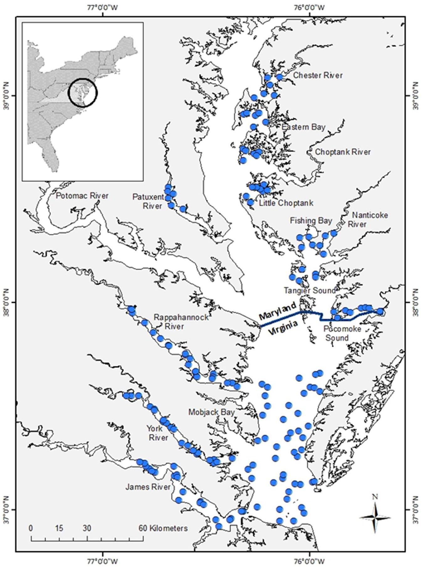
Figure 1. Sites (filled circles) sampled to assess relative abundance of forage fishes in Chesapeake Bay, 2000–2016. Sites in Virginia waters were sampled monthly from a random stratified survey design; sites depicted in the figure are from a representative month and year (October 2020). Fixed sites were sampled monthly between May and October in Maryland waters of Chesapeake Bay.

For each trawl tow, we expressed the relative index of abundance of juvenile (age-0) spotted hake, juvenile spot, juvenile weakfish, and all life stages of bay anchovy as the catch per unit effort (CPUE), where effort was estimated by the area swept by the net. Area swept was calculated by multiplying the geodetic distance of the tow by the effective net width, estimated as 55% of the headline spread based on gear tests performed in a flume tank. To relate forage fish abundance to suitable habitat areas and to ensure that CPUE best represented relative abundance, we restricted consideration of CPUE measures to those seasons in which individuals were available to the gear: spring (March, April, May) for juvenile spotted hake; summer (June, July, August) and fall (September, October, November) for juvenile spot and juvenile weakfish; and spring, summer, fall, and winter (December, January, February) for bay anchovy. Note that no sampling was completed in Maryland in winter, thus the bay anchovy CPUE index in winter was based on catches from Virginia waters only.

A Bayesian hierarchical method (Conn, 2010) was used to estimate baywide relative abundance for each species using the survey CPUEs. This method uses the coefficient of variation to weight the individual data sources and extracts a single annual index to represent the pattern exhibited by the multiple indices under the assumption that component indices are subject to process error (from variation in catchability, spatial distribution, etc.) and sampling error (i.e., within-survey variance; Conn, 2010). Annual baywide indices of relative abundance and their associated 95% credible intervals were estimated for the season(s) of interest for each forage species. We used WinBugs accessed through an R script (R Core Team, 2019) to perform these calculations.

Habitat Covariates

Static Habitat Covariates

Two static variables, distance to shore (km) and percent fine sediment, were determined for locations at the midpoint of each trawl tow (Table 1). Fringing marsh and other shallow water areas may provide resources that enhance survival and growth of forage fish (e.g., refuge from predators and provisioning of food; Manderson et al., 2004; França et al., 2009; Boutin and Targett, 2019), and as such, distance to shore may influence fish habitat use. The shortest distance to the nearest shoreline was calculated, and in some cases, the nearest shoreline was an in-Bay island (Figure 2A). Seabed percent fine sediment, a key feature of fish habitat (Kritzer et al., 2016), was determined from a baywide surface grain-size distribution map (Figure 2B) based on observed surface seabed grain size (Moncure and Nichols, 1968; Byrne et al., 1983; Kerhin et al., 1988; Velinsky et al., 1994; Maryland Geological Survey, 1996; Reid et al., 2005).

TABLE 1

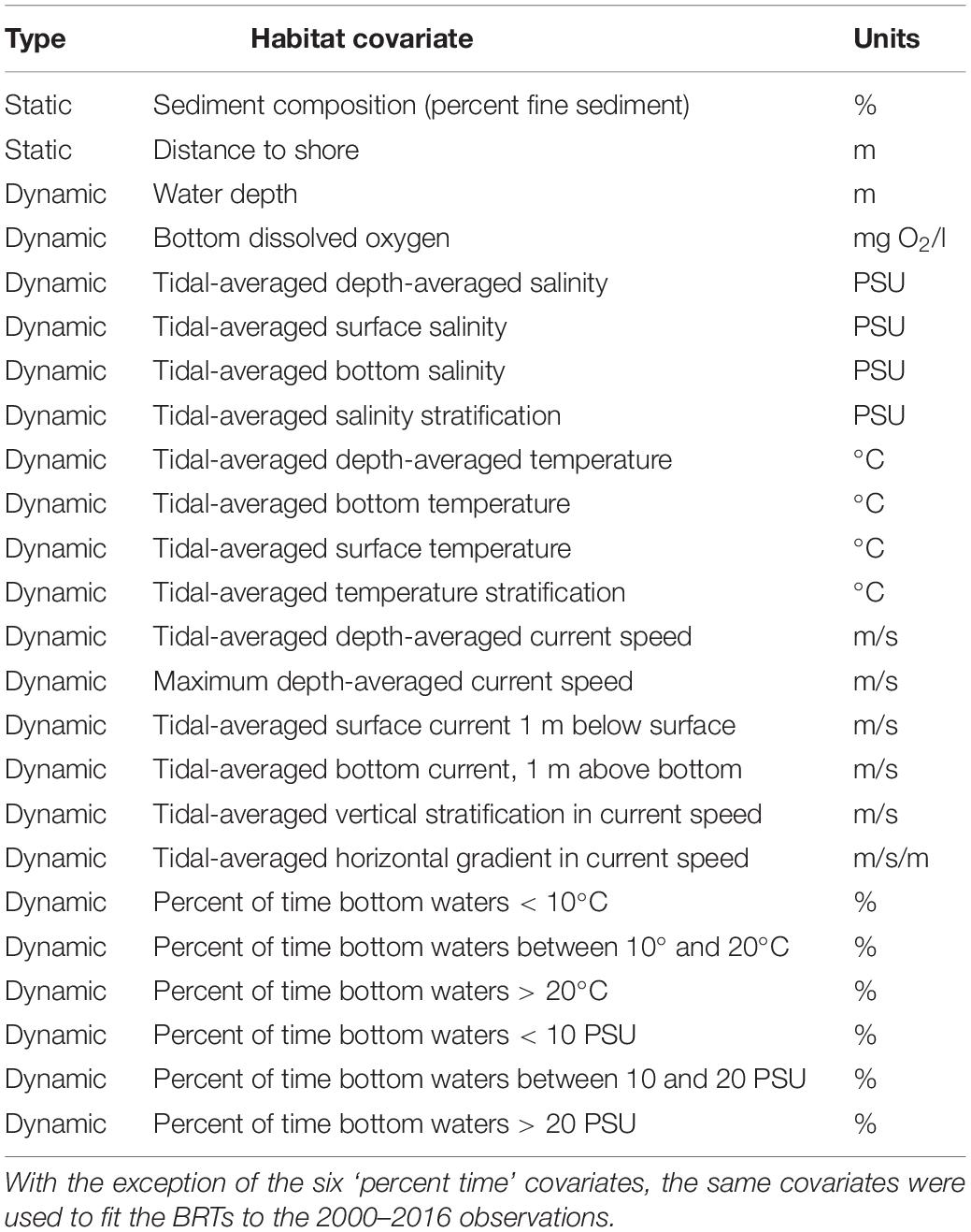
Table 1. Static and dynamic habitat features considered for optimization of boosted regression trees (BRTs) for forage fishes in Chesapeake Bay, 2010–2012.

FIGURE 2

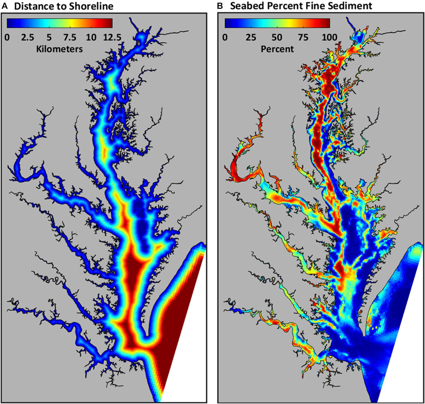
Figure 2. Distance to shoreline (km) (A) and sediment composition (% fines) (B) of the seabed in Chesapeake Bay.

Bottom-Water Dissolved Oxygen

Dissolved oxygen concentrations (mg O₂/l) were hindcast for bottom waters of the Chesapeake Bay and its tributaries using the methods of Du and Shen (2014) modified to include observations from monthly fisheries surveys, quarter-hourly records from Maryland data buoys (Maryland Eyes on the Bay), quarter-hourly records from the Virginia Estuarine and Coastal Observing System (VECOS), and monthly to bi-monthly surveys from the Chesapeake Bay Program’s Water Quality Monitoring Program. Monthly mean bottom DO conditions were calculated for each observed location in each year; we used these values at a 1-km² resolution to represent bottom DO conditions and then spatially interpolated values for grid cells that did not have estimated DO values. Using a 5-km search radius, we assigned bottom DO values to each 1-km² grid cell in one of two ways: if only a single grid cell in the search radius had an estimated DO value, that value was used; if more than one grid cell in the search radius had estimated DO values, then inverse distance weighting was used to obtain a value for the grid cell in question. The search expanded to 10 km in cases where no bottom DO values were available within 5 km. Daily interpolated bottom DO values were then estimated for 2000 to 2016 by linear regression through time in each grid cell using the monthly bottom DO values. Bottom DO observations from a subset of fisheries surveys (2010–2012; n = 4,604) used to develop the model revealed that at least 98% of hindcasts were reliable, that is, values in the normoxic range (DO > 5 mg O₂/l) were hindcast at 99% of locations where normoxic conditions were observed, and values indicating hypoxia (DO < 2 mg O₂/l) were hindcast at 98.4% of locations with observed hypoxic conditions.

Dynamic Habitat Covariates

Estimates of temperature, salinity, depth, and current speed were obtained from a three-dimensional model of the Chesapeake Bay developed using the UnTRIM hydrodynamic model (Casulli and Zanolli, 2002, 2005). This model takes advantage of the grid flexibility allowed in an unstructured mesh by gradually varying grid cell sizes, beginning with large grid cells in the Atlantic Ocean and transitioning to finer grid resolution in the smaller channels of the tributaries and the northern portion of the estuary (Figure 3). This approach allows for the model to accurately capture the bathymetry and shoreline at multiple spatial scales while maintaining suitable simulation times using a single high-end workstation computer. Further description of the inputs for the hydrodynamic model are provided in the Supplementary Material, along with a summary of the model validation to the data most relevant to this study. This validation demonstrated that the model accurately estimated temperature and salinity in the Bay and major tributaries under a wide range of environmental conditions (Supplementary Figures 1, 2); model accuracy was similar to that reported for a suite of Chesapeake Bay models evaluated by Irby et al. (2016).

FIGURE 3

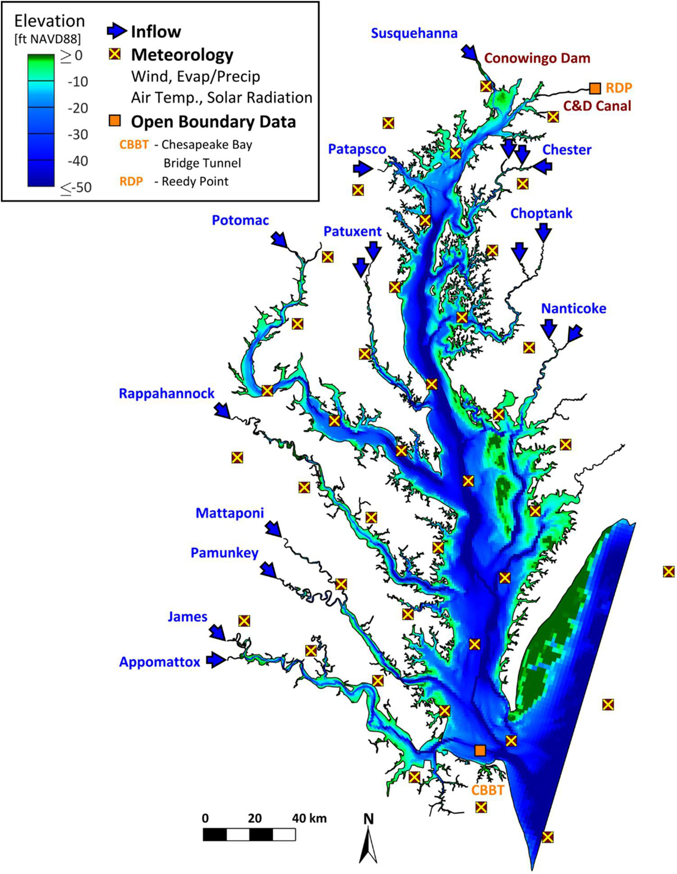
Figure 3. Model domain and boundary conditions for the 3-dimensional UnTRIM Chesapeake Bay model used to hindcast dynamic environmental conditions for forage fishes, 2000–2016.

A large number of environmental variables were initially considered for use in developing fish habitat suitability models to eliminate a priori specification of environmental conditions that may be important for describing abundance and distribution of forage fishes. Twenty-two dynamic environmental variables were calculated, along with sediment composition and distance to shore (Table 1). Environmental covariates were extracted from the hydrodynamic model and the DO model at the time and location of the individual tows (midpoint of the tow) to allow us to couple fisheries observations with hindcasts of environmental covariates. We considered hindcasts of environmental covariates at multiple temporal and spatial scales because such measures may provide more accurate predictions of habitat suitability (Lecours et al., 2015). Dynamic variables were extracted from the hydrodynamic model as instantaneous values at the time of each tow (i.e., the time of capture), and as the tidal-averaged (24.8 h) values in the tidal cycle preceding the capture event. Conditions preceding capture may influence the distribution of fishes (e.g., Jaonalison et al., 2020), and preliminary investigations with boosted regression trees suggested that models that considered tidal-averaged conditions performed better than those with comparable instantaneous values; henceforth, we considered tidal-averaged conditions. Depth-averaged conditions were obtained for salinity, temperature, and current speed (Table 1). Tidal-averaged current speeds provide a metric of flow which may be used by some species to aid movements within the estuary (Brady and Targett, 2013). We also considered covariates describing near-bed conditions (1 m above the seabed), and maximum depth-averaged current speed. Because vertical or horizontal gradients in current speed may act to aggregate food near complex currents or fronts, we also considered these covariates. The vertical gradient in the current speed was calculated as the difference between the current speed one meter above the bottom and one meter below the surface; the horizontal gradient in the current speed was calculated as the maximum difference in current speed between adjacent model grid cells divided by the distance between the model grid cells.

Although habitat conditions near the seabed may be most relevant for understanding fish-habitat relationships for demersal species such as spotted hake, habitat use may also reflect overall conditions in the water-column because even demersal fishes are not confined to near-bed habitats. For example, salinity stratification may influence the supply of food or DO to the near-bed region sampled by the trawl, and may be an indicator of forage fish occurrence. Thus, we used covariates describing salinity and temperature stratification, that were calculated as the difference between instantaneous surface (top 1 m) and near-bed (1 m above seabed) conditions. In addition, because favorable habitats may be characterized by a range of conditions, we considered covariates based on the percent of time that near-bed conditions fell within a given range, for example, the percent of time that salinity exceeded 20 PSU. The percent of time within a given salinity or temperature range was calculated over the same time interval used for tidal averaging. We identified three salinity ranges (<10 PSU; 10–20 PSU; >20 PSU), and three temperature ranges (<10°C; 10–20°C; >20°C) consistent with observed patterns in fish communities in Chesapeake Bay (Tuckey and Fabrizio, personal observation).

Selection of Influential Habitat Covariates

Boosted regression trees (BRTs) were used to select a subset of influential habitat covariates that explained variations in the nominal catch rates of fish (Breiman et al., 1984). The regression tree algorithm uses recursive partitioning to explain variation in the response (nominal catch rates), that is, observations are repeatedly split into increasingly homogeneous groups based on threshold values of the predictors (habitat covariates; Breiman et al., 1984). Cross-validation was used to assess model fit and to ensure that the resultant trees were applicable to out-of-sample observations; cross-validation was achieved by fitting the tree to a subset of the data (the training set) and fit was assessed using the remaining data (the test set). Furthermore, the performance of regression tree algorithms may be improved with ensemble methods such as boosting, which aggregates multiple trees to enhance the stability of the resultant model (Knudby et al., 2010). We used a Poisson response to model the number of fish captured per tow with the gbm.step procedure (R package ‘dismo,’ Elith et al., 2008; Elith and Leathwick, 2017; R Core Team, 2019). Catches from the Virginia survey were used without modification (numbers per 5-min tow), but catches from the Maryland survey were expressed in 5-min-tow equivalencies rounded to the nearest integer. All habitat covariates were standardized to permit direct comparison of covariate importance (Schielzeth, 2010).

Optimization of Boosted Regression Tree Models

Prior to fitting the BRTs to the 2000–2016 observations, we optimized the model-fitting parameters of the BRTs by exploring the combination of parameter values that produced the lowest deviance of the cross-validated data sets (Elith et al., 2008; Cameron et al., 2014). To determine optimal parameters values for the BRTs and because optimization is computationally intensive, we used a subset of observations (2010–2012; n = 4,604 tows) that represented notably different environmental conditions (2011 was a wet year compared with 2010) as well as large differences in the observed relative abundance of forage species. BRT parameters were optimized separately for spotted hake, spot, weakfish, and bay anchovy using the gbm.step procedure in R (dismo package, R Core Team, 2019). Model fitting failed to produce at least 1,000 trees for bay anchovy using all of the 2010-2012 observations, so we optimized BRT parameters using data from each season separately. For bay anchovy in fall, BRT modeling yielded less than 1,000 trees and was thus unreliable (Elith et al., 2008) and not considered further.

Optimization focused on selection of the learning rate and tree complexity, two model-fitting parameters assigned by the analyst. The learning rate determines how quickly the model approximates the observed data (Miller et al., 2016), and the tree complexity represents the level of interaction possible among the predictors. The third parameter selected by the analyst is the bag fraction, or the proportion of observations used to train the model. Observations in the training subset are selected randomly without replacement for each model run and the remaining observations are used for cross-validation. Preliminary investigations suggested that a bag fraction of 0.75 was reasonable. Using this bag fraction, we fitted a series of trees to a range of learning rates (lr = 0.0005, 0.0050, 0.0075, 0.0100, 0.0200, 0.0300, 0.0400, 0.0500, 0.0750) and tree complexities (tc = 1, 3, 5, 10), similar to Cameron et al. (2014). For each species, we considered only those BRTs for which at least 1,000 trees were fit and selected parameter values that reduced the cross-validated deviance (Elith et al., 2008). We identified the optimal tree complexity for each species by graphically examining the change in cross-validated deviance across learning rates. Next, using the selected tree complexity, we identified the learning rate that produced the minimum cross-validated deviance.

To select influential habitat covariates, we fitted BRT models for each species for the period 2000–2016 (N_total = 25,333 tows; N_Virginia = 20,326 tows, N_Maryland = 5,007 tows) using a bag fraction of 0.75 and values of the optimized species-specific learning rates and tree complexities determined by optimization. Optimized model-fitting parameters (lr and tc) varied among species: juvenile spotted hake lr = 0.01 and tc = 10; juvenile spot lr = 0.02 and tc = 10; juvenile weakfish lr = 0.005 and tc = 10; and bay anchovy (spring, summer, winter) lr = 0.02 and tc = 3. In addition, optimization runs indicated that the six covariates describing percent time were least informative, so these were not considered further. Therefore, a suite of 18 covariates (16 dynamic, 2 static; Table 1) were considered for the BRT models. Estimates of variable influence and scree plots produced by the gbm.step procedure (R Core Team, 2019) allowed us to identify and select a subset of influential covariates for each species, and for bay anchovy for each season (spring, summer, winter). Care was taken to consider only those covariates that did not exhibit high correlations with other influential covariates, that is, only those covariates with r² < 0.8 were considered in the subsequent calculation of habitat suitability indices (HSIs). This approach avoids overweighting of the HSI for a particular habitat condition.

Habitat Suitability Models

Habitat suitability models were used to assign habitat suitability scores and to quantify the extent of suitable habitat for forage fishes throughout the Chesapeake Bay and its tributaries from 2000 to 2016 for each season. Habitat suitability models were estimated with the non-parametric histogram approach because this approach makes no assumption about the nature of the relationship between environmental features and fish abundance (Guan et al., 2016). Briefly, thresholds of environmental conditions that resulted in a gradient of suitability from least suitable (0) to most suitable (1) were identified for each influential habitat covariate for each species. The HSI, calculated as the mean of two or more covariate-specific suitability indices (SIs), also ranged between 0 and 1 to ease interpretation.

Suitability Indices

We estimated SIs for the range of observed values for each of the influential habitat covariates identified by the species-specific BRTs. We used the Tanaka and Chen (2015) approach to estimate SIs but applied a disjoint clustering method to identify ‘natural clusters’ of the habitat covariates for the histogram approach; we implemented this method with the FastClus procedure in SAS/STAT^®. Tanaka and Chen (2015) fixed the number of individual bins to 10 for each habitat covariate, but we found that this resulted in bins with few observations (<5) or narrowly defined environmental limits (e.g., bottom temperature between 16.2 and 16.3°C). Thus, we allowed the number of bins to vary (but not exceed 10), and restricted cluster sizes to a minimum of 40 observations; in all cases, the smallest cluster included at least 54 observations, allowing a reasonable description of average abundance (and hence, relative suitability) in each cluster. SIs were estimated for each cluster and habitat covariate using

$$S{I}_{ij}=\frac{CPU{E}_{ij}-CPU{E}_{i,\min }}{CPU{E}_{i,\max }-CPU{E}_{i,\min }}$$

where SI_ij is the suitability index for cluster j of habitat covariate i, CPUE_ij is the average catch (fish/km²) observed in cluster j of habitat covariate i, and CPUE_i,min and CPUE_i,max are the minimum and maximum average catches observed across all clusters of habitat covariate i (Tian et al., 2009; Chang et al., 2012). This formulation allows the SIs to range between 0 and 1.0, with 1.0 indicating the most suitable condition and 0 the least. More explicitly, each covariate cluster, defined by a range of values, was associated with an SI score.

Habitat Suitability Indices

Habitat suitability indices were calculated by expressing the HSI as an average of multiple covariate-specific SIs; we restricted the number of covariates in the HSI to those that were most influential as determined by BRTs (Table 2). The HSI for a given set of covariates may be expressed as an arithmetic or geometric mean of the individual SIs (e.g., Brown et al., 2000; Tanaka and Chen, 2015). A single averaging approach to estimate the HSIs, however, may not be appropriate for all species (e.g., Yu et al., 2019), so we explored both models of the mean. The arithmetic mean model for the HSI is

$$HS{I}_{am}=\frac{S{I}_1+S{I}_2+S{I}_3+\mathrm{\cdots }S{I}_p}{p}$$

TABLE 2

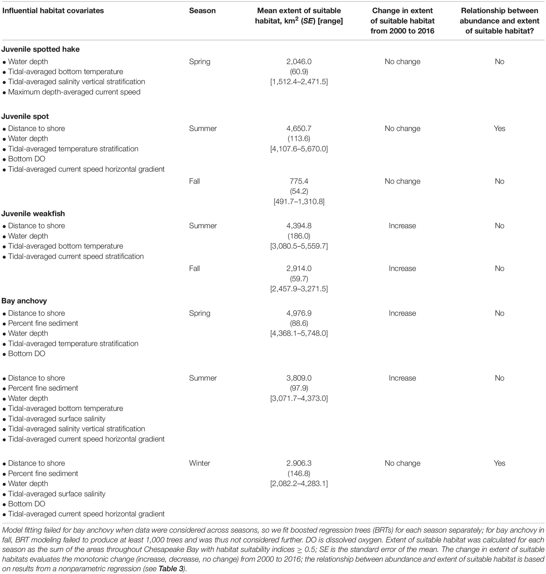
Table 2. Summary of key results for juvenile spotted hake, juvenile spot, juvenile weakfish, and bay anchovy from Chesapeake Bay, 2000–2016; only those seasons during which fish were available to the gear are shown.

where SI₁ is the suitability index for habitat covariate 1, SI₂ is the suitability index for covariate 2, and so forth; and p is the number of covariates considered (e.g., Hess and Bay, 2000). The geometric mean model for the HSI is

$$HS{I}_{gm}=\sqrt[p]{S{I}_1\times S{I}_2\times S{I}_3\times \mathrm{\cdots }S{I}_p}$$

(e.g., Layher and Maughan, 1985; Lauver et al., 2002; Tian et al., 2009). The geometric mean index applies the concept of a ‘limiting factor’ whereby a low SI for a single covariate results in a low HSI_gm (Zajac et al., 2015). HSI calculations were performed in SAS^® or Matlab (MathWorks Inc.).

Habitat suitability index models were calibrated by using fish catches at each tow location and graphically examining the relationship between the HSIs and the average relative abundance for each species-season combination (e.g., Tanaka and Chen, 2015). We used the 5% trimmed mean as a measure of the average because trimmed means are insensitive to the occasional extreme catches observed for some species. For a properly calibrated HSI, the mean relative abundance of forage fish is expected to increase as habitat conditions approach optimal for the species, that is, as the HSI increases from 0 to 1.0.

Verification of Modeling Approach

We verified the use of BRTs for selection of covariates and evaluated the reliability of the two averaging formulations of HSI for forage fishes using bootstrap resampling (Efron and Tibshirani, 1986). About 70% of the fisheries observations (N = 18,121) comprised the training data set, and the remaining ∼30% (N = 7,212) was used as the test (or verification) data set. The SurveySelect procedure in SAS/STAT^® was implemented to randomly select samples without replacement using a stratified design to ensure representation across years, seasons, and geographic areas (Maryland and Virginia). Training and test data sets were constructed separately for each species, and bay anchovy sets were constructed separately for spring, summer, and winter. For each training data set, we fitted BRTs using the same bag fraction and species-specific lr and tc as before; we then selected influential covariates, and modeled the HSI_am and HSI_gm. Note that the BRTs for each data set may have indicated a different number of influential covariates, as well as a different suite of influential covariates, than what was identified by the original BRT model fitted to observations from 25,333 tows. The resulting HSI models were applied to each of the test data sets to estimate the predicted HSIs. Due to computational intensity, 10 cross-validation data sets were generated (consistent with Pennino et al., 2020). The expected performance of the HSI_am and HSI_gm for each species across all seasons was evaluated with the root mean square error (RMSE), calculated as the standard deviation of the residuals (where residuals represent the difference between the predicted HSI and observed HSI for each location where fish were sampled). For bay anchovy, we estimated RMSEs for spring, summer, and winter individually. We used a paired t-test implemented in the glm procedure in SAS^® to assess differences in mean RMSEs, and retained the HSI formulation that exhibited the lower mean RMSE for further analyses.

Estimation of the Extent of Suitable Habitat

The extent of suitable habitat for each species was quantified (objective 1) by calculating HSIs from the environmental covariates at each hydrodynamic model grid cell for each season from 2000 through 2016. To facilitate GIS visualization of seasonal habitat conditions and calculation of the area of suitable habitat for each species, we used the median of the daily values of the covariates to represent the seasonal average for a given model grid cell, season, and year. Median values for each habitat covariate at each model grid cell were then used to estimate the HSIs for each species. In this manner, we mapped the species-specific seasonal HSIs at the spatial resolution of the hydrodynamic model because processes operating at small spatial scales may be masked when environmental conditions are averaged over large spatial scales (Windle et al., 2012). The areas of the individual grid cells where HSI exceeded a given threshold of suitability (i.e., HSI ≥ 0.5, HSI ≥ 0.6, HSI ≥ 0.7, HSI ≥ 0.8) were summed to obtain an estimate of the extent of ‘suitable’ habitat throughout the Chesapeake Bay and its tributaries for each species, season, and year. Preliminary graphical investigations revealed that annual patterns in suitable habitat extents were similar among the 0.5, 0.6, and 0.7 thresholds; the 0.8 threshold yielded values that were too low to be useful. The 0.5 threshold, used to describe habitat suitability for the eastern oyster Crassostrea virginica in Chesapeake Bay (Theuerkauf and Lipcius, 2016) and for pelagic sharks in Australia (Birkmanis et al., 2020), was used for subsequent analyses and presentation.

Relationship Between Suitable Habitat Extent and Relative Abundance of Forage Species

We hypothesized that annual and seasonal changes in the area of suitable habitat affect the abundance of forage species in this temperate ecosystem. To address this hypothesis, we related the annual time series of suitable habitat with annual estimates of baywide relative abundance for each species (objective 2). We limited the exploration of these relationships to the season during which a particular species was most vulnerable to the trawl gear: juvenile spotted hake in spring, juvenile spot in summer and fall, juvenile weakfish in summer and fall, and bay anchovy in spring, summer, and winter. We rank transformed abundance indices because of the small number of observations (n = 17 years except for bay anchovy in winter when n = 16) and fit non-parametric regressions to model the relationship between rank abundance and extent of suitable habitat. For this analysis, we assumed the relationship was stationary, that is, the effect of suitable habitat extent on the abundance of forage fishes remained stable from 2000 to 2016 (e.g., Zeng et al., 2018). In addition, we tested the null hypothesis that the seasonal extent of suitable habitat was constant in Chesapeake Bay between 2000 and 2016; as before, we rank transformed the extent of suitable habitat (defined as areas with HSI ≥ 0.5). Computations for non-parametric regression analyses were performed with the rank and glm procedures in SAS^®. Residual plots indicated a reasonable fit of the rank regression model to the data.

Results

Influential Habitat Covariates

Environmental conditions and habitat features that comprised suitable habitats varied among species and ranged between four and seven, depending on species (Table 2). Water depth and one of the current speed metrics were consistently identified as influential covariates for all species; one of the temperature covariates was influential in describing suitable habitats for forage fishes in spring, summer, and fall, but was not selected for describing suitable habitats in winter (Table 2). At least one salinity metric defined suitable habitats for juvenile spotted hake and bay anchovy, and distance to shore explained suitable habitats for juvenile spot, juvenile weakfish, and bay anchovy (Table 2). Bottom DO conditions delineated suitable habitats for juvenile spot in winter and bay anchovy in winter and spring (Table 2). Conditions at sites sampled in Maryland waters differed from those in Virginia waters: in Maryland, sampled habitats tended to be shallower, closer to shore, warmer in summer, and cooler in fall than habitats sampled in Virginia (Supplementary Figure 3). Most notably, Maryland sites exhibited lower bottom DO concentrations in summer than Virginia sites (Supplementary Figure 3). In addition, relative to sites in Virginia, Maryland sites exhibited lower surface salinities, less stratification in terms of salinity and temperature, lower current speeds and less stratification in current speeds (Supplementary Figure 3).

Verification and Calibration of the Habitat Suitability Index Modeling Approach

Bootstrap analyses verified that BRTs were useful for selection of influential covariates; in general, the same or similar covariates were identified as most influential among the 10 bootstrap realizations. For juvenile spotted hake, the HSI formulation based on the geometric mean (HSI_gm) provided the best approximation to the original HSI estimated for each sample as indicated by the significantly lower RMSE (t = 4.56, P < 0.01). Unlike results for juvenile spotted hake, the HSI based on the arithmetic mean (HSI_am) performed better for bay anchovy, regardless of season (t_spring = –3.08, P_spring < 0.01; t_summer = –4.01, P_summer < 0.01; t_winter = –3.27, P_winter < 0.01). Although we found no evidence for a difference in the mean RMSEs of the HSI_am and the HSI_gm for juvenile spot and juvenile weakfish (t_spot = –1.13, P = 0.27; t_weakfish = –1.65, P = 0.12), we used the HSI_am for these species because the mean RMSE of the HSI_am was consistently less than the mean RMSE of the HSI_gm.

Relative abundance as measured by the trimmed mean of the four species increased with increasing values of HSIs (Figure 4), indicating proper calibration of habitat suitability models. The ranges of observed HSI values across years were 0–0.95 for juvenile spotted hake in spring; 0.12–0.98 for juvenile spot in summer; 0.04–0.86 for juvenile spot in fall; 0.09–0.99 for juvenile weakfish in summer; 0–0.89 for juvenile weakfish in fall; 0–0.92 for bay anchovy in spring; 0–0.92 for bay anchovy in summer; and 0.04–0.98 for bay anchovy in winter.

FIGURE 4

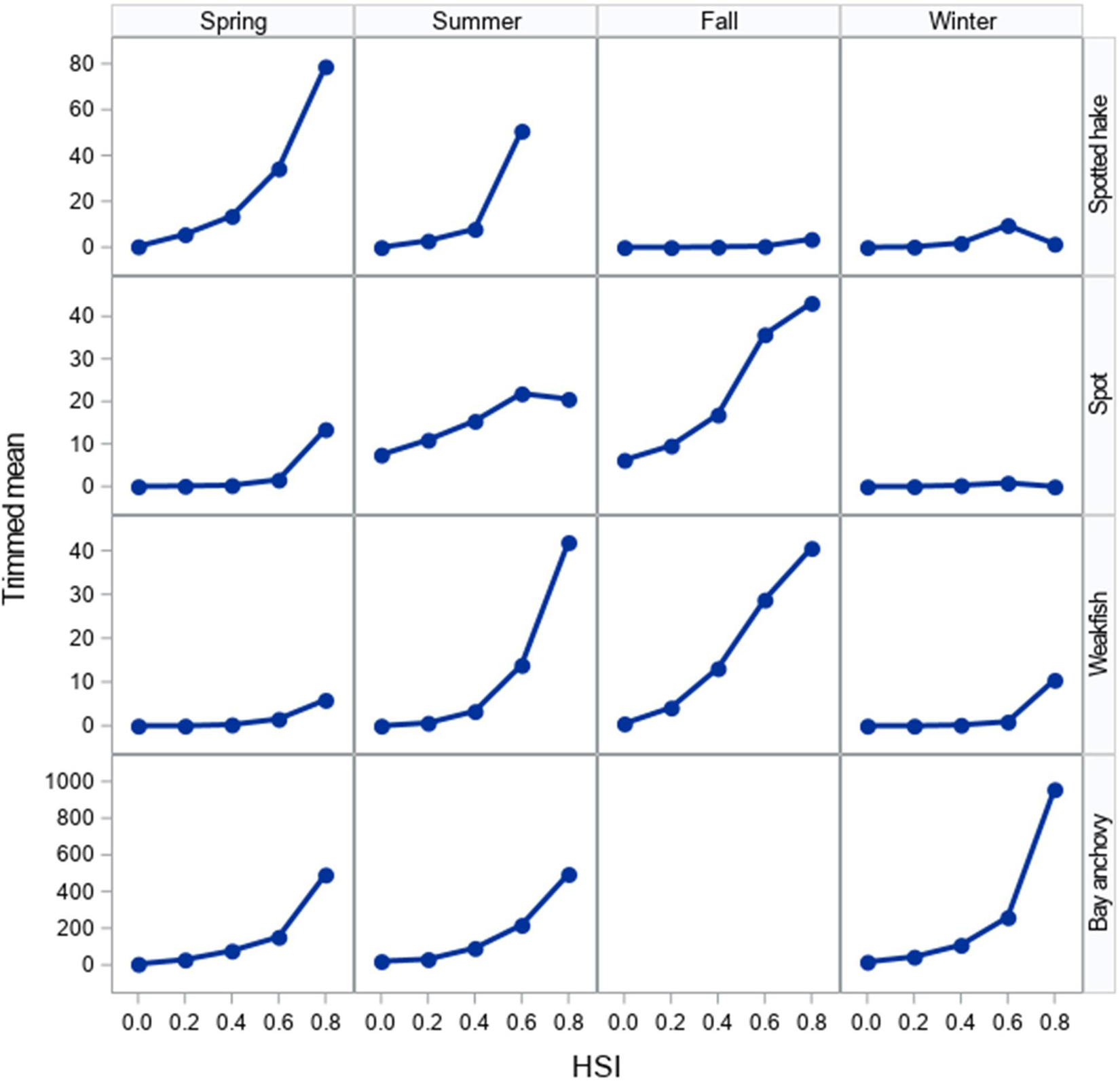
Figure 4. Relationship between HSI and trimmed mean catches of juvenile spotted hake, juvenile spot, juvenile weakfish, and bay anchovy in Chesapeake Bay, 2000–2016. For juvenile spotted hake, the HSI_gm is shown, whereas the HSI_am is shown for other species. HSI values were binned for ease of plotting such that bin 0.0 includes all observations where 0 ≤ HSI < 0.2, bin 0.2 includes all observations where 0.2 ≤ HSI < 0.4, and so forth. Note differences in y-axes.

Suitable Habitat Extent for Forage Fishes

Juvenile Spotted Hake

We detected a strong seasonal pattern in the extent of suitable habitats for juvenile spotted hake in Chesapeake Bay: little to no suitable habitat was available in summer and fall, increased in winter (mean_winter = 467.0 km² or 4.3% of the total area modeled), and was greatest in spring (mean_spring = 2,046.0 km² or 18.8% of the total area; Table 2, Figure 5A, and Supplementary Figure 4A). In spring, the extent of suitable habitat was greater in the Virginia portion of the Chesapeake Bay system than in the Maryland portion (Supplementary Figure 5A). Suitable habitats for spotted hake in spring were relatively deep, away from shorelines, and where salinity stratification was greater than 4.9 psu (Figure 5A); these habitats were characterized by tidal-averaged bottom temperatures ranging between 5.3 and 14.2°C. Annual changes in the extent of suitable habitats varied by as much as 90.3% in winter (Figure 6A) and as much as 38.8% in spring (Figure 6B) across the time period of study. The extent of suitable winter habitat was higher during years when waters in the region began to warm earlier in the year (e.g., 2012) and was lower when warming was delayed (e.g., 2011; Figure 6A).

FIGURE 5

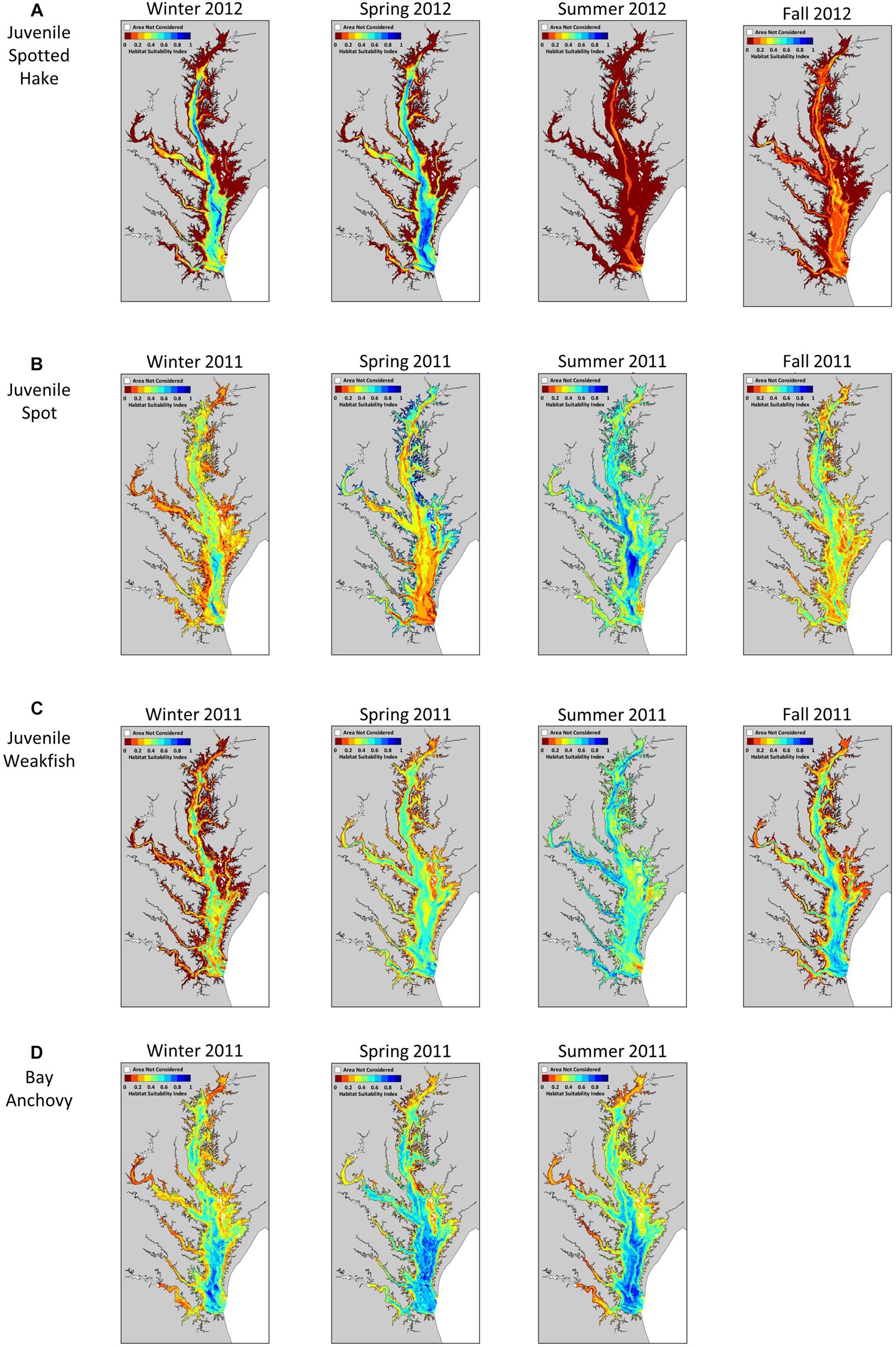
Figure 5. Representative examples of seasonal variation in habitat suitability for (A) juvenile spotted hake, (B) juvenile spot, (C) juvenile weakfish, and (D) bay anchovy in Chesapeake Bay. The habitat suitability index ranges from 0 (red) indicating poor habitat to 1 (blue) indicating most suitable habitat.

FIGURE 6

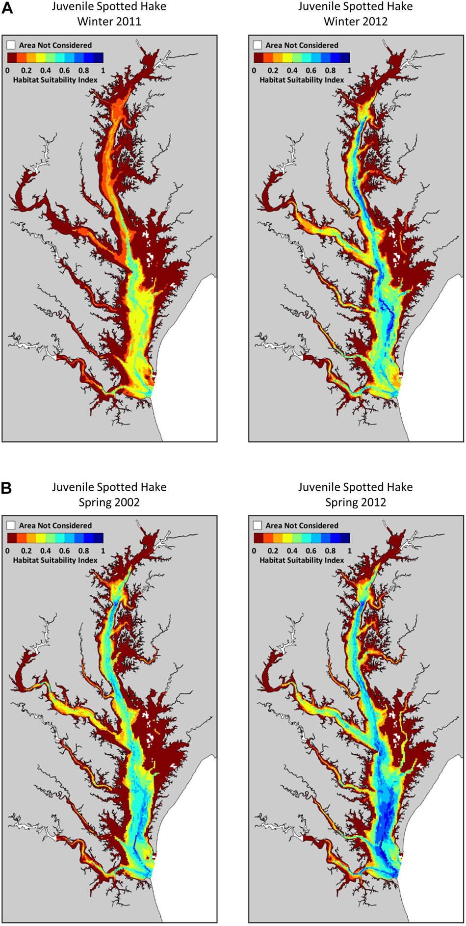
Figure 6. Annual variation in extent of suitable habitats for juvenile spotted hake in Chesapeake Bay: (A) winter 2011 vs. 2012 (90.3% increase), and (B) spring 2002 vs. 2012 (38.8% increase). The habitat suitability index ranges from 0 (red) indicating poor habitat to 1 (blue) indicating most suitable habitat.

Juvenile Spot

The extent of suitable habitat for juvenile spot displayed a persistent seasonal pattern, with relatively greater extents of suitable habitats in spring (mean_spring = 3,169.4 km² or 29.1% of the total area) and summer (mean_summer = 4,650.7 km² or 42.6% of the total area) and relatively little suitable habitat in fall and winter (mean_fall = 775.4 km² or 7.1% of the total area; mean_winter = 864.0 km² or 7.9% of the total area; Table 2, Figure 5B, and Supplementary Figure 4B). Suitable habitats for juvenile spot were primarily found in shallow areas near shorelines in spring, and in the deeper portions of the Chesapeake Bay and its tributaries in summer (Figure 5B). In tributaries and embayments such as Mobjack Bay, the extent of suitable habitat for juvenile spot in spring was greater than that in summer by as much as 47.2%. Suitable habitat extents in spring and summer were greater in the Maryland portion of the Chesapeake Bay system compared with the Virginia portion (Supplementary Figure 5B). The extent of suitable habitats for spot was driven by distance to shore, depth, temperature stratification, bottom DO, and horizontal gradients in current speed, and was not well described by a single covariate (Table 2). Nevertheless, suitable habitats exhibited bottom DO levels less than 4.0 mg O₂/l in summer and less than 5.3 mg O₂/l in fall, suggesting that juvenile spot used habitats that may be considered marginal or unsuitable for other species. Low bottom DO conditions are associated with stratified water column conditions and indeed, juvenile spot were more likely to occur in habitats where tidal-averaged temperature stratification exceeded 2.2°C in summer and 2.7°C in fall.

Juvenile Weakfish

A notable seasonal pattern was evident in the amount of suitable habitat available for juvenile weakfish: little suitable habitat was available in winter (mean_winter = 667.3 km² or 6.1% of the total area), increased in spring (mean_spring = 2,446.3 or 22.4% of the total area) and was greatest in summer (mean_summer = 4,394.8 or 40.3% of the total area; Table 2, Figure 5C, and Supplementary Figure 4C). Throughout the Chesapeake Bay system, the extent of suitable habitat in fall was, on average, 19.1% greater than in spring, but this pattern was not observed in 2000, 2010, and 2012 (Supplementary Figure 4C). In summer, suitable habitats for juvenile weakfish were found close to shorelines; in fall, suitable habitats were away from shore, near the mouth of the Potomac River and the lower Chesapeake Bay (Figure 5C). In Virginia waters, we observed similar extents of suitable habitats in summer (mean_summer = 2,056.7 km² or 18.9% of the total area) and fall (mean_fall = 2,007.7 km² or 18.4% of the total area), but in Maryland waters, suitable habitat extents declined by an average of 61.2% from summer (mean_summer = 2,338.0 km² or 21.4% of the total area) to fall (mean_fall = 906.3 km² or 8.3% of the total area; Supplementary Figure 5C). Regional differences in fall were clearly depicted by seasonal maps: HSI values in the mainstem of the bay were greater in waters south of the Rappahannock River than north of the Rappahannock River (Figure 5C). Suitable habitats for juvenile weakfish were characterized by distance to shore, depth, bottom temperature, and current speed stratification (Table 2).

Bay Anchovy

The estimated extent of suitable habitat for bay anchovy varied seasonally, with the greatest extent of suitable habitat area in the Chesapeake Bay system in spring (mean_spring = 4,976.9 km² or 45.6% of the total area), followed by summer (mean_summer = 3,809.0 km² or 34.9% of the total area) and winter (mean_winter = 2,906.3 km² or 26.6% of the total area; Table 2, Figure 5D, and Supplementary Figure 4D). Although this seasonal pattern was also observed for Virginia waters (mean_spring = 3,117.2 km² or 28.6%; mean_summer = 2,774.4 km² or 25.4%; mean_winter = 1,839.8 km² or 17.0%), suitable habitat extents in Maryland waters were greatest in spring (mean_spring = 1,859.7 km² or 17.0%) and lower but similar in summer and winter (mean_summer = 1,034.6 km² or 9.5%; mean_winter = 1,066.5 km² or 9.8%; Supplementary Figure 5D). The greatest extents of suitable habitats in tributaries occurred in spring; in summer and winter, the upper reaches of major tributaries were particularly unsuitable for bay anchovy (Figure 5D). Suitable habitat conditions occurred in areas that reflected complex relationships between multiple environmental and geophysical covariates and consistently included sediment composition, depth, and distance to shore.

Relative Baywide Abundance and Relationship to Extent of Suitable Habitat

Seasonal indices of relative abundance for forage fishes in Chesapeake Bay varied across years, and interannual patterns were generally similar for the Virginia and Maryland surveys, particularly for juvenile spotted hake in spring, juvenile spot in summer and fall, and juvenile weakfish in summer (Figure 7). Inconsistent patterns in interannual changes in relative abundance between Virginia and Maryland waters were observed for juvenile weakfish in fall and bay anchovy in spring and summer (Figure 7), suggesting that seasonal processes affecting the distribution of these species varied across regions of the Chesapeake Bay. We note that the mean index of relative abundance for juvenile weakfish in fall was several orders of magnitude lower in Maryland waters than in Virginia. Similarly, the mean indices of relative abundance for bay anchovy in spring and summer were an order of magnitude lower in Maryland waters than in Virginia. Spatial differences in relative abundance reflected the geographic differences in the extents of suitable habitats which were notably lower in Maryland than in Virginia for these species-season combinations (Supplementary Figures 5C,D).

FIGURE 7

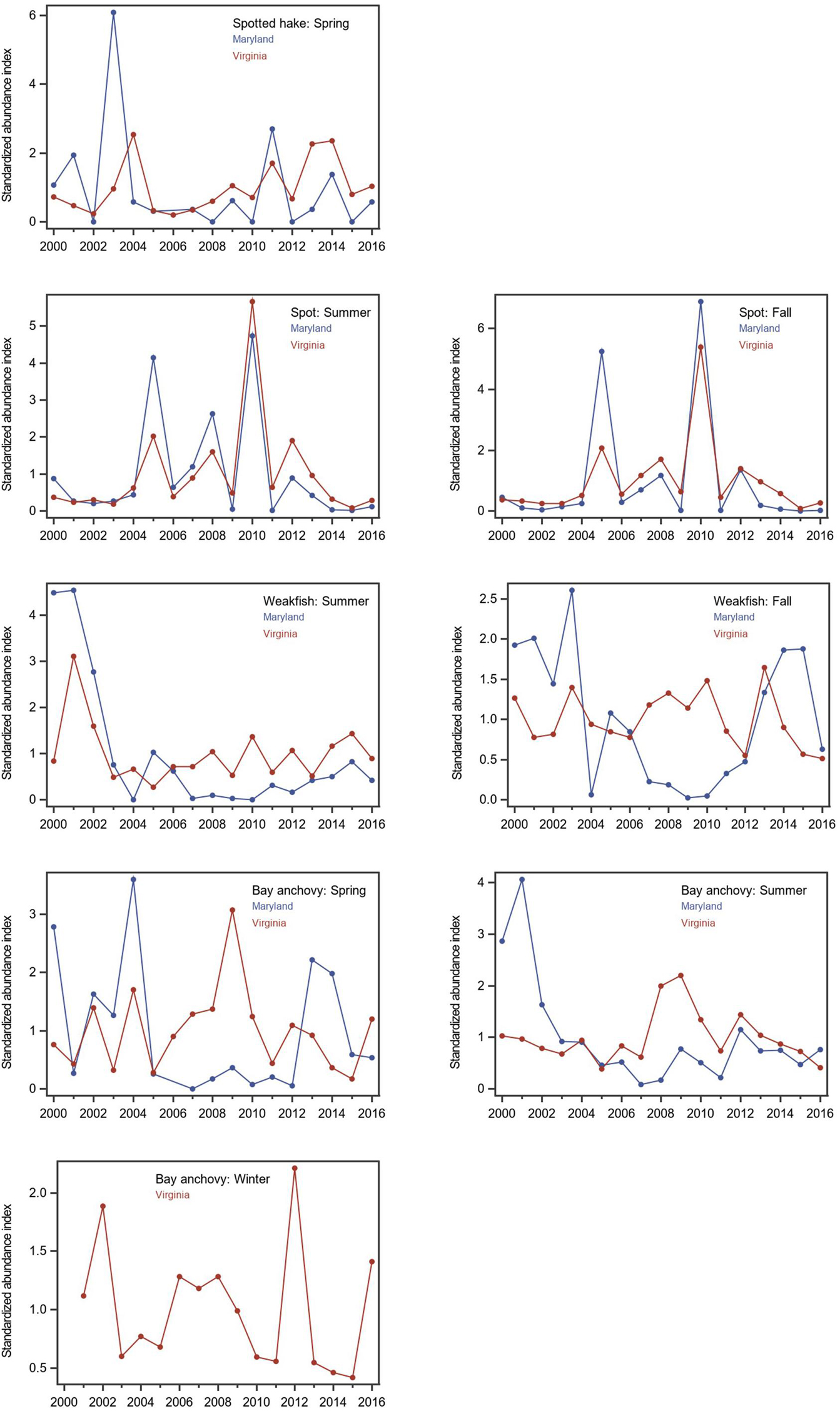
Figure 7. Seasonal standardized abundance indices for forage fishes in Maryland (blue) and Virginia (red) waters of Chesapeake Bay, 2000–2016: juvenile spotted hake in spring, juvenile spot in summer and fall, juvenile weakfish in summer and fall, and bay anchovy in spring, summer, and winter. Seasons were March–May for spring, June–August for summer, September–November for fall, and December–February for winter. Seasonal relative abundance indices (mean catch per unit effort expressed as number of fish/km²) were standardized to a mean of 1.0 across the 17 years, thus, patterns of abundance can be compared between states, but these standardized abundance indices do not reflect differences in estimated mean catch rates within a given year. Note that bay anchovy were not sampled in Maryland in winter, and thus, only the standardized index for Virginia is depicted.

Two contrasting relationships were detected between the ranked baywide relative abundance index and the extent of suitable habitat for forage fishes. We observed a significant positive relationship between seasonal ranked baywide relative abundance and extent of suitable habitat for juvenile spot in summer (Tables 2, 3 and Figure 8A). The baywide relative abundance index for juvenile spot in summer was highly variable with contrasting periods of low and high abundance (Figure 9A). Extents of suitable summer habitat for juvenile spot exhibited no significant linear pattern across time (Tables 2, 3 and Figure 9A). We observed a similar relationship for bay anchovy in winter: the extent of suitable habitat in winter was a significant determinant of the ranked relative abundance of bay anchovy (Table 3 and Figure 8B). The baywide relative abundance of bay anchovy varied widely in winter and exhibited no obvious temporal pattern (Figure 9B); extents of suitable winter habitat for bay anchovy showed no systematic change through time (Tables 2, 3 and Figure 9B).

TABLE 3

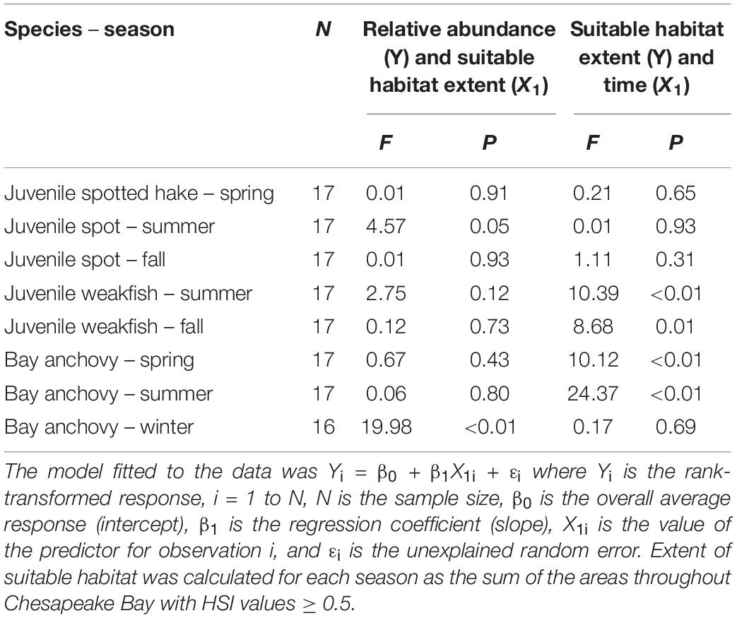
Table 3. Non-parametric regression analysis results for juvenile spotted hake, juvenile spot, juvenile weakfish, and bay anchovy from Chesapeake Bay, 2000–2016.

FIGURE 8

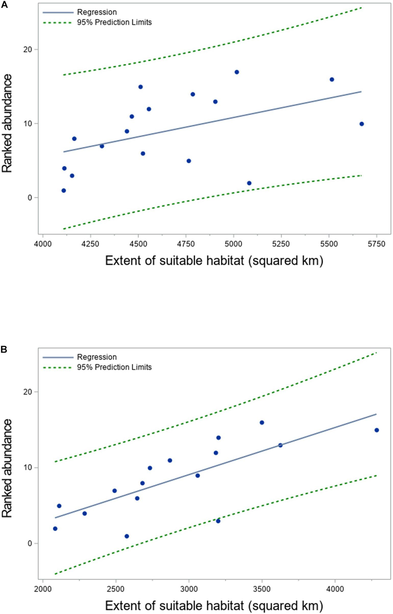
Figure 8. Non-parametric relationship between rank abundance and extent of suitable habitat (km²) for (A) juvenile spot in summer and (B) bay anchovy in winter in Chesapeake Bay, 2000–2016. Observations are depicted by filled circles; the solid line is the nonparametric regression fit to the observations, and the dashed line is the 95% prediction limit. The Spearman correlation coefficients were 0.54 for spot in summer and 0.80 for bay anchovy in winter. Values of HSI_am ≥ 0.5 were considered suitable habitat.

FIGURE 9

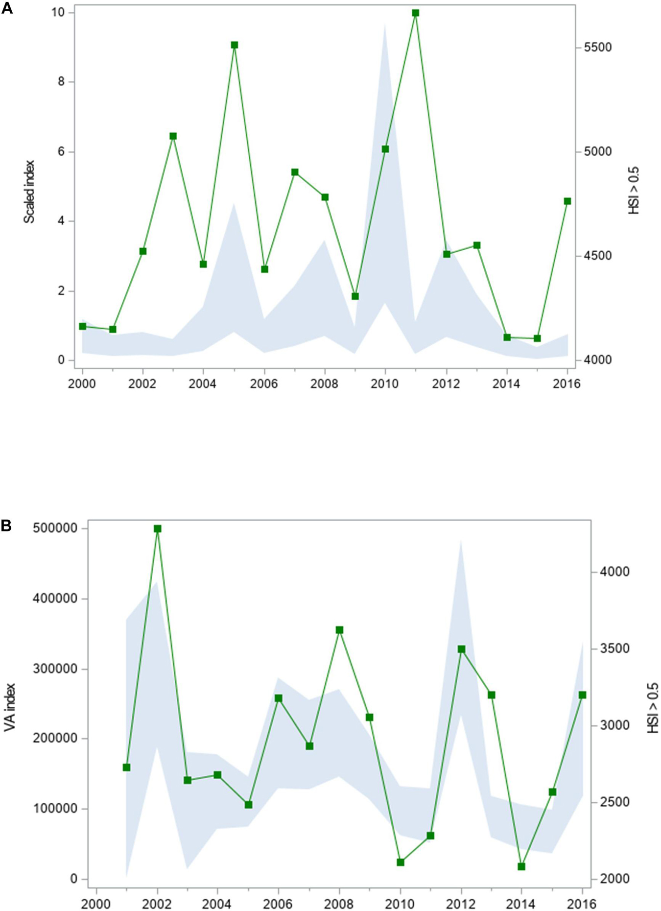
Figure 9. Relative abundance (scaled index) and extent of suitable habitat (km²) for (A) juvenile spot in summer and (B) bay anchovy in winter in Chesapeake Bay, 2000–2016. Relative abundance (solid polygon) is depicted with a 95% credible interval; area of suitable habitat is denoted by filled squares. Values of HSI_am ≥ 0.5 were considered suitable habitat.

More commonly, we were unable to detect a significant relationship between the area of suitable habitat and the rank-transformed estimate of baywide relative abundance of forage fishes (Tables 2, 3). For juvenile spotted hake in spring, we found no indication that the extent of suitable habitat was limiting, except perhaps in 2002 when the area of suitable habitat declined below 1,600 km² and the ranked abundance index was among the lowest observed in the time series. This, however, may be coincidental. The extent of suitable spring habitat for spotted hake varied without trend since 2000 (Tables 2, 3). We found no evidence of an effect of the extent of suitable habitat on the ranked relative abundance of juvenile spot in fall (Tables 2, 3). The extent of suitable habitat for juvenile spot in fall exhibited no trend through time (Tables 2, 3) and was markedly less than in summer. Between 2000 and 2016, the extent of suitable habitat for juvenile weakfish increased significantly in summer and fall (Tables 2, 3 and Figures 10A,B). The relative abundance of juvenile weakfish, however, exhibited no detectable response to increases in the extent of suitable habitats in either summer or fall during the study period (Tables 2, 3). Relative abundances of bay anchovy in spring and summer were highly variable (Figure 7) and annual estimates were imprecise. Although the extent of suitable spring and summer habitats for bay anchovy increased significantly since 2000 (Tables 2, 3 and Figures 10C,D), we did not detect a response in the ranked relative abundance of bay anchovy to changes in the extent of suitable habitats in spring or summer (Tables 2, 3).

FIGURE 10

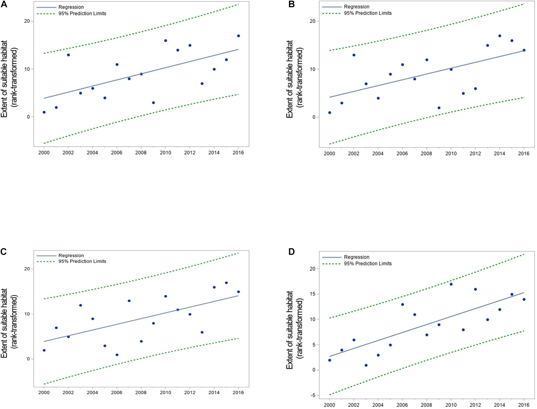
Figure 10. Pattern of change in the extent of suitable habitat for (A) juvenile weakfish in summer, (B) juvenile weakfish in fall, (C) bay anchovy in spring, and (D) bay anchovy in summer in Chesapeake Bay, 2000–2016. The extent of suitable habitat was rank-transformed due to the low sample size (n = 17), and the regression line estimates the nonparametric fit to the data. Regression slopes were positive and significantly different from 0 at the α = 0.05 level (Table 3). Values of HSI_am ≥ 0.5 were considered suitable habitat.

Discussion

Our modeling framework combined the power of machine learning to identify influential habitat covariates with the flexibility of non-parametric approaches to characterize habitat suitability and the capabilities of GIS to quantify and depict suitable (and unsuitable) habitats for forage fishes in Chesapeake Bay from 2000 to 2016. We coupled catch information from fishery surveys with static features of the environment and outputs from models of dynamic conditions to depict suitable habitats in Chesapeake Bay. In an ecosystem-based approach, these habitats may be targeted for protection (e.g., by limiting habitat alterations or other human activities that may incidentally kill or injure forage fishes) or restoration (e.g., by improving water quality conditions), thereby promoting production of sufficient forage for predators. Importantly, our modeling approach for building forage-fish habitat suitability models for the Chesapeake Bay was calibrated and verified, thereby allowing estimation of habitat suitability for tributaries and embayments in Chesapeake Bay that are not routinely sampled by fishery surveys (e.g., Mobjack Bay, Potomac River). Furthermore, our results allow resource managers to focus protective measures on critical habitat areas in Chesapeake Bay, for example, shallow areas near coastlines in spring and summer which persistently support suitable habitats for multiple forage species. Our finding that shallow areas near coastlines are important habitats for some forage species is consistent with the observed ontogenetic habitat shift of juvenile weakfish, which move from salt marsh tributaries to shallow habitats near coastlines in summer (Boutin and Targett, 2019). We found annual patterns in suitable habitat extent that mirrored those of baywide relative abundance for two of the species examined, juvenile spot in summer and bay anchovy in winter; as such, estimates of the minimum habitat area required to produce a desired abundance (or biomass) of forage fish can be used to establish quantitative habitat targets (Kritzer et al., 2016) or spatial thresholds that may serve as spatial reference points for management (Reuchlin-Hugenholtz et al., 2016). Quantitative habitat targets and spatial reference points for bay anchovy and juvenile spot in the Chesapeake Bay warrant further consideration.

Suitable seasonal habitat extents for forage species exhibited annual changes reflecting annual-scale heterogeneity in habitat conditions in Chesapeake Bay, with persistent seasonal signals that varied among species. Current speed, water depth, and either temperature or DO were important covariates for the four species we examined, and distance to shore was important for three species; thus, suitable habitat conditions resulted from a complex interplay between water quality and the geophysical properties of the habitat. Variations in seasonal extents were more pronounced than annual variations in suitable habitat extent, supporting the notion that the Chesapeake Bay serves as a nursery area for juvenile fishes and that the nursery function is temporally restricted and varies among species (e.g., spring for juvenile spotted hake, and summer for juvenile spot and weakfish). For some species, the extent of suitable seasonal habitat increased since 2000 (summer and fall habitats for juvenile weakfish, and spring and summer habitats for bay anchovy), whereas for other species, extents varied annually with no clear trend. None of the species examined were at the southern limit of their geographic range, and as waters of the Chesapeake Bay continue to warm (Hinson et al., 2021), we expect that suitable habitat extent may increase for species with broad thermal tolerances such as spot, weakfish, and bay anchovy. Other climate-related effects predicted for the region include increased precipitation and sea-level rise, both of which may alter salinity and salinity stratification. Salinity mediates the thermal tolerances of some fishes (e.g., Lankford and Targett, 1994; Nepal and Fabrizio, 2020) and could serve to limit suitable habitats in the future. When coupled with field observations, laboratory-based investigations of the interactive effects of salinity on the thermal tolerances for these forage species could be informative (e.g., Lankford and Targett, 1994).

The relationship between the extent of suitable habitat and relative abundance of forage species was species-dependent and when present, varied seasonally. Such relationships have not been widely explored for aquatic species. Although manipulative field experiments permit exploration of these relationships on small spatial scales (e.g., Parsons et al., 2014), only a few studies attempted to relate extent of suitable habitat and relative abundance of aquatic species using large-scale, field-based observations (e.g., Holbrook et al., 2000; Le Pape et al., 2003; Sundblad et al., 2014; French et al., 2018; Yu et al., 2019). For example, Yu et al. (2019) used a graphical assessment to note the consistency between declines in the relative abundance of neon flying squid Ommastrephes bartramii and the spatial shrinkage of suitable habitats in the northwest Pacific Ocean. Sundblad et al. (2014) used linear regression to examine relationships between relative adult abundance and the percent of the study area that was suitable nursery habitat for 12 populations of pikeperch Sander lucioperca and European perch Perca fluviatilis. Here, we used non-parametric regression to statistically evaluate the strength of such relationships for forage fishes in Chesapeake Bay during 17 years and found a positive relationship between suitable habitat extent and baywide relative abundance of juvenile spot in summer and bay anchovy in winter, indicating that environmental and geophysical conditions affect the carrying capacity of the Chesapeake Bay for these species during a portion of the year. As such, our results are consistent with the findings of a meta-analysis of the correlation between abundance and indicators of habitat suitability (Weber et al., 2017).

We found no evidence that suitable habitat extents were limiting in Chesapeake Bay for juvenile spotted hake in spring, juvenile spot in fall, juvenile weakfish in summer and fall, and bay anchovy in spring and summer. These results suggest that seasonal suitable habitat extent exceeded that necessary to support these populations, and that other factors such as predation mortality (e.g., Minello et al., 1989), food availability (e.g., Tableau et al., 2016), or degradation of egg and larval habitats (e.g., Sundblad et al., 2014) may have contributed to changes in relative abundances. For example, suitable habitat extent for juvenile weakfish in summer and fall increased significantly since 2000, but was not significantly related to changes in relative abundance of juvenile weakfish, suggesting that factors other than those considered in the suitability model exerted a greater role in driving annual fluctuations in abundance. Indeed, abundance and growth of juvenile weakfish are greatest in habitats that contain abundant mysid resources and that are found adjacent to large expanses of salt marsh (Boutin and Targett, 2019). Consideration of the spatial distribution and annual variation in mysid abundance may be required to further delineate suitable habitats for juvenile weakfish in Chesapeake Bay. Additionally, the lack of a significant relationship between annual relative abundance of juvenile weakfish and suitable habitat extent may have resulted from changes in predation mortality of juvenile weakfish. This hypothesis is consistent with the observed increase in natural mortality rates for this species in the 2000s (Atlantic States Marine Fisheries Commission [ASMFC], 2019; Krause et al., 2020); although the sources of increased natural mortality in weakfish remain unclear, increased predation is believed to have played a role (Atlantic States Marine Fisheries Commission [ASMFC], 2019). Abundances of other forage fishes may be limited by similar trophic interactions with their predators or prey, or by unsuitable egg and larval habitats in Chesapeake Bay.

Although habitat extents limited the relative abundance of juvenile spot in summer, no such limitation occurred in fall. We hypothesize that the summer-to-fall decoupling of the relationship between habitat extent and relative abundance of juvenile spot may be partly explained by temperature. Mean water temperatures in Chesapeake Bay are greatest in late August-early September and the increased metabolic rates and energy demands of predators during this time may increase predation mortality on juvenile spot. Rising water temperatures during this time may also affect the phenology of spot emigration resulting in earlier emigration and fewer juvenile spot remaining in the estuary during fall in warmer years. We were unable to detect a change in the extent of suitable fall habitats for juvenile spot between 2000 and 2016, but warming water temperatures in fall associated with directional climate change may alter future habitat conditions in fall for this species. Continued monitoring of fall abundances and a better understanding of the cues that trigger spot emigration in fall will be necessary to address this hypothesis.

Another possible reason for our inability to detect a relationship between suitable habitat area and baywide relative abundance of some forage fishes is that the suite of static and dynamic habitat covariates we considered failed to adequately describe suitable habitat conditions. For example, the abundance of predators, availability of prey, and proximity to biogenic habitats such as seagrass or oyster reefs may help to shape the distribution and abundance of forage fishes. In addition, seasonal relative abundance indices for many of the forage species were imprecise and hence were statistically invariable across time (based on 95% credible intervals of the baywide hierarchical index). Thus, a ‘good’ year with a relatively high mean index of abundance was not statistically discernible from a ‘poor’ year with a relatively low index; this lack of contrast may have hampered our ability to uncover a relationship between relative abundance indices and suitable habitat extents. These results suggest that if the abundance of forage fishes in Chesapeake Bay is changing, the temporal and spatial intensity of sampling by current fisheries surveys is insufficient to detect changes. Alternatively, and more likely, abundance may be stable but highly variable across years, as is typically exhibited by forage fishes (Hilborn et al., 2017). Continued monitoring will be critical to detect directional changes in abundance.

Seasonal variation in the geographic location of suitable estuarine habitats may be linked to variation in freshwater input (e.g., Rubec et al., 2019). In Chesapeake Bay, freshwater input influences salinity and salinity stratification; however, we identified additional hydrodynamic covariates such as temperature stratification and current speed that contributed to variation in suitable habitats. For example, for bay anchovy, the suitability of winter habitats was partly determined by bottom DO and the horizontal gradient in tidal-averaged current speeds. Water temperature was not considered in the HSI model for bay anchovy in winter, however, we cannot rule out temperature as an important covariate describing habitat conditions for bay anchovy in winter because bottom temperature and DO were correlated. Interestingly, the HSI model for juvenile spot also included bottom DO and a measure of temperature stratification, suggesting that multiple hydrodynamic factors are required to describe suitable habitats.

In this study, we considered information from two fishery-independent surveys, one of which yielded fewer annual observations but sampled shallow-water habitats across a large portion of the estuarine salinity gradient. Overall, our fisheries observations were collected at a relatively fine spatial resolution (>100 sites sampled/month) and high temporal intensity (monthly), thereby minimizing biases due to seasonal or short-term habitat use (e.g., by sampling only one or two months each year). By using fisheries observations from multiple surveys, we were able to detect the effect of bottom DO on the relative baywide abundance of juvenile spot in summer. Low bottom DO conditions in summer are more prevalent and persistent in Maryland waters of the Chesapeake Bay; in particular, the Chester River, Eastern Bay, Choptank River, Little Choptank River, and Patuxent River exhibited bottom DO levels in summer that were markedly lower than what was observed in Virginia waters. These observations extended the range of bottom DO conditions over which these effects could be investigated. In addition, the Maryland survey sampled sites in shallow habitats close to shore, and these conditions were not well sampled in Virginia waters. Together, the two surveys provided observations from a greater range of environmental and bathymetric conditions commonly encountered in the Chesapeake Bay region.

Hydrodynamic models and other numerical models of environmental conditions can provide information on dynamic habitat features that are not measured at the time of sampling and represent a significant advancement toward refining spatial relationships between fish and their environment (e.g., Crear et al., 2020a). Consideration of such information may yield habitat models with greater predictive accuracy (Scales et al., 2017). In our study, we used tidal-averaged conditions to develop habitat suitability models that reasonably reflected the relationship between (daily) environmental conditions and relative abundance (at the tow level) of forage fishes in Chesapeake Bay. This fine-scale approach is preferable to one that uses seasonal averages of habitat conditions to build habitat suitability models (Scales et al., 2017). Indeed, the temporal resolution of environmental covariates used to build the suitability model affects the scale of inference. For example, Woodland et al. (2021) described annual patterns in the distribution and abundance of forage fishes and invertebrates relative to patterns of predation and environmental conditions in the Chesapeake Bay and its major tributaries. Seasonal changes, however, could not be addressed because several habitat conditions were represented by annual means (e.g., average discharge from tributaries, and the Atlantic Multidecadal Oscillation [AMO] index). Large-scale climatic changes as indexed by the AMO affect mean abundances of bay anchovy and juvenile spot (Woodland et al., 2021), and our findings for bay anchovy in winter and juvenile spot in summer are consistent with findings in Woodland et al. (2021). Specifically, our results suggested that variations in environmental conditions contributed to the observed variation in relative abundance of these forage species. Although we did not consider large-scale climate indices per se, we did examine small-scale environmental indicators of climate change (temperature, salinity) and demonstrated how these changes affect habitat suitability and relative baywide indices of abundance for juvenile spot in summer and bay anchovy in winter. Unlike Woodland et al. (2021) who found greater relative abundance of bay anchovy in the upper bay than in the lower bay, our indices of relative abundance for bay anchovy in summer were an order of magnitude lower in Maryland than those observed in Virginia waters, likely because we lacked samples from deep sites (>2.7 m) in Maryland which were considered in Woodland et al. (2021). Also, the time scale of our studies differed. Similar to Woodland et al. (2021), we found that bay anchovy and juvenile spot exhibited higher relative abundances in southern tributaries than in northern tributaries of the Chesapeake Bay, but our spatial depiction of suitable habitat conditions throughout the system allowed us to examine the fine-scale spatial distribution of suitable habitats. Such depictions are helpful for identifying the geographic scale at which habitat protection or restoration must be implemented.

As the number of habitat descriptors available to researchers increases, variable reduction techniques are critical to the selection of covariates that help explain the variation in observed abundance and distribution of aquatic organisms. For example, satellite imagery, ocean observing systems, and hydrodynamic models yield a multitude of environmental descriptors of habitat and these data are commonly used to inform fish habitat models. Similar to Georgian et al. (2019), we used BRTs to identify influential covariates from a large suite of possible covariates. Because tree complexity can play a large role in improving the outcome of cross-validation and BRT model fitting, BRT parameters should be optimized using the data under consideration. Many researchers either fail to optimize regression trees or when optimization is implemented, only a single parameter is optimized (typically learning rate; e.g., Georgian et al., 2019; Yu et al., 2020) after using the default bag fraction (0.75) and selecting an arbitrary value for tree complexity (typically between 2 and 5; e.g., Georgian et al., 2019; Pennino et al., 2020; Yu et al., 2020). We recommend optimization of BRTs using the approach we applied here or the R package gbm.auto (Dedman et al., 2017).

Across the four species we examined, the geometric mean formulation of the HSI was best for only a single species – juvenile spotted hake. Although the HSI_gm is widely used, this formulation may penalize the index too harshly for mobile species that can tolerate broad variations in environmental conditions, including sub-optimal conditions for limited periods of time. For instance, in areas where bottom temperature exceeds a given species’ thermal tolerance, the SI for bottom temperature may be close to 0; in this case, the value of the HSI_gm will also be close to 0, but other environmental conditions in these areas may be suitable, even optimal, and thus, the overall suitability may not be well indexed by the HSI_gm. Because the appropriate HSI formulation depends on species, we recommend use of data-driven analyses and assessment of model performance to inform selection (Chang et al., 2012; Tanaka and Chen, 2015; Yu et al., 2019; this study).

Our fisheries observations from two surveys that sampled across a broad geographic area of the largest estuary in the United States represented 17 years of monthly sampling and reflected the breadth of habitat conditions that fishes were likely to encounter in Chesapeake Bay. Although survey designs differed (stratified random design in Virginia, and fixed-site design in Maryland), the integration of information from such surveys can provide models with good predictive performance as long as observations are spatially extensive (Soranno et al., 2020). Furthermore, when the number of observations used to fit the model is sufficiently large, then projections for unsampled areas within the same time frame are considered valid interpolations (Elith and Leathwick, 2009; Soranno et al., 2020). Our projections of HSIs in areas not sampled by the Maryland or Virginia surveys (e.g., Mobjack Bay, Potomac River) were based on 25,333 observations, and as such, were valid interpolations for assessment of habitat conditions in non-sampled areas during the timeframe of the study (2000–2016). Our interpolations did not ‘extend beyond the conditions represented by the data used to fit the model,’ and thus we avoided extrapolations to areas where novel combinations of predictors occur (Conn et al., 2015).

Finally, we note that the uncertainties associated with habitat suitability modeling and resulting projections are not typically assessed (Elith and Leathwick, 2009), although such uncertainties are useful for understanding the limitations of model-based results for conservation and fisheries management. Uncertainties may arise from model specification (e.g., the type of model used, or covariates omitted from the model) and from the observations used to fit the model (e.g., samples may not represent the population of interest, or sample size may be inadequate). Ensemble approaches have been used to partially mitigate model uncertainty, but ensemble models do not fully overcome the limitations of the individual component models (Elith et al., 2010). Model and observational uncertainties may affect habitat suitability projections in different ways, and uncertainty analysis for HSI models warrants further research (Zajac et al., 2015) and engagement with environmental statisticians.

Data Availability Statement

The data analyzed in this study are subject to the following licenses/restrictions: William & Mary ScholarWorks (https://scholarworks.wm.edu/) provides open public access to the monthly abiotic data collected as part of the VIMS trawl survey (https://doi.org/10.25773/97cg-7w42), the seasonal habitat suitability maps (https://doi.org/10.25773/d37g-1h89), and the estimated areas of suitable habitat (https://doi.org/10.25773/d37g-1h89) for 2000 to 2016. Maps and data are under a CC-NC-SA 4.0 license. Maryland trawl survey data should be requested from the original data source.

Author Contributions

All the authors conceptualized the research, performed the analyses, interpreted the results, read and approved the published version of the manuscript. MF prepared the original draft of the manuscript. TT, AB, and MM contributed to writing and editing of the manuscript. MF and AB contributed to the project administration and visualization. MF and TT contributed to the funding acquisition.

Funding

This study was funded by the NOAA Chesapeake Bay Office, grant NA17NMF4570156 to the authors.

Conflict of Interest

AB and MM are employed by Anchor QEA, LLC.

The remaining authors declare that the research was conducted in the absence of any commercial or financial relationships that could be construed as a potential conflict of interest.

Publisher’s Note

All claims expressed in this article are solely those of the authors and do not necessarily represent those of their affiliated organizations, or those of the publisher, the editors and the reviewers. Any product that may be evaluated in this article, or claim that may be made by its manufacturer, is not guaranteed or endorsed by the publisher.

Acknowledgments

The UnTRIM code used in the hydrodynamic modeling was developed and provided by Professor Vincenzo Casulli (University of Trento, Italy). We thank J. Shen (Virginia Institute of Marine Science, VIMS) and B. Marcek (US Fish & Wildlife Service) for extending the model of bottom DO conditions. We are grateful to J. Buchanan (VIMS) and V. Nepal (VIMS) for application and verification of the DO model, to W. Lowery (VIMS) for preparing Figure 1, and to R. Dixon (VIMS) and S. Smith (VIMS) for assistance with verification of the HSI modeling approach. We thank C. Walstrum (MD DNR) for providing fisheries data from the Maryland trawl survey. We appreciate the steadfast sampling in Virginia tidal waters by Captains H. Brooks, V. Hogge, and W. Lowery, and the scientific crew of the VIMS Juvenile Fish Trawl Survey that participated in trawl sampling between 2000 and 2016. Finally, we thank the reviewers for comments that helped to improve the manuscript. This manuscript is Contribution No. 4051 of the Virginia Institute of Marine Science, William & Mary.

Supplementary Material

The Supplementary Material for this article can be found online at: https://www.frontiersin.org/articles/10.3389/fmars.2021.706666/full#supplementary-material

References

Arbeider, M., Sharpe, C., Carr-Harris, C., and Moore, J. W. (2019). Integrating prey dynamics, diet, and biophysical factors across an estuary seascape for four fish species. Mari. Ecol. Progr. Ser. 613, 151–169. doi: 10.3354/meps12896

CrossRef Full Text | Google Scholar

Atlantic States Marine Fisheries Commission [ASMFC] (2018). Five-Year Strategic Plan 2019-2023. Available online at: http://www.asmfc.org/fisheries-management/program-overview (accessed September 23, 2021).

Google Scholar

Atlantic States Marine Fisheries Commission [ASMFC] (2019). Weakfish Stock Assessment Update Report. Available online at: http://asmfc.org/species/weakfish (accessed September 23, 2021).

Google Scholar

Bever, A. J., MacWilliams, M. L., Herbold, B., Brown, L. R., and Feyrer, F. V. (2016). Linking hydrodynamic complexity to delta smelt (Hypomesus transpacificus) distribution in San Francisco Estuary, USA. San Francisco Estuary Watershed Sci. 14, 1–27. doi: 10.15447/sfews.2016v14iss1art3

CrossRef Full Text | Google Scholar

Birkmanis, C. A., Freer, J. J., Simmons, L. W., Partridge, J. C., and Sequeira, A. M. M. (2020). Future distribution of suitable habitat for pelagic sharks in Australia under climate change models. Front. Mari. Sci. 7:570. doi: 10.3389/fmars.2020.00570

CrossRef Full Text | Google Scholar

Boutin, B. P., and Targett, T. E. (2019). Density, growth, production, and feeding dynamics of juvenile weakfish (Cynoscion regalis) in Delaware Bay and salt marsh tributaries: spatiotemporal comparison of nursery habitat quality. Estuaries Coasts 42, 274–291. doi: 10.1007/s12237-018-0457-9

CrossRef Full Text | Google Scholar

Brady, D. C., and Targett, T. E. (2013). Movement of juvenile weakfish Cynoscion regalis and spot Leiostomus xanthurus in relation to diel-cycling hypoxia in an estuarine tidal tributary. Mari. Ecol. Progr. Seri. 491, 199–219. doi: 10.3354/meps10466

CrossRef Full Text | Google Scholar

Breiman, L., Friedman, J. H., Olshen, R. A., and Stone, C. J. (1984). Classification and Regression Trees. New York: Chapman and Hall.

Google Scholar

Brown, S. K., Buja, K. R., Jury, S. H., and Monaco, M. E. (2000). Habitat suitability index models for eight fish and invertebrate species in Casco and Sheepscot Bays, Maine. North Am. J. Fish. Manag. 20, 408–435. doi: 10.1577/1548-8675(2000)020<0408:hsimfe>2.3.co;2

CrossRef Full Text | Google Scholar

Buchheister, A., Bonzek, C. F., Gartland, J., and Latour, R. J. (2013). Patterns and drivers of the demersal fish community of Chesapeake Bay. Mari. Ecol. Progr. Ser. 481, 161–180. doi: 10.3354/meps10253

CrossRef Full Text | Google Scholar

Buchheister, A., and Latour, R. J. (2011). Trophic ecology of summer flounder in lower Chesapeake Bay inferred from stomach content and stable isotope analyses. Trans. Am. Fish. Soc. 140, 1240–1254. doi: 10.1080/00028487.2011.618364

CrossRef Full Text | Google Scholar

Buchheister, A., and Latour, R. J. (2015). Diets and trophic-guild structure of a diverse fish assemblage in Chesapeake Bay, U.S.A. J. Fish Biol. 86, 967–992. doi: 10.1111/jfb.12621

PubMed Abstract | CrossRef Full Text | Google Scholar

Byrne, R. J., Hobbs, C. H. III, and Carron, M. J. (1983). Baseline Sediment Studies To Determine Distribution, Physical Properties, Sedimentation Budgets, And Rates in The Virginia Portion Of The Chesapeake Bay. Final Report To The US Environmental Protection Agency Chesapeake Bay Program. Gloucester Point, VA: Virginia Institute of Marine Science.

Google Scholar

Cameron, M. J., Lucieer, V., Barrett, N. S., Johnson, C. R., and Edgar, G. J. (2014). Understanding community-habitat associations of temperate reef fishes using fine-resolution bathymetric measures of physical structure. Mari. Ecol. Progr. Ser. 506, 213–229. doi: 10.3354/meps10788

CrossRef Full Text | Google Scholar

Casulli, V., and Zanolli, P. (2002). Semi-implicit numerical modelling of non-hydrostatic free-surface flows for environmental problems. Math. Comput. Mod. 36, 1131–1149. doi: 10.1016/s0895-7177(02)00264-9

CrossRef Full Text | Google Scholar

Casulli, V., and Zanolli, P. (2005). High-resolution methods for multidimensional advection-diffusion problems in free-surface hydrodynamics. Ocean Mod. 10, 137–151. doi: 10.1016/j.ocemod.2004.06.007

CrossRef Full Text | Google Scholar

Chang, Y.-J., Sun, C.-L., Chen, Y., Yeh, S.-Z., and Dinardo, G. (2012). Habitat suitability analysis and identification of potential fishing grounds for swordfish, Xiphias gladius, in the South Atlantic Ocean. Int. J. Remote Sensing 33, 7523–7541. doi: 10.1080/01431161.2012.685980

CrossRef Full Text | Google Scholar

Conn, P. B. (2010). Hierarchical analysis of multiple noisy abundance indices. Can. J. Fish. Aquatic Sci. 67, 108–120. doi: 10.1139/f09-175

PubMed Abstract | CrossRef Full Text | Google Scholar

Conn, P. B., Johnson, D. S., and Boveng, P. L. (2015). On extrapolating past the range of observed data when making statistical predictions in ecology. PLoS One 10:e0141416. doi: 10.1371/journal.pone.0141416

PubMed Abstract | CrossRef Full Text | Google Scholar

Craig, J. K., and Crowder, L. B. (2005). Hypoxia-induced habitat shifts and energetic consequences in Atlantic croaker and brown shrimp on the Gulf of Mexico shelf. Mari. Ecol. Progr. Ser. 294, 79–94. doi: 10.3354/meps294079

CrossRef Full Text | Google Scholar

Crear, D. P., Latour, R. J., Friedrichs, M. A. M., St-Laurent, P., and Weng, K. C. (2020a). Sensitivity of a shark nursery habitat to a changing climate. Mari. Ecol. Progr. Ser. 652, 123–136. doi: 10.3354/meps13483

CrossRef Full Text | Google Scholar

Crear, D. P., Watkins, B. E., Saba, V. S., Graves, J. E., Jensen, D. R., Hobday, A. J., et al. (2020b). Contemporary and future distributions of cobia, Rachycentron canadum. Biodiversity Res. 26, 1002–1015. doi: 10.1111/ddi.13079

CrossRef Full Text | Google Scholar

Day, J. W. Jr., Hall, C. A. S., Kemp, W. M., and Yáñez-Arancibia, A. (1989). Estuarine Ecology. New York: John Wiley & Sons.

Google Scholar

Dedman, S., Officer, R., Clarke, M., Reid, D. G., and Brophy, D. (2017). Gbm.auto: a software tool to simplify spatial modelling and marine protected area planning. PLoS One 12:e0188955. doi: 10.1371/journal.pone.0188955

PubMed Abstract | CrossRef Full Text | Google Scholar

Du, J., and Shen, J. (2014). Decoupling the influence of biological and physical processes on the dissolved oxygen in the Chesapeake Bay. J. Geophys. Res. Oceans 120, 78–93. doi: 10.1002/2014jc010422

CrossRef Full Text | Google Scholar

Efron, B., and Tibshirani, R. (1986). Bootstrap methods for standard errors, confidence intervals, and other measures of statistical accuracy. Statist. Sci. 1, 54–77.

Google Scholar

Elith, J., Kearney, M., and Phillips, S. (2010). The art of modelling range-shifting species. Methods Ecol. Evol. 1, 330–342. doi: 10.1111/j.2041-210x.2010.00036.x

CrossRef Full Text | Google Scholar

Elith, J., and Leathwick, J. (2017). Boosted Regression Trees For Ecological Modeling. Available online at: https://rspatial.org/raster/sdm/9_sdm_brt.html (accessed September 23, 2021).

Google Scholar

Elith, J., and Leathwick, J. R. (2009). Species distribution models: ecological explanation and prediction across space and time. Ann. Rev. Ecol. Evol. Syst. 40, 677–697. doi: 10.1146/annurev.ecolsys.110308.120159

CrossRef Full Text | Google Scholar

Elith, J., Leathwick, J. R., and Hastie, T. (2008). A working guide to boosted regression trees. J. Anim. Ecol. 77, 802–813. doi: 10.1111/j.1365-2656.2008.01390.x

PubMed Abstract | CrossRef Full Text | Google Scholar

Fabrizio, M. C., Manderson, J. P., and Pessutti, J. P. (2013). Habitat associations and dispersal of black sea bass from a mid-Atlantic Bight reef. Mari. Ecol. Progr. Ser. 482, 241–253. doi: 10.3354/meps10302

CrossRef Full Text | Google Scholar

França, S., Costa, M. J., and Cabral, H. N. (2009). Assessing habitat specific fish assemblages in estuaries along the Portuguese coast. Estuarine Coastal Shelf Sci. 83, 1–12. doi: 10.1016/j.ecss.2009.03.013

CrossRef Full Text | Google Scholar

Freitag, A., Vogt, B., and Hartley, T. (2018). Ecosystem-based fisheries management in the Chesapeake Bay: developing functional indicators. Coastal Manag. 46, 127–147. doi: 10.1080/08920753.2018.1451729

CrossRef Full Text | Google Scholar

French, K. J., Shackell, N. L., and den Heyer, C. E. (2018). Strong relationship between commercial catch of adult Atlantic halibut (Hippoglossus hippoglossus) and availability of suitable habitat for juveniles in the Northwest Atlantic Ocean. Fish. Bull. 116, 107–121.

Google Scholar

Fulford, R. S., Peterson, M. S., Wu, W., and Grammer, P. O. (2014). An ecological model of the habitat mosaic in estuarine nursery areas: part II – projecting effects of sea level rise on fish production. Ecol. Mod. 273, 96–108. doi: 10.1016/j.ecolmodel.2013.10.032

CrossRef Full Text | Google Scholar

Georgian, S. E., Anderson, O. F., and Rowden, A. A. (2019). Ensemble habitat suitability modeling of vulnerable marine ecosystem indicator taxa to inform deep-sea fisheries management in the South Pacific Ocean. Fish. Res. 211, 256–274. doi: 10.1016/j.fishres.2018.11.020

CrossRef Full Text | Google Scholar

Glaspie, C. N., Clouse, M., Huebert, K., Ludsin, S. A., Mason, D. M., Pierson, J. J., et al. (2019). Fish diet shifts associated with the northern Gulf of Mexico hypoxic zone. Estuaries Coasts 42, 2170–2183. doi: 10.1007/s12237-019-00626-x

CrossRef Full Text | Google Scholar

Gray, C. A., Rotherham, D., and Johnson, D. D. (2011). Consistency of temporal and habitat-related differences among assemblages of fish in coastal lagoons. Estuarine Coastal Shelf Sci. 95, 401–414. doi: 10.1016/j.ecss.2011.10.010

CrossRef Full Text | Google Scholar

Guan, L., Chen, Y., and Wilson, J. A. (2016). Evaluating spatio-temporal variability in the habitat quality of Atlantic cod (Gadus morhua) in the Gulf of Maine. Fish. Oceanogr. 26, 83–96. doi: 10.1111/fog.12188

CrossRef Full Text | Google Scholar

Hess, G. R., and Bay, J. M. (2000). A regional assessment of windbreak habitat suitability. Environ. Monit. Assess. 61, 237–254.

Google Scholar

Hilborn, R., Amoroso, R. O., Bogazzi, E., Jensen, O. P., Parma, A. M., Szuwalski, C., et al. (2017). When does fishing forage species affect their predators? Fishe. Res. 191, 211–221. doi: 10.1016/j.fishres.2017.01.008

CrossRef Full Text | Google Scholar

Hinson, K., Friedrichs, M. A. M., St-Laurent, P., Da, F., and Najjar, R. G. (2021). Extent and causes of Chesapeake Bay warming. J. Am. Water Res. Assoc. 1–21. doi: 10.1111/1752-1688.12916

CrossRef Full Text | Google Scholar

Holbrook, S. J., Forrester, G. E., and Schmitt, R. J. (2000). Spatial patterns in abundance of a damselfish reflect availability of suitable habitat. Oecologia 122, 109–120. doi: 10.1007/pl00008826

PubMed Abstract | CrossRef Full Text | Google Scholar

Irby, I. D., Friedrichs, M. A. M., Friedrichs, C. T., Bever, A. J., Hood, R. R., Lanerolle, L. W. J., et al. (2016). Challenges associated with modeling low-oxygen waters in Chesapeake Bay: a multiple model comparison. Biogeosciences 13, 2011–2028. doi: 10.5194/bg-13-2011-2016

CrossRef Full Text | Google Scholar

Jaonalison, H., Durand, J.-D., Mahafina, J., Demarcq, H., Teichert, N., and Ponton, D. (2020). Predicting species richness and abundance of tropical post-larval fish using machine learning. Mari. Ecol. Progr. Ser. 645, 125–139. doi: 10.3354/meps13385

CrossRef Full Text | Google Scholar

Jenkins, G. P., Spooner, D., Conron, S., and Morrongiello, J. R. (2015). Differing importance of salinity stratification and freshwater flow for the recruitment of apex species of estuarine fish. Mari. Ecol. Progr. Ser. 523, 125–144. doi: 10.3354/meps11147

CrossRef Full Text | Google Scholar

Kerhin, R. T., Halka, J. P., Wells, D. V., Hennessee, E. L., Blakeslee, P. J., Zoltan, N., et al. (1988). Chesapeake Bay Earth Science Study (CBESS): Physical Properties of Surficial Sediments, Chesapeake Bay, Maryland (Tabular Data). Baltimore, Maryland: Maryland Geological Survey. Available online at: http://www.mgs.md.gov/coastal_geology/baysedata.html (accessed September 23, 2021).

Google Scholar

Knudby, A., Brenning, A., and LeDrew, E. (2010). New approaches to modelling fish-habitat relationships. Ecol. Mod. 221, 503–511. doi: 10.1016/j.ecolmodel.2009.11.008

CrossRef Full Text | Google Scholar

Kostecki, C., Le Loc’h, F., Roussel, J.-M., Desroy, N., Huteau, D., Riera, P., et al. (2010). Dynamics of an estuarine nursery ground: the spatio-temporal relationship between the river flow and the food web of the juvenile common sole as revealed by stable isotope analysis. J. Sea Res. 64, 54–60. doi: 10.1016/j.seares.2009.07.006

CrossRef Full Text | Google Scholar

Krause, J. R., Hightower, J. E., Buckel, J. A., Turnure, J. T., Grothues, T. M., Manderson, J. P., et al. (2020). Using acoustic telemetry to estimate weakfish survival rates along the U.S. east coast. Mari. Coastal Fish. 12, 241–257. doi: 10.1002/mcf2.10095

CrossRef Full Text | Google Scholar

Kritzer, J. P., Delucia, M., Greene, E., Shumway, C., Topolski, M. F., Thomas-Blate, J., et al. (2016). The importance of benthic habitats for coastal fisheries. BioScience 66, 274–284.

Google Scholar

Lankford, T. E. Jr., and Targett, T. E. (1994). Suitability of estuarine nursery zones for juvenile weakfish (Cynoscion regalis): effects of temperature and salinity on feeding, growth and survival. Mari. Biol. 119, 611–620. doi: 10.1007/bf00354325

CrossRef Full Text | Google Scholar

Latour, R. J., Gartland, J., Bonzek, C. F., and Johnson, R. (2008). The trophic dynamics of summer flounder (Paralichthys dentatus) in Chesapeake Bay. Fish. Bull. 106, 47–57.

Google Scholar

Lauver, C. L., Busby, W. H., and Whistler, J. L. (2002). Testing a GIS model of habitat suitability for a declining grassland bird. Environ. Manag. 30, 88–97. doi: 10.1007/s00267-001-2609-z

PubMed Abstract | CrossRef Full Text | Google Scholar

Layher, W. G., and Maughan, O. E. (1985). Spotted bass habitat evaluation using an unweighted geometric mean to determine HSI values. Proc. Oklahoma Acad. Sci. 65, 11–17.

Google Scholar

Le Pape, O., Chauvet, F., Mahevas, S., Lazure, P., Guerault, D., and Desaunay, Y. (2003). Quantitative description of habitat suitability for the juvenile common sole in the Bay of Biscay (France) and the contribution of different habitats to the adult population. J. Sea Res. 50, 139–149. doi: 10.1016/s1385-1101(03)00059-5

CrossRef Full Text | Google Scholar

Lecours, V., Devillers, R., Schneider, D. C., Lucieer, V. L., Brown, C. J., and Edinger, E. N. (2015). Spatial scale and geographic context in benthic habitat mapping: review and future directions. Mari. Ecol. Progr. Ser. 535, 259–284. doi: 10.3354/meps11378

CrossRef Full Text | Google Scholar

Leslie, H. M. (2018). Value of ecosystem-based management. Proc. Natl. Acad. Sci. U.S.A. 115, 3518–3520.

Google Scholar

Little, A. G., Loughland, I., and Seebacher, F. (2020). What do warming waters mean for fish physiology and fisheries? J. Fish Biol. 97, 328–340. doi: 10.1111/jfb.14402

PubMed Abstract | CrossRef Full Text | Google Scholar

MacWilliams, M. L., Bever, A. J., and Foresman, E. (2016). 3-D simulations of the San Francisco Estuary with subgrid bathymetry to explore long-term trends in salinity distribution and fish abundance. San Francisco Estuary Watershed Sci. 14, 1–24.

Google Scholar

Manderson, J. P., Palamara, L., Kohut, J., and Oliver, M. J. (2011). Ocean observatory data are useful for regional habitat modeling of species with different vertical habitat preferences. Mari. Ecol. Progr. Ser. 438, 1–17. doi: 10.3354/meps09308

CrossRef Full Text | Google Scholar

Manderson, J. P., Pessutti, J., Hilbert, J. G., and Juanes, F. (2004). Shallow water predation risk for a juvenile flatfish (winter flounder; Pseudopleuronectes americanus, Walbaum) in a northwest Atlantic estuary. J. Exp. Mari. Biol. Ecol. 304, 137–157. doi: 10.1016/j.jembe.2003.12.004

CrossRef Full Text | Google Scholar

Maryland Geological Survey (1996). Baltimore Harbor Surficial Sediments: Texture and Chemistry Baltimore, Maryland (Tabular Data). Maryland Department of Natural Resources, Maryland Geological Survey. Available online at: http://www.mgs.md.gov/publications/data_pages/baltoharbdata.html (accessed September 23, 2021).

Google Scholar

Miller, P. J., Lubke, G. H., McArtor, D. B., and Bergeman, C. S. (2016). Finding structure in data using multivariate tree boosting. Psychol. Methods 21, 583–602. doi: 10.1037/met0000087

PubMed Abstract | CrossRef Full Text | Google Scholar

Minello, T. J., Zimmerman, R. J., and Martinez, E. X. (1989). Mortality of young brown shrimp Penaeus aztecus in estuarine nurseries. Trans. Am. Fish. Soc. 118, 693–708. doi: 10.1577/1548-8659(1989)118<0693:moybsp>2.3.co;2

CrossRef Full Text | Google Scholar

Moncure, R., and Nichols, M. (1968). Characteristics of Sediments in the James River Estuary, Virginia. Special Scientific Report No. 53.

Google Scholar

Nepal, V., and Fabrizio, M. C. (2020). Sublethal effects of salinity and temperature on non-native blue catfish: Implications for establishment in Atlantic slope drainages. PLoS One 15:e0244392. doi: 10.1371/journal.pone.0244392

PubMed Abstract | CrossRef Full Text | Google Scholar

Overton, A. S., Manooch, C. S. III, Smith, J. W., and Brennan, K. (2008). Interactions between adult migratory striped bass (Morone saxatilis) and their prey during winter off the Virginia and North Carolina Atlantic coast from 1994 - 2007. Fish. Bull. 106, 174–182.

Google Scholar

Parsons, D. M., Middleton, C., Smith, M. D., and Cole, R. G. (2014). The influence of habitat availability on juvenile fish abundance in a northeastern New Zealand estuary. New Zealand J. Mari. Fresh. Res. 48, 216–228. doi: 10.1080/00288330.2013.875927

CrossRef Full Text | Google Scholar

Pennino, M. G., Coll, M., Albo-Puigserver, M., Fernández-Corredor, E., Steenbeek, J., Giráldez, A., et al. (2020). Current and future influence of environmental factors on small pelagic fish distributions in the northwestern Mediterranean Sea. Front. Mari. Sci. 7:article622. doi: 10.3389/fmars.2020.00622

CrossRef Full Text | Google Scholar

R Core Team (2019). R: A Language and Environment for Statistical Computing. Vienna: R Foundation for Statistical Computing.

Google Scholar

Reid, J. M., Reid, J. A., Jenkins, C. J., Hastings, M. E., Williams, S. J., and Poppe, L. J. (2005). usSEABED: Atlantic Coast Offshore Surficial Sediment Data Release: U.S. Geological Survey Data Series 118, version 1.0.

Google Scholar

Reuchlin-Hugenholtz, E., Shackell, N. L., and Hutchings, J. A. (2016). Spatial reference points for groundfish. ICES J. Mari. Sci. 73, 2468–2478. doi: 10.1093/icesjms/fsw123

CrossRef Full Text | Google Scholar

Rubec, P. J., Santi, C., Ghile, Y., and Chen, X. (2019). Modeling and mapping to assess spatial distributions and population numbers of fish and invertebrate species in the lower Peace River and Charlotte Harbor, Florida. Mari. Coastal Fish. 11, 328–350. doi: 10.1002/mcf2.10086

CrossRef Full Text | Google Scholar

Scales, K. L., Hazen, E. L., Jacox, M. G., Edwards, C. A., Boustany, A. M., Oliver, M. J., et al. (2017). Scale of inference: on the sensitivity of habitat models for wide ranging marine predators to the resolution of environmental data. Ecography 40, 210–220. doi: 10.1111/ecog.02272

CrossRef Full Text | Google Scholar

Scharf, F. S., Manderson, J. P., Fabrizio, M. C., Pessutti, J. P., Rosendale, J. E., Chant, R. J., et al. (2004). Seasonal and interannual patterns of distribution and diet of bluefish within a middle Atlantic Bight estuary in relation to abiotic and biotic factors. Estuaries 27, 426–436. doi: 10.1007/bf02803535

CrossRef Full Text | Google Scholar

Schielzeth, H. (2010). Simple means to improve the interpretability of regression coefficients. Methods Ecol. Evol. 1, 103–113. doi: 10.1111/j.2041-210x.2010.00012.x

CrossRef Full Text | Google Scholar

Schlenger, A. J., North, E. W., Schlag, Z., Li, Y., Secor, D. H., Smith, K. A., et al. (2013). Modeling the influence of hypoxia on the potential habitat of Atlantic sturgeon: a comparison of two methods. Mari. Ecol. Progr. Ser. 483, 257–272. doi: 10.3354/meps10248

CrossRef Full Text | Google Scholar

Skern-Mauritzen, M., Ottersen, G., Handegard, N. O., Huse, G., Dingsør, G. E., Stenseth, N. C., et al. (2016). Ecosystem processes are rarely included in tactical fisheries management. Fish Fish. 17, 165–175. doi: 10.1111/faf.12111

CrossRef Full Text | Google Scholar

Soranno, P. A., Cheruvelil, K. S., Liu, B., Wang, Q., Tan, P.-N., Zhou, J., et al. (2020). Ecological prediction at macroscales using big data: does sampling design matter? Ecol. Appl. 30:e02123. doi: 10.1002/eap.2123

PubMed Abstract | CrossRef Full Text | Google Scholar

Sundblad, G., Bergström, U., Sandström, A., and Eklöv, P. (2014). Nursery habitat availability limits adult stock sizes of predatory coastal fish. ICES J. Mari. Sci. 71, 672–680. doi: 10.1093/icesjms/fst056

CrossRef Full Text | Google Scholar

Tableau, A., Brind’Amour, A., Woillez, M., and Le Bris, H. (2016). Influence of food availability on the spatial distribution of juvenile fish within soft sediment nursery habitats. J. Sea Res. 111, 76–87. doi: 10.1016/j.seares.2015.12.004

CrossRef Full Text | Google Scholar

Tanaka, K., and Chen, Y. (2015). Spatiotemporal variability of suitable habitat for American lobster in Long Island Sound. J. Shellfish Res. 34, 531–543. doi: 10.2983/035.034.0238

CrossRef Full Text | Google Scholar

Theuerkauf, S. J., and Lipcius, R. N. (2016). Quantitative validation of a habitat suitability index for oyster restoration. Front. Mari. Sci. 3:64. doi: 10.3389/fmars.2016.00064

CrossRef Full Text | Google Scholar

Tian, S., Chen, X., Chen, Y., Xu, L., and Dai, X. (2009). Evaluating habitat suitability indices derived from CPUE and fishing effort data for Ommatrephes bratramii in the northwestern Pacific Ocean. Fish. Res. 95, 181–188. doi: 10.1016/j.fishres.2008.08.012

CrossRef Full Text | Google Scholar

Tuckey, T. D., and Fabrizio, M. C. (2016). Variability in fish tissue proximate composition is consistent with indirect effects of hypoxia in Chesapeake Bay tributaries. Mari. Coastal Fish. 8, 1–15. doi: 10.1080/19425120.2015.1103824

CrossRef Full Text | Google Scholar

Tuckey, T. D., and Fabrizio, M. C. (2020). Estimating Relative Juvenile Abundance of Ecologically Important Finfish in the Virginia Portion of Chesapeake Bay. Final Report Submitted to Virginia Marine Resources Commission. Gloucester Point, VI: Virginia Institute of Marine Science, William & Mary.

Google Scholar

Tyler, R. M., and Targett, T. E. (2007). Juvenile weakfish Cynoscion regalis distribution in relation to diel-cycling dissolved oxygen in an estuarine tributary. Mari. Ecol. Progr. Ser. 333, 257–269. doi: 10.3354/meps333257

CrossRef Full Text | Google Scholar

Velinsky, D., Wade, T. L., Schlekat, C. E., McGee, B. L., and Presley, B. J. (1994). Tidal river sediments in the Washington DC area I. Distribution and sources of trace metals. Estuaries 17, 305–320. doi: 10.2307/1352665

CrossRef Full Text | Google Scholar

Weber, M. M., Stevens, R. D., Diniz-Filho, J. A. F., and Grelle, C. E. V. (2017). Is there a correlation between abundance and environmental suitability derived from ecological niche modelling? Meta Anal. Ecogr. 40, 817–828. doi: 10.1111/ecog.02125

CrossRef Full Text | Google Scholar

Windle, M. J. S., Rose, G. A., Devillers, R., and Fortin, M.-J. (2012). Spatio-temporal variations in invertebrate-cod-environment relationships on the Newfoundland–Labrador Shelf, 1995-2009. Mari. Ecol. Progr. Ser. 469, 263–278. doi: 10.3354/meps10026

CrossRef Full Text | Google Scholar

Woodland, R., Buchheister, A., Latour, R. J., Lozano, C., Houde, E., Sweetman, C. J., et al. (2021). Environmental drivers of forage fishes and benthic invertebrates at multiple spatial scales in a large temperate estuary. Estuaries Coasts 44, 921–938. doi: 10.1007/s12237-020-00835-9

CrossRef Full Text | Google Scholar

Yu, H., Cooper, A. R., and Infante, D. M. (2020). Improving species distribution model predictive accuracy using species abundance: application with boosted regression trees. Ecol. Mod. 432:109202. doi: 10.1016/j.ecolmodel.2020.109202

CrossRef Full Text | Google Scholar

Yu, W., Chen, X., Zhang, Y., and Yi, Q. (2019). Habitat suitability modelling revealing environmental-driven abundance variability and geographical distribution shift of winter-spring cohort of neon flying squid Ommastrephes bartramii in the northwest Pacific Ocean. ICES J. Mari. Sci. 76, 1722–1735. doi: 10.1093/icesjms/fsz051

CrossRef Full Text | Google Scholar

Zajac, Z., Stith, B., Bowling, A. C., Lantimm, C. A., and Swain, E. D. (2015). Evaluation of habitat suitability index models by global sensitivity and uncertainty analyses: a case study for submerged aquatic vegetation. Ecol. Evol. 5, 2503–2517. doi: 10.1002/ece3.1520

PubMed Abstract | CrossRef Full Text | Google Scholar

Zeng, X., Tanaka, K. R., Chen, Y., Wang, K., and Zhang, S. (2018). Gillnet data enhance performance of rockfishes habitat suitability index model derived from bottom-trawl survey data: a case study with Sebasticus marmoratus. Fish. Res. 204, 189–196. doi: 10.1016/j.fishres.2018.02.009

CrossRef Full Text | Google Scholar

Zhang, H., Ludsin, S. A., Mason, D. M., Adamack, A. T., Brandt, S. B., Zhang, X., et al. (2009). Hypoxia-driven changes in the behavior and spatial distribution of pelagic fish and mesozooplankton in the northern Gulf of Mexico. J. Exp. Mari. Biol. Ecol. 381, S80–S91.

Google Scholar