Analysis of 23 Years of Daily Cloud-Free Chlorophyll and Suspended Particulate Matter in the Greater North Sea

Keypoints

- Analysis of 23 years (1998–2020) of daily satellite-based chlorophyll and suspended particulate matter products in the Greater North Sea using DINEOF (Data Interpolating Empirical Orthogonal Functions).

- Description of changes in spring bloom phenology, with earlier blooms observed through time.

- The number of satellites used to obtain the data has an influence on retained variance, with at least 3 satellites needed for a correct representation of variability.

1. Introduction

The North Sea is a semi-enclosed shallow shelf sea in northwestern Europe, and it is one of the most productive seas in the world (Ducrotoy et al., 2000). It is surrounded by heavily populated countries with important industrial and agricultural activities, resulting in large quantities of nutrients and pollutants being added to the North Sea through riverine inputs (Ducrotoy et al., 2000). As a result, the North Sea has suffered from eutrophication issues during several decades (e.g., Desmit et al., 2020; Xu et al., 2020; Friedland et al., 2021). Despite de-eutrophication policies implemented since the 1990s, such as the EU Marine Strategy Framework Directive (MSFD) which aims at reaching a Good Environmental Status (GES) in European waters, the North Sea still receives relatively high nutrient inputs (nitrogen and phosphorous, Van der Zande et al., 2019b). This results in intense phytoplankton blooms occurring every year between March and October, with the southern parts of the North Sea, shallower and more affected by industrial and agricultural activities, presenting more intense blooms (Lancelot et al., 2005; Rousseau et al., 2013; Desmit et al., 2015, 2020). Phytoplankton blooms are at the basis of the marine food web, driving biogeochemical cycles, producing oxygen and acting as a carbon pump (Xu et al., 2020). Phytoplankton spatial and temporal dynamics can be influenced by several factors, including the availability of nutrients and light, water temperature, and grazing (Capuzzo et al., 2017; Xu et al., 2020).

Spring bloom onset in the open ocean typically occurs when turbulent mixing decays, causing convection to stop (Ferrari et al., 2015). On well-mixed environments, spring bloom onsets typically when the upper mixed layer is shallower than a given critical depth (Huisman et al., 1999). Some studies point out to a shift in the timing of the spring bloom in the North Sea to earlier dates in recent years (e.g., Desmit et al., 2020). While the causes for this are not completely understood, Hunter-Cevera et al. (2016) point to temperature-induced changes in phytoplankton cell-division rates as a possible cause. Increasing temperature trends observed in the North Sea (Høyer and Karagali, 2016) can therefore contribute to earlier phytoplankton blooms. Chlorophyll concentration (CHL) is used as a proxy for phytoplankton concentration, and Suspended Particulate Matter (SPM) is directly related to the amount of light that is available for primary producers (Capuzzo et al., 2015). Ocean color properties have been routinely measured from satellite for several decades (e.g., Sathyendranath et al., 2019), which allows for long-term studies. In order to assess the changes that have occurred in CHL and SPM in the North Sea, long-time series of daily data must be used (Philippart et al., 2010). Considering different hydrodynamic regions can also help understand how physical properties like currents and stratification influence the distribution of CHL and SPM (Capuzzo et al., 2017).

Interannual changes in CHL and SPM have been studied in the North Sea by several authors (e.g., Fettweis et al., 2007, 2014; Philippart et al., 2010; Capuzzo et al., 2015; Desmit et al., 2020) using in situ and/or satellite data. In situ data are sparse and long term series are very difficult to maintain. On the other hand, satellite data are affected by the presence of clouds or quality flagging (e.g., low sun angle in higher latitudes) that limit the amount of measurements. Gap-free estimates are needed when assessing long-term changes in the total concentration of CHL and SPM in coastal waters, for example in support of the MSFD in European waters. CHL time series are therefore used as an indicator for eutrophication (Ferreira et al., 2011), and satellite-derived gap-free CHL offer the temporal and spatial coverage necessary for such monitoring activities (Van der Zande et al., 2019b).

DINEOF (Data Interpolating Empirical Orthogonal Functions, Beckers and Rixen, 2003; Alvera-Azcárate et al., 2005) is an EOF-based technique that is used to interpolate missing data (due, for example, to the presence of clouds) in satellite data sets. It has been used in numerous works, with ocean color variables (e.g., Sirjacobs et al., 2011; Alvera-Azcárate et al., 2015), sea surface temperature (Alvera-Azcárate et al., 2005) or sea surface salinity (Alvera-Azcárate et al., 2015) among others and has shown to be reliable even with high amounts of missing data (e.g., Alvera-Azcárate et al., 2005, 2009).

The main objective of this work is to assess the spatial and temporal dynamics of CHL and SPM of the Greater North Sea over a period of 23 years (1998 to 2020) using a gap-free high spatial (1 km) and temporal (daily) satellite dataset. This analysis covers a wide area and the gap-free analysis allows for a better estimation of changes in CHL and SPM both in time and space. The spatial and temporal variability of these reconstructed variables will be assessed, with special attention to the timing of the spring bloom and how it has changed over the period of study. The dataset is composed of a varying number of satellite sensors, providing us with insight on the influence of the number of available satellites in the variability retained in the final product. Section 2 describes the satellite data used, the domain of study, and the reconstruction approach using DINEOF. Section 3 contains a brief description of the reconstruction results and the EOF basis obtained. Section 4 discusses the timing of the spring bloom onset and how it has changed over the considered period. Conclusions are provided in section 5.

2. Materials and Methods

2.1. Study Area

The domain of study is shown in Figure 1, and covers the North Sea and the easternmost part of the North Atlantic Ocean, from 48°N to 66°N and from 8°W to 12°E. The bathymetry in this region is very varied, from the shallow plains of the southern part of the North Sea, with depths of less than 50 m, to depths of more than 3,000 m north of the Faroe Islands. Within the shallow parts of the North Sea, the Norwegian channel surrounding Norway reaches up to 700 m. In the center of the North Sea, the Dogger bank is a shallow sandbank that extends over several tens of kilometers and is a productive fishing ground (e.g., Kröncke, 2011).

FIGURE 1

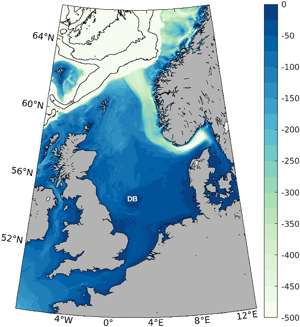
Figure 1. Domain of study with bathymetry (in m). The contours in the northwest part of the domain correspond to the 1,000, 2,000, and 3,000 m depth. DB shows the location of the Dogger Bank.

Circulation in the North Sea is mainly cyclonic, under the influence of prevailing westerly winds (Winther and Johannessen, 2006; Sündermann and Pohlmann, 2011). The main water inflow pathways are located at the northern part of the domain between the British Isles (mainly Shetland) and Norway, and in a lesser degree through the English Channel. Water also flows directly from the Atlantic Ocean toward the Baltic Sea through the Norwegian Channel. Tides are mainly semi-diurnal and follow also a cyclonic path in the North Sea (Sündermann and Pohlmann, 2011; Vindenes et al., 2018). The strong tidal currents result in strong mixing, specially in the shallower parts of the southern North Sea (Sündermann and Pohlmann, 2011).

2.2. Satellite Data

Generating reliable satellite estimates of CHL in optically complex coastal waters is still challenging. Many algorithms exist and give quite different performances for different optical conditions. For this reason, we applied the approach of Lavigne et al. (2021) who defined the limits of applicability of three popular and complementary algorithms: (1) the OC4 blue-green band ratio algorithm (O'Reilly et al., 1998) which was designed for open ocean waters; (2) the OC5 algorithm (Gohin et al., 2002) which is based on look-up tables and corrects OC4 overestimation in moderately turbid waters; and (3) a near infrared-red (NIR-red) band ratio algorithm (Gons et al., 2002) designed for high turbid waters. This approach allows automatic pixel-based switching between the most appropriate algorithms for a certain water type. Additionally, the neural-net approach FUB-WEW (Free University of Berlin Water processor, Fub v4.01, Schroeder et al., 2007) was used for the Kattegat region due to its high color dissolved organic matter concentration. Source products were obtained from publicly accessible archives: the Copernicus Marine Environment Monitoring Service (CMEMS), European Space Agency (i.e., ODESA) and other data providers (i.e., IFREMER). More details can be found in Van der Zande et al. (2019b). The SPM products were generated by applying the approach of Nechad et al. (2010) to the OC-CCI Remote Sensing Reflectance (Rrs) product obtained from CMEMS (OCEANCOLOUR_ATL_OPTICS_L3_REP_OBSERVATIONS _009_066, CMEMS data portal). All daily satellite products were generated with a spatial resolution of approximately 1 km, resulting in a matrix of 1913 × 1639 pixels in space for each day. The winter months December and January were excluded from the analysis as no ocean color products were available over a large part of the Greater North Sea due to low sun angle which complicates atmospheric correction procedures.

2.3. DINEOF

The CHL and SPM datasets were reconstructed using DINEOF (Data Interpolating Empirical Orthogonal Functions, Beckers and Rixen, 2003; Alvera-Azcárate et al., 2005). DINEOF calculates the expected value for the missing data based on the spatio-temporal information contained in the dataset, using a series of EOF modes. EOFs provide an efficient way of calculating the main modes of variability of a dataset, in order of increasing explained variance (von Storch and Zwiers, 1999). However, EOFs should not be directly calculated on uncomplete data, and DINEOF provides a way to overcome this and provide an estimate for the missing data at the same time. DINEOF calculates an EOF basis from the initial gappy data, by initiating the missing data to the average value of the matrix as first guess. As the matrix is demeaned to work with anomalies for the EOF decomposition, the initial missing data are in fact initialized with a value of zero. Using this matrix with zero at the missing locations, the first EOF (i.e., the main mode) is calculated. The missing data values are then recalculated using the EOF basis, obtaining an improved guess for those values. The process is iterated until convergence is reached for the missing data values. The number of EOF modes is increased (first one EOF, then the two first EOFs, and so on). Normally there can be as many EOF modes as the temporal size of the matrix being reconstructed (considering time as the smallest dimension, which is typically the case in satellite datasets). However, higher order EOFs contain a very small fraction of the total variability and may contain also noise and other transient errors, so in order to avoid retaining that information in the final product and to keep the computing time reasonable, only a truncated EOF series is used. The optimal number of EOFs that are retained for the final reconstruction of the missing data is determined by cross-validation: about 2-3% of valid data (i.e., not missing) are marked as missing data, and at each step DINEOF calculates the error between the initial data and the expected value provided by the EOF basis. The cross-validation data are taken in the form of clouds (as explained in Beckers et al., 2006) to better represent the nature of missing data in satellite images. DINEOF has been used in many previous works, and can be applied to variables like sea surface temperature and winds (Alvera-Azcárate et al., 2007), sea surface salinity (Alvera-Azcárate et al., 2016), chlorophyll (Huynh et al., 2020), etc.

Images with more than 98% of missing data were removed prior to the DINEOF reconstruction, which effectively removes mostly data from December and January. After removal of these images, there is still a very high amount of missing data, specially at high latitudes. As an example, the percentage of missing data for years 1998 and 2018 is shown in Figure 2. The percentage of missing data in 2018 is lower than in 1998 because of the availability of more satellite systems and sensors in recent years, namely MODIS, VIIRS and Sentinel-3 for recent years compared to only SeaWiFS in 1998 to 2002. The temporal distribution of the percentage of missing data (panel a of Figure 2) shows lower amounts of missing data during summer months, although on average there is always at least 60% of the domain with no data. Such a high amount of missing data makes it impractical to quantify the inter-annual variability with high confidence, and therefore an interpolation to reconstruct these gaps is necessary.

FIGURE 2

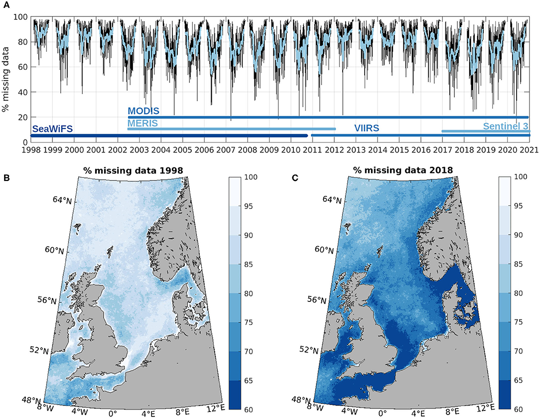
Figure 2. Percentage of missing data in the domain of study. (A) Spatially averaged percentage of missing data in the initial time series (black) and with a 30-day Gaussian low-pass filter (blue). (B) Temporal average of the percentage of missing data for 1998 (year with the highest average percentage of missing data). (C) Temporal average of the percentage of missing data for 2018 (year with the lowest average percentage of missing data).

Given the large size of the domain and the long time series that is being used in this work, each year has been reconstructed separately. Because December and January are not included in the analysis due to their high percentage of missing data, there is no continuity problem between each year. Making a separate analysis for each year also ensures that the EOF basis used for the reconstruction is not dominated by the main seasonal cycle. The data are transformed using a natural logarithm before the DINEOF analysis to ensure a distribution closer to a normal one.

2.4. Determination of Spring Bloom Onset Date

In order to assess the timing of the spring bloom in the North Sea and if this timing has changed through the years, we have used a threshold method following (Brody et al., 2013). The median of the North Sea CHL concentration is determined for every year and the date on which the concentration of CHL first reaches a value 5% above this median is chosen as the date the spring bloom starts. Other suggested methods in Brody et al. (2013), like the maximum rate of change in CHL growth, reflect the moment in which the bloom is already well underway and not in its starting phase. A 30-day Gaussian filtered time series is used to avoid short-term variations influencing in the calculation of the spring bloom timing.

3. DINEOF Results

In this section the main results obtained with DINEOF are presented. The reconstruction for each year has a different number of optimal EOFs depending on factors like the available data, the cloud coverage and the structures that are observed in the initial data (i.e., when no clouds or other missing data obscure them). For example, in the reconstruction of the CHL dataset in 1998 (the year with the maximum percentage of missing data), 5 EOFs were found optimal to reconstruct the missing data by DINEOF. For 2004, with a low percentage of missing data, 13 EOFs were found as optimal by DINEOF. For the SPM reconstructions, the minimum number of EOFs retained was 5 (for 2008) and the maximum was 19 (for 2009).

3.1. Validation

The multi-year dataset (both the original cloudy data and the DINEOF reconstruction) have been used in the frame of the EU-funded JMP-EUNOSAT project (Joint Monitoring Programme of the Eutrophication of the North Sea with Satellite data), to assess the use of satellite data to monitor the eutrophication in the North Sea with the help of satellite data, and a thorough validation has been realized in that project (Van der Zande et al., 2019a). The quality of the DINEOF reconstruction has been therefore assessed in the frame of the JMP-EUNOSAT project. The satellite-based CHL observations were compared to in situ observations collected in national monitoring programs. Differences between in situ and satellite CHL observations were quantified based on direct match ups within the in situ data archive. Considering all available data, the uncertainty is estimated with the Mean Absolute Difference (MAD) resulting in a value of 1.89 μg/l, which corresponds to a Mean Absolute Percentage Difference (MAPD) of 45.26%. The satellite products tend to overestimate CHL values when CHL is less than 1μg/l resulting in a slope of 0.64 and a relative high scatter (r² = 0.60) around the 1:1 line for higher CHL values. Validation of the DINEOF gap-filled products was performed with daily match up study using Dutch monitoring data ranging from clear to very turbid water conditions. Dutch monitoring data consisted of ship-based water samples collected between 1998 and 2016 in the Dutch coastal zone available at https://waterinfo.rws.nl/. Only surface samples (maximum depth of 3 m) analyzed using the HPLC method were accepted. The match-up analysis between the daily satellite CHL products and available in-situ CHL observations was performed following the approach of Bailey and Werdell (2006) allowing a maximum time difference of 2 hours. Applying the DINEOF technique results in a significant increase of available match ups (from 216 to 755) without strongly changing the correlation statistics (MAD original: 2.47 μg/l; MAD DINEOF: 2.83 μg/l, Figure 3) showing the potential of this approach to improve satellite-based observations for regions where satellite data availability is limited.

FIGURE 3

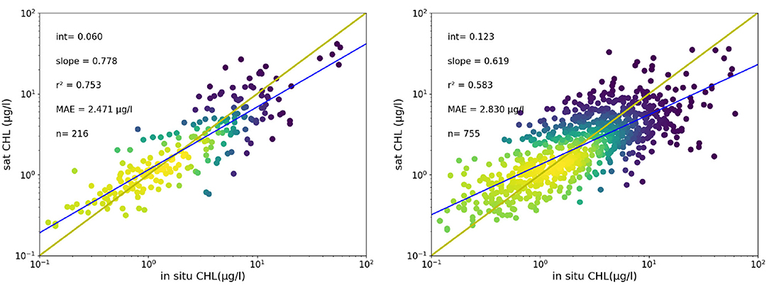
Figure 3. Scatterplots of in situ and satellite CHL observations for the Netherlands using the JMP-EUNOSAT CHL archive, without (left) and with DINEOF interpolation (right). The relationship between both data sets are described by the Mean Absolute Difference (MAD), Mean Absolute Percentage Error (MAPD). The determination coefficient (r²) and the slope characterizes the regression (adapted from Van der Zande et al., 2019b).

3.2. Example of Short-Term and Small-Scale Variability

An example of the reconstructed CHL data is shown in Figure 4, with a sequence of 5 days in May 2018 (with 5-day intervals to avoid showing too similar images). This sequence has been chosen because a CHL bloom is happening in the northernmost part of the domain, and the currents have advected the CHL which serves as a tracer for mesoscale eddies. These eddies are partially visible in the initial data, and the reconstruction is able to retain that kind of variability, even in a part of the domain that has a very large amount of missing data. In the central part of the North Sea, between Scotland and Norway, an elongated bloom is seen, which fades with time. This feature is also retained in the DINEOF reconstruction. Only one every 5 days is shown in Figure 4 for clarity, but intermediate dates also contributed to the final reconstruction and the shaping of the meso- and small-scale variability.

FIGURE 4

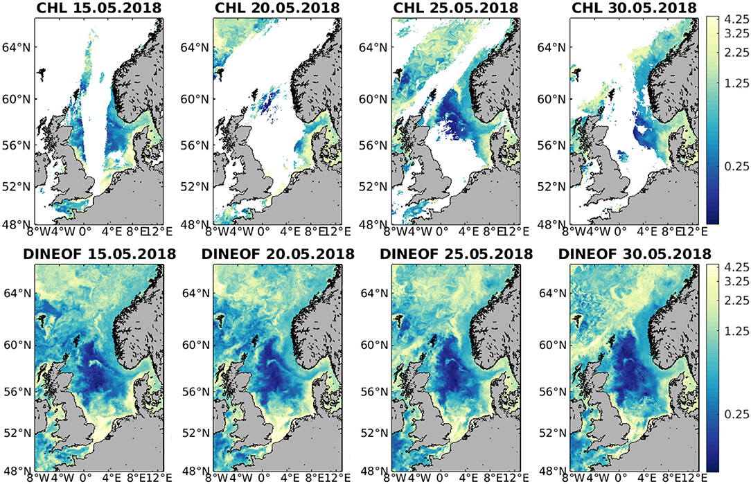
Figure 4. Example of CHL (μg/l) on 15, 20, 25, and 30 May 2018 for the initial data (top) and corresponding DINEOF reconstruction (bottom).

The same dates are also shown for SPM in Figure 5. Large SPM concentrations are found in the shallower regions in the southern half of the domain, which seem to decrease with time. The variability in the northern part of the domain is not as clearly observed in the initial SPM but the reconstruction seems to retain these scales as well. A high SPM concentration feature develops south of the Faroe Islands and in general we can appreciate that the concentration of SPM increases in the northern part of the domain during these days. The spatial and temporal variability retained by the DINEOF reconstruction is similar to what is observed in the initial data.

FIGURE 5

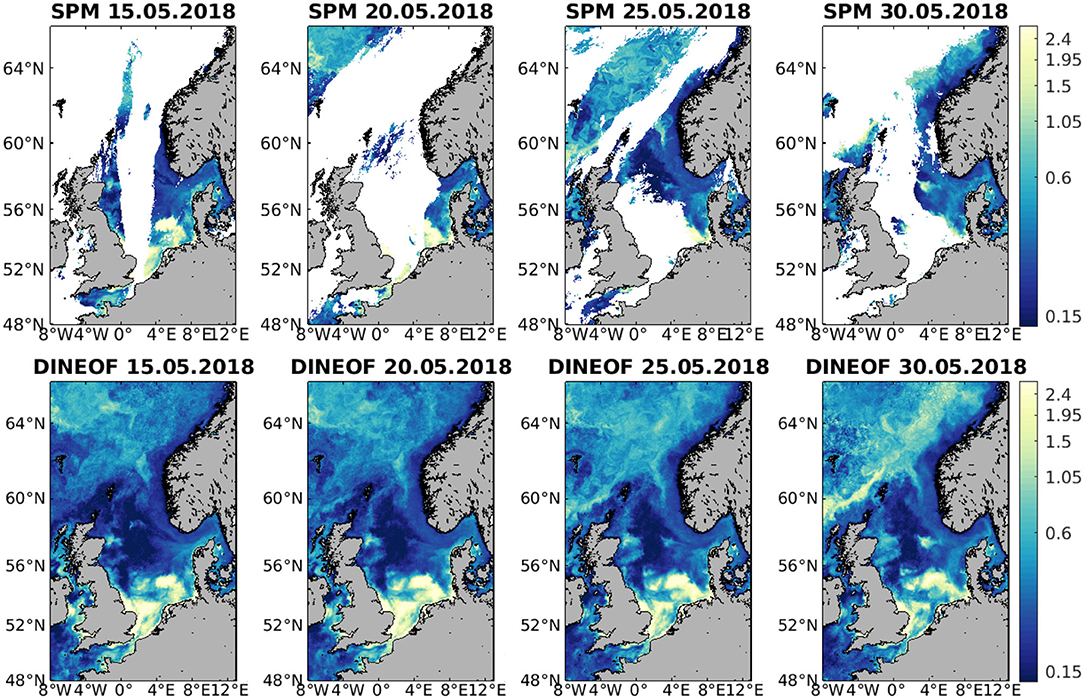
Figure 5. Example of SPM (mg/l) on 15, 20, 25, and 30 May 2018 for the initial data (top) and corresponding DINEOF reconstruction (bottom).

3.3. EOF Modes

The EOF modes that are provided by DINEOF have also been inspected for CHL (Figure 6) and SPM (Figure 7). In general, the first three modes display the same general patterns for all years, with obviously differences in small-scale patterns and intensity. As an illustration of the patterns represented in these modes, Figure 6 shows the first 4 EOF spatial and temporal modes in 2008 for CHL. The first EOF mode contains the seasonal variability due mainly to the spring bloom, as indicated by the first temporal mode showing a maximum in spring. The first spatial EOF mode has a larger amplitude along the coastal regions. The second EOF mode still shows a signal at the beginning of the year, indicating the CHL activity linked to the spring bloom, although this time in the center region of the North Sea. The third EOF appears to show the activity linked to blooms at higher latitudes, occurring for example around the Faroe Islands and peaking later in the year in the months of July and August. The fourth EOF is also included to show the smaller spatial and temporal variability included in the higher order modes.

FIGURE 6

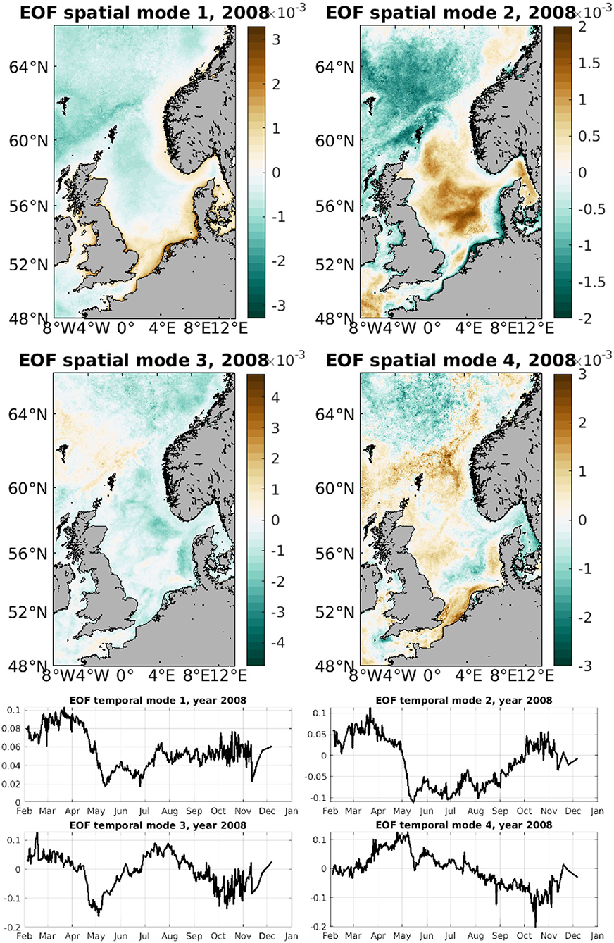
Figure 6. First four spatial CHL EOF modes for 2008 (top two rows) and first four temporal CHL EOF modes for 2008 (bottom two rows).

FIGURE 7

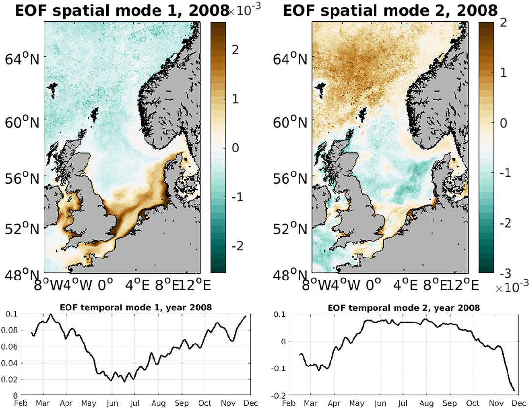
Figure 7. First two spatial SPM EOF modes for 2008 (top) and first two temporal SPM EOF modes for 2008 (bottom).

For SPM we only show the first 2 modes, as the higher order ones include small-scale variability and are therefore much more variable from year to year. Figure 7 shows the SPM spatial and temporal modes for 2008. The first spatial mode shows a larger amplitude in the southern coastal regions, which are shallower and receive large riverine discharges. The plume of the Thames river is also clearly seen, with high SPM values reaching several hundreds of km from its source. Maximum values, as expected, are found during the winter months (Figure 7). The second EOF mode highlights the central region of the North Sea, with higher SPM values again in winter. The southern coastal zones and the open sea waters in the north show a similar amplitude which peaks during summer months.

Given the high amount of data being analyzed, the correlation between the different EOF modes for the CHL data were also calculated. The aim was to examine in which years the CHL patterns are more similar to each other and which years the patterns of CHL are more different. Figure 8 shows the correlation between each year and all other years, for the first CHL EOF mode. The correlation matrix shows a diagonal with a correlation of 1 (correlation of each year CHL to itself), and symmetric values off the diagonal, with higher values for years with stronger correlation between them. The correlation between the first mode among all years is high (always higher than 0.8), as expected, since this mode shows the seasonal cycle as seen for example in Figure 6. However, we can also observe that there is a higher correlation among specific periods: the 1998–2001 period, the 2002–2012 period, the 2013–2016 period and the 2017–2020 period. As shown in Figure 2, the number of satellites used to compute the CHL data has been different through time, and this has an influence in the amount of missing data. The clusters of correlation shown in Figure 8 correspond well to changes in the total number of satellites available. Figure 8 also shows in the bottom panel the percentage of variability explained by the EOFs used in the DINEOF reconstruction, and this also reflects the changes in the number of satellites: analyses in years with one or two satellites have lower retained explained variability than years with three satellites. A similar result was observed in the first SPM EOF (not shown). This result seems to suggest that the availability of at least three ocean color satellites, providing better data coverage, results in improved representation of the variability by interpolation techniques, and sets up a target on the minimal requirements for a correct measurement of the ocean color variability.

FIGURE 8

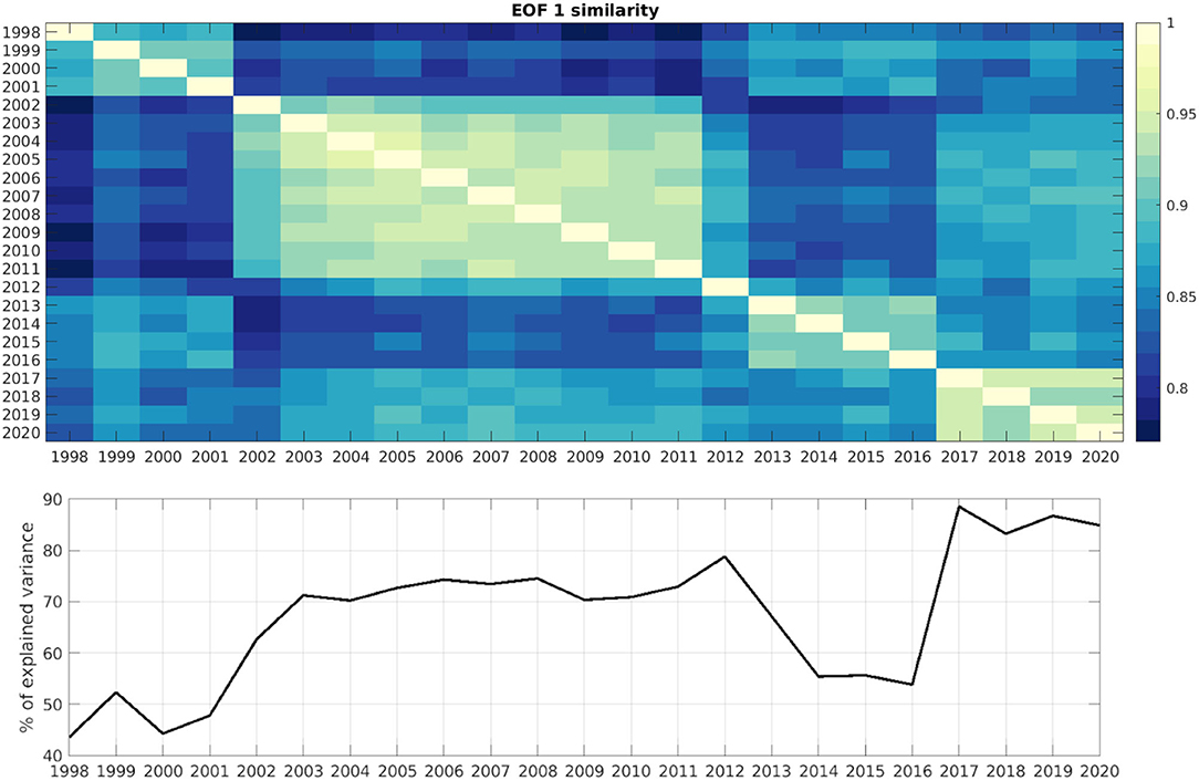
Figure 8. (Top) Correlation between each year first EOF CHL mode and all the other years. (Bottom) Percentage of explained variance retained in the DINEOF interpolated dataset.

3.4. Interannual Variability

A spatial average of the daily CHL and SPM products over the whole domain has been performed to assess interannual variability, and the time series has been filtered using a 30-day Gaussian low-pass filter (Figure 9). A large interannual variability in the average CHL value as well as in the strength of the spring peak can be observed. The reasons for this interannual variability are numerous, including variations in water temperature, water turbidity and nutrient availability (Desmit et al., 2020). The European Marine Strategy Framework Directive (MSFD), implemented in 2008, requires the European member states to achieve Good Environmental Status (GES), limiting for example the amount of nutrients that are shed to the rivers by agricultural activities. One of the consequences of this limitation in nutrients would be a decrease in the eutrophication of the North Sea, and in Figure 9 (top panel) it can indeed be observed that the average CHL concentration has decreased since 2008, with a stagnation, and even a slight increase, in recent years (2017–2020). Friedland et al. (2021) observed a decrease in CHL levels in the North Sea during the 2005–2012 period using an ensemble model simulation, and attributed this to a decrease in nutrient load from rivers into the North Sea. The highest CHL concentration in the average satellite time series of Figure 9 was reached in the spring bloom of 2008 (with 2.46 μg/l). The lowest concentration of CHL during the spring bloom in this same figure is observed in 2017 with 1.5 μg/l.

FIGURE 9

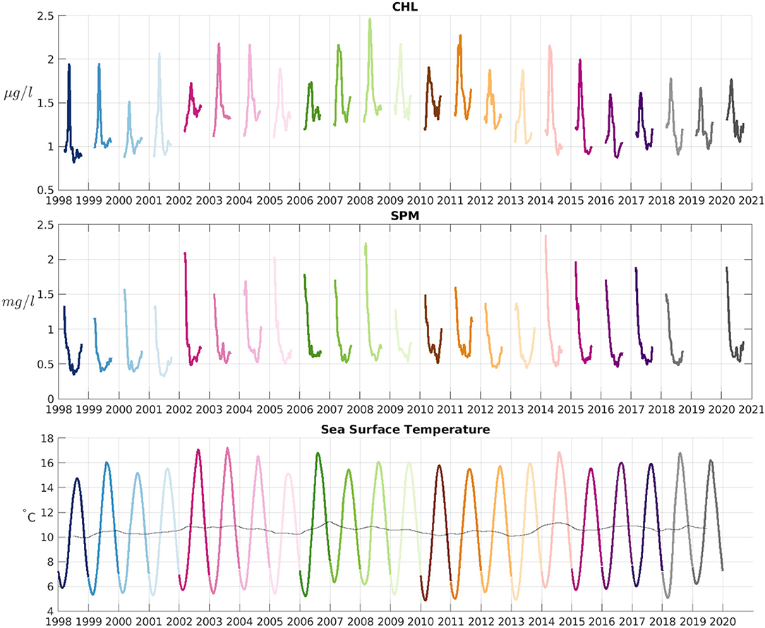
Figure 9. (Top) CHL Spatial average over the whole domain of Figure 1 during the 23 years of the study. (Middle) SPM averaged over the same region. Data from December-January is not plotted. (Bottom) SST spatial average over the whole domain. The thin black line shows the 1-yr running mean. Different colors for each year are used to ease comparison between variables for a given year. This color scheme is used in other multi-year figures in this work to ease comparison.

SPM time series (Figure 9, middle panel) shows a large variability in the winter values (with the time series starting in February of each year), when SPM reaches its highest values. Years like 2002, 2008, and 2014 show very high winter SPM concentrations, and in general the winter SPM average values have been higher in the periods 2002–2008 and 2014–2020 than in the rest of the time series. Minimum values are reached during summer months (Figure 9), when mixing and resuspension decreases. The interannual variability of the minimum values is not as high as the variability observed in maximum values.

4. Spring Bloom Onset

Following the threshold method described in section 2.4, we have calculated the date on which spring bloom starts each year. The dates of the spring bloom onset are shown in Figure 10. Despite interannual variability, there is a clear tendency at sooner spring bloom onset dates in recent years, i.e., the spring bloom appears to start on earlier dates. The trend toward earlier dates is significant with a p-value of 4.13e-05. A similar finding was already observed by Desmit et al. (2020) although their study was limited to the southern North Sea and used in situ data (i.e., the spatial extension was smaller). The date of the spring bloom onset has decreased 1.5 days per year in average over the studied period. The reasons for a change on the date of spring bloom onset can be varied. In the North Sea, as in the global ocean, water temperature has been increasing over the last decades as a result of climate change. For example, Desmit et al. (2020) reported an increase of the sea surface temperature in the North Sea of ~ 0.035°Cyr⁻¹ using in situ data from 1971 to 2014, and Høyer and Karagali (2016) found a 0.037°Cyr⁻¹ increment for the North Sea from 1982 to 2012 using a reanalysis product. Using CMEMS “European North West Shelf/Iberia Biscay Irish Seas - High Resolution L4 Sea Surface Temperature Reprocessed” Sea Surface Temperature (SST) satellite product, the daily average SST over the domain of study was calculated for the years 1998–2019 (last year available for this product at the moment of access), as shown in Figure 9. A warming of 0.31°C has been calculated from 1998 to 2019, or 0.015°Cyr⁻¹. This value differs from the others found in the references mentioned, but this difference can be attributed to the different spatial domains, periods considered and products used. All results however point at an increasing water temperature in the North Sea over the last decades. If nutrients are not limited, higher temperatures can accelerate phytoplankton cell division rates (e.g., Edwards et al., 2016; Hunter-Cevera et al., 2016), contributing to earlier blooms. The effect of rising temperature must be accompanied by a stratification of the water column to favor earlier blooms.

FIGURE 10

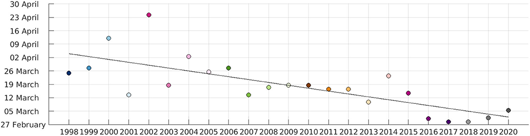
Figure 10. Date on which the CHL concentration reaches the annual median value for the first time each year. The solid black line shows a linear fit to the dates, with r = 0.75 and a p-value of 4.1267e-05.

The time of the spring bloom ending was also calculated following the opposite criterion as for the onset, i.e., the date on which the concentration of CHL first goes below the yearly median plus 5%. This is used to assess the duration of the spring bloom (time between onset and offset). While there is a high year-to-year variability in the duration of the spring bloom (Figure 11), a tendency toward longer blooms can be observed in more recent years, although this trend is not statistically significant. The years with longer bloom periods typically have a slow growing or weaning periods, as in 2013 and 2004, respectively (examples shown in Figure 11), causing the bloom period to be longer. Longer spring bloom periods do not mean higher CHL peaks or stronger blooms, and no significant correlation has been found between the strength of the peak (calculated as the difference between the maximum CHL value attained each year and the median value) and the duration of the bloom.

FIGURE 11

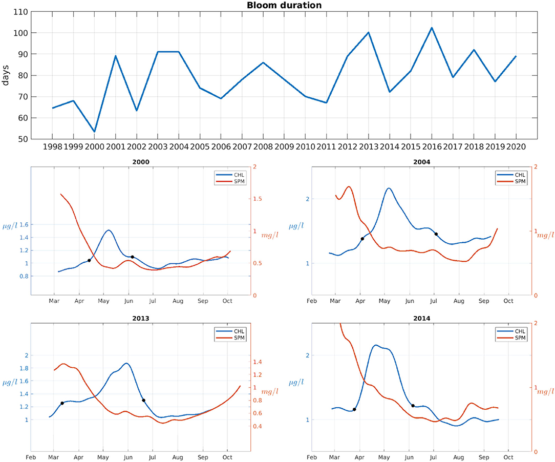
Figure 11. Top: spring bloom duration in days for each year of the study. Middle and bottom rows, the domain-averaged CHL (in blue) and SPM (in red) with a 30-day low pass filter. The dates at which the bloom starts and ends (black dots) as determined by the median threshold method. Years 2000, 2004, 2013, and 2014 are given as examples.

The average CHL concentration between the onset and offset of the bloom (Figure 12 top panel) shows increasing values during the period 1998–2008 and then a decreasing trend. Values in the 2017–2020 period are similar to what was observed during the early 2000s. Therefore, having spring blooms earlier in the year does not impact the average amount of CHL during the bloom. The amount of SPM during the winter months (February-March, as January is not used in our analysis because of the low availability of data) does not show a significant trend, but values appear in general to be higher during recent years. Studies of the influence of water clarity on phytoplankton growth reveal different results depending on the region. Several works (e.g., Capuzzo et al., 2015; Opdal et al., 2019; Wilson and Heath, 2019) found that light availability for phytoplankton growth has decreased on average in the North Sea during the XXth century through an increment of SPM. Philippart et al. (2013) on the other hand have found no significant increase or decrease of turbidity over four decades in the Wadden Sea (southeastern part of the North Sea). Our results do not show a clear trend in the average SPM concentration over the Greater North Sea over the period of study, so we cannot conclude that light availability has had an influence in the spring bloom onset date.

FIGURE 12

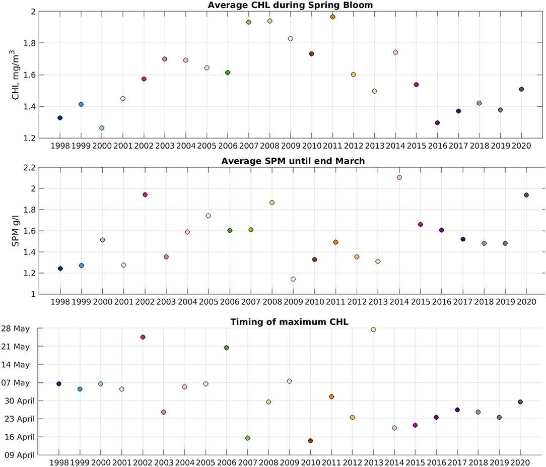
Figure 12. (Top) Average CHL during the spring bloom period each year. (Middle) Average SPM during February and March. (Bottom) Time at which the maximum CHL concentration is reached each year.

The time of maximum CHL concentration during each year bloom period has been also calculated (Figure 12 bottom panel). As the date of spring bloom onset has shifted to earlier dates, we could expect a similar shift in the peak of the bloom. While we can observe a general decrease in Figure 12 the variability is also high, specially during 2002–2013. The maximum CHL concentration during recent years (2014–2020) is reached 1–2 weeks earlier than what was observed in the early 2000s. While the linear trend over all the years is not significant (p = 0.07), it would be worth revisiting this when more data become available, to determine if there is a shift in the date when the spring bloom reaches its maximum.

The data presented show that the spring bloom in the Greater North Sea has shifted to earlier dates during the last 23 years, with the maximum CHL value probably occurring also in earlier dates. Bloom duration shows high variability but appears to have become longer, but the average amount of CHL during the spring bloom period does not show a clear trend over time, indicating that the blooms have not become stronger nor weaker due to the shift in time. From all the analyses shown in Figures 10–12, only the date on which the spring bloom starts each year (i.e., Figure 10) shows a statistically significant trend. SPM values during winter months show also higher values during more recent years, although there is a lot of variability in these data. Higher SPM would imply lower CHL or later spring bloom onset dates as more turbid waters hinder light availability for primary producers. We therefore suggest that the role of increasing water temperature has had a stronger effect in spring bloom onset date than SPM concentration. However, given the large size of the domain of study, multiple factors are probably responsible for the observed change in spring bloom onset date, with the relative influence of each factor probably varying in each region.

5. Conclusions

We have performed a daily, gap-free reconstruction of chlorophyll (CHL) and suspended particulate matter (SPM) in the Greater North Sea region over the period 1998 to 2020 with a spatial resolution of 1 km. Missing data have been reconstructed using DINEOF (Data Interpolating Empirical Orthogonal Functions). The mesoscale variability observed in the initial, gappy data (eddies, fronts, Thames river plume) are retained in the final datasets, demonstrating the high resolution of the reconstructed data. Both the initial and reconstructed data were validated in Van der Zande et al. (2019b) and showed a correct level of accuracy. The EOF modes used for the reconstruction show that, in general, the southern part of the domain has the largest variability. This is due in part to the shallower depths, and the largely urbanized coasts of this region which result in more nutrients reaching the coastal waters through river run-off.

The interannual variability was observed to be high, with changes in year-to-year CHL and SPM annual cycle, as well as their maximum and minimum values. Maximum CHL values obtained during the spring bloom have increased during the period 1998–2008, and show a decrease during 2008–2017. The maximum CHL appears to be slightly increasing again during the period 2017–2020.

This work has shown that the start date of the spring bloom occurs earlier every year in the North Sea, with starting dates in 2020 about 1 month earlier than in 1998. Earlier spring bloom dates have been described in the southern part of the North Sea using in situ data (Desmit et al., 2020), and our study has shown this trend on a global scale covering the Greater North Sea, using satellite data. Increasing water temperatures can explain at least in part this trend, although it remains unclear what the role of the SPM has been. The SPM average concentration in February-March each year does not show a clear trend that could help explain the earlier dates of the spring bloom.

Another major conclusion of this work is related to the use of a variable number of satellites in long-term ocean color analyses, and the impact of this number in the final product. The number of satellites used to compute CHL and SPM has an impact in the amount of explained variance by the EOF modes used in DINEOF, as more satellites provide also a better spatio-temporal coverage of all scales of variability. In order to retain a large amount of the initial variability, at least three satellites measuring ocean color are required. Periods with only 1 or 2 satellites showed a lower amount of percentage of retained variance in the final, interpolated product. This result sets up a target on the minimal number of satellites that would be needed for a correct measurement of the ocean color variability, specially in zones with a high amount of clouds and other sources of missing data.

Analysis of long time series of CHL and SPM data are necessary to understand the impact of human activities on the ecosystem. Using gap-free satellite data at high spatial resolution is necessary to resolve the small-scale variability that contributes to the net variations of CHL and SPM, and our DINEOF analysis of these variables has been shown to provide enough detail to resolve these structures. Due to the large size of the domain of study, with shallow waters in the southern, highly populated region, an open connection to the Atlantic Ocean to the North, and the opening to the Baltic sea to the East, the factors influencing spring bloom phenology can be also multiple. Future work should address the changes observed in sub-regions of the North Sea, like the Southern North Sea, the Norwegian channel or the Faroe Islands.

Data Availability Statement

The raw data supporting the conclusions of this article will be made available by the authors, without undue reservation.

Author Contributions

AA-A realized the reconstruction analyses, made the figures, and wrote the manuscript. DV prepared the initial data, did the validation and contributed to discussion, and writing of the manuscript. AB contributed to the interpretation of the results, the discussion, and the writing of the manuscript. CT contributed to the discussion and the writing of the manuscript. SM contributed to the discussion and the writing of the manuscript. J-MB contributed to the discussion and the writing of the manuscript. All authors contributed to the article and approved the submitted version.

Conflict of Interest

The authors declare that the research was conducted in the absence of any commercial or financial relationships that could be construed as a potential conflict of interest.

Publisher's Note

All claims expressed in this article are solely those of the authors and do not necessarily represent those of their affiliated organizations, or those of the publisher, the editors and the reviewers. Any product that may be evaluated in this article, or claim that may be made by its manufacturer, is not guaranteed or endorsed by the publisher.

Acknowledgments

This research was performed with funding from the Belgian Science Policy Office (BELSPO) STEREO III programme in the framework of the MULTI-SYNC project (contract SR/00/359). Computational resources have been provided by the Consortium des Équipements de Calcul Intensif (CÉCI), funded by the Fonds de la Recherche Scientifique de Belgique (F.R.S.-FNRS) under Grant No. 2.5020.11 and by the Walloon Region.

References

Alvera-Azcárate, A., Barth, A., Beckers, J.-M., and Weisberg, R. H. (2007). Multivariate reconstruction of missing data in sea surface temperature, chlorophyll and wind satellite fields. J. Geophys. Res. 112:C03008. doi: 10.1029/2006JC003660

CrossRef Full Text | Google Scholar

Alvera-Azcárate, A., Barth, A., Parard, G., and Beckers, J.-M. (2016). Analysis of SMOS sea surface salinity data using DINEOF. Remote Sens. Environ. 180, 137–145. doi: 10.1016/j.rse.2016.02.044

CrossRef Full Text | Google Scholar

Alvera-Azcárate, A., Barth, A., Rixen, M., and Beckers, J.-M. (2005). Reconstruction of incomplete oceanographic data sets using empirical orthogonal functions. Application to the Adriatic Sea surface temperature. Ocean Modell. 9, 325–346, doi: 10.1016/j.ocemod.2004.08.001

CrossRef Full Text | Google Scholar

Alvera-Azcárate, A., Barth, A., Sirjacobs, D., and Beckers, J.-M. (2009). Enhancing temporal correlations in EOF expansions for the reconstruction of missing data using DINEOF. Ocean Science 5, 475–485. doi: 10.5194/os-5-475-2009

CrossRef Full Text | Google Scholar

Alvera-Azcárate, A., Vanhellemont, Q., Ruddick, K., Barth, A., and Beckers, J.-M. (2015). Analysis of high frequency geostationary ocean colour data using DINEOF. Estuar. Coast. Shelf Sci. 159, 28–36. doi: 10.1016/j.ecss.2015.03.026

CrossRef Full Text | Google Scholar

Bailey, S., and Werdell, P. (2006). A multi-sensor approach for the on-orbit validation of ocean color satellite data products. Remote Sens. Environ. 102, 12–23. doi: 10.1016/j.rse.2006.01.015

CrossRef Full Text | Google Scholar

Beckers, J.-M., Barth, A., and Alvera-Azcárate, A. (2006). DINEOF reconstruction of clouded images including error maps. Application to the sea surface temperature around Corsican Island. Ocean Sci. 2, 183–199. doi: 10.5194/os-2-183-2006

CrossRef Full Text | Google Scholar

Beckers, J.-M., and Rixen, M. (2003). EOF calculations and data filling from incomplete oceanographic data sets. J. Atmos. Ocean. Technol. 20, 1839–1856. doi: 10.1175/1520-0426(2003)020<1839:ECADFF>2.0.CO;2

CrossRef Full Text | Google Scholar

Brody, S. R., Lozier, M. S., and Dunne, J. P. (2013). A comparison of methods to determine phytoplankton bloom initiation. J. Geophys. Res. Oceans 118, 2345–2357. doi: 10.1002/jgrc.20167

CrossRef Full Text | Google Scholar

Capuzzo, E., Lynam, C. P., Barry, J., Stephens, D., Forster, R. M., Greenwood, N., et al. (2017). A decline in primary production in the north sea over 25 years, associated with reductions in zooplankton abundance and fish stock recruitment. Glob. Change Biol. 24, 1–13. doi: 10.1111/gcb.13916

PubMed Abstract | CrossRef Full Text | Google Scholar

Capuzzo, E., Stephens, D., Silva, T., Barry, J., and Forster, R. M. (2015). Decrease in water clarity of the southern and central North Sea during the 20th century. Glob. Change Biol. 21, 2206–2214. doi: 10.1111/gcb.12854

PubMed Abstract | CrossRef Full Text | Google Scholar

Desmit, X., Nohe, A., Borges, A.-V., Prins, T., De Cauwer, K., Lagring, R., et al. (2020). Changes in chlorophyll concentration and phenology in the North Sea in relation to de-eutrophication and sea surface warming. Limnol. Oceanogr. 65, 828–847. doi: 10.1002/lno.11351

CrossRef Full Text | Google Scholar

Desmit, X., Ruddick, K., and Lacroix, G. (2015). Salinity predicts the distribution of chlorophyll a spring peak in the southern North Sea continental waters. J. Sea Res. 103, 59–74. doi: 10.1016/j.seares.2015.02.007

CrossRef Full Text | Google Scholar

Ducrotoy, J. P., Elliott, M., and Jonge, V. N. (2000). The North Sea. Mar. Pollut. Bull. 41, 5–23. doi: 10.1016/S0025-326X(00)00099-0

CrossRef Full Text | Google Scholar

Edwards, K. F., Thomas, M. K., Klausmeier, C. A., and Litchman, E. (2016). Phytoplankton growth and the interaction of light and temperature: a synthesis at the species and community level. Limnol. Oceanogr. 61, 1232–1244. doi: 10.1002/lno.10282

CrossRef Full Text | Google Scholar

Ferrari, R., Merrifield, S. T., and Taylor, J. R. (2015). Shutdown of convection triggers increase of surface chlorophyll. J. Mar. Syst. 147, 116–122. doi: 10.1016/j.jmarsys.2014.02.009

CrossRef Full Text | Google Scholar

Ferreira, J., Andersen, J., Borja, A., Bricker, S., Camp, J., Cardoso da Silva, M., et al. (2011). Overview of eutrophication indicators to assess environmental status within the European Marine Strategy Framework Directive. Estuar. Coast. Shelf Sci. 93, 117–131. doi: 10.1016/j.ecss.2011.03.014

CrossRef Full Text | Google Scholar

Fettweis, M., Baeye, M., Van der Zande, D., Van den Eynde, D., and Lee, J. (2014). Seasonality of floc strength in the southern North Sea. J. Geophys. Res. Oceans 119, 1911–1926. doi: 10.1002/2013JC009750

CrossRef Full Text | Google Scholar

Fettweis, M., Nechad, B., and den Eynde, D. V. (2007). An estimate of the suspended particulate matter (SPM) transport in the southern North Sea using SeaWiFS images, in situ measurements and numerical model results. Continent. Shelf Res. 27, 1568–1583. doi: 10.1016/j.csr.2007.01.017

CrossRef Full Text | Google Scholar

Friedland, R., Macias, D., Cossarini, G., Daewel, U., Estournel, C., Garcia-Gorriz, E., et al. (2021). Effects of nutrient management scenarios on marine eutrophication indicators: a pan-European, multi-model assessment in support of the marine strategy framework directive. Front. Mar. Sci. 8:596126. doi: 10.3389/fmars.2021.596126

CrossRef Full Text | Google Scholar

Gohin, F., Druon, J. N., and Lampert, L. (2002). A five channel chlorophyll concentration algorithm applied to SeaWiFS data processed by SeaDAS in coastal waters. Int. J. Remote Sens. 23, 1639–1661. doi: 10.1080/01431160110071879

CrossRef Full Text | Google Scholar

Gons, H. J., Rijkeboer, M., and Ruddick, K. G. (2002). A chlorophyll-retrieval algorithm for satellite imagery (Medium Resolution Imaging Spectrometer) of inland and coastal waters. J. Plankton Res. 24, 947–951. doi: 10.1093/plankt/24.9.947

CrossRef Full Text | Google Scholar

Høyer, J., and Karagali, I. (2016). Sea surface temperature climate data record for the North Sea and Baltic Sea. J. Clim. 29, 2529–2541. doi: 10.1175/JCLI-D-15-0663.1

CrossRef Full Text | Google Scholar

Huisman, J., van Oostveen, P., and Weissing, F. J. (1999). Critical depth and critical turbulence: Two different mechanisms for the development of phytoplankton blooms. Limnol. Oceanogr. 44, 1781–1787.

Google Scholar

Hunter-Cevera, K. R., Neubert, M. G., Olson, R. J., Solow, A. R., Shalapyonok, A., and Sosik, H. M. (2016). Physiological and ecological drivers of early spring blooms of a coastal phytoplankter. Science 354, 326–329. doi: 10.1126/science.aaf8536

PubMed Abstract | CrossRef Full Text | Google Scholar

Huynh, T. H. N., Alvera-Azcárate, A., and Beckers, J.-M. (2020). Analysis of surface chlorophyll a associated with sea surface temperature and surface wind in the South China Sea. Ocean Dyn. 70, 139–161. doi: 10.1007/s10236-019-01308-9

CrossRef Full Text | Google Scholar

Kröncke, I. (2011). Changes in Dogger Bank macrofauna communities in the 20th century caused by fishing and climate. Estuar. Coast. Shelf Sci. 94, 234–245.

Google Scholar

Lancelot, C., Spitz, Y., Gypens, N., Ruddick, K., Becquevort, S., Rousseau, V., et al. (2005). Modelling diatom and Phaeocystis blooms and nutrient cycles in the Southern Bight of the North Sea: the MIRO model. Mar. Ecol. Prog. Ser. 289, 63–78. doi: 10.3354/meps289063

CrossRef Full Text | Google Scholar

Lavigne, H., Van der Zande, D., Ruddick, K., Cardoso Dos Santos, J., Gohin, F., Brotas, V., et al. (2021). Quality-control tests for OC4, OC5 and NIR-red satellite chlorophyll-a algorithms applied to coastal waters. Remote Sens. Environ. 255:112237. doi: 10.1016/j.rse.2020.112237

CrossRef Full Text | Google Scholar

Nechad, B., Ruddick, K., and Park, Y. (2010). Calibration and validation of a generic multisensor algorithm for mapping of total suspended matter in turbid waters. Remote Sens. Environ. 114, 854–866. doi: 10.1016/j.rse.2009.11.022

CrossRef Full Text | Google Scholar

Opdal, A. F., Lindemann, C., and Aksnes, D. L. (2019). Centennial decline in north sea water clarity causes strong delay in phytoplankton bloom timing. Glob. Change Biol. 25, 3946–3953. doi: 10.1111/gcb.14810

PubMed Abstract | CrossRef Full Text | Google Scholar

O'Reilly, J. E., Maritorena, S., Mitchell, B., Siegel, D., Carder, K. L., Garver, S. A., et al. (1998). Ocean color chlorophyll algorithms for SeaWiFS. J. Geophys. Res. Oceans 103, 24937–24953.

Google Scholar

Philippart, C., Salama, M. S., Kromkamp, J. C., van der Woerd, H. J., Zuur, A. F., and Cadee, G. C. (2013). Four decades of variability in turbidity in the western Wadden Sea as derived from corrected Secchi disk readings. J. Sea Res. 82, 67–79. doi: 10.1016/j.seares.2012.07.005

CrossRef Full Text | Google Scholar

Philippart, C., van Iperen, J., Cadee, G., and Zuur, A. (2010). Long-term field observations on seasonality in chlorophyll-a concentrations in a shallow coastal marine ecosystem, the Wadden Sea. Estuar. Coasts 33, 286–294. doi: 10.1007/s12237-009-9236-y

CrossRef Full Text | Google Scholar

Rousseau, V., Lantoine, F., Rodriguez, F., LeGall, F., Chretiennot-Dinet, M.-J., and Lancelot, C. (2013). Characterization of Phaeocystis globosa (Prymnesiophyceae), the blooming species in the Southern North Sea. J. Sea Res. 76, 105–113. doi: 10.1016/j.seares.2012.07.011

CrossRef Full Text | Google Scholar

Sathyendranath, S., Brewin, R., Brockmann, C., Brotas, V., Calton, B., Chuprin, A., et al. (2019). An ocean-colour time series for use in climate studies: the experience of the ocean-colour climate change initiative (OC-CCI). Sensors 19:4285. doi: 10.3390/s19194285

PubMed Abstract | CrossRef Full Text | Google Scholar

Schroeder, T., Schaale, M., and Fischer, J. (2007). Retrieval of atmospheric and oceanic properties from MERIS measurements: a new Case-2 water processor for BEAM. Int. J. Remote Sens. 28, 5627–5632. doi: 10.1080/01431160701601774

CrossRef Full Text | Google Scholar

Sirjacobs, D., Alvera-Azcárate, A., Barth, A., Lacroix, G., Park, Y., Nechad, B., et al. (2011). Cloud filling of ocean color and sea surface temperature remote sensing products over the Southern North Sea by the Data Interpolating Empirical Orthogonal Functions methodology. J. Sea Res. 65, 114–130. doi: 10.1016/j.seares.2010.08.002

CrossRef Full Text | Google Scholar

Sündermann, J., and Pohlmann, T. (2011). A brief analysis of North Sea physics. Oceanologia 53, 663–689. doi: 10.5697/oc.53-3.663

CrossRef Full Text | Google Scholar

Van der Zande, D., Eleveld, M., Lavigne, H., Gohin, F., Pardo, S., Tilstone, G., et al. (2019a). Joint Monitoring Programme of the EUtrophication of the NOrth Sea with SATellite data user case in Copernicus Marine Service Ocean State Report. J. Operat. Oceanogr. 12, 1–123. doi: 10.1080/1755876X.2019.1633075

CrossRef Full Text | Google Scholar

Van der Zande, D., Lavigne, H., Blauw, A., Prins, T., Desmit, X., Eleveld, M., et al. (2019b). Enhance Coherence in Eutrophication Assessments Based on Chlorophyll, Using Satellite Data as Part of the EU Project–Joint Monitoring Programme of the Eutrophication of the North Sea With Satellite Data (JMP-EUNOSAT). Technical report, RBINS. Available online at: https://www.informatiehuismarien.nl/projecten/algaeevaluated/information/results/

Vindenes, H., Orvik, K., Søiland, H., and Wehde, H. (2018). Analysis of tidal currents in the North Sea from shipboard acoustic Doppler current profiler data. Continent. Shelf Res. 162, 1–12. doi: 10.1016/j.csr.2018.04.001

CrossRef Full Text | Google Scholar

von Storch, H., and Zwiers, F. W. (1999). Statistical Analysis in Climate Research. Cambridge: Cambridge University Press, 484. doi: 10.1017/CBO9780511612336

CrossRef Full Text | Google Scholar

Wilson, R. J., and Heath, M. R. (2019). Increasing turbidity in the north sea during the 20th century due to changing wave climate. Ocean Sci. 15, 1615–1625. doi: 10.5194/os-15-1615-2019

CrossRef Full Text | Google Scholar

Winther, N. G., and Johannessen, J. A. (2006). North Sea circulation: Atlantic inflow and its destination. J. Geophys. Res. Oceans 111:C12. doi: 10.1029/2005JC003310

CrossRef Full Text | Google Scholar

Xu, X., Lemmen, C., and Wirtz, K. W. (2020). Less nutrients but more phytoplankton: long-term ecosystem dynamics of the Southern North Sea. Front. Mar. Sci. 7:662. doi: 10.3389/fmars.2020.00662

CrossRef Full Text | Google Scholar