Climate Signals in the Black Sea From a Multidecadal Eddy-Resolving Reanalysis

Introduction

The Black Sea is the largest land-locked basin in the world with an area of 4.2 × 10⁵ km², a volume of 5.3 × 10⁵ km³ and a maximum depth of 2200 m (Özsoy and Ünlüata, 1997). It is connected to the Marmara Sea and Azov Sea through the straits of Bosphorus and Kerch, respectively. It is an estuarine basin, characterized by a positive net freshwater balance, mainly due to the outflow of some of the largest European rivers such as the Danube and Dniepr, and a high-rate of precipitation which in total exceeds the total evaporation most of the time over the basin (Kara et al., 2008; Volkov and Landerer, 2015). The resulting salinity of about 18 psu in the upper layer forms a strong stratification all over the basin where a saltier water of Mediterranean origin, crossing the Marmara Sea and the Bosphorus Strait, becomes the major source of ventilation for the anoxic lower layer (Ünlülata et al., 1990; Stanev and Beckers, 1999; Stanev et al., 2001). Another main characteristic of the Black Sea is the Cold Intermediate Layer (CIL) formed at the depth of the winter convection (Özsoy and Ünlüata, 1997). The upper layer circulation of the Black Sea is dominated by the Rim Current, a quasi-permanent cyclonic jet following the bottom topography which interacts with several anti-cyclonic eddies (e.g., Batumi and Sevastopol) along its pathway in the basin (Oguz et al., 1993; Korotaev et al., 2003).

The evolution of remote sensing has been crucial to understand some of the above-mentioned Black Sea processes, since it provides high temporal and spatial resolution observations (Korotaev et al., 2001). Kubryakov and Stanichny (2015) investigated the seasonal and interannual variability of the Black Sea eddies and found a relationship between the eddy properties and the intensity of the Rim Current using altimeter observations. In addition, sea surface temperature observations have helped to detect recent warming in the Black Sea as a response of climate change (Ginzburg et al., 2004; Shapiro et al., 2010; Mulet et al., 2018). However, the major challenge for studying the ocean dynamics in the Black Sea is the historical scarcity of sub-surface observations. Although this situation has been improved in the recent years with the first deployment of Argo floats after 2002 (Grayek et al., 2015), the number of in-situ observations significantly increased only after 2010. For instance, profiling floats contributed to the detection of a recent warming in the Black Sea and the reduction of the cold-water content in the CIL (Akpinar et al., 2017; Stanev et al., 2019).

Numerical ocean models represent a powerful complementary tool to investigate the three-dimensional state of the Black Sea circulation in time in absence of dense observations. Kara et al. (2005) used an eddy-resolving model to investigate the effects of ocean turbidity on upper-ocean circulation features including sea surface height and mixed layer depth. From a 56-year model simulation, Miladinova et al. (2017) revealed that temperature has a seasonal cycle at the surface, decreasing with depth down to the CIL. Next, the same simulation was used to investigate the formation and changes of the CIL and revealed that the cooling capacity of the CIL is highly variable and decreased drastically in the last decade of the simulation (Miladinova et al., 2018). Gunduz et al. (2020) related the reduced events of CIL formation in recent years to the amplified response to climate change of the Black Sea. Although current ocean models are highly sophisticated, including improvements in parameterization of physical processes of unresolved scale and incorporating numerical techniques that are optimal for ocean regions dynamically different, they still have some limitations and incorporate uncertainties from several sources (Lima et al., 2019). Therefore, they are not completely appropriate for providing accurate ocean monitoring indicators when used alone, nor to fully study the oceanic dynamics in the Black Sea.

Ocean reanalyses reconstruct the ocean state with a long integration of an ocean model constrained by atmospheric surface forcing and observations via data assimilation (Haines, 2018; Storto et al., 2019a). They provide a four-dimensional time series of the ocean state to study ocean dynamics and unravel sources and impacts of ocean variability. Ocean reanalyses can also provide initial and boundary conditions to other models as in downscaling simulations (de Souza et al., 2020) and uncoupled seasonal forecast initializations (Balmaseda, 2017). In the Black Sea, Knysh et al. (2011) conducted a pioneering investigation utilizing an ocean reanalysis. They applied a simple data assimilation scheme to ingest available in-situ observations from 1971 to 1993.

In this work we present a Black Sea reanalysis (BS-REA) that covers the altimeter era starting from 1993 until 2018. This reanalysis system has been continuously developed in the scope of the Copernicus Marine Environment Monitoring Service (CMEMS, Le Traon et al., 2019) since 2016 (Lima et al., 2020b). It is based on an eddy-resolving ocean model coupled with an advanced data assimilation scheme, which is very innovative for the Black Sea region. Here, we present a recently upgraded version in both model and data assimilation components, which we believe will help the community for a better understanding of the physical properties and dynamics of the Black Sea. Our objective is to ensure the best representation of the sea circulation and its thermohaline structure, as well as to provide more accurate ocean monitoring indicators that can help to understand the Black Sea response to climate change.

This article was organized as follows: in section 2 we outline the BS-REA configuration in detail; in section 3 we present the main characteristics of the BS-REA and discuss the results, and finally in section 4 the conclusions are drawn.

BS-REA Configuration

Ocean Model

The present BS-REA hydrodynamic model is configured for the Black Sea region (the Azov Sea is not included) and it is based on NEMO v3.6 implicit free-surface implementation (Madec and The Nemo team, 2016), with a horizontal resolution of 1/27° in the zonal direction and 1/36° in the meridional direction, and 31 unevenly spaced vertical z-levels. This horizontal spatial resolution is chosen in order to have the same cartesian resolution in latitudinal and longitudinal directions, around 3 km at the model domain latitudes, which is conformed to an eddy-resolving scale; the Rossby radius of deformation in the Black Sea is approximately 20 km (Hallberg, 2013). The BS-REA horizontal spatial domain is shown in Figure 1.

FIGURE 1

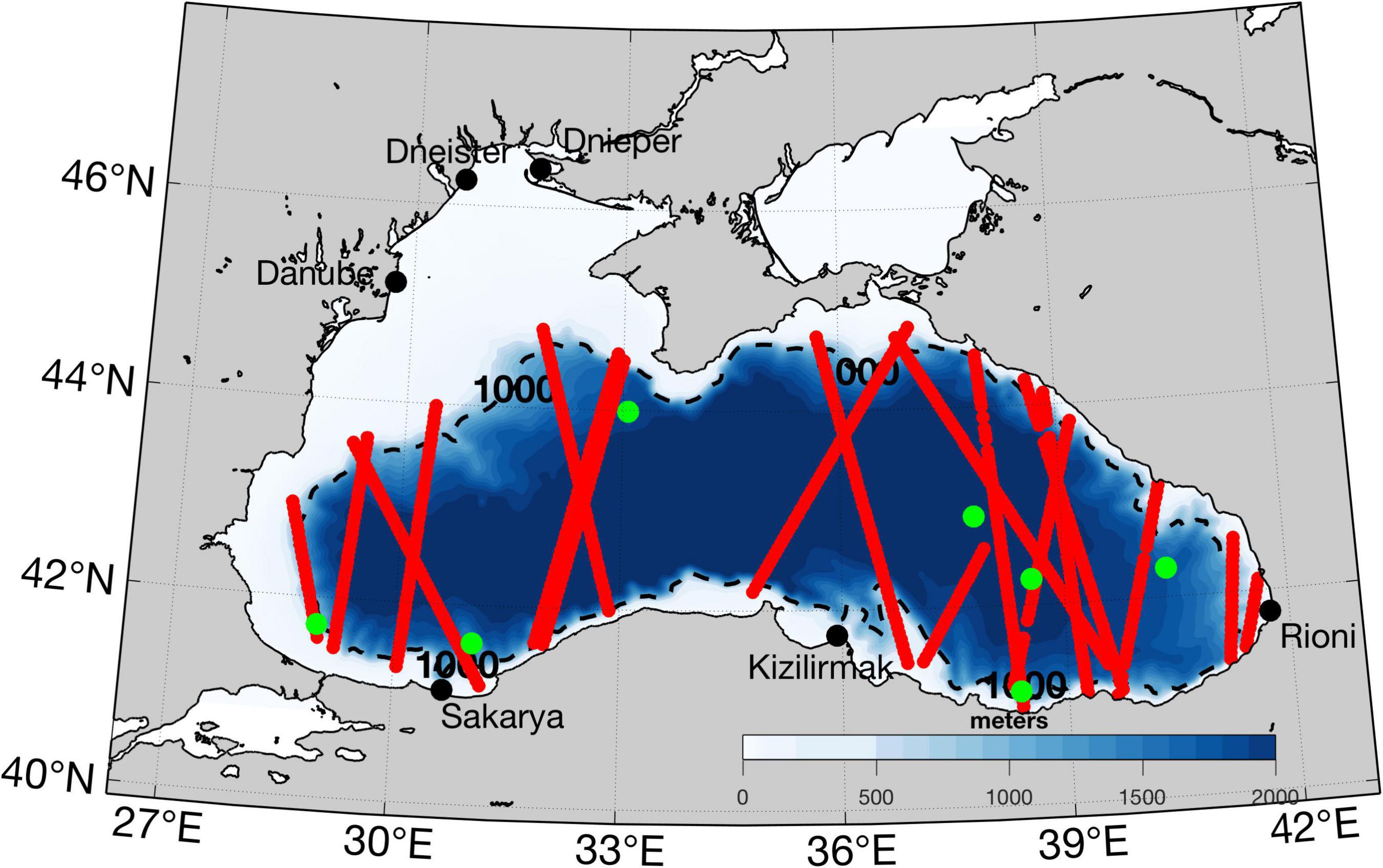
Figure 1. Black Sea spatial domain and bathymetry. The red lines indicate the sea level anomaly along-track and green dots indicate the T and S in situ profiles available for data assimilation within the 4-day observation window on 18 October 2018.

The model is forced by the ECMWF ERA-5 atmospheric reanalysis (Hersbach et al., 2020) at the surface with a 0.25° of spatial resolution and 1-hour time frequency. The atmospheric forcing variables are: the zonal and meridional components of 10 m wind (in m s^–1), total cloud cover (in %), 2 m air temperature (in K), 2 m dew point temperature (in K) and mean sea level pressure (in Pa). Precipitation (in kg/m² s) over the basin is obtained from GPCP rainfall monthly database (Adler et al., 2003; Huffman et al., 2009), from which monthly climatological means are estimated considering the period 1979–2019. The momentum, heat and water fluxes are computed at the air-sea interface based on the bulk formulae originally developed for the Mediterranean Sea (Castellari et al., 1998; Pettenuzzo et al., 2010) and applied as in the Black Sea forecasting system (Ciliberti et al., 2020).

The model bathymetry is based on the GEBCO gridded dataset at 30” resolution¹ in the Black Sea basin. The bathymetry is improved around the Bosphorus Strait with a high-resolution dataset, extensively described in Gürses (2016). Once acquired the high-resolution dataset, an optimal barycentric interpolation method is used to interpolate scattered bathymetric data on the regular spatial grid. The coastline is revised to account for and properly represents the coastal peculiarities and structures in the basin by using the NOAA shoreline dataset². The river locations are remapped considering the new bathymetry.

For the river runoff, we use a monthly climatological mean estimate for the period 1960–1984 and provided by the SESAME project (Ludwig et al., 2009). The total number of rivers is 72, including the major ones such as Danube, Dnieper, Rioni, Dniester, Sakarya and Kizilirmak. The Danube runoff is distributed over five grid points to better represent its major branches, i.e., Chilia, Sulina, St. George. This special treatment accounts that the Chilia is the greatest one with three sub-branches. One is located in the south, in the Romanian territory, while the other two are in Ukraine. Sulina and St. George are located in the larger Danube floodplain, which occupies around 3500 km². Thus, the distribution of the Danube discharge over its three main branches follows Panin et al. (2016); the Chilia spread 52% of the total discharge, while the remaining 48% is distributed in the Sulina (20%) and St. George (28%) branches, respectively. The salinity of the river waters is assumed to be zero.

Since the current model configuration of the BS-REA has closed lateral boundaries, the Bosphorus Strait net transport is parameterised as a river by means of surface boundary conditions while temperature and salinity are relaxed to a previous estimate. The net transport is computed iteratively from a simulation and a series of assimilation runs. A first iteration, which is a simulation, adopts a monthly climatology (Kara et al., 2008) and integrates for the whole reanalysis period. Then, every following iteration imposes the net outflow corrected by E-P-R estimates from the previous one in order to balance the water budget; evaporation (E) is model-derived and depends on each integration whereas precipitation (P) and river runoff (R) are monthly climatology as described above. In the BS-REA, a final correction, estimated from the CMEMS SSALTO/DUACS Delayed-Time Level-4 sea level anomalies measured by multi-satellite altimetry observations (Taburet et al., 2019), is applied to the freshwater balance at a single grid point adjacent to the Bosphorus Strait in order to impose the observed trend and variability in the mean sea surface height. T and S are relaxed toward a monthly climatological profile computed from a high-resolution multi-year simulation (Aydoğdu et al., 2018), to properly represent the water mass properties exchanged between the Mediterranean and Black Seas via the Bosphorus Strait. This relaxation is applied at five grid points surrounding the location of the Bosphorus Strait with a time frequency of 1 hour.

Finally, we restore the SST over the basin to the gridded CMEMS SST product (Buongiorno Nardelli et al., 2013). The restoring is done by added a damping term to the surface heat flux with a constant coefficient of dQ/dT = −200 W/m²/K.

Observations

The BS-REA assimilates sea level anomaly (SLA), temperature and salinity observations. The specific products assimilated are: (i) in-situ T/S profiles from both SeaDataNet³ (Pecci et al., 2020) and CMEMS NRT in-situ product (von Schuckmann et al., 2016) and (ii) along-track sea level anomaly from all available missions, pre-processed and distributed by the CMEMS Sea Level TAC (Taburet et al., 2019). For SLA assimilation, the choice of the mean dynamic topography (MDT) is a key point and can impact the quality of results (Yan et al., 2015). In BS-REA, a model-based MDT is computed using a 20-year (1993–2012) mean of sea surface height derived from a model integration with the assimilation of T and S profiles only.

The in-situ instrumental errors assume different values for T and S and vary in the vertical dimension based on statistics derived from Ingleby and Huddleston (2007), whereas the in-situ representation errors vary horizontally on the model grid according to previous model statistics with respect to observations and adopt same values for T and S. Both components of in situ errors are constant over time. For SLA observations, the instrumental error is set to 4 cm, and the representation errors monthly and spatially vary following Oke and Sakov (2008).

Data Assimilation Scheme

The data assimilation scheme is the OceanVar (Dobricic and Pinardi, 2008; Storto et al., 2011), a three-dimensional variational (3D-Var) assimilation algorithm. The 3D-Var scheme aims to iteratively find an optimal analysis field, x_a, that minimizes a cost function (Eq. 1).

$$J=\frac{1}{2}\mathrm{\delta }{x}^T{B}^{-1}\mathrm{\delta }x+\frac{1}{2}{\left(H\mathrm{\delta }x-d\right)}^T{R}^{-1}\left(H\mathrm{\delta }x-d\right)(1)$$

δx = x − x_b, where x is the unknown ocean state, equal to the analysis x_a at the minimum of J, x_b is the background state, d = y − H (x_b) is the misfit between an observation y and its modeled correspondent (in the observation space) where H, the observation operator, maps the model fields at the observation location. The method accounts for the background and observation uncertainties through the error covariance matrices B and R, respectively. The observational error covariance matrix R is diagonal in the observation space and includes the sum of instrumental and representation errors and an error component according to the time of each observation with respect to the analysis time, i.e., the observation error is multiplied by a weight depending on the absolute temporal distance between observation and analysis.

OceanVar was originally developed for the Mediterranean Sea (Dobricic and Pinardi, 2008) and later extended to global ocean applications (Storto et al., 2011, 2014). In OceanVar, in order to avoid the inversion of the B matrix and to precondition the minimization of the cost function, the B matrix is defined as B = VV^T, in which V is decomposed in a sequence of linear operators: V = V_ηV_hV_v. Hence the V operator is used to model the background error covariance matrix and includes correlations among variables and each of its linear operators are described below. In addition, a new control variable v is used for the minimization step by considering the transformation $v=V{}^{+}\mathrm{\delta }x$ and thereby δx = Vv; the superscript “+” indicates a generalized inverse. The inclusion of the control variable in Eq. 1 results in a rearranged cost function, as follows:

$$J=\frac{1}{2}{v}^{t}v+\frac{1}{2}{\left(HVv-d\right)}^T{R}^{-1}\left(HVv-d\right)(2)$$

Thus, the variational cost function is solved with the incremental formulation (Courtier, 1997) and the pre-conditioning of the cost function minimization is achieved through a change-of-variable transformation from the physical (Eq. 1) to the control space (Eq. 2).

OceanVar is a multivariate scheme, i.e., the state vector, x, can contain the following model state variables: T, S, SLA u and v. However, only the first three variables are employed in the present BS-REA implementation; each control vector element is a linear combination of SLA, T, S. The assimilation of in situ profiles includes a background quality-check according to Eq. 3,

$$\frac{d^2}{{\mathrm{\sigma }}_b^2+{\mathrm{\sigma }}_o^2}>\mathrm{\alpha }(3)$$

which rejects observations in the case the square departure from the background (d²) exceeds the sum of the background (${\mathrm{\sigma }}_b^2$) and observation (${\mathrm{\sigma }}_o^2$) error variances by a threshold value (α). This threshold is currently set to 11 for both S and T.

For the minimization of J, the balance of the two terms in Eq. 2 defines the shape and magnitude of the analysis increments. The V_voperator consists of background-error T and S vertical covariances that are extracted empirically from a model integration with the assimilation of T and S profiles using the full model resolution; the same above-mentioned integration that is used to compute the model-based MDT. The daily temperature and salinity anomalies with respect to the monthly mean are calculated to generate a set of monthly EOFs (Empirical Orthogonal Functions, only the first 15 modes are retained). V_h represents horizontal correlations that are modeled through a first-order recursive filter (Farina et al., 2015), with a fixed correlation length-scale of 20 km. Determined by V_η, the SLA is covaried with T and S through a balance model (dynamic height) that imposes local hydrostatic and geostrophic balance among T, S, and SLA increments (Storto et al., 2011), according to the equation:

$${\mathrm{\rho }}_{0}g\mathrm{\delta }\mathrm{\eta }+{\int }_{-h_b}^{0}g\mathrm{\delta }\mathrm{\rho }(T,S)\mathit{d}z=\mathrm{\delta }{p}_b(4)$$

where δη and δρ are, respectively, the sea level anomaly and density increments, so that δρ is integrated in the vertical from the bottom depth h_b to the surface. The ρ(T, S) relation is calculated with the 1980 United Nations Educational, Scientific and Cultural Organization (UNESCO) International Equation of State (IES 80; Fofonoff and Millard, 1985). We assume a “level of no motion” at 1000 m, which corresponds to the depth h^∗ where horizontal velocities are considered practically zero. This implies, through geostrophy, that the corresponding pressure increment $\mathrm{\delta }{p}_h^{*}$ vanishes too, which results in the equation:

$$H\left(x-x_b\right)=-\frac{1}{{\mathrm{\rho }}_0}{\int }_{-h^{*}}^0\mathrm{\delta }\mathrm{\rho }\left(x-x_b\right)\mathit{d}z(5)$$

Once the analysis increments are computed with OceanVar, the method of incremental analysis update (IAU) is used to spread the analysis increments in the first time-steps during the model initialization (Bloom et al., 1996). As a further reading on the data assimilation scheme, we refer to Dobricic and Pinardi (2008) and Storto et al. (2011).

Bias Correction

All data assimilation systems are affected by biases due to imperfect numerical models, inaccurate observations and limitations in the assimilation scheme itself (Dee, 2005). From a previous experiment with the assimilation of T, S, and SLA, we detected the evolution of systematic biases in T and S over time periods with very sparse in situ observations. For example, we have noticed drifts in temperature below 300 m starting in 1996 when the number of in situ profiles drastically reduces while altimeter observations are available. Since such drift was not present in another experiment with the assimilation of only in situ profiles, we conclude that it was generated by the SLA assimilation conducted alone.

In order to prevent those drifts, BS-REA employs a large-scale bias correction (LSBC) below 300 m throughout integration. The LSBC is formulated as:

$$\frac{dx}{dt}=M\left(x\right)-L\left(b\right)(6)$$

We define the estimated bias b = x − x_clim as the difference between the instantaneous temperature and salinity fields with respect to T and S climatologies, which is computed for the period 1993–2018 from the above mentioned experiment that assimilates only in situ profiles; $\frac{dx}{dt}$ denotes the T and S tendencies, whereas M(x) represents all dynamical and thermodynamical processes and boundary conditions involving T and S during the NEMO integration. The operator L is the estimator of the model bias. It consists of a low-pass spatial filter, configured to filter out spatial scales shorter than 20 km, and is formulated as a first-order Shapiro filter (Shapiro, 1970) that uses 250 iterations. The final bias is subtracted from the tendency, as in the incremental algorithm (Bloom et al., 1996) with a relaxation coefficient of 1200 days in order to not deplete the seasonal variability.

Numerical Experiments: Strategy and Setup

Following a spin-up of 5 years (1988–1992) with T and S assimilation, the BS-REA starts from 1993, as soon as the altimeter observations are available, with an assimilation cycle of 2-days. That is, if the model initializes at time t, the next analysis is performed at time t + 2. The observation window is 4 days centered at the analysis time, i.e., each cycle includes observations from 2 days before and after the analysis time. Table 1 summarizes the main aspects of the BS-REA configuration, which are also described in Lima et al. (2020a). For comparison, we also present a control experiment, covering the same period of BS-REA, with exactly the same set up for air-sea interaction, such as the same atmospheric forcing and heat flux correction using the analyzed SST, but without data assimilation and LSBC.

TABLE 1

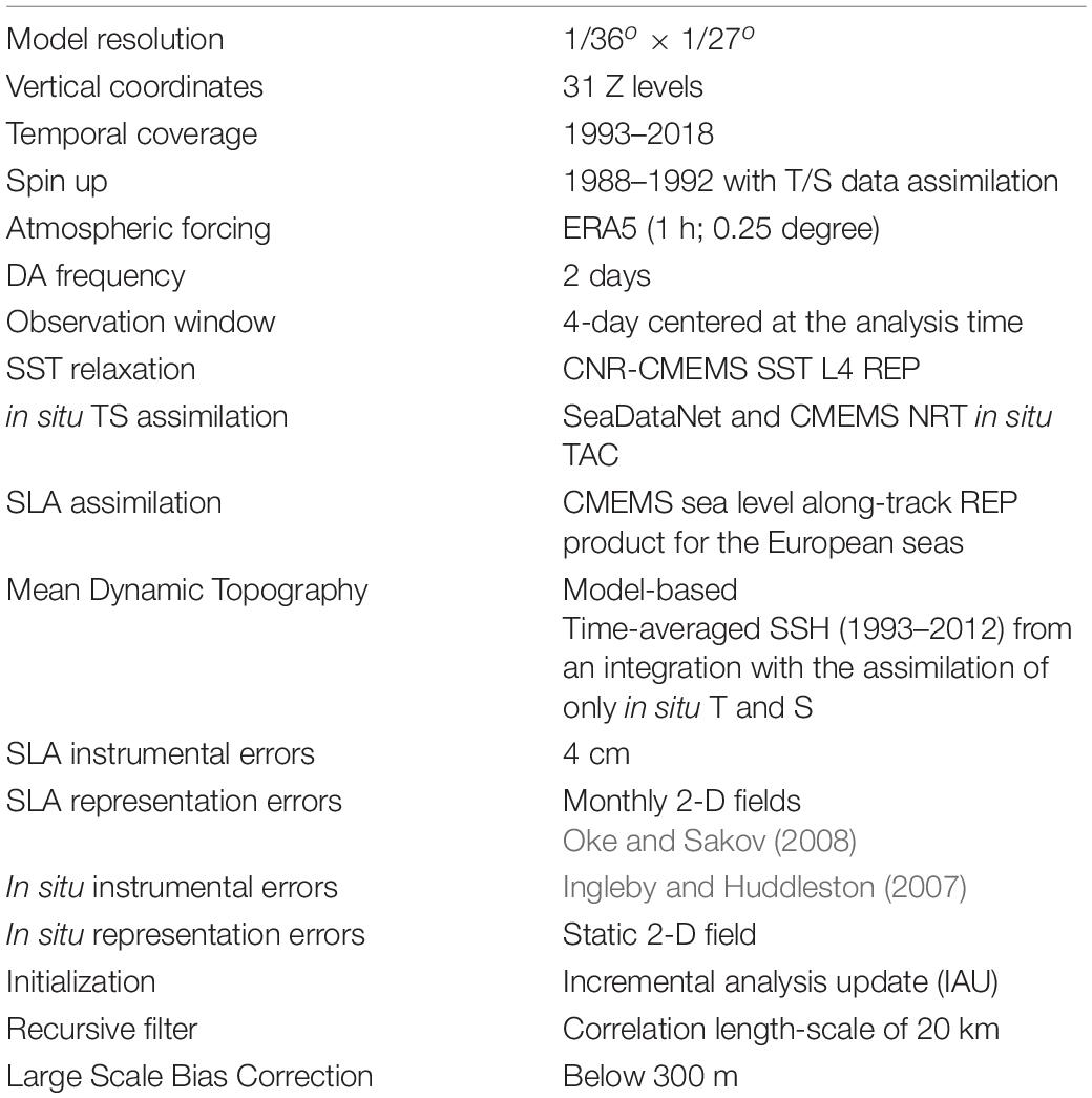
Table 1. BS-REA main configurations.

Results and Discussion

In this section we present the assessment of the BS-REA. Estimated Accuracy Numbers (EAN), which include bias and root mean square difference (RMSD), are computed using the daily outputs of the reanalysis and compared to observations using a quasi-independent approach since the validation is done by comparing the daily-averaged BS-REA fields with respect to both assimilated and rejected observations. Moreover, we provide ocean monitoring indicators such as the temperature, salinity, and ocean heat content anomalies for the Black Sea. Finally, we describe the sea level and upper circulation based on the BS-REA results.

BS-REA Evaluation

In Figure 2, the seasonal maps of the SST bias and RMSD are shown. There is a predominance of positive SST bias all over the basin while a negative bias manifests in limited zones such as the western Anatolian coast in summer and autumn, in river influenced areas in the northwestern shelf during the whole year and in the vicinity of the Azov Sea except in spring. The BS-REA exhibits the lowest RMSD in spring, whereas the highest RMSDs are reached in summer and autumn. For instance, the RMSD exceeds 0.75°C along the upwelling region centered at 33°E (Sur et al., 1994; Özsoy and Ünlüata, 1997) in the Turkish coast, where we believe that overestimated surface winds from the atmospheric dataset may intensify the upwelling events in summer and autumn.

FIGURE 2

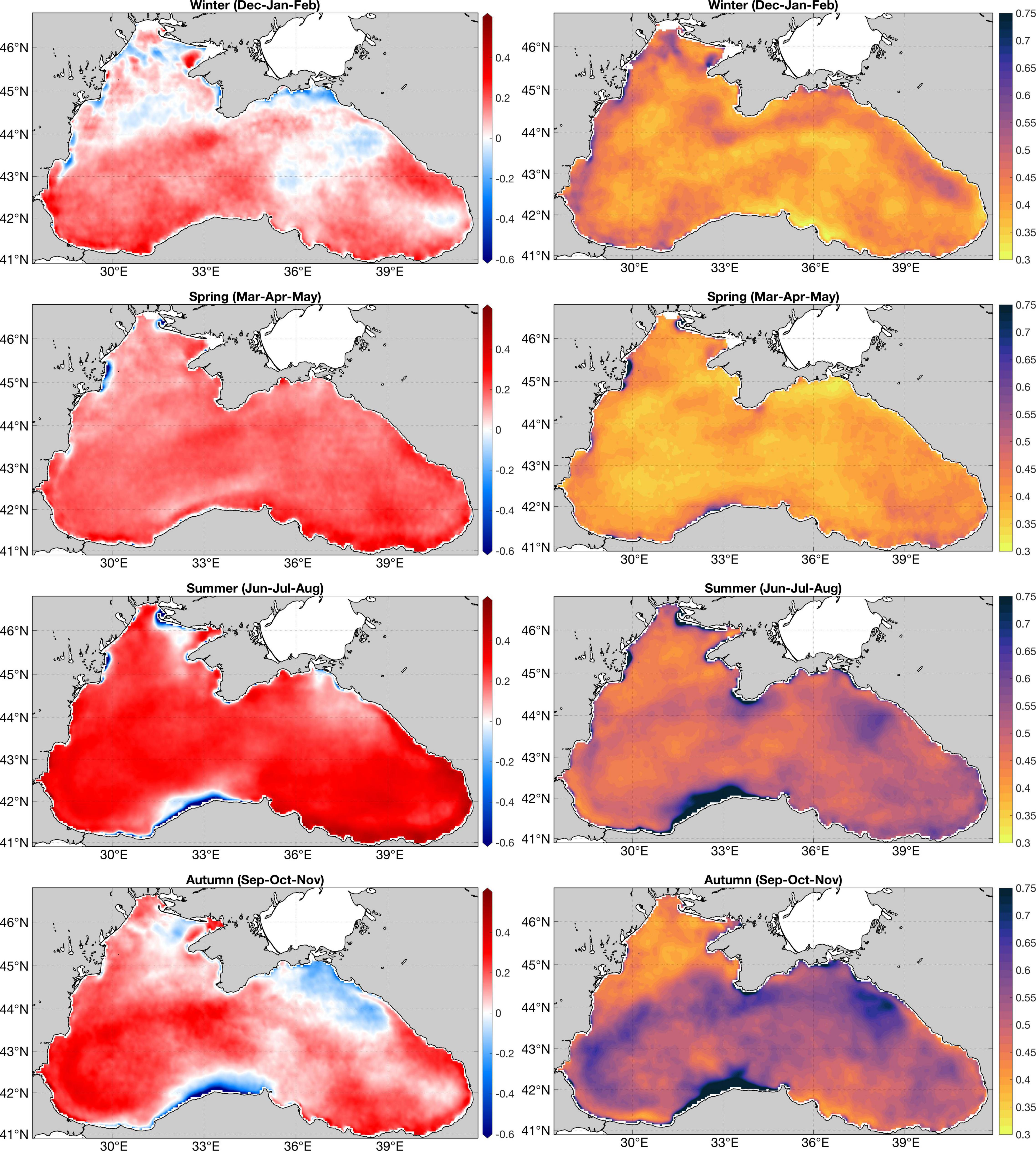
Figure 2. Seasonal maps of the mean bias (left) and RMSD (right) of the SST (^oC) with respect to the satellite SST-L4 products over the period between 1993 and 2018. From top to bottom: winter, spring, summer, and autumn.

In general, BS-REA performs better than the control experiment in terms of bias and RMSD (Table 2). The only variable where it is similar or even slightly lower is the SST which is strongly controlled by the atmospheric forcing and the SST relaxation, both of which are the same in the two experiments. For temperature, the highest RMSDs for the layer 10–100 m are 0.63°C and 1.50°C for BS-REA and the control, respectively. While the control experiment has a negative bias of −0.25°C in the upper layers, BS-REA retains a quite reduced positive bias of 0.01°C.

TABLE 2

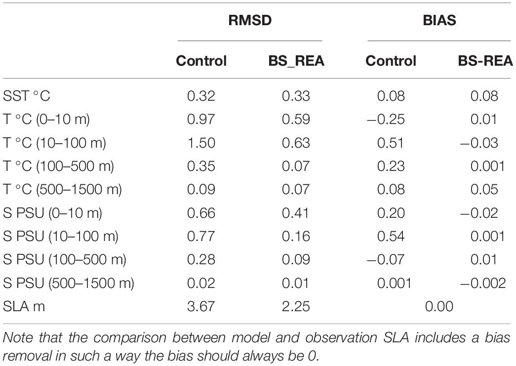
Table 2. EAN estimations for BS-REA and the control experiment without data assimilation.

In Figure 3, we show the vertical temperature error and bias profiles for different subregions in the Black Sea. The RMSD is relatively higher in the northwestern region (dark blue) that is under the influence of the Danube River where a maximum RMSD close to 2.25°C arises around the thermocline. The other two regions with relatively large errors are the northeastern (light blue) and southwestern ones (green), which, respectively, may be related to the absences of the Azov Sea and an open Bosphorus Strait in the BS-REA configuration. Bias profiles manifest the largest discrepancies with the observations above 40 m where there is a predominance of a negative bias (above −0.5°C), except in the northwestern region affected by a positive bias. The Hovmöller diagrams of the temperature bias and RMSD (Figure 4, upper panels) reveal a clear seasonal pattern such that the values are low (high) in winter (summer). The highest errors are in the thermocline, where the prevalence of negative biases is evident each summer from 10 m down to 60 m. There is an evident lack of in-situ observations between 1997 and 2003 in the Black Sea which limits the reanalysis system to be constrained only by altimeter observations for a long time period.

FIGURE 3

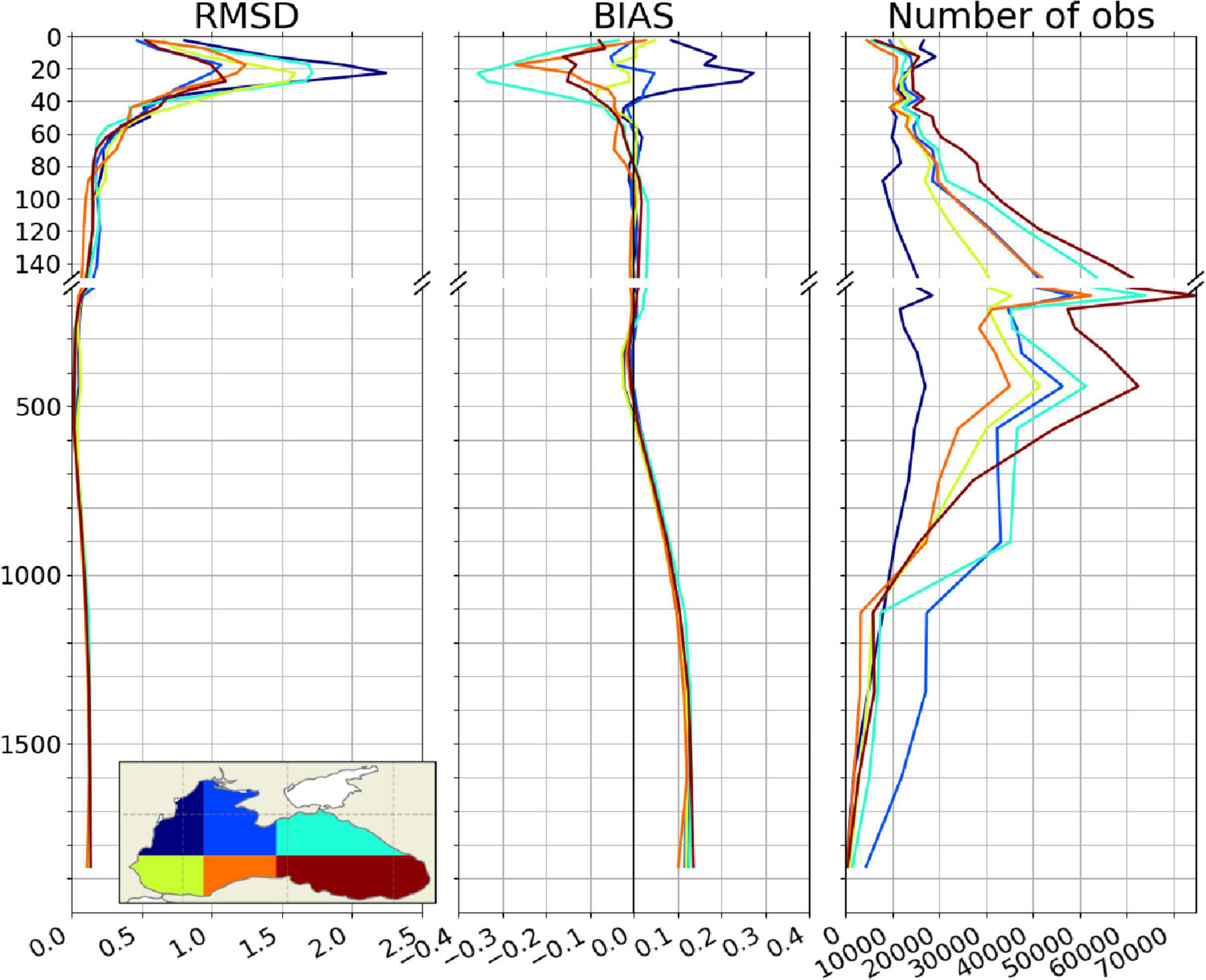
Figure 3. Vertical profiles of the root mean square deviation (left panel), bias (middle panel), and number of observations (right panel) for temperature (°C) for different subdomains in the Black Sea, by comparing the BS-REA results against in situ profilers in the Black Sea domain from 1 January 1993 to 31 December 2018.

FIGURE 4

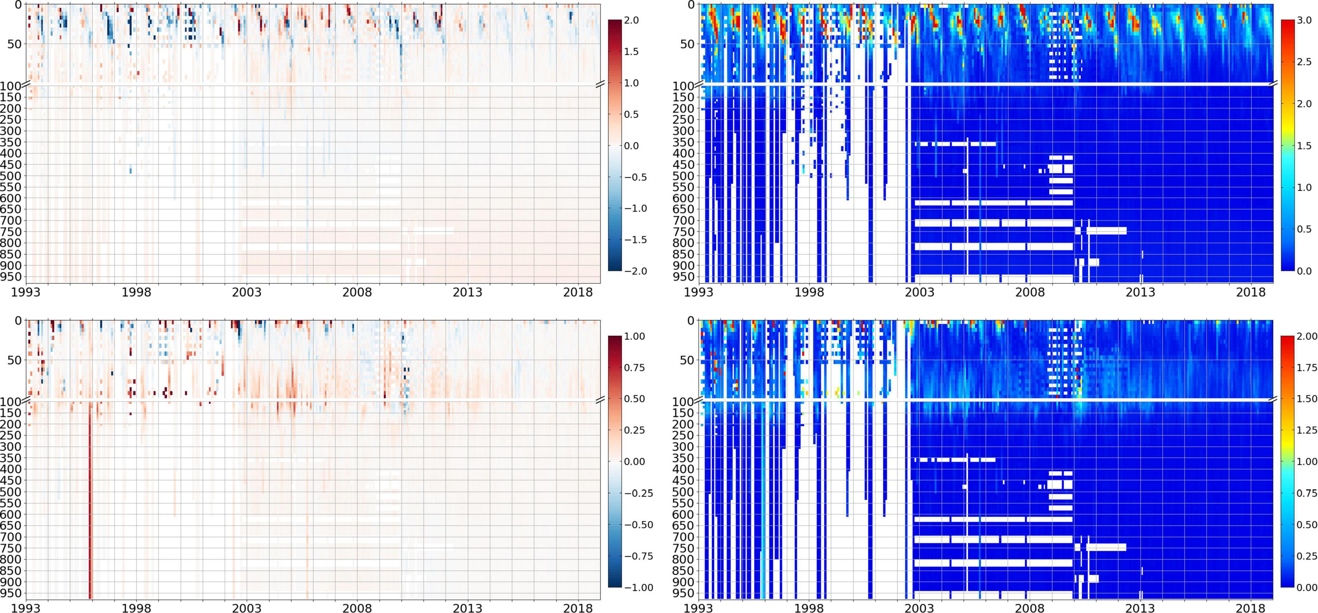
Figure 4. Monthly Hovmöller diagrams of bias (left) and root mean square difference (right) computed against observations of temperature in °C (top) and salinity in PSU (bottom) available in the Black Sea domain from 1 January 1993 to 31 December 2018.

BS-REA shows significant improved skills also for salinity with respect to the control experiment (Table 2). The RMSD is reduced in the entire water column from 0.66 PSU to 0.41 PSU (0.77 PSU to 0.16 PSU) in 0–10 m (10–100 m). The bias is also decreased from surface down to 500 m, mainly in the layer 10–100 m where the BS-REA bias is 0.001 PSU. BS-REA presents a slightly negative bias of −0.02 PSU in 0–10 m.

The vertical error profiles for different regions show that BS-REA represents with less quality the salinity above 20 m, in particular in the northwestern region (Figure 5). In this region, the RMSD overcomes 1.2 PSU at surface and the bias reaches −0.2 PSU at around 10 m depth. This is probably due to the limitation of imposing monthly climatological runoff such as for the Danube River, which may cause a poor representation of salinity close to the river mouth. Unfortunately, we do not have a long and uninterrupted time series of river discharges for the Black Sea to be used for a more accurate parameterization. In deeper levels, the salinity RMSD is relatively higher only in the southwestern region in the layer 60–100 m where the RMSD exceeds 0.4 PSU. This may be due to the parameterization of the Bosphorus Strait in the current model configuration in which we relax the model towards a climatology from a model simulation. Nevertheless, bias is low in the southwestern Black Sea and comparable to other regions. Hovmöller diagrams show that both salinity bias and RMSD remain low over time (Figure 4, bottom panels). However, we note large RMSD that may exceed 1.5 PSU near the surface, mainly during some temporal intervals before 2008.

FIGURE 5

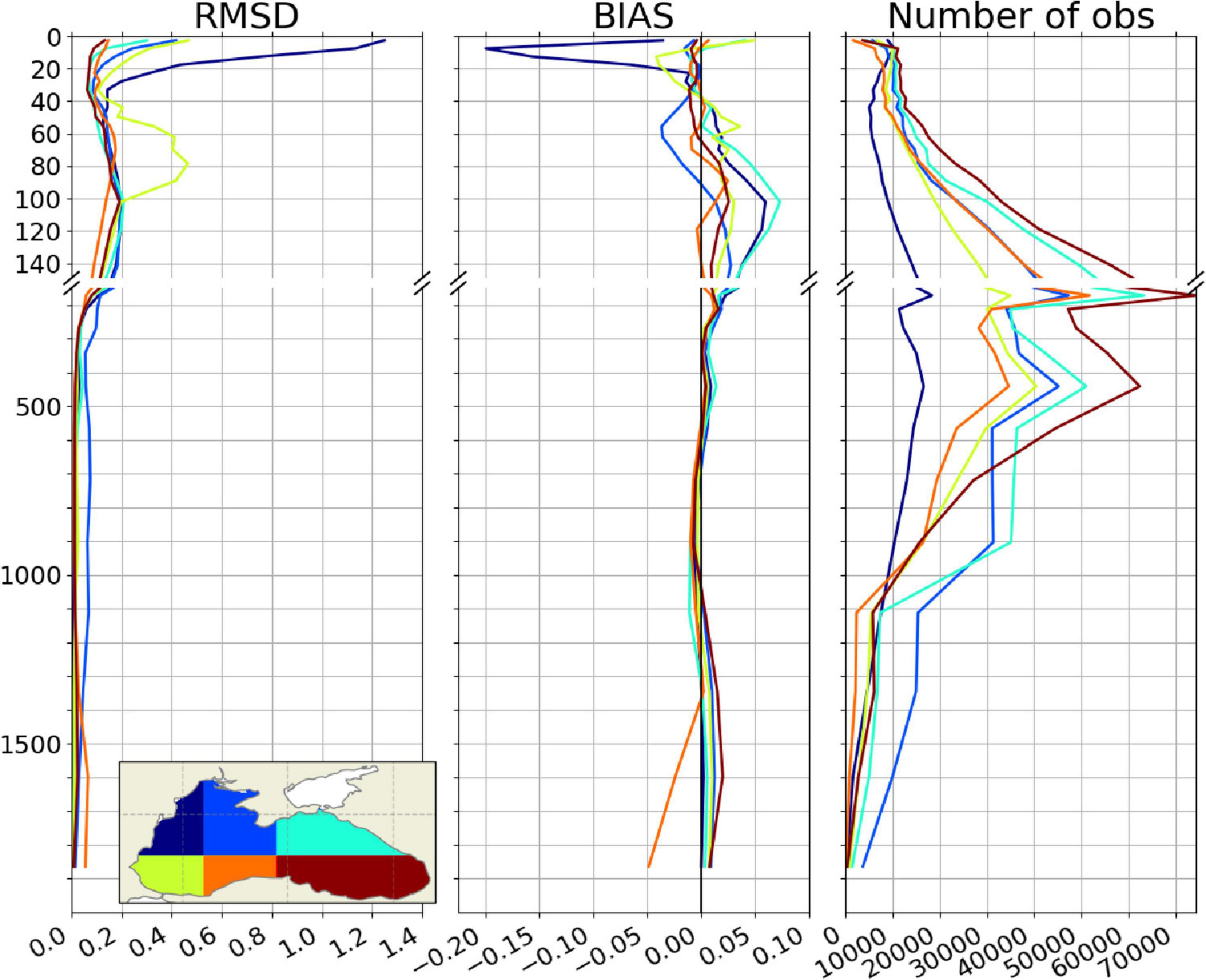
Figure 5. Vertical profiles of the root mean square deviation (left panel), bias (middle panel) and number of observations (right panel) for salinity (PSU) for different sub-domains in the Black Sea, by comparing the BS-REA results against in situ profilers in the Black Sea domain from 1 January 1993 to 31 December 2018.

The mean RMSD of sea level anomaly is 2.25 cm for BS-REA which corresponds to a reduction of ∼39% with respect to the control (Table 2). Time series of SLA RMSD present a continuous reduction of the values during the first years of BS-REA integration. Error values fluctuate around 2 cm since 2005, whereas the control error ranges between 3 and 4 cm, sometimes exceeding 4 cm (Figure 6). Horizontal maps of RMSD reveal minor seasonal differences with the largest values close to the shelf areas (not shown), where there is a dominance of the mesoscale activities along the Rim Current. For example, relatively high errors can be found in the Crimean Peninsula, where there is a regular activity of the Sevastopol eddy, and in the southeastern region, which is related to the presence of the Batumi eddy. These eddies are quasi-stationary anticyclonic features that have been examined in the Black Sea (Kubryakov and Stanichny, 2015; Kubryakov et al., 2018).

FIGURE 6

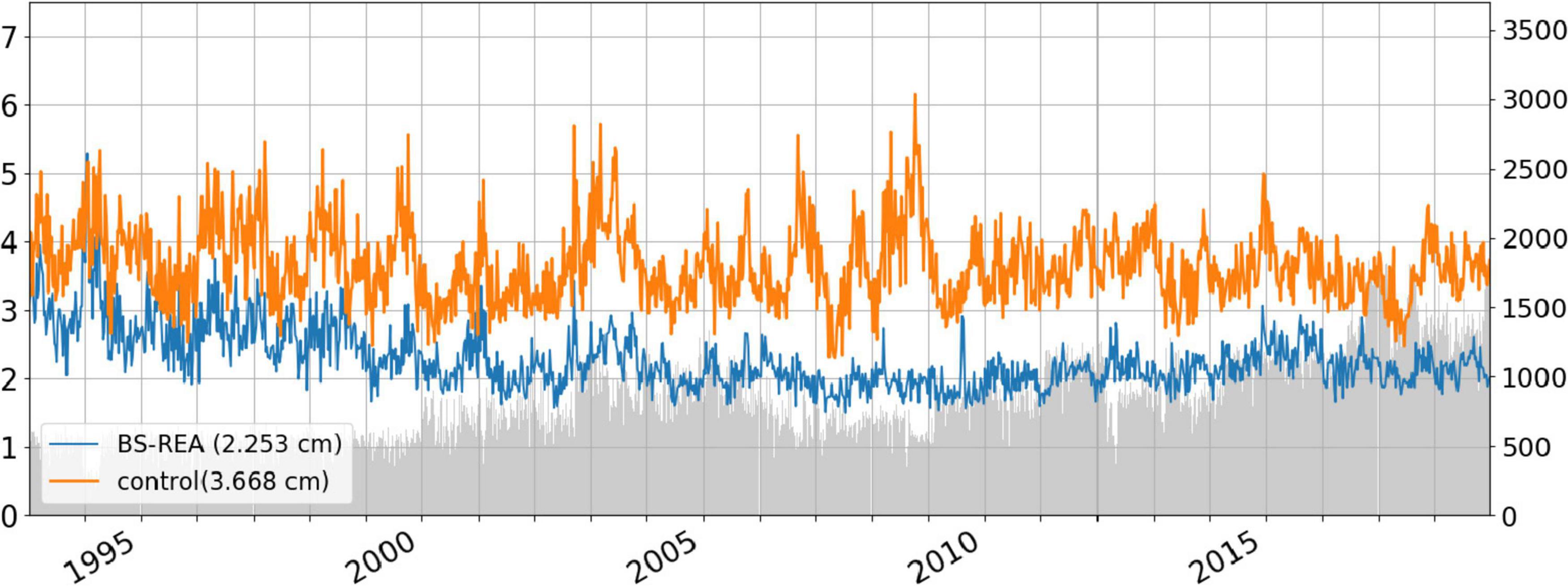
Figure 6. Time series of sea level anomaly RMSD by considering the results of BS-REA (blue) and control experiment (orange) against sea level anomaly along-track observations in the Black Sea domain. The shaded area and the right axis correspond to the number of observations.

Temperature and Salinity Trends

This section examines the time variability of temperature and salinity as well as their trends for the whole BS-REA period (1993–2018) and its latest 14 years (2005–2018).

Initially, the basin-averaged temperature time series shown in Figure 7 demonstrate a high seasonal variability in 0–25 m, with values above (below) 20°C (7.5°C) in most of the summers (winters). The seasonal signal weakens between 25 and 150 m and disappears below 150 m. The temperature trends are estimated in two different periods (1993–2018 and 2005–2018) and indicate an overall warming of the basin especially in the period 2005–2018 with a decreasing trend in deeper layers. The values are 0.083°C year^–1 (0.12°C year^–1) in 0–25 m and reduce to 0.0041°C year^–1 (0.0092°C year^–1) in 150–300 m for the period 1993–2018 (2005–2018). For comparison, Ginzburg et al. (2004) used satellite measurements to reveal a positive trend of 0.09°C year^–1 in sea surface temperature over the years 1982–2000. Miladinova et al. (2017) did not detect a significant trend in the SST from model simulations considering the period 1960–2015, whereas the temperature at 200 m indicated a positive trend of 0.005°C year^–1. BS-REA warming is more noticeable starting from 2005, especially in the 150–300 m layer, where instead a negative trend between 1993 and 2001 is reproduced by the reanalysis. BS-REA also presents a continuous warming in the layer 25–150 m, where the Black Sea CIL resides. In response, the CIL almost disappeared in recent years as is discussed in the next paragraph. Stanev et al. (2019) reached a similar result using observations.

FIGURE 7

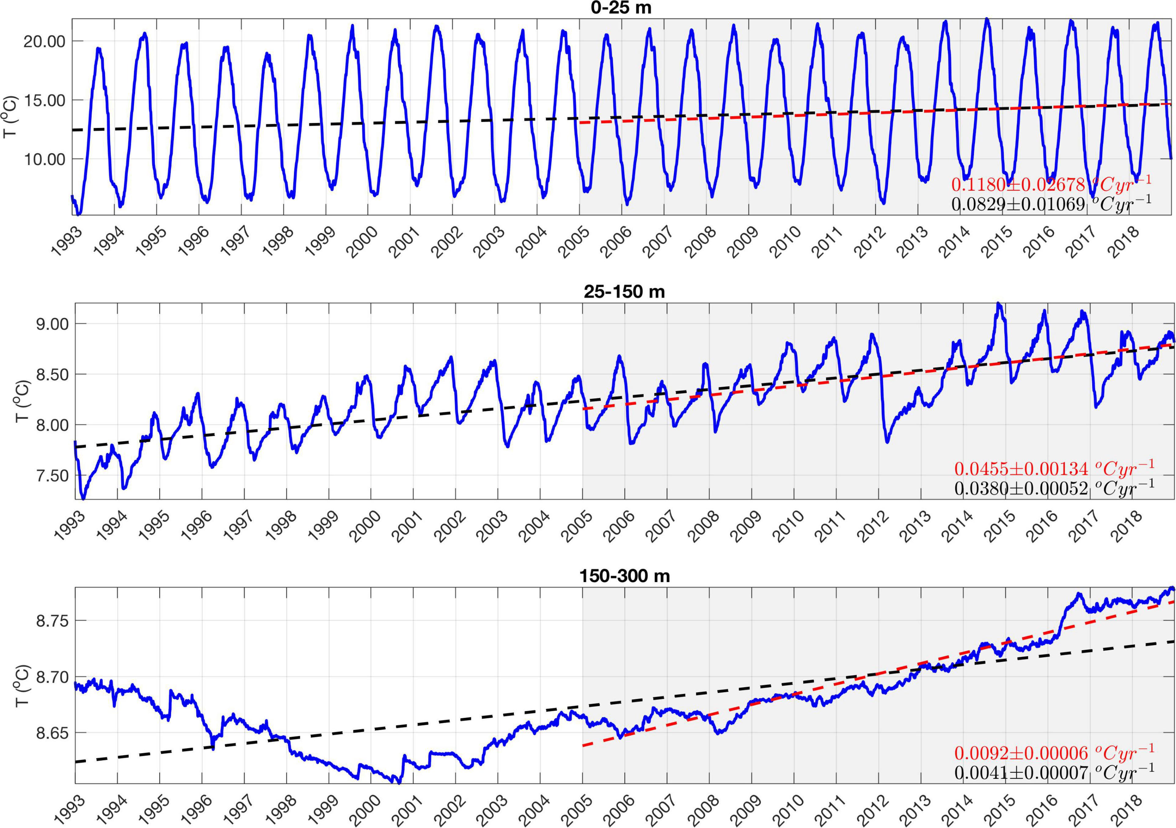
Figure 7. Time evolution of the basin-averaged temperature in °C computed from BS-REA in different layers: 0—25 m (top), 25–150 m (central), and 150–300 m (bottom). The dashed lines are the linear trends for the period 1993–2018 (black) and 2005–2018 (red), mean trend values are also reported in the figures (bottom right corner).

Figure 8 (top left panel) shows the time evolution of basin mean temperature and the 8°C isotherm is chosen to track the Black Sea CIL over time. The CIL formation is related to the water cooling during the winter season and its presence is evident continuously until 2008. From 1993 to 2000, the CIL resides from surface down to ∼100 m. There is a weakening of the CIL in 2001 when the temperature exceeds 8°C in most of the water column. The CIL forms again in 2002 but not as strong as in the previous years so that the 8°C isotherm occupies depths above 75 m. The pattern completely changes after 2008, when the temperatures clearly increase in such a way that the CIL disappears most of the time. Between 25 and 150 m the temperature increase (shown in Figure 7) reflects a trend value of 0.045°C year^–1 for the period 2005–2018, by revealing a faster warming of the Black Sea over recent years. Degtyarev (2000) also noted a positive temperature trend of 0.016°C years^–1 in a less thick layer (50–100 m) from 1985 to 1997. After 2008, the formation and presence of the CIL is observed only in 2012 and, to a lesser extent, in 2017. Figure 8 (bottom left panel) shows the basin mean temperature anomaly with respect to a reference climatology evaluated from the same reanalysis in the period 1993–2014. The temperature anomaly is mostly negative before 1999, while during the period 1999–2008, it shows a clear annual variability in the upper 250 m, fluctuating between negative and positive values around the reference baseline. Since 2009, there is a predominance of positive anomalies so that values exceed 1.5 °C at upper layers, which again supports the Black Sea warming and disappearance of the CIL during recent years. Reports based on previous versions of BS-REA also found a surface warming and an increase in the ocean heat content of the Black Sea in the past few years (Mulet et al., 2018; Lima et al., 2020c) which will be discussed in section 3.3.

FIGURE 8

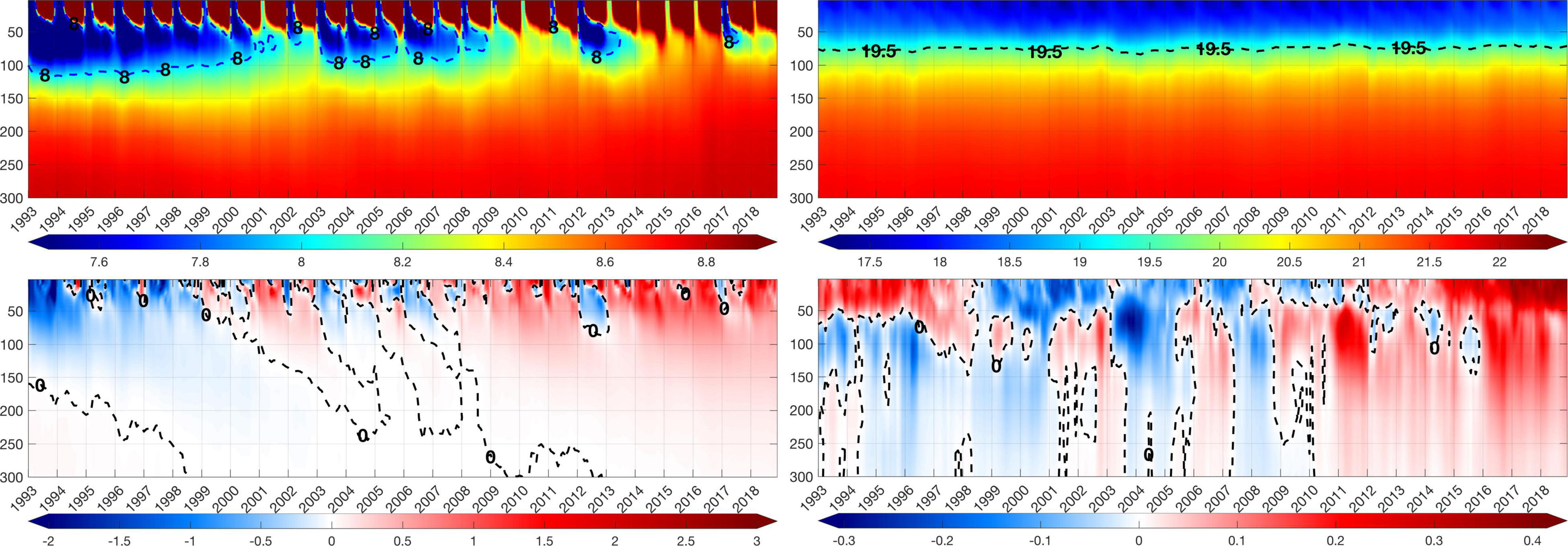
Figure 8. Time versus depth diagrams of the monthly basin-averaged temperature in °C (top left), anomaly of temperature in °C (bottom left), monthly basin-averaged salinity in PSU (top right), and anomaly of salinity in PSU (bottom right). The monthly anomaly estimates considered the climatological period 1993–2014 of each corresponding month. The blue dashed line indicates the mean position of the 8°C isotherm (top left), whereas the dashed black line represents the isoline of 19.5 PSU (top right) and null anomaly (bottom panels).

In Figure 9, similar analyses for salinity reveal that salinity trends reduce in depth and are higher during the most recent period (2005–2018) especially in surface layers. Trends are 0.0068 PSU year^–1 (0.0359 PSU year^–1) in 0–25 m, decrease to 0.0062 PSU year^–1 (0.0131 PSU year^–1) in 25–100 m and finally to 0.0029 PSU year^–1 (0.005 PSU year^–1) in 150–300 m during the period 1993–2018 (2005–2018). For comparison, Miladinova et al. (2017) identified different salinity trends at the surface (negative), upper (weaker negative) and main halocline (positive) for the period 1960–2015. The time evolution of salinity shows well-defined layers, such that mean values are less than 18.5 PSU above 50 m, reach 20–20.5 PSU at 100 m and exceed 21.5 PSU in deeper waters down to 300 m (Figure 8; top right panel). Above 50 m, salinity anomalies, evaluated with respect to a reference climatology from the same reanalysis in the period 1993–2014 exhibit periods that alternates with the predominance of positive and negative anomalies: anomalies are positive until the beginning of 1998, mostly negative from 1998 to 2011, and again positive starting from 2012 (Figure 8; bottom right panel). A notable characteristic is the presence of larger positive anomalies from 2016, which indicates a recent salinization in the sea. In 50–100 m, large negative anomalies are present in 2004–2005, whereas maximum positive anomalies are seen in 2011. After 2016, salinity anomalies are only positive.

FIGURE 9

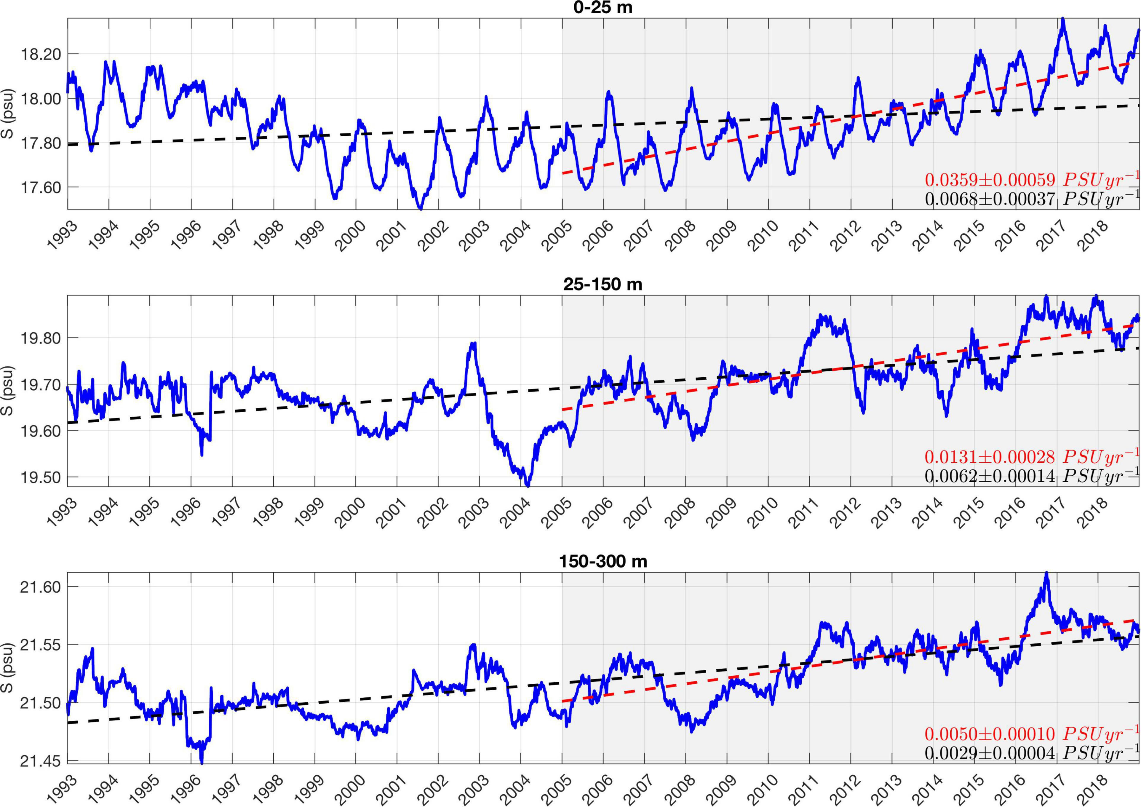
Figure 9. Time evolution of the basin-averaged salinity in PSU computed from BS-REA in different layers: 0–25 m (top), 25–150 m (central), and 150–300 m (bottom). The dashed lines are the linear trends for the period 1993–2018 (black) and 2005–2018 (red), mean trend values are also reported in the figures (bottom right corner).

Ocean Heat Content

The investigation of the Black Sea ocean heat content follows Lima et al. (2020c), who defined the ocean heat content like anomalies with respect to the reference period of 2005–2014, following the equation below:

$$OHC={\int }_{z_1}^{z_2}{\mathrm{\rho }}_0{c}_p\left(T_m-T_{clim}\right)\mathit{d}z(7)$$

with ρ₀ equal to 1020 kg m^–3 and c_p equal to 4181.3 J kg^–1°C ^–1 are, respectively, the density and specific heat capacity; and dz indicate the a certain ocean layer limited by the depths z₁ and z₂; T_m corresponds to the monthly average temperature and T_climis the climatological temperature of the corresponding month.

In this study the ocean heat content is estimated as the deviation from the reference period of 1993–2014. A clear positive trend of 0.11 W m^–2 characterizes the 0–10 m layer (Figure 10). Above this trend, warm peaks appear in the second half of the year 1994, less intense in 1996 and increased again in 2010 and 2012. The highest positive peak occurs in the 2018 autumn. As thicker layers are considered, the trends increase, whereas time series present a lower variability over time; for the period 1993–2018, trends are 0.45 W m^–2, 0.81 W m^–2 and 0.83 W m^–2, respectively, in 0–50, 0–200, and 0–1000 m. For comparison, trends are also estimated for the period 2005–2018 and reveal higher values down to 200 m as compared to Lima et al. (2020c) (Table 3), which may be related to the different period (2005–2014) that they used to estimate the reference climatology. Considering thicker layers, it becomes clear that an increase in ocean heat content weakens the CIL like in 2001, whereas its decreasing favors the CIL restoration like in the years 2012 and 2017, as is viewed in Figure 8 (top left panel). In 2012, times series for 0–10 m exhibits colder waters already in 2011 that appear in 2012 only when layers as thick as 50 m are considered, which indicates that colder waters moved from surface in 2011 to generate the CIL in 2012 (Figure 10). A migration of colder and saltier water from surface to deeper layers also produced a signature in the temperature and salinity anomalies (Figure 8; bottom panels). A less intense CIL formation occurred in 2017 and again a water cooling in the 0–10 m layer is evident in the previous year, 2016.

FIGURE 10

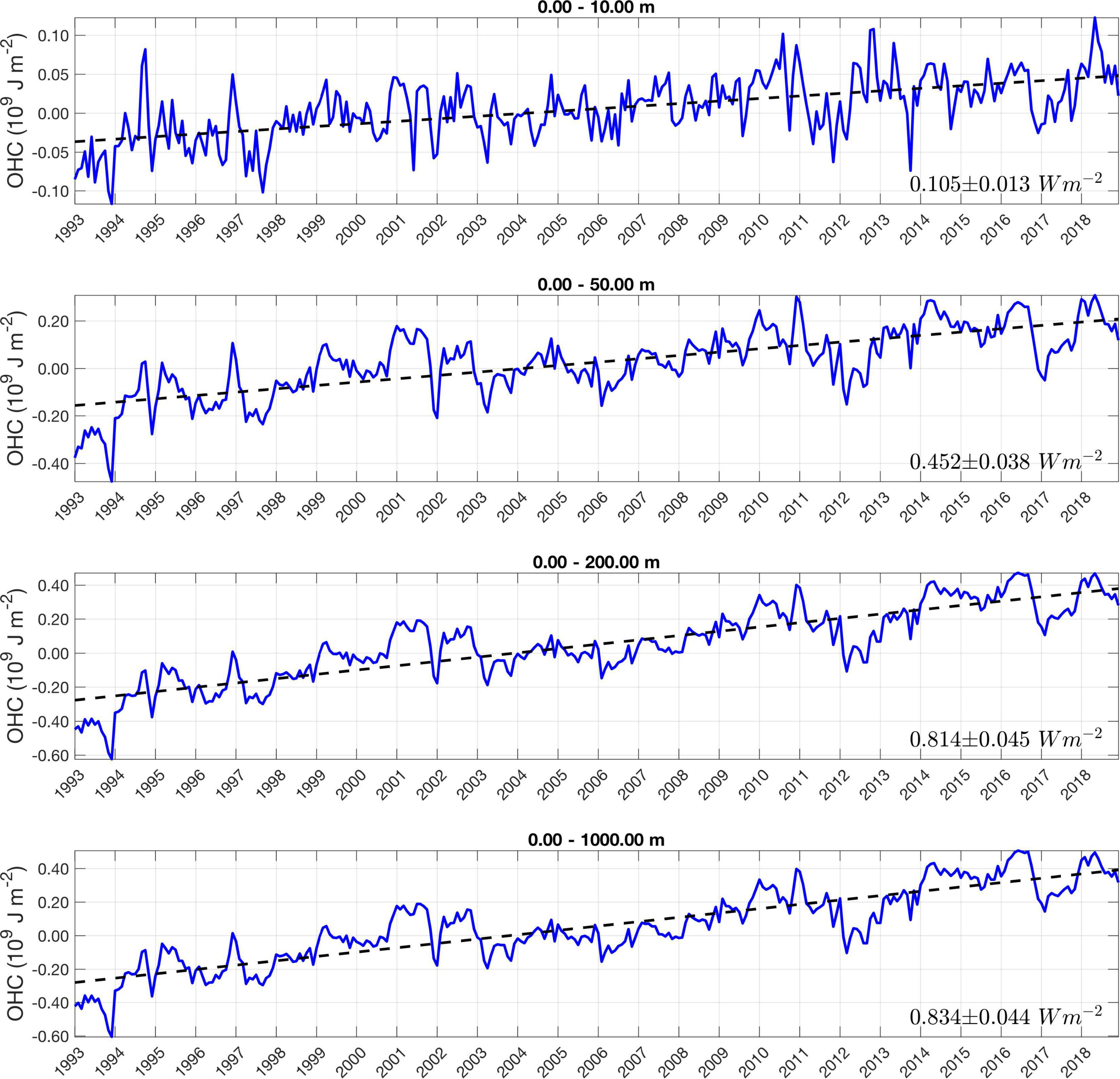
Figure 10. Monthly basin-averaged of the ocean heat content anomalies (in 10⁹ J m^–2) estimated for the BS-REA. The monthly ocean heat content anomalies are defined as the deviation from the climatological ocean heat content mean (1993–2014) of each corresponding month. Mean trend values are also reported in the figures (bottom right corner).

TABLE 3

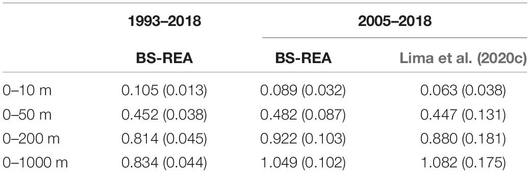
Table 3. Trends estimations together with the 95% confidence interval (in brackets) for the ocean heat content anomaly (W m^–2) from BS-REA and Lima et al. (2020c) for the period 1993–2018 and 2005–2018.

Spatial maps of yearly depth-integrated ocean heat content anomalies (0–200 m) show a predominance of negative values from 1993 until 1998 (Figure 11). Lowest values are found in 1993 at the margins of the basin. In 1999, positive values appear mostly in shallow regions at the basin borders, but also in deeper regions like along the Rim Current pathway near the Crimean Peninsula. In this region, positive values may be associated with the presence of the Sevastopol eddy, a quasi-stationary anticyclonic eddy located close to the Crimean Peninsula. The pattern changes completely in 2001 and 2002, when the ocean heat anomaly assumes positive values in a large part of the basin, which brings a weakening of the Black Sea CIL in these years (see also Figure 8; top left panel). In the period from 2003 to 2006, there is again a predominance of negative values, except in 2004, when a prevalence of positive values is viewed in the central region. Since 2007, the warming signal is very clear in such a way that the ocean heat content anomalies achieve the highest positive values near the Crimean Peninsula in 2010, near the Bulgarian and Turkish coasts in 2016 and in the southeastern region in 2013, 2015 and 2018. However, this continuous warming is interrupted in 2012 and less explicitly in 2017, years in which a replenishment of the CIL is verified, as is also shown in Figure 8.

FIGURE 11

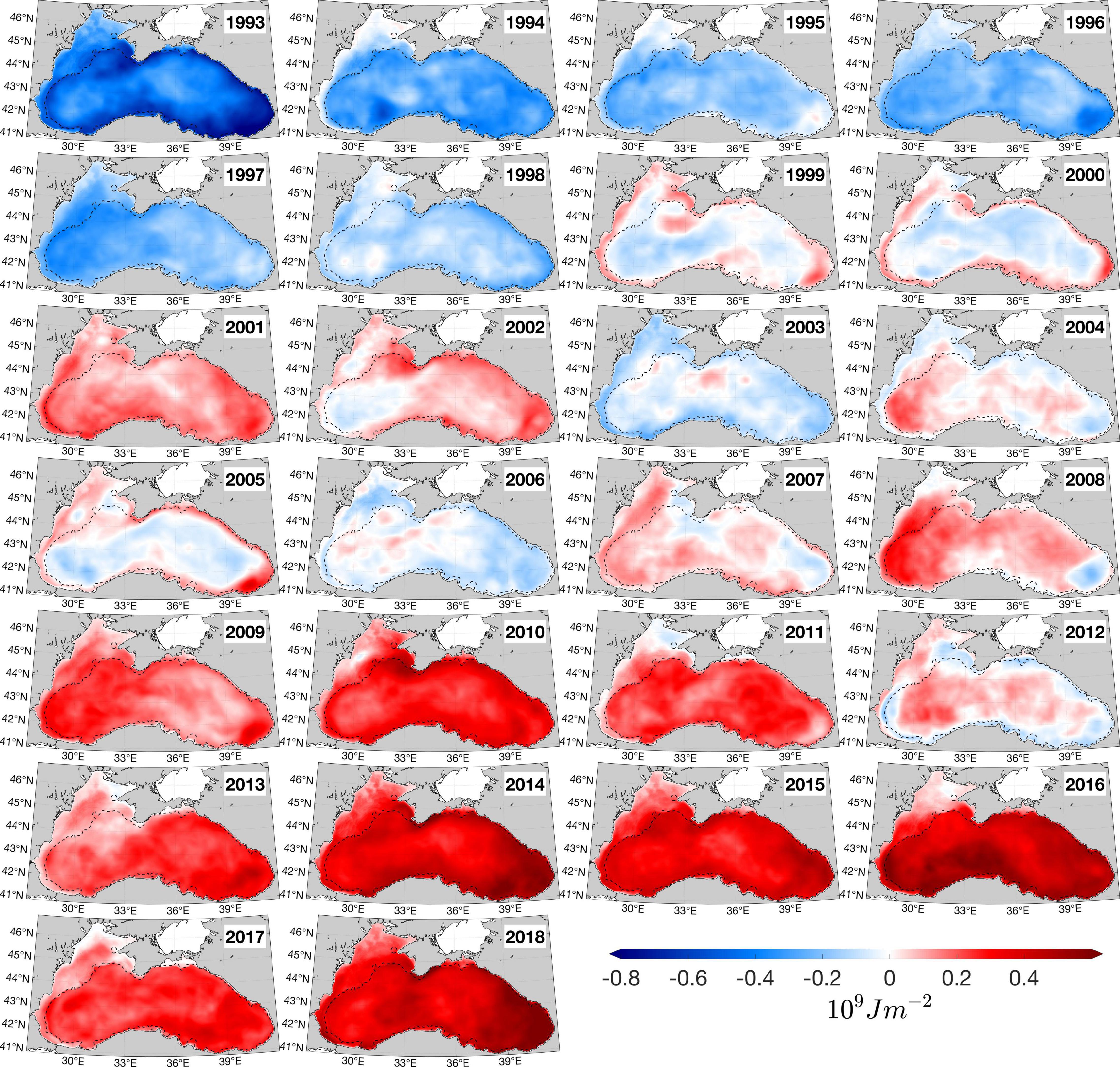
Figure 11. Yearly depth-integrated (0-200 m) ocean heat content anomalies (in 10⁹ J m^–2) estimated for the BS-REA and defined as the deviation from the reference period of 1993–2014. Black isoline indicates the 200 m isobath.

Surface Topography and Upper Layer Circulation

Figure 12 shows annual and seasonal mean sea surface height (SSH) fields overlaid by the upper 100 m depth-averaged velocity. The mean SSH varies spatially, i.e., low values dominate the inner basin while the shelf and coastal zones have high values. Similar formation persists when the signal is decomposed into its seasonal components. In winter and spring, the negative values of SSH extend to the easternmost coast. In summer and autumn, the western basin presents similar SSH properties while, in the eastern basin, the negative values are more restricted to the inner basin.

FIGURE 12

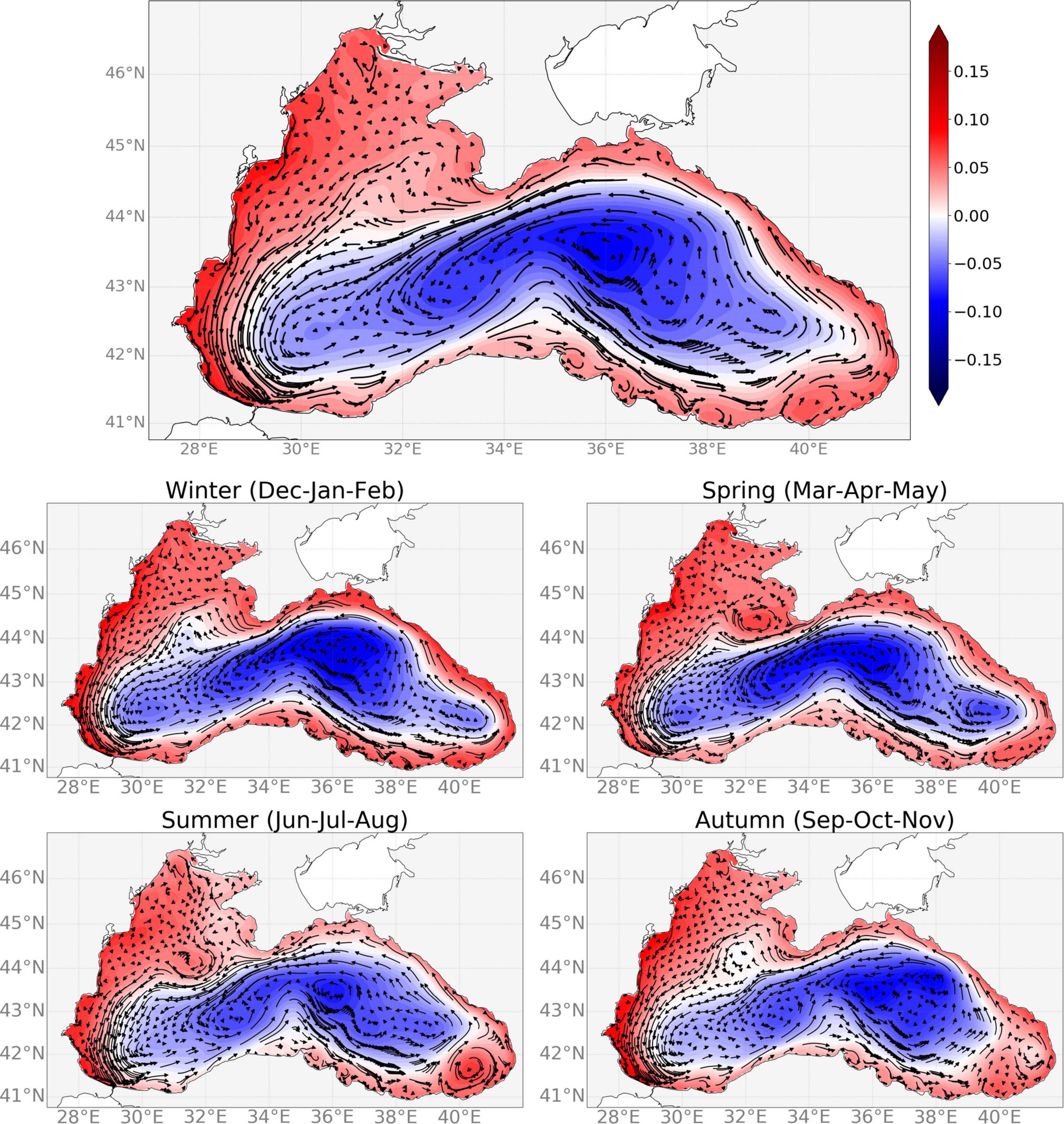
Figure 12. Mean sea surface height and 100 m depth average velocity derived from the BS-REA evaluated for the whole period 1993-2018 (top panel) and each season considering the climatological period 1993–2018.

The upper layer Black Sea circulation structures are consistent with the SSH gradients showing a seasonal variability with the only exception of the permanent Rim Current encircling the entire basin and forming a large-scale cyclonic gyre. The mean upper layer circulation develops around the Rim current together with the Batumi gyre in the easternmost basin and smaller scale eddies along the Anatolian coast. The Rim current bifurcates into two branches after the Crimean Peninsula with a smaller one recirculating in the northwestern shelf and merges back to the main branch around 30.5°E. The Rim current accelerates along the Turkish coast around 32°E, then detaches from the shelf and penetrates into the deep basin before going again close to the coast around 35.5°E. In winter, the eastern and western gyres are less defined. Following the Rim Current, the Batumi anticyclonic eddy is well defined in summer, seems to be more confined near the Georgia coast in autumn, but it is less apparent in winter and spring. Next, the presence of Sevastopol anticyclonic eddy is very clear near the southwest of the Crimean Peninsula in spring and summer, whereas it is less distinguishable in winter and autumn. All these circulation patterns are consistent with the previous estimates described in Oguz et al. (1993); Özsoy and Ünlüata (1997), Korotaev et al. (2003) and Gunduz et al. (2020).

Conclusion

The BS-REA system shows very satisfactory skills compared to the model simulation, which highlights the importance of using data assimilation to improve the model representation. BS-REA also has the ability to represent the main Black Sea circulation, the Rim Current, as well as the mesoscale features in the Black Sea, such as the quasi-stationary anticyclones Sevastopol and Batumi eddies, respectively, near the Crimean Peninsula and southeastern region. Notwithstanding, the BS-REA has shown a reduced ability to represent the impact of Danube waters on the sea, which is possibly due to the current model configuration such as the application of monthly climatological runoff. Furthermore, the absence of the Bosphorus and Kerch straits negatively impacts the BS-REA representation in regions adjacent to the Azov and Marmara Seas.

The system is very suitable for understanding the physical state of the Black Sea in recent years and allows to obtain more accurate ocean monitoring indicators for the sea, which are important to understand its response to climate change. The temperature analyses have indicated a recent faster warming of the Black Sea that has impacted its CIL formation. Since 2009, the disappearance of CIL is evident, although some weaker CIL sporadic events are detected in 2012 and 2017. Additional investigations show a relative reduction in the ocean heat content in these years, which coincides with the reemergence of the CIL.

Trends in temperature, salinity and ocean heat content reveal a warming and salinification of the Black Sea, especially in the past few years. However, since trends based on short records are very sensitive to the beginning and end values of the time series and cannot in general reflect long-term climate trends, longer time series are needed to confirm these tendencies. This requires a continuous improvement of the BS-REA system through new developments in ocean modeling and data assimilation together with the maintenance of the Black Sea ocean observation system. In addition, for future work, we consider comparing our results with global models such as those from the Ocean Model Intercomparison Project (Lin et al., 2020; Chassignet et al., 2020) and global ocean reanalyses (Storto et al., 2019a, b), which can also allow us to quantify uncertainties through an ensemble of model results in the Black Sea.

In order to further improve the reanalysis, the next generation of the Black Sea systems will include a revision of the hydrodynamical core and new capacities from the data assimilation scheme. Regarding the core model, the new version will use higher resolution in vertical (e.g., from 31 to 121 z-levels with partial steps) and upgrade to NEMO v4.0. The Bosphorus Strait is going to be represented as an open boundary thanks to the inclusion of the Marmara Sea box in the numerical grid: it will ingest the high-resolution model solutions provided by the Unstructured Turkish Straits System (U-TSS, Ilicak et al., 2021) - T, S, SSH, U, V - with the scope to optimally interface the Black Sea with the Mediterranean Sea. Such new developments, together with the revision of the land forcing and data assimilation scheme to account for high resolution EOF, will be part of the new Black Sea forecasting system (Ciliberti et al., 2021) that entered in service in May 2021 and will be uptaken by the BS-REA in the near future.

Data Availability Statement

The datasets presented in this study can be found in online repositories. The names of the repository/repositories and accession number(s) can be found below: https://doi.org/10.25423/CMCC/BLKSEA_MULTIYEAR_PHY_007_004.

Author Contributions

LL led the work, developed the reanalysis system, and contributed to the elaboration of this work at all levels. SCi led the hydrodynamical model development and provided a valuable scientific contribution to improve this work at different levels. DA, SCa, and MI contributed to the hydrodynamical model development. SM contributed to the scientific scope, providing important insights to improve this work at different levels. AA contributed to improving the model setup, particularly for the correction of the model freshwater budget and provided a valuable scientific contribution to improve this work at different levels. RE contributed to define the validation strategy. AC contributed to set up the bias correction scheme. AA, RE, AC, and EJ contributed to define the data assimilation strategies. RL provided the access to all available observational dataset. SCr, LS, and FP contributed to set up the operational procedures and interfaces. EP, GC, and EC provided useful comments that helped to guide this work. All authors contributed to the article and approved the submitted version.

Funding

This research was funded by the Copernicus Marine Environment and Monitoring Service for the Black Sea Monitoring and Forecasting Centre (Contract No. 72-CMEMS-MFC-BS).

Conflict of Interest

The authors declare that the research was conducted in the absence of any commercial or financial relationships that could be construed as a potential conflict of interest.

Publisher’s Note

All claims expressed in this article are solely those of the authors and do not necessarily represent those of their affiliated organizations, or those of the publisher, the editors and the reviewers. Any product that may be evaluated in this article, or claim that may be made by its manufacturer, is not guaranteed or endorsed by the publisher.

Footnotes

1. ^ https://www.gebco.net/
2. ^ https://www.ngs.noaa.gov/CUSP
3. ^ http://www.seadatanet.org

References

Adler, R. F., Huffman, G. J., Chang, A., Ferraro, R., Xie, P. P., Janowiak, J., et al. (2003). The version-2 global precipitation climatology project (GPCP) monthly precipitation analysis (1979-present). J. Hydrometeor. 4, 1147–1167. doi: 10.1175/1525-7541(2003)004<1147:tvgpcp>2.0.co;2

CrossRef Full Text | Google Scholar

Akpinar, A., Fach, B. A., and Oguz, T. (2017). Observing the subsurface thermal signature of the Black Sea cold intermediate layer with Argo profiling floats. Deep Sea Res. I Oceanogr. Res. Papers 124, 140–152. doi: 10.1016/j.dsr.2017.04.002

CrossRef Full Text | Google Scholar

Aydoğdu, A., Pinardi, N., Özsoy, E., Danabasoglu, G., Gürses, Ö., and Karspeck, A. (2018). Circulation of the Turkish straits system under interannual atmospheric forcing. Ocean Sci. 14, 999–1019. doi: 10.5194/os-14-999-2018

CrossRef Full Text | Google Scholar

Balmaseda, M. A. (2017). Data assimilation for initialization of seasonal forecasts. J. Mar. Res. 75, 331–359. doi: 10.1357/002224017821836806

CrossRef Full Text | Google Scholar

Bloom, S. C., Takacs, L. L., Silva, A. M. D., and Ledvina, D. (1996). Data assimilation using incremental analysis updates. Mon. Wea. Rev. 124, 1256–1271. doi: 10.1175/1520-0493(1996)124<1256:dauiau>2.0.co;2

CrossRef Full Text | Google Scholar

Buongiorno Nardelli, B., Tronconi, C., Pisano, A., and Santoleri, R. (2013). High and ultra-high resolution processing of satellite sea surface temperature data over Southern European seas in the framework of MyOcean project. Rem. Sens. Environ. 129, 1–16. doi: 10.1016/j.rse.2012.10.012

CrossRef Full Text | Google Scholar

Castellari, S., Pinardi, N., and Leaman, K. (1998). A model study of air-sea interactions in the Mediterranean Sea. J. Mar. Sys. 18, 89–114. doi: 10.1016/s0924-7963(98)90007-0

CrossRef Full Text | Google Scholar

Chassignet, E. P., Yeager, S. G., Fox-Kemper, B., Bozec, A., Castruccio, F., Danabasoglu, G., et al. (2020). Impact of horizontal resolution on global ocean–sea ice model simulations based on the experimental protocols of the Ocean Model Intercomparison Project phase 2 (OMIP-2). Geosci. Model Dev. 13, 4595–4637. doi: 10.5194/gmd-13-4595-2020

CrossRef Full Text | Google Scholar

Ciliberti, S. A., Jansen, E., Martins, D., Gunduz, M., Ilicak, M., Stefanizzi, L., et al. (2021). Black Sea Physical Analysis and Forecast (CMEMS BS-Currents, EAS4 system) (Version 1) [Data set]. Copernicus Monitoring Environment Marine Service (CMEMS). doi: 10.25423/CMCC/BLKSEA_ANALYSISFORECAST_PHY_007_001_EAS4

CrossRef Full Text | Google Scholar

Ciliberti, S. A., Peneva, E. L., Jansen, E., Martins, D., Cretí, S., Stefanizzi, L., et al. (2020). Black Sea Analysis and Forecast (CMEMS BS-Currents, EAS3 system) (Version 1) [Data set]. Copernicus Monitoring Environment Marine Service (CMEMS). doi: 10.25423/CMCC/BLKSEA_ANALYSIS_FORECAST_PHYS_007_001_EAS3

CrossRef Full Text | Google Scholar

Courtier, P. (1997). Variational methods. J. Meteor. Soc. Japan 75, 211–218.

Google Scholar

de Souza, J. M. A. C., Couto, P., Soutelino, R., and Roughan, M. (2020). Evaluation of four global ocean reanalysis products for New Zealand waters–A guide for regional ocean modelling. N. Zeal. J. Mar. Freshw. Res. 55, 1–24. doi: 10.1080/00288330.2020.1713179

CrossRef Full Text | Google Scholar

Dee, D. P. (2005). Bias and data assimilation. Q. J. R. Meteorol. Soc. 131, 3323–3343. doi: 10.1256/qj.05.137

CrossRef Full Text | Google Scholar

Degtyarev, A. K. (2000). Estimation of temperature increase of the Black Sea active layer during the period 1985– 1997. Meteor. Gidrol. 6, 72–76. (in Russian),Google Scholar

Dobricic, S., and Pinardi, N. (2008). An oceanographic three-dimensional variational data assimilation scheme. Ocean Model. 22, 89–105. doi: 10.1016/j.ocemod.2008.01.004

CrossRef Full Text | Google Scholar

Farina, R., Dobricic, S., Storto, A., Masina, S., and Cuomo, S. (2015). A revised scheme to compute horizontal covariances in an oceanographic 3D-VAR assimilation system. J. Comput. Phys. 284, 631–647. doi: 10.1016/j.jcp.2015.01.003

CrossRef Full Text | Google Scholar

Fofonoff, N. P., and Millard, R. C. Jr. (1985). Algorithms for computation of fundamental properties of seawater. UNESCO Mar. Sci. Tech. Paper 44:53.

Google Scholar

Ginzburg, A. I., Kostianoy, A. G., and Sheremet, N. A. (2004). Seasonal and interannual variability of the Black Sea surface temperature as revealed from satellite data (1982–2000). J. Mar. Syst. 52, 33–50. doi: 10.1016/j.jmarsys.2004.05.002

CrossRef Full Text | Google Scholar

Grayek, S., Stanev, E. V., and Schulz-Stellenfleth, J. (2015). Assessment of the Black Sea observing system. A focus on 2005-2012 Argo campaigns. Ocean Dyn. 65, 1665–1684. doi: 10.1007/s10236-015-0889-8

CrossRef Full Text | Google Scholar

Gunduz, M., Özsoy, E., and Hordoir, R. (2020). A model of Black Sea circulation with strait exchange (2008–2018). Geosci. Model Dev. 13, 121–138. doi: 10.5194/gmd-13-121-2020

CrossRef Full Text | Google Scholar

Gürses, Ö (2016). Dynamics of the Turkish Straits System–A Numerical Study with a Finite Element Ocean Model Based on an Unstructured Grid Approach. Ph D. thesis. Erdemli: Institute of Marine Sciences, METU.

Google Scholar

Haines, K. (2018). “Ocean reanalyses,” in New Frontiers in Operational Oceanography, eds E. Chassignet, A. Pascual, J. Tintoré, and J. Verron (Liguria: GODAE OceanView), 545–562. doi: 10.17125/gov2018.ch19

CrossRef Full Text | Google Scholar

Hallberg, R. (2013). Using a resolution function to regulate parameterizations of oceanic mesoscale eddy effects. Ocean Model. 72, 92–103. doi: 10.1016/j.ocemod.2013.08.007

CrossRef Full Text | Google Scholar

Hersbach, H., Bell, B., Berrisford, P., Hirahara, S., Horanyi, A., Munoz-Sabater, J., et al. (2020). The ERA5 global reanalysis. Q. J. R. Meteorol. Soc. 146, 1999–2049. doi: 10.1002/qj.3803

CrossRef Full Text | Google Scholar

Huffman, G. J., Adler, R. F., Bolvin, D. T., and Gu, G. (2009). Improving the global precipitation record: GPCP version 2.1. Geophys. Res. Lett. 36:L17808.

Google Scholar

Ilicak, M., Federico, I., Barletta, I., Mutlu, S., Karan, H., Ciliberti, S. A., et al. (2021). Modeling of the turkish strait system using a high resolution unstructured grid ocean circulation model. J. Mar. Sci. Eng. 9:769. doi: 10.3390/jmse9070769

CrossRef Full Text | Google Scholar

Ingleby, B., and Huddleston, M. (2007). Quality control of ocean temperature and salinity profiles—Historical and real-time data. J. Mar. Syst. 65, 158–175. doi: 10.1016/j.jmarsys.2005.11.019

CrossRef Full Text | Google Scholar

Kara, A. B., Wallcraft, A. J., and Hurlburt, H. E. (2005). How does solar attenuation depth affect the ocean mixed layer? Water turbidity and atmospheric forcing impacts on the simulation of seasonal mixed layer variability in the Turbid Black Sea. J. Clim. 18, 389–409. doi: 10.1175/JCLI-3159.1

CrossRef Full Text | Google Scholar

Kara, A. B., Wallcraft, A. J., Hurlburt, H. E., and Stanev, E. V. (2008). Air–sea fluxes and river discharges in the Black Sea with a focus on the Danube and Bosphorus. J. Mar. Syst. 74, 74–95. doi: 10.1016/j.jmarsys.2007.11.010

CrossRef Full Text | Google Scholar

Knysh, V. V., Korotaev, G. K., Moiseenko, V. A., Kubryakov, A. I., Belokopytov, V. N., and Inyushina, N. V. (2011). Seasonal and interannual variability of Black Sea hydrophysical fields reconstructed from 1971-1993 reanalysis data. Izv. Atmos. Ocean. Phys. 47:399. doi: 10.1134/S000143381103008X

CrossRef Full Text | Google Scholar

Korotaev, G., Oguz, T., Nikiforov, A., and Koblinsky, C. (2003). Seasonal, interannual, and mesoscale variability of the Black Sea upper layer circulation derived from altimeter data. J. Geophys. Res. Oceans 108:3122.

Google Scholar

Korotaev, G. K., Saenko, O. A., and Koblinsky, C. J. (2001). Satellite altimetry observations of the Black Sea level. J. Geophys. Res. Oceans 106, 917–933. doi: 10.1029/2000jc900120

CrossRef Full Text | Google Scholar

Kubryakov, A. A., Bagaev, A. V., Stanichny, S. V., and Belokopytov, V. N. (2018). Thermohaline structure, transport and evolution of the Black Sea eddies from hydrological and satellite data. Prog. Oceanogr. 167, 44–63. doi: 10.1016/j.pocean.2018.07.007

CrossRef Full Text | Google Scholar

Kubryakov, A. A., and Stanichny, S. V. (2015). Seasonal and interannual variability of the Black Sea eddies and its dependence on characteristics of the large-scale circulation. Deep Sea Res. I Oceanogr. Res. Papers 97, 80–91. doi: 10.1016/j.dsr.2014.12.002

CrossRef Full Text | Google Scholar

Le Traon, P.-Y., Reppucci, A., Alvarez Fanjul, E., Aouf, L., Behrens, A., Belmonte, M., et al. (2019). From observation to information and users: the copernicus marine service perspective. Front. Mar. Sci. 6:234. doi: 10.3389/fmars.2019.00234

CrossRef Full Text | Google Scholar

Lima, L., Ciliberti, S. A., Aydogdu, A., Escudier, R., Masina, S., Azevedo, D., et al. (2020a). Black Sea Physical Reanalysis (CMEMS BS-Currents) (Version 1) [Data set]. Copernicus Monitoring Environment Marine Service (CMEMS). doi: 10.25423/CMCC/BLKSEA_MULTIYEAR_PHY_007_004

CrossRef Full Text | Google Scholar

Lima, L., Masina, S., Ciliberti, S. A., Peneva, E. L., Cretí, S., Stefanizzi, L., et al. (2020b). Black Sea Physical Reanalysis (CMEMS BS-Currents) (Version 1) [Data set]. Copernicus Monitoring Environment Marine Service (CMEMS). doi: 10.25423/CMCC/BLKSEA_REANALYSIS_PHYS_007_004

CrossRef Full Text | Google Scholar

Lima, L., Peneva, E., Ciliberti, S., Masina, S., Lemieux, B., Storto, A., et al. (2020c). Copernicus marine service ocean state report, issue 4. J. Oper. Oceanogr. 13(Sup1.), s41–s47. doi: 10.1080/1755876X.2020.1785097

CrossRef Full Text | Google Scholar

Lima, L. N., Pezzi, L. P., Penny, S. G., and Tanajura, C. A. S. (2019). An investigation of ocean model uncertainties through ensemble forecast experiments in the Southwest Atlantic Ocean. J. Geophys. Res. Oceans 124, 432–452. doi: 10.1029/2018JC013919

CrossRef Full Text | Google Scholar

Lin, P. F., Yu, Z. P., Liu, H., Yu, Y., Li, Y., Jiang, J., et al. (2020). LICOM model datasets for CMIP6 ocean model intercomparison project (OMIP). Adv. Atmos. Sci. 37, 6239–6249. doi: 10.1007/s00376-019-9208-5

CrossRef Full Text | Google Scholar

Ludwig, W., Dumont, E., Meybeck, M., and Heussner, S. (2009). River discharges of water and nutrients to the Mediterranean and Black Sea: major drivers for ecosystem changes during past and future decades? Prog. Oceanogr. 80, 199–217. doi: 10.1016/j.pocean.2009.02.001

CrossRef Full Text | Google Scholar

Madec, G., and The Nemo team (2016). NEMO Ocean Engine: Version 3.6 Stable. Note du Pole de Modelisation ISSN No 1288-1619 N 27. Guyancourt: Institut Pierre-Simon Laplace.

Google Scholar

Miladinova, S., Stips, A., Garcia-Gorriz, E., and Macias Moy, D. (2017). Black Sea thermohaline properties: long-term trends and variations. J. Geophys. Res. Oceans 122, 5624–5644. doi: 10.1002/2016JC012644

PubMed Abstract | CrossRef Full Text | Google Scholar

Miladinova, S., Stips, A., Garcia-Gorriz, E., and Macias Moy, D. (2018). Formation and changes of the Black Sea cold intermediate layer. Prog. Oceanogr. 167, 11–23. doi: 10.1016/j.pocean.2018.07.002

CrossRef Full Text | Google Scholar

Mulet, S., Buongiorno Nardelli, B., Good, S., Pisano, A., Greiner, E., Monier, M., et al. (2018). Ocean temperature and salinity. In: copernicus marine service ocean state report. J. Oper. Oceanogr. 11(suppl. 1), s13–s16. doi: 10.1080/1755876X.2018.1489208

CrossRef Full Text | Google Scholar

Oguz, T., Latun, V. S., Latif, M. A., Vladimirov, V. V., Sur, H. I., Markov, A. A., et al. (1993). Circulation in the surface and intermediate layers of the Black Sea. Deep Sea Res. I Oceanogr. Res. Papers 40, 1597–1612. doi: 10.1016/0967-0637(93)90018-x

CrossRef Full Text | Google Scholar

Oke, P. R., and Sakov, P. (2008). Representation error of oceanic observations for data assimilation. J. Atmos. Oceanic Technol. 25, 1004–1017. doi: 10.1175/2007jtecho558.1

CrossRef Full Text | Google Scholar

Özsoy, E., and Ünlüata, Ü. (1997). Oceanography of the Black Sea: a review of some recent results. Earth Sci. Rev. 42, 231–272. doi: 10.1016/s0012-8252(97)81859-4

CrossRef Full Text | Google Scholar

Panin, N., Tiron Duţu, L., and Duţu, F. (2016). The Danube Delta, an overview of its holocene evolution. J. Med. Geogr 126, 37–54. doi: 10.4000/mediterranee.8186

CrossRef Full Text | Google Scholar

Pecci, L., Fichaut, M., and Schaap, D. (2020). “SeaDataNet, an enhanced ocean data infrastructure giving services to scientists and society,” in Proceedings of the IOP Conference Series: Earth and Environmental Science 2020, Vol. 509, Bristol. doi: 10.1088/1755-1315/509/1/012042

CrossRef Full Text | Google Scholar

Pettenuzzo, D., Large, W. G., and Pinardi, N. (2010). On the correction of ERA-40 surface flux products consistent with the Mediterranean heat and water budgets and the connection between basin surface total heat flux and NAO. J. Geophys. Res 115:C06022. doi: 10.1029/2009JC005631

CrossRef Full Text | Google Scholar

Shapiro, G. I., Aleynik, D. L., and Mee, L. D. (2010). Long term trends in the sea surface temperature of the Black Sea. Ocean Sci. 6, 491–501. doi: 10.5194/os-6-491-2010

CrossRef Full Text | Google Scholar

Shapiro, R. (1970). Smoothing, filtering and boundary effects. Rev. Geophys. 8, 359–387. doi: 10.1029/rg008i002p00359

CrossRef Full Text | Google Scholar

Stanev, E. V., and Beckers, J. M. (1999). Barotropic and baroclinic oscillations in strongly stratified ocean basins: numerical study of the Black Sea. J. Mar. Syst. 19, 65–112. doi: 10.1016/S0924-7963(98)00024-4

CrossRef Full Text | Google Scholar

Stanev, E. V., Peneva, E., and Chtirkova, B. (2019). Climate change and regional ocean water mass disappearance: case of the Black Sea. J. Geophys. Res. Oceans 124, 4803–4819. doi: 10.1029/2019JC015076

CrossRef Full Text | Google Scholar

Stanev, E. V., Simeonov, J. A., and Peneva, E. L. (2001). Ventilation of Black Sea pycnocline by the Mediterranean plume. J. Mar. Syst. 31, 77–97. doi: 10.1016/S0924-7963(01)00048-3

CrossRef Full Text | Google Scholar

Storto, A., Alvera-Azcárate, A., Balmaseda, M. A., Barth, A., Chevallier, M., Counillon, F., et al. (2019a). Ocean reanalyses: recent advances and unsolved challenges. Front. Mar. Sci. 6:418. doi: 10.3389/fmars.2019.00418

CrossRef Full Text | Google Scholar

Storto, A., Dobricic, S., Masina, S., and Di Pietro, P. (2011). Assimilating along-track altimetric observations through local hydrostatic adjustment in a global ocean variational assimilation system. Mon. Weather Rev. 139, 738–754. doi: 10.1175/2010mwr3350.1

CrossRef Full Text | Google Scholar

Storto, A., Masina, S., and Dobricic, S. (2014). Estimation and impact of non-uniform horizontal correlation length-scales for global ocean physical analyses. J. Atmos. Ocean. Technol. 31, 2330–2349. doi: 10.1175/JTECH-D-14-00042.1

CrossRef Full Text | Google Scholar

Storto, A., Masina, S., Simoncelli, S., Iovino, D., Cipollone, A., Drevillon, M., et al. (2019b). The added value of the multi-system spread information for ocean heat content and steric sea level investigations in the CMEMS GREP ensemble reanalysis product. Clim. Dyn. 53, 287–312. doi: 10.1007/s00382-018-4585-5

CrossRef Full Text | Google Scholar

Sur, H. Í., Özsoy, E., and Ünlüata, Ü. (1994). Boundary current instabilities, upwelling, shelf mixing and eutrophication processes in the Black Sea. Prog. Oceanogr. 33, 249–302. doi: 10.1016/0079-6611(94)90020-5

CrossRef Full Text | Google Scholar

Taburet, G., Sanchez-Roman, A., Ballarotta, M., Pujol, M.-I., Legeais, J.-F., Fournier, F., et al. (2019). DUACS DT2018: 25 years of reprocessed sea level altimetry products. Ocean Sci. 15, 1207–1224. doi: 10.5194/os-15-1207-2019

CrossRef Full Text | Google Scholar

Ünlülata, Ü., Oğuz, T., Latif, M. A., and Özsoy, E. (1990). “On the physical oceanography of the Turkish Straits,” in The Physical Oceanography of Sea Straits. NATO ASI Series (Mathematical and Physical Sciences), Vol. 318, ed. L. J. Pratt (Dordrecht: Springer), 25–60. doi: 10.1007/978-94-009-0677-8_2

CrossRef Full Text | Google Scholar

Volkov, D. L., and Landerer, F. W. (2015). Internal and external forcing of sea level variability in the Black Sea. Clim. Dyn. 45, 2633–2646. doi: 10.1007/s00382-015-2498-0

CrossRef Full Text | Google Scholar

von Schuckmann, K., Le Traon, P. Y., Alvarez-Fanjul, E., Axell, L., Balmaseda, M., Breivik, L. A., et al. (2016). The copernicus marine environment monitoring service ocean state report. J. Oper. Oceanogr. 9(Suppl. 2), s235–s320. doi: 10.1080/1755876X.2016.1273446

CrossRef Full Text | Google Scholar

Yan, C., Zhu, J., and Tanajura, C. A. S. (2015). Impacts of mean dynamic topography on a regional ocean assimilation system. Ocean Sci. 11, 829–837. doi: 10.5194/os-11-829-2015

CrossRef Full Text | Google Scholar