Simultaneous Occurrence of Tropical Cyclones in the Northern Indian Ocean: Differential Response and Triggering Mechanisms

Roy Chowdhury, Riyanka; Prasanna Kumar, S.; Chakraborty, Arun

doi:10.3389/fmars.2021.729269

ORIGINAL RESEARCH article

Front. Mar. Sci., 20 October 2021
Sec. Marine Ecosystem Ecology
Volume 8 - 2021 | https://doi.org/10.3389/fmars.2021.729269

Simultaneous Occurrence of Tropical Cyclones in the Northern Indian Ocean: Differential Response and Triggering Mechanisms

Riyanka Roy Chowdhury¹

S. Prasanna Kumar²^*

Arun Chakraborty¹

¹Centre for Oceans, Rivers, Atmosphere and Land Sciences, Indian Institute of Technology Kharagpur, Kharagpur, India
²CSIR-National Institute of Oceanography, Dona Paula, India

The northern Indian Ocean, comprising of two marginal seas, the Arabian Sea (AS) and the Bay of Bengal (BoB), is known for the occurrence of tropical cyclones. The simultaneous occurrence of the cyclones Luban in the AS and Titli in the BoB is a rare phenomenon, and, in the present study, we examined their contrasting upper ocean responses and what led to their formation in October 2018. Being a category-2 cyclone, the maximum cooling of sea surface temperature associated with Titli was 1°C higher than that of Luban, a category-1 cyclone. The higher tropical cyclone heat potential in the BoB compared with the AS was one of the reasons why Titli was more intense than Luban. The enhancement of chlorophyll a (Chl-a) and net primary productivity (NPP) by Luban was 2- and 3.7-fold, respectively, while that by Titli was 3- and 5-fold, respectively. Despite this, the magnitudes of both Chl-a and NPP were higher in the AS compared with the BoB. Consistent with physical and biological responses, the CO₂ outgassing flux associated with Titli was 12-fold higher in comparison to the pre-cyclone value, while that associated with Luban was 10-fold higher. Unlike the Chl-a and NPP, the magnitude of CO₂ flux in the BoB was higher than that in the AS. Although the cyclones Luban and Titli originated simultaneously, their generating mechanisms were quite different. What was common for the genesis of both cyclones was the pre-conditioning of the upper ocean in 2018 by the co-occurrence of El Niño and the positive phase of Indian Ocean dipole along with the cold phase of the Pacific decadal oscillation, all of which worked in tandem and warmed the AS and parts of the BoB. What triggered the genesis of Luban in the AS was the arrival of the Madden–Julian oscillation (MJO) and the mixed Rossby-gravity wave during the first week of October. The genesis of Titli in the BoB was triggered by the eastward propagation of the MJO and the associated enhanced convection from the AS into the region of origin of Titli along with the arrival of the downwelling oceanic Rossby wave.

Introduction

The North Indian Ocean (NIO), consisting of the Arabian Sea (AS) and the Bay of Bengal (BoB), is one of the warmest tropical oceans and accounts for ~7% of the global tropical cyclones that occur annually (Gray, 1985). Although the BoB and the AS are situated in similar latitudinal belts, the occurrence of tropical cyclones over the BoB is four times higher than that in the AS (Dube et al., 1997). In the NIO, cyclones form every year during the pre-monsoon (April–May) and the post-monsoon (October–December) seasons. Although the occurrences of tropical cyclones in the NIO are relatively less compared with the global tropics, it has a disastrous impact during landfall due to the shallow bathymetry, low-lying coastal terrain, and funnel-shaped coastline. As NIO-rim countries house one-third of the global population and their coastal regions are densely populated, there is an urgent need for a better prediction of the track and intensity of cyclones, and their landfall. There is also a growing concern that the rapid warming of the NIO (e.g., RupaKumar et al., 2002; Prasanna Kumar et al., 2009a; Roxy et al., 2014) may alter the number and intensity of cyclones (e.g., Singh et al., 2001; Prasanna Kumar et al., 2009a; Knutson et al., 2010; Rajeevan et al., 2013). All this has led to several studies in recent decades aimed at understanding the various aspects of cyclones in the NIO. Studies on cyclone-induced changes can be broadly classified as physical changes associated with the cooling of sea surface temperature (SST) and upper ocean dynamics (e.g., Rao, 1987; Gopalakrishna et al., 1993; Subrahmanyam et al., 2005; Neetu et al., 2012; Pothapakula et al., 2017; Balaji et al., 2018; Shengyan et al., 2019; Singh et al., 2020) and as biological changes associated with the enhancement of chlorophyll and net primary production (e.g., Latha et al., 2015; Chacko, 2018, 2019; Maneesha et al., 2019; Singh and Roxy, 2020 and references therein). The least explored aspect in this field of study is the cyclone-induced changes in the CO₂ flux (Byju and Prasanna Kumar, 2011; Ye et al., 2019; Chowdhury et al., 2020a,b). A review of the recent work on cyclone-induced changes in the BoB and the AS can be found in Chowdhury et al. (2020a,b).

It is evident from the above mentioned studies that various researchers attempted to gain insight into the characteristics of the cyclone-induced variability of the upper ocean either in the BoB or in the AS. However, there are no studies to date that address the simultaneous occurrence of cyclones in the AS and the BoB and the resulting differential responses. One of the reasons could be that it is a rare phenomenon and, to the best of our knowledge, apart from the simultaneous occurrence of cyclones over the AS and the BoB in 2018, the only other occurrence was recorded in 1960. Hence, it provided a unique opportunity to study the differential response of the two tropical seas with contrastingly different physical and biogeochemical characteristics and regional oceanography. This is the motivation of the present study. Before attempting to understand the differential response, it is necessary that the contrasting characteristics of the AS and the BoB be examined first.

The AS and the BoB, although are tropical seas situated between similar latitudes and driven by the same semi-annually reversing monsoonal winds, both have distinctly different regional oceanography. A detailed account of the contrasting physical and biogeochemical characteristics of both seas can be found in Prasanna Kumar et al. (2009b) and Narvekar et al. (2017). The salient differences are that, in the AS, evaporation exceeds precipitation with very little contribution from river discharge to the freshwater flux, while, in the BoB, precipitation exceeds evaporation, and river runoff contributes dominantly to the freshwater flux (Prasad, 1997). This makes the basin-averaged surface salinity of the AS at least 3 units higher than that of the BoB, while the SST of the BoB is 1°C colder than the AS. In terms of the basin-averaged winds, although they show a similar semi-annual variability over both the seas, the wind speeds in the AS are about 3 m/s higher compared with those in the BoB. Biologically, considering the productivity of its surface waters, the AS is one of the most productive regions in the oceans of the world (Ryther et al., 1966), while the BoB is a region of low productivity (Qasim, 1977; Madhupratap et al., 2003). Apart from this, the annual cycle of the basin-averaged surface chlorophyll pigment concentrations in both seas are very different. In the AS, the annual cycle shows a bimodal distribution with primary (1.2 mg/m³) and secondary (0.7 mg/m³) peaks, coinciding with the phytoplankton blooms during summer (June–September) and winter monsoons (November–February), respectively. In contrast, the BoB does not exhibit any strong seasonality, and the chlorophyll pigment concentration remains almost the same over the year with a value of 0.5 mg/m³. Despite such strong differences in the surface chlorophyll pigment concentrations and associated primary productivity, the annual mean flux of organic carbon (26 g m⁻² year⁻¹) collected at mid-depths (nominally at 1,000 m) by sediment traps shows a comparable value in both seas (Ramaswamy and Nair, 1994). Subsequent studies attributed the mismatch between the surface chlorophyll biomass and the sinking flux of organic carbon into the mesopelagic layer in the BoB to mesoscale cold-core eddies that enhance the chlorophyll biomass in the subsurface layers and are not captured by the satellite remote sensing (Prasanna Kumar et al., 2004; Vidya and Prasanna Kumar, 2013; Sridevi et al., 2019). In addition, the tropical cyclones that occur regularly in the BoB also contribute toward the enhancement of chlorophyll (Maneesha et al., 2011; Chacko, 2017; Chowdhury et al., 2020b), although for much shorter periods compared with upwelling or mesoscale eddies. The high-sinking flux of organic carbon combined with the poor ventilation of the waters of the NIO due to its land-locked nature leads to the formation of an intense mid-depth oxygen minimum zone (OMZ) and associated denitrification (Naqvi et al., 1990) in both seas. However, its intensity and spatiotemporal variability are more in the AS compared with the BoB. This has large implications for the ecosystem structure in both the basins and its fishery. For example, an increase in the sinking flux of organic carbon would lead to an intensification of the OMZ, and the resulting hypoxic/anoxic conditions would impact the marine organisms that live in the mesopelagic zone. Similarly, increased denitrification would also impact the ecosystem apart from the imminent danger of the production of nitrous oxide, a potent greenhouse gas.

It is the above-stated differential characteristics of the two seas and the simultaneous occurrence of cyclones in both the seas that motivated the present study, providing a unique opportunity to study the differential response. The rest of the study is organized as follows: The second section describes the data and methodology used. The third section describes the physical and biogeochemical responses due to the passage of cyclones Luban and Titli and the probable mechanisms for the formation of twin cyclones over the NIO. Section four summarizes the findings of the study.

Data and Methods

Data

In the present study, the cyclone intensities and track information for Luban and Titli were taken from Indian Meteorological Department (IMD) (http://www.rsmcnewdelhi.imd.gov.in/report.php?internal_menu=MzM=). The daily SSTs for October 2018 were extracted from the National Oceanic and Atmospheric Organization (NOAA) high-resolution blended analysis of SST (Reynolds et al., 2007), having a spatial resolution of 0.25 degrees (https://www.esrl.noaa.gov/psd/cgibin/db_search/DBListFiles.pl?did=132andtid=68603andvid=2423), while the extended reconstructed SST, SST anomalies, and Nino-3.4 index from 1979 to 2020 were downloaded from the Asia Pacific Data Research Center (http://apdrc.soest.hawaii.edu/las/v6/dataset?catitem=1261). The Dipole Mode Index (DMI) was calculated using reconstructed SST data (Saji et al., 1999) for the identification of Indian Ocean Dipole (IOD) years. Daily sea level anomaly (SLA), having a spatial resolution of 0.25 degrees latitude by longitude, was taken from Copernicus Marine Services (CMMES) (https://resources.marine.copernicus.eu/?option=com_cswandview=orderandrecord_id=bd5a176b-350e-4d5f-8683-da457637bdcb). The daily temperature and salinity data were taken from Hybrid Coordinate Ocean Model (HYCOM) with a spatial resolution of 1/12 degree and used for the calculation of potential density (sigma-theta), mixed layer depth (MLD), and the depth of the 26°C isotherm (D₂₆). The MLD is defined as the depth at which density exceeds 0.2 kg/m³ from its surface value (Narvekar and Prasanna Kumar, 2006). The daily salinity data required for the calculation of the solubility of CO₂ in seawater were taken from the HYCOM global 1/12 degree Global Ocean Forecasting System (GOFS) 3.1 reanalysis (http://apdrc.soest.hawaii.edu/las_ofes/v6/constrain?var=234).

The tropical cyclone heat potential (TCHP) was calculated using Equation (1).

\begin{array}{l} TCHP = ρ c_{p} \underset{0}{\int^{D_{26}}} [T (z) - 26] d z & (1) \end{array}

where “ρ” is the density of seawater, “c_p” is the specific heat capacity of seawater taken as 4 kJ kg⁻¹ K⁻¹, T(z) is the daily temperature profile taken from HYCOM, and D₂₆ is the depth of the 26°C isotherm.

The relative humidity at 500 hPa and the zonal and meridional components of wind at 850 and 200 hPa having a horizontal resolution of 25 km were extracted from the National Center for Medium Range Weather Forecast (NCMRWF) NGFS 6-h reanalysis data product (https://rds.ncmrwf.gov.in/dashboard/download) (Prasad et al., 2011; Sandeep and Prasad, 2018). Daily values were calculated from the hourly dataset. The winds at 850 and 200 hPa were further used for the calculation of vertical wind shear, using Equation (2) (Evan and Camargo, 2011).

\begin{array}{l} Vertical wind shear = \sqrt{{(U_{200 h P a} - U_{850 h P a})}^{2} + {(V_{200 h P a} - V_{850 h P a})}^{2}} & (2) \end{array}

The relative vorticity at 850 hPa has been calculated using Equation (3)

\begin{array}{l} Relative vorticity = \frac{\partial v}{\partial x} - \frac{\partial u}{\partial y} & (3) \end{array}

The daily outgoing longwave radiation (OLR) data for October 2018 were obtained from the NOAA (Liebmann and Smith, 1996) (http://www.esrl.noaa.gov). The daily OLR data and the data on the zonal wind at 850 hPa were subjected to 30- to 90-day bandpass filters to decipher the presence of Madden–Julian Oscillation (MJO) signal (intraseasonal variability) during the period of both cyclones (Shoup et al., 2019; Roman-Stork et al., 2020). The real-time multivariate MJO (RMM) index was taken from the Australian Bureau of Meteorology (http://www.bom.gov.au/climate/mjo/graphics/rmm.74toRealtime.txt) to identify the phase and amplitude of the MJO and its role in the cyclogenesis of Luban and Titli. The RMM index is calculated using the first two empirical orthogonal functions (RMM1 and RMM2), using 15°S−15°N averaged OLR and lower (850 hPa) and upper level (200 hPa) zonal wind data following Wheeler and Hendon (2004).

To identify the presence of the mixed Rossby-gravity (MRG) wave signal, a continuous wavelet transforms analysis (Torrence and Compo, 1998; Grinsted et al., 2004) was carried out using the 6-h meridional wind data of the lower (850 hPa) and upper (200 hPa) troposphere. Furthermore, a wavelet power spectrum analysis of the meridional wind in the region of origin of cyclones Luban and Titli was carried out to confirm the periodicity of the MRG wave.

The Data Processing Method of Chlorophyll a, Net Primary Production, and CO₂ Flux

The satellite-derived daily chlorophyll a (Chl-a) pigment concentration data and net primary production (NPP) were estimated based on a vertically generalized productivity model (VGPM) (Behrenfeld and Falkowski, 1997) were obtained from Moderate Resolution Imaging Spectro-radiometer (MODIS) Aqua Ocean color (https://oceandata.sci.gsfc.nasa.gov/MODISA/). The Level 3 Chl-a dataset has a spatial resolution of 4 km. From the daily data, 3-day composites were calculated for further analysis.

To determine the net CO₂ flux over the AS and the BoB before, during, and after the passage of the cyclones Luban and Titli, pCO₂ air data were taken from the NOAA Earth System Research Laboratories (ESRL) (https://gml.noaa.gov/webdata/ccgg/trends/co2/co2_mm_mlo.txt). Since the daily ${pCO}_{2}^{sea}$ values are not available, the value of climatological ${pCO}_{2}^{sea}$ was taken from Takahashi et al. (2009), and the net flux was calculated using the following formula:

\begin{array}{l} F = k . a . (p C {O_{2}}^{s e a} - p C {O_{2}}^{a i r}) & (4) \end{array}

where k denotes the gas transfer velocity and a is the solubility of CO₂ in seawater, which is dependent on sea surface temperature and salinity (Weiss, 1974) as per the following equations:

\begin{array}{l} ln a = A_{1} + A_{2} (\frac{100}{T}) + A_{3} ln (\frac{T}{100}) \\ + S [B_{1} + B_{2} (\frac{T}{100}) + B_{3} {(\frac{T}{100})}^{2}] & (5) \end{array}

A1, A2, A3, B1, B2, and B3 are solubility constants, and the values were taken from Weiss (1974). The values of the solubility constants are −60.24, 93.45, 23.35, 0.023517, −0.023656, and 0.0047036 mol/kg.atm, respectively.

The gas-transfer velocity “k” is calculated using wind speed following Wanninkhof (1992) using the formula:

\begin{array}{l} k (c m h^{- 1}) = Γ \cup^{2} {(\frac{S_{c}}{660})}^{- 1 / 2} & (6) \end{array}

where Γ is the scaling factor, and its value of 0.26 is taken from Takahashi et al. (2009), while ∪ is the wind speed. S_c is the Schmidt number (kinematic viscosity of water/diffusion coefficient of CO₂ in water), the value of which is 660 for CO₂ in seawater at 20°C and is a function of temperature and is computed as

\begin{array}{l} S_{c} = A - B T + C T^{2} - D T^{3} & (7) \end{array}

where A, B, C, and D are constants, and, for their values, we referred to Wanninkhof (1992). The values of A, B, C, and D are 2,073.1, 125.62, 3.6276, and 0.043219, respectively.

Computation of Mixed Layer Heat Budget

Variability in SSTs is driven by the heat balance in the surface-mixed layer of the ocean, which is governed by the surface air-sea fluxes, horizontal advection, and entrainment processes in the mixed layer. To understand the contribution of each term on the mixed layer heat budget, we have analyzed the simplified version of the mixed layer heat balance followed by Vialard et al. (2008) and Foltz and McPhaden (2009), as shown in the following equation. For this calculation, we have taken temperature, salinity, and zonal and meridional water velocity data from HYCOM. Surface net heat flux and shortwave radiation were taken from TropFlux (https://www.incois.gov.in/tropflux/tf_products.jsp), having a spatial resolution of 1 degree (Praveen Kumar et al., 2013).

\begin{array}{l} \begin{matrix} \frac{\partial T}{\partial t} & = \frac{Q_{n e t} - Q_{p e n}}{ρ C_{p} h} & - [u \frac{\partial T}{\partial x} + v \frac{\partial T}{\partial y}] & - \frac{w Δ T}{h} & + r e s i d u a l \\ (a) & (b) & (c) & (d) & (e) \end{matrix} & (8) \end{array}

The terms in Equation (8) represent (a) the temperature tendency, (b) the net heat flux, (c) the horizontal advection, (d) the vertical entrainment, and (e) the residual term in units of °C/day. T is the vertically averaged mixed layer temperature, ρ is the density of the seawater with a value of 1,026 kg/m³, C_p is the specific heat capacity of seawater at constant pressure, t is the time, h is the mixed layer depth, Q_net is the net heat flux (W/m²) at the surface, and Q_pen is the penetrating shortwave radiation below the mixed layer and is calculated as follows:

\begin{array}{l} Q_{pen} = Q_{sw} \times 0.47 \times e x p (- z / h ν) & (9) \end{array}

where Q_sw is the net shortwave radiation received at the surface and hν = 1/0.027 + 0.518 Chl⁴²⁸. The value of hν is estimated from the moderate resolution imaging spectroradiometer (MODIS) daily composite of Chl-a (in mg/m³) (Morel and Antoine, 1994; Sweeney et al., 2005). u, v, and w are the eastward, northward, and vertical velocities. The residual term represents the exchanges with the subsurface (upwelling and vertical turbulent processes at the base of the ML and diffusion).

All the parameters were analyzed for pre-, during, and post-cyclone periods. The pre-, during, and post-Luban periods were September 26–October 5, October 6–15, and October 16–25, 2018, respectively. The pre-, during, and post-Titli periods were October 3–7, October 8–12, and October 13–17, 2018, respectively. We have selected two box regions in the AS and the BoB for further analysis. Box A in the AS (11–16.5°N; 52.2–67.2°E) and Box B in the BoB (13.7–18.7°N; 84.4–88.9°E) encompassed the tracks of cyclones Luban and Titli, respectively (see Figure 1).

FIGURE 1

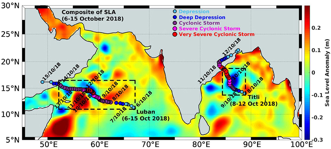
Figure 1. A map showing the North Indian Ocean comprising of the Arabian Sea (AS) and the Bay of Bengal (BoB) with tracks of the cyclones Luban and Titli denoted by the filled circles with different color markers to show the different stages of the cyclone (a cyan circle for depression, a blue circle for deep depression, a purple circle for cyclonic storm, a magenta circle for severe cyclonic storm, and a red circle for very severe cyclonic storm). Shading is the sea level anomaly (SLA) (m). The boxes with broken black lines are the regions that were used for the computation of various parameters. See text for details.

Results and Discussions

Genesis and Evolution of Cyclones Luban and Titli

The simultaneous occurrence of the cyclones Luban (October 6–15, 2018) in the AS and Titli (October 8–12, 2018) in the BoB being an unusual phenomenon, it is important to track their origin and evolution. The daily-mean values of the translation speed, estimated central pressure, and maximum sustained wind speed for Luban and Titli are given in Tables 1, 2, respectively, along with the category of disturbance. Luban was a category-1 (wind speed between 119 and 153 km/h) cyclone, whereas Titli was a category-2 (wind speed between 154 and 177 km/h) cyclone as per the Saffir–Simpson Scale (https://www.nhc.noaa.gov/pdf/sshws_2012rev.pdf). The maximum sustained wind speed of Luban was 75 knots (38.58 m/s; 138.9 km/h), and that for Titli was 80 knots (41.15 m/s; 148.16 km/h), which occurred at 06:00 UTC and 12:00 UTC, respectively on October 10. However, cyclone Titli had an estimated surface wind speed of 140–150 km/h, gusting to 165 km/h during the period 23:00 UTC of October 10 and 00:00 UTC of October 11 when it crossed the coast near Palasa (18.8°N; 84.4°E) of Andhra Pradesh, making it a category-2 cyclone. According to the IMD classification, both were very severe cyclonic storms (VSCS) (as shown in Tables 1, 2). Luban formed as a depression on October 6 over the east-central AS (11.2°N, 67°E, Figure 1) and gradually moved west-northwestwards. It intensified into a deep depression on October 7 at 09:00 UTC, became a cyclonic storm (CS) on October 8 at 03:00 UTC, and then into a severe cyclonic storm (SCS) on October 9 at 09:00 UTC (Figure 1). While moving northwestward on October 10 at 00:00 UTC, it further intensified into a VSCS. The translation speed of the system initially showed a rapid increase from 1.34 m/s on October 6 to 3.87 m/s on October 7, which was 2.9-times higher than the initial value (Table 1). However, the translation speed showed a steady decrease as the system was intensifying and became 1.36 m/s on October 10 when it strengthened into a VSCS. At this time, the system attained a maximum wind speed of 75 kt (38.6 m/s; 138.90 km/h) and the lowest pressure of 978 hPa at 06:00 UTC of October 10 and then continued its west-northwestward movement as a VSCS until 00:00 UTC of October 12. Note that the daily mean of the maximum sustained wind speed on October 10 was lower (72.5 kt, 134.27 km/h, Table 1) than the highest value recorded at 06:00 UTC. At 03:00 UTC of October 10, the system weakened to an SCS, and a CS at 18:00 UTC while moving further northwestward. On October 13, the system continued moving northwestward as a CS and then crossed Yemen and the adjoining Oman coast near 15.8°N and 52.2°E during 05:30 to 06:00 UTC on October 14. On October 15 at 03:00 UTC, the system weakened into a well-marked low pressure area over Yemen and adjoining Saudi Arabia. Interestingly, as the system started dissipating from October 12 to 15, the translation speed showed a rapid increase once again, attaining the highest value of 8.37 m/s (Table 1).

TABLE 1

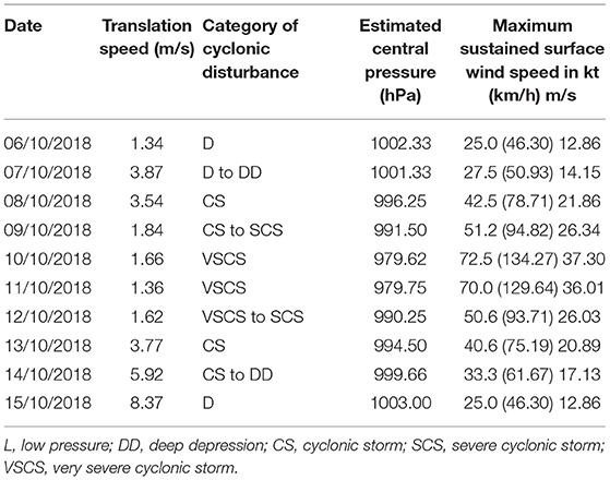
Table 1. Daily mean characteristics of the cyclone Luban in the Arabian Sea (AS) during its genesis and evolution.

TABLE 2

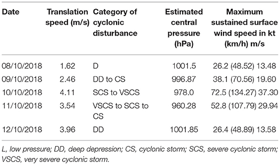
Table 2. Daily mean characteristics of the cyclone Titli in the Bay of Bengal (BoB) during its genesis and evolution.

Cyclone Titli, on the other hand, was formed as a depression in the central BoB (14°N and 88.8°E) on October 8, at 03:00 UTC, and moved in a northwestward direction (Figure 1). On October 9, it became a CS at 06:00 UTC and further intensified into a VSCS on October 10 at 06:00 UTC while moving in a north-northwestward direction. The system was further intensified with a maximum sustained wind speed of 80 kt and the lowest pressure of 972 hPa at 12:00 UTC, while the daily mean of the maximum sustained wind speed was 72.5 kt (Table 2). Contrary to the translation speed of Luban, that of Titli showed a steady increase from October 8 to 10 when the system was intensifying into a VSCS (Table 2). The increase was 2.5 times the initial value of 1.62 m/s. On the same day, during 23:00 UTC, the cyclone crossed the north Andhra Pradesh and south Odisha coast near 18.8°N and 84°E with an estimated surface wind speed of 140–150 km/h, gusting to 165 km/h (Figure 1). As the system gradually reduced its intensity from a VSCS to an SCS on October 11, its translation speed also decreased (Table 2) unlike that of Luban. On October 12, the system weakened into a well-marked low pressure area over Gangetic West Bengal and adjoining Bangladesh.

SST Response

The time evolution of SST before the cyclones Luban (Figure 2A) and Titli (Figure 2D) showed that the eastern and central parts of the AS were at least 2°C warmer than the western part (Figure 2A). In contrast, the SST in most of the BoB was almost the same with values above 29°C (Figure 2D). The colder SST in the western part of the AS was due to the prevailing coastal upwelling during the summer monsoon (Smith and Bottero, 1977; Smith and Codispoti, 1980). Before the formation of cyclone Luban, the SST was 29°C at the location where the cyclone originated and 28°C where the cyclone gained its maximum intensity (Figure 2A). During the period of cyclone Luban, a reduction in SST was noticed along the track (Figure 2B), and after the passage of the cyclone, a cooling of 1.5–2°C was observed at the right side of the track (Figure 2C). Before the formation of cyclone Titli, the SST was 30°C at the location of its origin and 31°C where the cyclone attained its maximum intensity (Figure 2D). During (Figure 2E) and after (Figure 2F) the passage of cyclone Titli, a cooling of 1 and 3°C, respectively, was observed at the right side of the track where the cyclone attained its maximum intensity (Figure 2F).

FIGURE 2

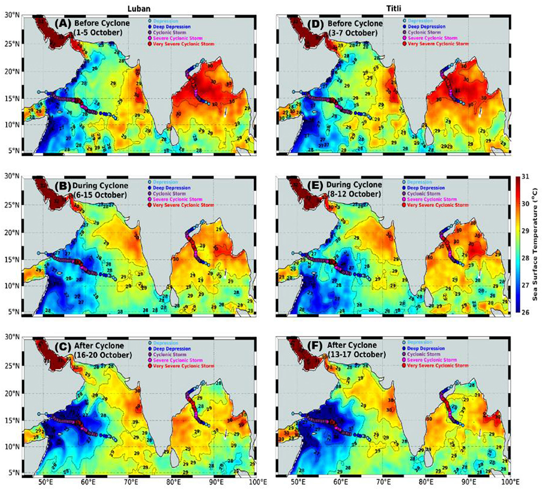
Figure 2. Spatial distribution of the sea surface temperature (SST, °C) before (A,D), during (B,E), and after (C,F) cyclones Luban (A–C) and Titli (D–F), superposed with cyclone tracks.

TCHP Response

The TCHP is a measure of the integrated vertical temperature of the ocean from the surface to the depth of the 26°C isotherm (D₂₆). Being a measure of the heat energy of the ocean, it plays a significant role in the formation and intensification of tropical cyclones. The characteristic feature of the spatial distribution of TCHP was that, although it was higher in the central and eastern regions of both basins, the values prior to the cyclones in the BoB were 20 kJ/cm² higher compared with the AS (Figures 3A,D). In the AS, there was a strong zonal gradient with the lowest values occurring in the western region and close to the southeastern region (Figure 3A). These lowest values were associated with coastal upwelling that occurs along the western boundary and southeastern boundary of the AS, which was also discernible in the spatial distribution of SST in Figure 2A. The cyclone Luban originated from a region in the central AS where TCHP was close to 60 kJ/cm² (Figure 3A). During the cyclone period (Figure 3B), the TCHP values showed a reduction of 20 kJ/cm² toward the west along the track, which was associated with the intensification of Luban into a VSCS on October 10. When Luban moved further westward, it was passing through the region of the lowest TCHP, and that resulted in the weakening of the cyclone. After the passage of Luban, the reduction in the values of TCHP along the track persisted, and the magnitude of reduction was more toward the right side of the track (Figure 3C), consistent with the maximum cooling noticed in the SST (Figure 2C). As the TCHP in the BoB was higher than the AS, the formation of cyclone Titli took place in a region where the TCHP was close to 80 kJ/cm² prior to its formation (Figure 3D). During the active phase of Titli, the TCHP along the cyclone track showed a decrease of nearly 20 kJ/cm² (Figure 3E), a reduction similar to that of Luban. However, unlike Luban, the northwestward track of Titli was through the region of high TCHP. This may be the reason why cyclone Titli was much more intense (Table 2) compared with Luban (Table 1). Similar to Luban, the TCHP values along the track of Titli were also low, with a maximum reduction to the right of the track (Figure 3F).

FIGURE 3

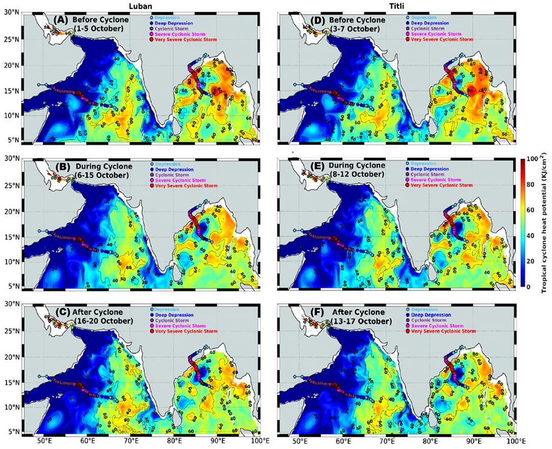
Figure 3. Spatial distribution of the tropical cyclone heat potential (TCHP, kJ/cm²) before (A,D), during (B,E), and after (C,F) cyclones Luban (A–C) and Titli (D–F), superposed with cyclone tracks.

SLA Response

The spatial pattern of SLA overlaid with the geostrophic current before, during, and after the passage of cyclones Luban and Titli (Figure 4) has been analyzed to understand the differences in the life cycle of both cyclones. The blue-colored region with negative SLA indicates the cold-core eddy, and the red-colored region with positive SLA indicates the warm core eddy region (Prasanna Kumar et al., 2004). Prominent circulation features seen prior to the formation of cyclones were the Great Whirl located between 5 and 10°N off the Somali coast and Socotra Gyre (Fischer et al., 1996) and north of the Great Whirl in the AS, with both cold and warm-core eddies located close to the western boundary (Figures 4A,D). In the BoB, three cold-core eddies were present near the western boundary and two warm-core eddies in the offshore region. The origin of cyclone Luban was in a region of positive SLA, and it intensified into a VSCS, while the track was over the edge of Socotra Gyre, a warm core region, and a cold-core eddy (Figure 4B). Its further westward track was over a prominent cold-core eddy region, which may be the reason why the system weakened to an SCS and then to a CS, finally crossing over to Yemen. Notice the change in the circulation pattern by way of the intensification of the cold-core eddy region with a much lower SLA and the reduction in the size of the Socotra Gyre after the passage of Luban (Figure 4C). Unlike Luban, the origin of cyclone Titli was in the region of a warm core eddy (Figure 4D). As it moved northwestward, its track entered into a cold-core eddy region where it intensified from an SCS into a VSCS (Figure 4E). This is an anomaly, as the cyclone is expected to weaken while it is over a cold-core eddy region (Chowdhury et al., 2020b) as it encompasses colder waters compared with its surrounding region. An examination of the SST (Figure 2E) did not show colder waters in the eddy region; instead, the SST was 30°C. This is because, in the BoB, cold-core eddies are usually subsurface, lying just below the warm and thin surface-mixed layer (Prasanna Kumar et al., 2007). Hence, this warm surface water would have helped in the intensification of Titli from an SCS to a VSCS. During its further northward movement, it crossed over a warm core eddy region; after which, the estimated surface wind speed increased to 140–150 km/h, with gusting to 165 km/h. Again, unlike Luban, cyclone Titli crossed the coast as a VSCS and subsequently weakened. The circulation pattern of the western BoB was impacted by the passage of Titli, which resulted in the intensification and expansion of the cold core eddy region over which it passed through (Figure 4F).

FIGURE 4

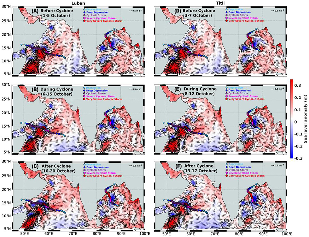
Figure 4. A spatial map of sea level anomaly (m) overlaid with the geostrophic current (m/s) before (A,D), during (B,E), and after (C,F) cyclones Luban (A–C) and Titli (D–F), superposed with cyclone tracks.

Response of Mixed Layer Heat Budget

The dominant response of the upper ocean to both cyclones was the cooling of the sea surface. To understand the roles of different oceanic processes in regulating cyclone-induced upper ocean cooling, the mixed layer heat budget over the box regions (as shown in Figure 1) was computed based on methods described in Section Computation of mixed layer heat budget. The temporal evolution of various terms of the mixed layer heat budget, such as temperature tendency, horizontal advection, net heat flux, and vertical entrainment computed in units of °C/day before, during, and after the passage of cyclone Luban and Titli, was presented in Figure 5. Note that the residual term denotes any processes other than those listed above. The residual term represents unresolved processes, such as turbulent mixing and diffusion. The maximum cooling for Luban was −0.57°C/day (Figure 5A), while that for Titli was −0.44°C/day (Figure 5B), which occurred on October 9 for both cyclones but persisted until October 10 in the case of Titli. The cooling was the combined contributions from the horizontal advection, vertical entrainment, and net heat flux at the sea surface where the cyclones intensified from a CS to an SCS/VSCS. Note that the contribution of vertical entrainment was very small for both Luban and Titli during the study period. During the peak cooling, the horizontal advection contributed 0.10 and −1.77°C/day, respectively, for Luban and Titli. In the case of Luban, the net heat flux showed a rapid decrease from the pre-cyclone value of 0.2°C/day to almost zero when the temperature tendency showed the lowest value (highest cooling). This indicated that the rapid decline in the temperature tendency was contributed by horizontal advection and residual. However, after the passage of cyclone Luban, the net heat flux showed a rapid increase in its pre-cyclone value, while the temperature tendency more or less maintained its pre-cyclone value. This indicated that the temperature tendency was controlled by the balance between the increasing net heat flux and the declining horizontal advection along with the residual.

FIGURE 5

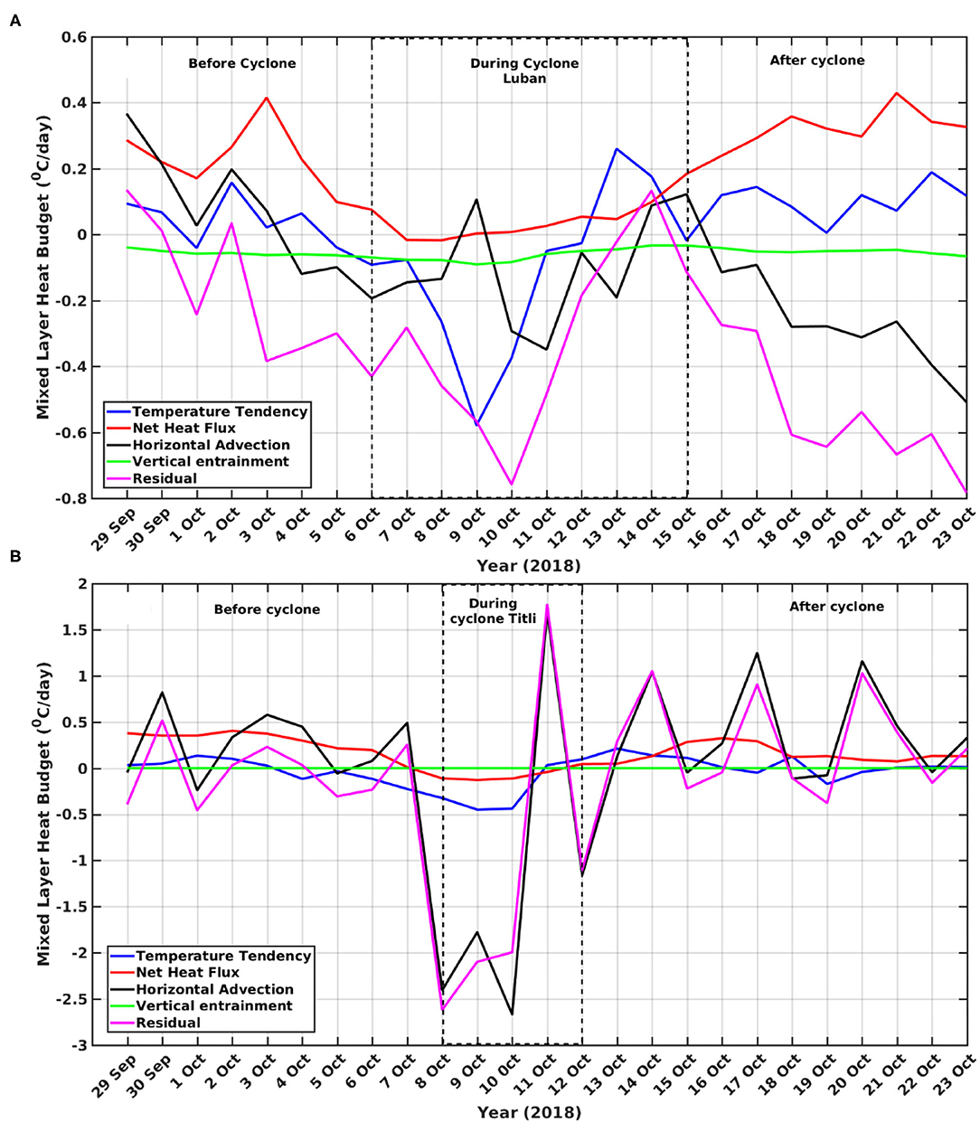
Figure 5. Variation of mixed layer heat budget terms (°C/day) before, during, and after the passage of the Luban (A) and Titli (B) cyclones. The box with a black broken line over the curve indicates the period of the cyclone.

The time evolution of the response of the mixed layer heat budget under the influence of cyclone Titli (Figure 5B) was somewhat different in comparison to Luban. Although the magnitude of the variation of temperature tendency and net heat flux associated with Titli were similar to that of Luban, the horizontal advection and residual showed a much higher magnitude of variation. In fact, during the period of cyclone Titli, horizontal advection and residual showed the highest negative value (~-2.5°C/day) on October 8/9, when the cyclone was intensifying, while the highest positive value (~1.5°C/day) was on October 11, when the cyclone was weakening (Figure 5B). However, in spite of these large variations in the horizontal advection and residual, the temperature tendency (peak cooling) during Titli was comparable to that of Luban. This implies a large modification to the surface currents under Titli compared with Luban, which is corroborated by a comparison of the geostrophic flow fields before and after the passage of cyclones (Figures 4D,F). Note that the pattern of variability of the horizontal advection and residual before and after the passage of cyclone Titli was similar and worked in tandem with net heat flux to maintain the temperature tendency. It is important to state the limitation in the present study in deciphering the possible causes for the high values of the residual term. In the mixed layer heat budget equation (Equation 8), the residual term is the estimation of error that comes along with the horizontal and vertical eddy diffusion. As all the terms of the equation are calculated based on different sets of data, having different horizontal and vertical resolutions, there is a possibility of error accumulation during the interpolation of such heterogeneous data as indicated in Liang et al. (2019), in addition to unresolved ocean dynamic processes. Although we do not have any information on the unresolved processes that contributed to the residual, it is worth mentioning that the cyclone-induced enhanced evaporative cooling and upward Ekman pumping of cold subsurface waters would influence the mixed layer temperature tendencies under a cyclone. After the passage of cyclones, temperature tendencies were dominated by net heat flux, horizontal advection, and the residual terms of the mixed layer.

Response of Water Mass Characteristics

The characteristics of the water masses present in the upper 200 m of the water columns in the AS and the BoB are different. To understand the upper ocean water mass variability due to the passage of cyclones Luban and Titli, potential temperature vs. salinity was plotted (θ-S diagram) at the location where both the cyclones attain their maximum intensity, following Chowdhury et al. (2020b). The location of the cyclones on October 10 at 12:00 UTC (14.7°N; 51.7°E for Luban and 17.5°N; 85.3°E for Titli; as shown in Figure 1) was taken as a center, and a 0.5°latitude × 0.5°longitude box around it was considered for computing the box-averaged potential temperature (θ) and salinity. The HYCOM temperature and salinity profiles up to the 200-m depth of October 5 and 16 were used as before and after the cyclone, respectively, for computing the θ-S diagram for Luban (Figure 6A). Similarly, the temperature and salinity profiles of October 7 and 13 were used as before and after the cyclone, respectively, for computing the θ-S diagram for Titli (Figure 6B). Two water masses were identified from the θ-S diagram in the AS, such as the Arabian Sea High Salinity Watermass (ASHSW) and the Persian Gulf Water mass (PGW), having sigma-θ values of 22.8–24 and 26.2–26.8 kg/m³, respectively. Before the formation of cyclone Luban, the θ-S diagram on October 5 (blue line in Figure 6A) showed the presence of ASHSW in the upper 20 m with salinity maxima at 10 m, while the PGW was located between 150 and 250 m with a high-salinity core at 200 m (Figure 6C). After the passage of cyclone Luban (green line in Figure 6A), the ASHSW deepened to a ~25-m depth, while the PGW deepened to a below 350-m depth (Figure 6C). Apart from deepening due to intense mixing, both water masses were subjected to cooling and freshening as could be inferred from the vertical profiles of the temperature and salinity in the upper 400 m (Figure 6C). In the case of ASHSW, it was cooled by 2.7°C, and salinity was lowered by 0.22 units. In the case of PGW, it was cooled by 1.8°C, and salinity was lowered by 0.12 units.

FIGURE 6

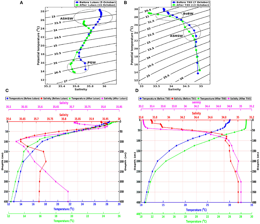
Figure 6. θ-S diagram (0–200 m depth) for Luban (October 5 and 16) (A), Titli (October 7 and 13) (B) before (blue line), and after (green line) cyclones. A black solid line indicates the sigma-θ line. ASHSW, Arabian Sea High Salinity Water mass; PGW, Persian Gulf Water mass. The vertical profiles of temperature and salinity (0–400 m) before and after Luban (C) and Titli (D). Blue and green lines show the temperature profile, while red and magenta lines show the salinity profiles before and after the cyclones, respectively.

In the BoB, two water masses were also identified such as the Bay of Bengal water mass (BoBW) and the ASHSW (Figure 6B). Before the cyclone, the Titli, θ-S diagram (blue line) showed the presence of BoBW and ASHSW, having sigma- θ values of 21–23 and 22.8–24 kg/m³, respectively. Prior to the formation of cyclone Titli, the θ-S curve on October 7 (blue line in Figure 6B) showed the presence of low-salinity BoBW in the depth range of 20–30 m, while the ASHSW was located in the depth range of 70–80 m (Figure 6D). After the passage of cyclone Titli, the BoBW deepened and occupied the depth range of 20–40 m, and the ASHSW was deepened to a 100-m depth. The entrainment and mixing in the case of Titli (Figure 6B) were much less intense compared with Luban (Figure 6A) as could be inferred from the shift of the θ-S curves before (blue) and after (green) the cyclones. Under the entrainment and mixing, the BoBW cooled by 1.09°C, and the salinity was decreased by 0.51 units (Figure 6D).

Cyclone-Induced Biological Response

Having examined the physical and dynamic responses of the upper ocean due to the passage of cyclones Luban and Titli, we now analyze the biogeochemical response in this section. To understand the biological response, the 3-day composites of the Chl-a and NPP before, during, and after cyclone were analyzed within the boxes (as shown in Figure 1). While plotting the 3-day composite figures, the average values of Chl-a and NPP were assigned to the day between the beginning and the end when the 3-day composite was calculated. For example, the 3-day averaged values computed for Chl-a and NPP during the period from September 29 to October 1 were assigned to September 30 in the plot.

The average Chl-a before the origin of cyclone Luban was 0.61 ± 0.11 mg/m³, and it increased to a maximum value of 1.22 ± 0.11 mg/m³, which occurred in the 3-day composite period between October 17 and 19 after the passage of the cyclone (Figure 7A). Note that the initial decline in Chl-a concentration during the cyclone must be due to the thick cloud cover that cuts off the visible radiation from the ocean. A similar situation was reported by Byju and Prasanna Kumar (2011) in the case of cyclone Phyan in the AS, and they showed that the initial decline in Chl-a was due to a decrease in the number of data pixels in the study region due to cloud cover associated with the cyclone. Once the cyclone moves out of the study region, the sky clears off, and the pixel count increases and captures well the variability in Chl-a. Note also that the peak Chl-a, which was 2-fold higher than the pre-cyclone value, occurred 3 days after the dissipation of the cyclone. Within a week after the passage of cyclone, the enhancement of Chl-a declines and attains its pre-cyclone values. The Chl-a response of the BoB to cyclone Titli (Figure 7B) was similar to that of the AS to cyclone Luban, except for the magnitude. The average Chl-a before cyclone Titli was 0.29 ± 0.05 mg/m³, which showed a 3-fold increase after the passage of a cyclone. Similarly, during the initial phase of Titli, the Chl-a showed a decline, and it peaked at 0.88 ± 0.07 mg/m³ after 5 days of its dissipation.

FIGURE 7

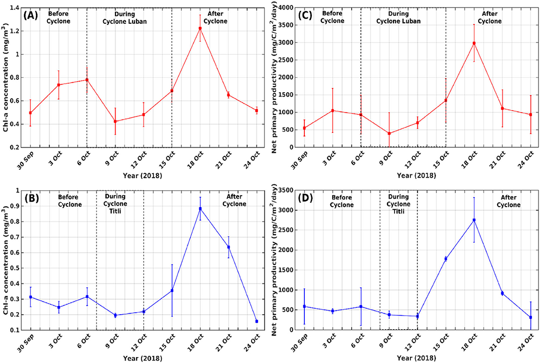
Figure 7. Box-averaged 3-day mean chlorophyll a (Chl-a) concentration (mg/m³) and net primary productivity (mg/C/m²/day) before, during, and after the passage of cyclone Luban (A,C) and cyclone Titli (B,D) from September 29 to October 25, 2018. The box with a black broken line over the curve indicates the period of the cyclone.

The time variation of NPP under the influence of both cyclones (Figures 7C,D) showed a pattern that was very similar to that of the Chl-a variation. Before the passage of cyclone Luban, the average value of NPP was 799.77 ± 431.58 mg C/m²/day (Figure 7C). Consistent with the Chl-a, the value of NPP showed a small decline during the initial period of the cyclone and then increased to a maximum value of 2,980.90 mg C/m²/day after the passage of the cyclone. The NPP enhancement after the cyclone Luban was 3.7-times its pre-cyclone value. Unlike Luban, the NPP did not show much variation before the cyclone Titli (Figure 7D). The average NPP value before Luban was 544.94 ± 327.93 mg C m²/day, and it showed a small decline during the period of the cyclone. The maximum value of 2,752.00 ± 560.66 mg C m²/day occurred in the 3-day composite period between October 17 and 19 after the passage of the cyclone. The NPP enhancement after the cyclone Titli was five times its pre-cyclone value. A pertinent question would be why there is a lag between the passage of a cyclone and the peaking of Chl-a and NPP. This is the biological response time for the photosynthesis to start (NPP) and, eventually, to build up the chlorophyll biomass (Chl-a). This can be understood in the following manner. The anti-clockwise winds associated with the cyclone will create a divergence of the surface water and initiate upward Ekman pumping (Subrahmanyam et al., 2002; Lin et al., 2003). This will bring subsurface nutrient-rich colder waters to the surface. Although there is a build-up of surface nutrient concentration, the phytoplankton present in the water column is unable to carry out photosynthesis due to the light limitation because of cloud cover. Once the cyclone moves away from the region, the sky is cleared of clouds, allowing the sunlight to reach the upper ocean, which will kick-start the biological production through photosynthesis. Hence, there is always a lag between the cyclone-induced nutrient supply to the oligotrophic upper ocean and its response by way of the enhancement of Chl-a and NPP (Byju and Prasanna Kumar, 2011; Chowdhury et al., 2020a,b).

Thus, there was a striking similarity between the time evolution of Chl-a and NPP in response to cyclones in both the AS and the BoB. Although the pattern of variability was similar, the magnitudes of both were higher in the AS than in the BoB. The pre-cyclone Chl-a concentration in the AS was three times higher than that in the BoB, while NPP was 1.5 times higher than that in the BoB. However, the maximum NPP did not show much difference between the AS and the BoB, although the maximum enhancement of Chl-a in the AS was 1.4 times higher than that in the BoB. The AS is also known for its high values of Chl-a and NPP compared with the BoB, which is linked to the differences in the regional oceanographic processes between the AS and the BoB (Prasanna Kumar et al., 2009b). With October being the period of secondary heating, the thermal stratification is high in both the AS and the BoB (Prasanna Kumar and Narvekar, 2005; Narvekar and Prasanna Kumar, 2006). In addition, in the BoB, the freshwater flux due to the precipitation and river runoff peaks in October leads to the strongest haline stratification (Narvekar and Prasanna Kumar, 2014). Strong upper ocean stratification in the BoB in comparison to the AS curtails the vertical mixing due to wind, thereby limiting the availability of nutrients in the upper ocean. This is the reason for the lower pre-cyclone Chl-a and NPP in the BoB compared with the AS. However, being a category-2 cyclone, Titli could potentially initiate stronger vertical transport of cold and nutrient-rich waters to the upper ocean compared with the category-1 Luban. The 5-fold increase of NPP by Titli in comparison to the 3.7-fold increase by Luban lends support to this.

Response of CO₂ Flux

The air-sea CO₂ flux at the sea surface has an impact on the storage of anthropogenic CO₂ in the ocean (Takahashi et al., 2009). Air-sea CO₂ flux depends on the difference between the partial pressure of CO₂ at the surface and in the atmosphere, wind speed, SST, and sea surface salinity (Wanninkhof, 1992). Wind speed plays the most important role in the variability of CO₂ flux due to the quadratic functional dependence of gas transfer velocity and wind speed. Studies have suggested that strong winds associated with tropical cyclones increase the CO₂ flux from the ocean to the atmosphere (Bates et al., 1998; Bates and Peters, 2007; Nemoto et al., 2009). To understand the changes in the CO₂ flux from the ocean to the atmosphere under the influence of Luban and Titli, we have analyzed the cyclone-induced CO₂ flux in the box region (see Figure 1). Before cyclone Luban, the average CO₂ flux value was 0.65 ± 0.11 mmol/m²/day (Figure 8A). During the cyclone, the values showed a rapid increase, and the maximum value of 6.41 ± 1.01 mmol/m²/day was on October 9, which was almost approximately a 10-fold increase compared with the pre-cyclone value. Note that the intensification of Luban to an SCS occurred on October 9, when the box-averaged CO₂ flux showed a maximum value. However, the CO₂ flux value on October 10 was only marginally low, which was when Luban further intensified to become a VSCS. The upward Ekman pumping velocity (EKV) (not shown) was maximum on October 9, and the value was 0.55 m/day. During a cyclone, an upward EKV brings subsurface waters with high CO₂ to the surface and causes CO₂ efflux or/outgassing. Positive values of CO₂ flux indicate the release of CO₂ from the ocean to the atmosphere. The value of CO₂ flux on October 10 during cyclone Luban was 6.22 ± 0.67 mmol/m²/day (Figure 8A). As the cyclone started reducing its intensity after October 10, the CO₂ flux values also showed a rapid decline and attained the pre-cyclone values after the passage of the cyclone. In the case of Titli, the CO₂ flux before the cyclone was 0.76 ± 0.08 mmol/m²/day (Figure 8B). During the cyclone, the maximum CO₂ flux was observed on October 10, and the value was 9.23 ± 0.91 mmol/m²/day. Recall that Titli attained its maximum intensity as a VSCS on October 10. The upward EKV (not shown) was maximum on the October 10, and the value was 0.8 m/day. Like cyclone Luban, the CO₂ flux values showed a rapid decline after the passage of Titli from the box region. The maximum CO₂ flux associated with Titli was a 12-fold increase compared with its pre-cyclone value.

FIGURE 8

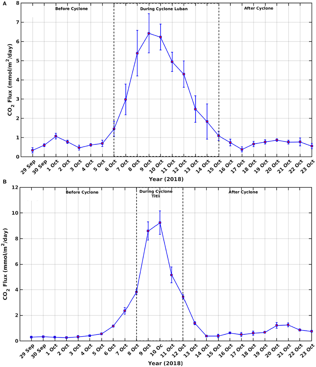
Figure 8. Box-averaged daily CO₂ flux (mmol/m²/day) over the box region before, during, and after the passage of cyclones Luban (A) and Titli (B) from September 29 to October 23, 2018. The box with a black broken line over the curve indicates the period of the cyclone.

Atmospheric Conditions Before, During, and After Cyclone

Having deciphered the physical and biogeochemical response of the upper ocean to the passage of cyclones Luban and Titli, in this section, the atmospheric variables related to cyclone genesis and intensification, namely, low-level wind convergence, low-level relative vorticity, vertical wind shear, and mid-tropospheric relative humidity, were examined. It is well-known that, for the generation of a tropical cyclone, the necessary conditions of the above variables are strong low-level wind convergence, high-relative vorticity, weak vertical wind shear, and high-relative humidity (Evan and Camargo, 2011). Strong low-level wind convergence is associated with strong convection, and OLR is a proxy for convection. Hence, the spatial maps of OLR (Figure 9), the relative vorticity at 850 hPa (Supplementary Figure 1), the vertical wind shear between 850 and 200 hPa (Figure 10), and the relative humidity at 500 hPa (Figure 11) were prepared and presented below.

FIGURE 9

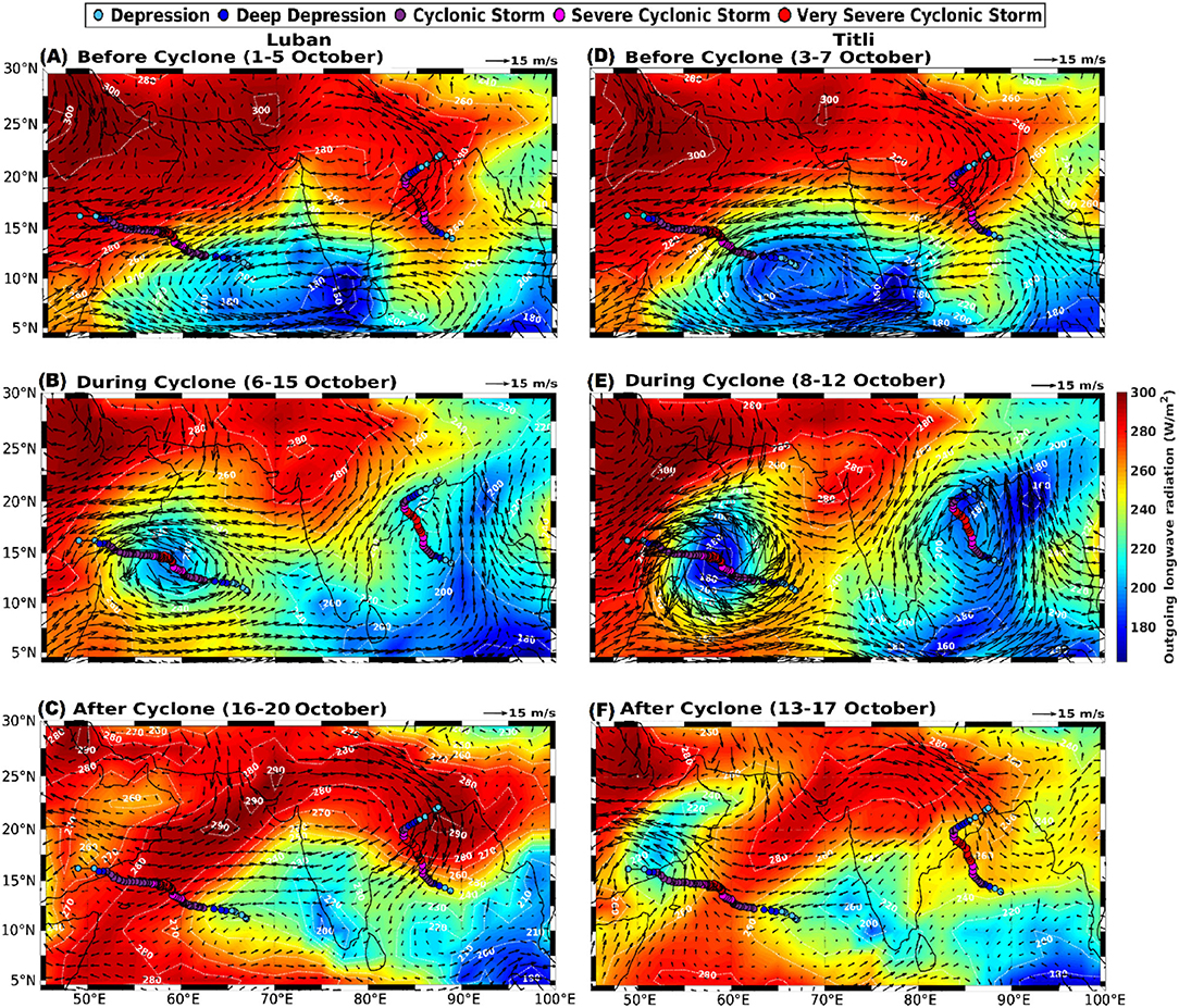
Figure 9. A spatial map of outgoing longwave radiation (W/m²), overlaid with 850 hPa wind (m/s) before (A,D), during (B,E), and after (C,F) cyclones Luban (A–C) and Titli (D–F). The color-filled circles denote the cyclone tracks.

FIGURE 10

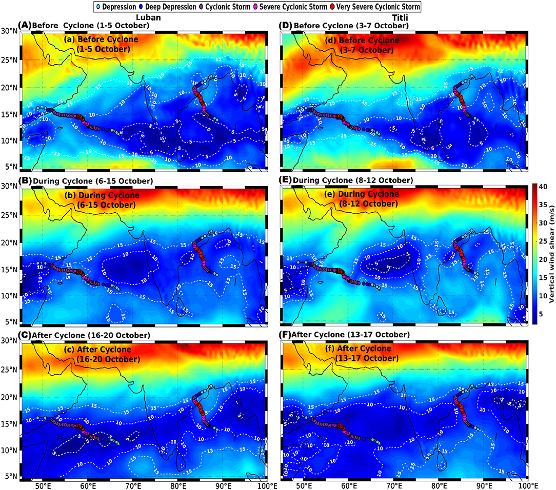
Figure 10. A spatial map of vertical wind shear (difference between 200 and 850 hPa) (m/s) before (A,D), during (B,E), and after (C,F) cyclones Luban (A–C) and Titli (D–F). The color-filled circles denote the track of the cyclone.

FIGURE 11

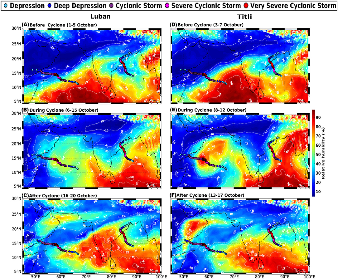
Figure 11. A spatial map of mid-tropospheric (500 hPa) relative humidity (%) before (A,D), during (B,E), and after (C,F) cyclones Luban (A–C) and Titli (D–F). The color-filled circles denote the cyclone.

The OLR, in general, showed low values in the southern part of the study region and increased toward the north (Figure 9). Prior to the formation of both cyclones, the OLR values were low and close to 200 and 220 W/m² in the region of origin of Luban (Figure 9A) and Titli (Figure 9D), respectively. The large-scale easterly and northeasterly winds showed convergence in the region of origin of Luban and Titli (Figures 9A,D). The low OLR along with wind convergence indicated strong convection, a condition that is favorable for the formation of cyclones. The spatial distribution of relative vorticity showed high positive values in the region of origin of Luban (Supplementary Figure 1A) and Titli (Supplementary Figure 1D), while the vertical wind shear was the least, 5 m/s, at the origins of Luban (Figure 10A) and Titli (Figure 10D) prior to the formation of both the cyclones. The mid-tropospheric relative humidity, on the other hand, was high with values of 80 and 70%, respectively, in the region of Luban (Figure 11A) and Titli (Figure 11D). Thus, the atmospheric condition by way of the low OLR, high-positive-relative vorticity, low-vertical wind shear, and high-relative humidity set the stage for the formation of cyclones Luban and Titli.

During both the cyclones, the OLR along the track and in its vicinity was low with strong cyclonic circulation (Figures 9B,E), while the wind shear increased to ~15 m/s (Figures 10B,E). The vorticity showed a general increase along the track for both Luban (Supplementary Figure 1B) and Titli (Supplementary Figure 1E). The relative humidity, however, decreased to 40–50% in the case of Luban (Figure 11B) and 50–70% for Titli (Figure 11D). After the passage of the cyclones, the values of all the atmospheric parameters showed a recovery toward the pre-cyclone values.

Potential Mechanism for the Simultaneous Generation of Cyclones

The formation of tropical cyclones requires a large amount of thermal energy to be available in the upper ocean in the form of TCHP. However, the mere availability of TCHP alone will not lead to the formation of a cyclone. Cyclogenesis would need the pre-conditioning of several ocean-atmospheric parameters, as indicated in the previous section, followed by a triggering mechanism. To gain insight into the ocean-atmospheric dynamics that lead to the simultaneous formation of cyclones Luban in the AS and Titli in the BoB, we examined the interannual and intraseasonal variability that could potentially suggest such mechanism/s.

Role of Climate Modes

Climate modes, such as the Pacific decadal oscillation (PDO), El Niño Southern Oscillation (ENSO), and IOD, influence the tropical Indian ocean on an interannual time scale. Recently, Girishkumar and Ravichandran (2012) and Sreenivas et al. (2012) studied the role of ENSO in the formation of tropical cyclones in the BoB during the October–December period. To understand how the above modes influence the AS and the BoB, the indices associated with these modes was analyzed from 1979 to 2020 and presented in Supplementary Figure 2. The indices are the Pacific decadal oscillation index for PDO (Supplementary Figure 2A), Nino-3.4 index for ENSO (Supplementary Figure 2B), and dipole mode index for IOD (Supplementary Figure 2C). The year 2018 showed the presence of moderate El Niño and positive IOD, while the PDO was in the cold phase. The co-occurrence of El Niño and positive IOD in 2018 (Supplementary Figures 2B,C) made the waters of the eastern Indian Ocean colder than normal, along with the prevalence of the descending branch of Walker circulation (Walker and Bliss, 1932), while the waters of the western Indian Ocean become warmer than normal, along with the prevalence of the ascending branch of Walker circulation (as shown in Chowdhury et al., 2020a). This would make the AS and part of the BoB warmer than normal. The negative values of the PDO index (Supplementary Figure 2A), which indicated that 2018 was in the cold phase, were associated with warm SST anomalies in the north, west, and southern Pacific (Mantua et al., 1997; Mantua and Hare, 2002). Thus, all three climate modes in 2018 were congenial for creating warmer than the normal upper ocean. The SST anomaly for the year 2018 clearly showed a warm anomaly of 0.5°C in the region where cyclones Luban and Titli originated (Supplementary Figure 3), which corroborates the fact that all the three climate modes acted in tandem to make 2018 a warmer than normal year. Although a warm SST is one of the necessary conditions for cyclogenesis, other conditions also need to be met. So, next, we examined the intraseasonal variability to see what was unique in 2018 that would have supported the generation of cyclones simultaneously.

Role of Intraseasonal Variability

We examined two types of intraseasonal variability associated with the atmospheric phenomena, such as the mixed Rossby-gravity wave and the MJO, and the oceanic Rossby wave.

Mixed Rossby-Gravity Wave

Mixed Rossby-gravity waves (Hayashi, 1974; Hayashi and Golder, 1978) are equatorially trapped planetary waves that form an integral part of the tropical atmospheric circulation (Matsuno, 1966). They are generated in the troposphere, having a wavelength of 9,000 km and a period of 4–5 days, and form an integral part of the tropical atmospheric circulation (Matsuno, 1966). These waves originate from the lower troposphere and propagate vertically. The energy propagation of Mixed Rossby-gravity (MRG) waves is in an eastward and downward direction, while their phase propagation is westward and upward. The asymmetric warming pattern on either side of the equator during October, associated with the period of secondary heating (Prasanna Kumar and Narvekar, 2005), triggers an MRG wave-type disturbance. To assess the presence of such a disturbance, the time-longitude Hovmöller diagram using a high-frequency (2–10 days) bandpass filtered meridional wind component at the lower (850 hPa) and upper (200 hPa) troposphere was prepared and is presented in Figure 12. The Hovmöller diagram of the meridional wind at 850 hPa revealed the presence of the westward propagation of high positive values of the meridional wind at the lower troposphere, starting from September 1 in the eastern Indian Ocean and reaching the site of origin of Luban by October 6, the day when the depression was formed (Figure 12A). A similar eastward propagation feature could be noticed in the Hovmöller diagram of the meridional wind at 200 hPa (Figure 12B). This was the signature of the MRG wave. However, no such prominent propagation feature was noticed in the vicinity of the site of origin of Titli.

FIGURE 12

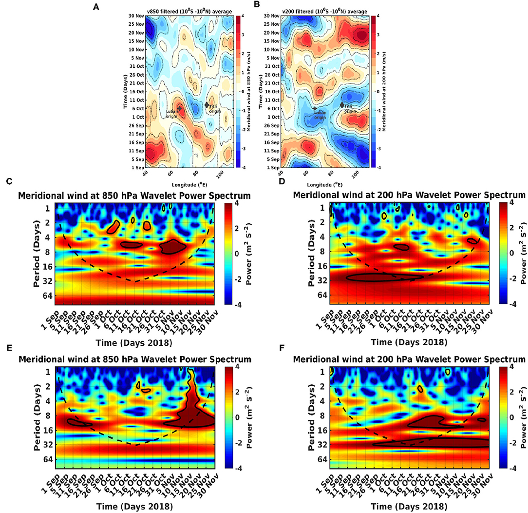
Figure 12. A time-longitude Hovmöller diagram of filtered meridional wind (m/s) at 850 hPa (A) and 200 hPa (B) averaged over 10°S to 10°N from September 1 to November 30, 2018. Black asterisk and diamond symbols show the origin of cyclones Luban and Titli, respectively. Wavelet power spectrum analysis of meridional wind (m² s⁻²) at 850 hPa (C,E) and 200 hPa (D,F) at the origin of cyclones Luban and Titli from September 1 to November 30, 2018. The black broken line represents the cone of influence, and, beyond that line, wavelet power can be distorted (less reliable). The black solid contoured regions show the power, which is 95% significant.

To further ascertain the presence of the MRG wave, we have carried out the continuous wavelet transform analysis using the 6-h meridional wind data of the lower and upper troposphere in the vicinity of Luban (Figures 12C,D) and Titli (Figures 12E,F) by taking a 1-degree-longitude by a 1-degree-latitude box with the origin of the cyclone as the center. The wavelet power spectrum analysis in the region of origin of cyclone Luban confirmed the presence of a 5- to 8-day periodicity in the lower (Figure 12C) and upper (Figure 12D) troposphere. The 5- to 8-day periodicity noticed in the meridional wind at the lower and upper troposphere was significant at the 95% confidence level; however, no such periodicity was noticed in the case of Titli (Figures 12E,F). Thus, the wavelet analysis confirms the presence of MRG waves of 5- to 8-day periodicity in the vicinity of Luban during the period of the cyclone. The MRG waves originate at the lower troposphere and are forced to propagate vertically, and the associated surface convection is responsible for ascending moisture to the middle troposphere. The mid-tropospheric-relative humidity makes the layer convectively unstable, leading to the formation of deep convection, which is conducive for the initiation of MJO and propagation (Muraleedharan et al., 2015). To determine the presence of MJO, we have analyzed the MJO phase space diagram.

Madden–Julian Oscillation

The MJO is a dominant mode of atmospheric variability in the tropical region in the intraseasonal time scale, which has a periodicity of 30–90 days (Madden and Julian, 1971). The MJO propagates eastward in boreal winter and northward in boreal summer (Zhang, 2005). Camargo et al. (2009) showed that MJO plays an important role in the genesis of cyclones in the Indian Ocean. To determine the role of MJO in initiating the cyclone, we have calculated the real-time multivariate MJO principal component time series 1 and 2 (RMM1 and RMM2) using the first two empirical orthogonal functions of equatorially averaged OLR and lower-level (850 hPa, and upper-level (200 hPa) wind data. See Wheeler and Hendon (2004) for computation details.

Prior to the formation of cyclone Luban, MJO was in active Phase 1 (Figure 13A). On October 6, cyclone Luban originates in the AS when MJO was in Phase 1, and it started to move toward the Indian Ocean region. The dissipation of cyclone Luban occurred on October 15, when MJO was in Phase 3 and activity was strong. Similarly, cyclone Titli was formed in the active MJO phase. The genesis and dissipation of cyclone Titli were formed in Phase 2. To understand MJO propagation, we have analyzed the time-longitude section of the 30- to 90-day bandpass-filtered OLR (Figure 13B) and the zonal wind at 850 hPa averaged over 10°S to 10°N (Figure 13C). The blue region in OLR having negative values (Figure 13B) showed the enhanced convection, whereas the positive value in the red region indicated the suppressed convection. The zonal wind with positive values with the red color (Figure 13C) indicated the westerly wind, and the blue color having negative values indicated the easterly wind. The eastward propagation of MJO is seen from the time-longitude plots of zonal wind. The OLR showed the presence of enhanced convection on October 6, while zonal wind showed the presence of an active phase of MJO at the location of Luban. After the formation of Luban, the convection associated with MJO moved eastward. The MJO associated with easterly wind and enhanced convection reached the BoB on October 8. The enhanced convection associated with anomalous easterlies was conducive for the formation of the second cyclone, Titli.

FIGURE 13

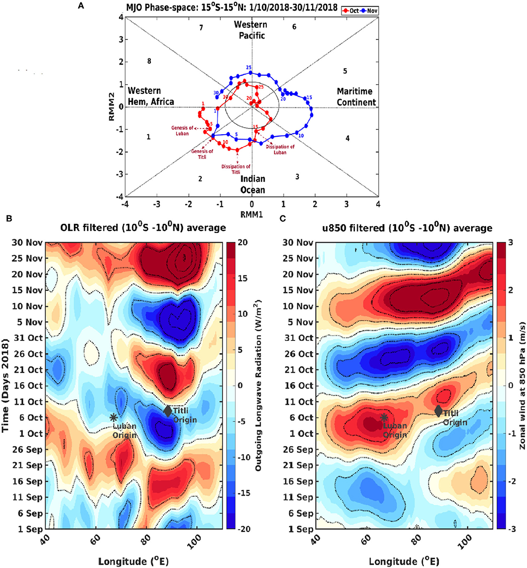
Figure 13. (A) A phase diagram of the Madden-Julian oscillation (MJO) from September 1 to November 30, 2018. The red and blue colors denote the propagation in October and November, respectively. MJO activity is weak (strong) when the index is within (outside) the circle, (B) a time-longitude Hovmöller diagram of 30- to 90-day band-pass-filtered outgoing longwave radiation (W/m²), and (C) zonal wind (m/s) at 850 hPa (C), averaged over 10°S to 10°N from September 1 to November 30, 2018. Black asterisk and diamond symbols show the origin of cyclones Luban and Titli, respectively.

It is, thus, amply clear that, while PDO, ENSO, and IOD pre-conditioned the upper waters in the vicinity of the origin of Luban and Titli by providing excess heat, the atmospheric MRG waves along with MJO provided the trigger for the initiation of Luban. To understand what could be the trigger for Titli, we analyzed the oceanic Rossby waves as a potential remote force.

Oceanic Rossby Wave

The oceanic Rossby wave excited by the coastally trapped Kelvin wave plays an important role in the dynamics and circulation in the BoB (Potemra et al., 1991; Yu et al., 1991). It also modulates the upper ocean through thermocline variations. Recall that the TCHP in the BoB, especially in the region of the formation of Titli, was 20 kJ/cm² higher than that in the AS prior to the formation of the cyclone. We examined the role of the Rossby wave in altering the TCHP in the BoB by analyzing the time-longitude Hovmöller plots of SLA, D₂₆, and TCHP along 14°N by averaging values between the 13.5 and 14.5°N (Figure 14). The Hovmöller plot of SLA (Figure 14A) showed the westward propagation of a high positive SLA in the vicinity of the origin of Titli, which was the signature of a downwelling Rossby wave. The downwelling Rossby wave reached the location of the origin of Titli in the first week of October. Consistent with this, the Hovmöller plot of D₂₆ showed the deepening of the ocean surface layer up to the 80-m SLA (Figure 14B), while the Hovmöller plot of TCHP enhanced to 60 kJ/cm² (Figure 14C). Thus, the downwelling Rossby wave leads to an enhancement of TCHP in the location of the origin of Titli in the first week of October by deepening the thermocline.

FIGURE 14

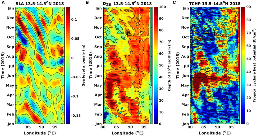
Figure 14. A time-longitude Hovmöller diagram of (A) SLA (m), (B) D₂₆ (m), and (C) TCHP (kJ/cm²) from January 1 to December 31, 2018, averaged over 13.5–14.5°N latitude. A black asterisk denotes the location of the origin of the cyclone Titli.

Summary and Conclusion

The simultaneous occurrence of cyclones over the AS and the BoB in the NIO is an unusual phenomenon that happened in October 2018 for the first time since the reliable record became available in 1960. The physical and biogeochemical responses due to the passage of category-1 cyclone Luban (6–15 October) in the AS and category-2 cyclone Titli (8–12 October) in the BoB have been analyzed using various ocean and atmosphere datasets. The higher TCHP in the BoB compared with the AS was one of the reasons why Titli was more intense than Luban. Another reason was that, while moving westward/northwestward, Luban encountered regions with waters colder by 2°C and TCHP lower by 20 kJ/cm² in comparison to Titli. This is because the western AS was colder due to the upwelling along the western boundary, while no such upwelling occurs in the BoB. In response to the passage of Luban, the surface water showed a maximum cooling of 2°C, while that by Titli was 3°C. The contrast in the cyclone-induced changes was more pronounced in the biogeochemical parameters. The Chl-a and NPP enhancements by Luban were 2 and 3.7-fold, respectively, compared with the pre-cyclone values, while that by Titli were 3 and 5-fold, respectively. Although there were strong similarities between the time evolution of Chl-a and NPP in the AS and the BoB, their values were higher in the AS compared with the BoB. This is because the upper ocean stratification in the BoB was stronger compared with that in the AS. Similar to the biological parameters, the CO₂ flux under Luban showed a 10-fold increase in comparison to the pre-cyclone value, while that under Titli was 12-fold. Based on the data analysis, it was found that the cyclone in the BoB had more influence on the enhancement of phytoplankton biomass and primary production compared with the AS. However, unlike the Chl-a and NPP, the magnitude of CO₂ outgassing in the BoB was higher than that in the AS. This is because of the warmer SST in the BoB and the stronger wind speed associated with Titli, both of which control the magnitude of the CO₂ outgassing.

The most intriguing question is: What triggered the simultaneous occurrence of Luban and Titli? Being an energy-intensive process, the genesis of cyclones requires a large amount of thermal energy close to the upper ocean with a high SST. The year 2018 was an unusual year when both El Niño and IOD co-occurred and PDO was in the cold phase. All three climate modes acting in tandem led to the warming of the upper ocean in the AS and part of the BoB by 0.5°C compared with the climatological mean value. This excess warming pre-conditioned the upper ocean by making higher-than-normal thermal energy available for the formation of cyclones by way of TCHP. It is the arrival of MJO and the MRG wave in the first week of October in the vicinity of the origin of cyclone Luban in the AS that initiated a basin-wide air-sea interaction, which acted as a trigger for the generation of Luban on October 6. In the case of Titli, the triggering mechanism was the arrival of MJO and the oceanic Rossby wave in the vicinity of the origin of Titli on October 8. The eastward propagation of enhanced convection associated with MJO and the shifting of low vertical wind shear and high mid-tropospheric humidity created a favorable condition for cyclogenesis. Along with this, the westward propagating downwelling Rossby wave depressed the thermocline, which increased TCHP and augmented the genesis of cyclones. The above mechanisms explaining the simultaneous occurrence of Luban and Titli in the NIO are schematically shown in Figure 15.

FIGURE 15

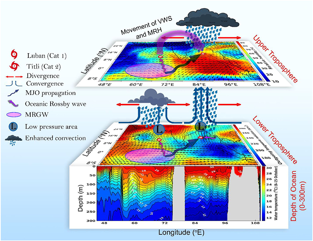
Figure 15. A schematic diagram represents the ocean-atmosphere dynamics associated with the simultaneous genesis of cyclone Luban in the AS and Titli in the BoB over the North Indian Ocean. The lower (vertical) panel depicts the vertical temperature structure during October 6–15, 2018 (the cyclone period) in the upper 300-m depth. The middle (horizontal) panel depicts the outgoing longwave radiation (W/m², shading), superposed with the lower tropospheric wind (m/s) at 850 hPa, and the upper (horizontal) panel depicts mid-tropospheric-relative humidity (%, shading) at 500 hPa, superposed with the upper tropospheric wind (m/s) at 200 hPa. VWS and MRH denote vertical wind shear and mid-tropospheric-relative humidity, respectively, moving from the AS to the BoB, indicated by the curved thick magenta arrow. MJO and MRGW stand for Madden–Julian oscillation and mixed Rossby-gravity wave. Refer to text for details.

The complex dynamics of tropical cyclones involve mixed layer dynamics, planetary waves, intraseasonal variability, and climate modes. An intuitive mechanistic understanding of such interactions, although possible through extensive data analysis as done in the present study, still needs high-resolution coupled-model studies and near real-time observations for a quantitative understanding and better prediction of cyclones. As climate models continue to project the rapid warming of the NIO (Ogata et al., 2014), more studies are required using sophisticated coupled models.

Data Availability Statement

The original contributions presented in the study are included in the article/Supplementary Material, further inquiries can be directed to the corresponding author/s.

Author Contributions

RRC and SPK formulated the objective after discussing with AC. RRC carried out the data analysis and graphics preparation. SPK and RRC interpreted the results and wrote the manuscript. All authors reviewed the manuscript.

Conflict of Interest

The authors declare that the research was conducted in the absence of any commercial or financial relationships that could be construed as a potential conflict of interest.

Publisher's Note

All claims expressed in this article are solely those of the authors and do not necessarily represent those of their affiliated organizations, or those of the publisher, the editors and the reviewers. Any product that may be evaluated in this article, or claim that may be made by its manufacturer, is not guaranteed or endorsed by the publisher.

Acknowledgments

The authors thank the directors of the Indian Institute of Technology (IIT), Kharagpur, and Council of Scientific and Industrial Research (CSIR)-National Institute of Oceanography (CSIR-NIO), Goa for all the support and encouragement for this research. RRC acknowledges the Ministry of Human Resources Development (MHRD), Government of India for providing the research fellowship. The authors would like to thank the handling editor and the two reviewers for their constructive criticism and suggestions that helped to improve the quality of the manuscript. The figures are generated using MATLAB. SPK would like to acknowledge CSIR Emeritus Scientist project ES84091 (RIO-CC-AMEF) and CSIR-NIO Goa (NIO contribution).

Supplementary Material

The Supplementary Material for this article can be found online at: https://www.frontiersin.org/articles/10.3389/fmars.2021.729269/full#supplementary-material

References

Balaji, M., Chakraborty, A., and Mandal, M. (2018). Changes in tropical cyclone activity in north Indian ocean during satellite era (1981–2014). Int. J. Climatol. 38, 2819–2837. doi: 10.1002/joc.5463

ORIGINAL RESEARCH article

Simultaneous Occurrence of Tropical Cyclones in the Northern Indian Ocean: Differential Response and Triggering Mechanisms

Introduction

Data and Methods

Data

The Data Processing Method of Chlorophyll a, Net Primary Production, and CO2 Flux

Computation of Mixed Layer Heat Budget

Results and Discussions

Genesis and Evolution of Cyclones Luban and Titli

SST Response

TCHP Response

SLA Response

Response of Mixed Layer Heat Budget

Response of Water Mass Characteristics

Cyclone-Induced Biological Response

Response of CO2 Flux

Atmospheric Conditions Before, During, and After Cyclone

Potential Mechanism for the Simultaneous Generation of Cyclones

Role of Climate Modes

Role of Intraseasonal Variability

Mixed Rossby-Gravity Wave

Madden–Julian Oscillation

Oceanic Rossby Wave

Summary and Conclusion

Data Availability Statement

Author Contributions

Conflict of Interest

Publisher's Note

Acknowledgments

Supplementary Material

References

This article is part of the Research Topic

People also looked at

The Data Processing Method of Chlorophyll a, Net Primary Production, and CO₂ Flux

Response of CO₂ Flux