Nested Socio-Ecological Maps as a Spatial Planning Instrument for Estuary Conservation and Ecosystem-Based Management

Introduction

Several approaches to divide the continuous world into homogeneous units have been proposed at different scales (e.g., from biomes to species), in different disciplines (e.g., countries in geopolitics or ecosystems in natural sciences) and with different goals (e.g., nature conservation or land use planning). These approaches are usually simplistic and/or very specific. In a framework of global change, as the one in which we are now immerse, a multi-disciplinary and multi-scale approach is required to deal with complex socio-ecological systems and accomplish a multi-goal sustainable management. Accordingly, early proposals (e.g., European Directives as the Water Framework Directive 2000/60/EC or Habitats Directive 92/43/EEC) emphasized the need to integrate ecological habitat mapping with socioeconomic maps when attempting coastal zone management. However, despite the relevance of human activities in coastal areas, the existing estuarine classifications are only based on biological and/or environmental data (e.g., EUNIS by Davies and Moss, 2002; MESH by Coltman et al., 2008; Dutch Ecotope System for Coastal Waters by Bouma et al., 2006; CMECS by Madden et al., 2010; NISB by Mount et al., 2007). To date, as far as we now, the quantitative assessment of the spatial distribution of human activities and uses in estuaries and their cumulative effects have not been integrated in an appropriate methodology capable of recognizing homogenous socio-ecological units.

Throughout history, estuaries have acted as attraction spots for human migration flows, which has intensified the impact over their natural environment, threatening the sustainability of many estuaries around the world. In this situation, an effective management of the tradeoffs between human uses and maintenance of ecosystem integrity requires synthetizing environmental, biological and human data in manageable and compatible units. However, operationalizing an objective methodology to achieve it first requires an unequivocal interpretation of concepts. Although some discrepancy in the terminology can be detected in the literature, this paper uses four key concepts: (i) physiotope, (ii) biotope, (iii) ecotope, and (iv) anthrotope (Figure 1). An ecotope is a spatially explicit and homogenous unit of biotic and abiotic components created by overlapping the biotope (i.e., biotic-homogeneous units that can be environmentally heterogeneous) and the physiotope (i.e., abiotic-homogeneous units representative of biota). The human dimension also has a spatial component, represented by the anthrotope in this research. Mapping activities through both the distribution and intensity of coastal threats is essential for the management of ecosystems by understanding the consequences of cumulative impacts (Halpern et al., 2008).

FIGURE 1

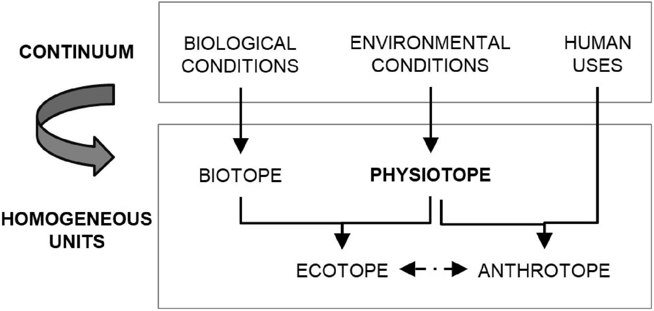
Figure 1. Conceptual framework for scaling the continuum range of environmental, biological and human conditions into homogeneous units in complex nature-human systems.

This conceptual framework (Figure 1) agrees with the recent advancements in the decision support tools for ecosystem-based management, which include the assessment of cumulative impacts of multiple pressures on multiple ecosystem components (Holsman et al., 2016). Many of the approaches used to assess these cumulative impacts are similar to the one developed by Halpern et al. (2008) for the global-scale assessment of human impacts on marine environment (Korpinen and Andersen, 2016). However, their application at a smaller scale such as the estuary require adapting the spatial resolution of the input data and the methods (Borja et al., 2016). Multiple pressures in the estuary includes environmental, ecological and anthropogenic pressures that can be spatially explicit characterized through physiotope, biotope and anthrotope maps, respectively. Likewise, the target ecosystem component of the assessment can be characterized by the biotope-ecotope. In turn, this holistic characterization is required at different spatial scales according to the different meaningful social and ecological scales recognized within the estuary. Regarding the assessment methodologies, those approaches classified as a qualitative or semi-quantitative ecosystem risk assessment of multiple stressor on independent biological subjects (Level 2, Class 2 sensu Holsman et al., 2016), like the one proposed by Halpern et al. (2008), allow optimizing the effort and data/knowledge requirements with the obtained results and response time.

In the context of this study, the basic spatial unit in socio-ecological systems is delimited by the physiotope, which acts as a surrogate for the distribution patterns of biota and human uses. It is described based on those physical and chemical properties of the environment that determine the spatial patterns of biota (i.e., biotope). In this regard, the number and nature of the specific variables that allow explaining the distribution of species and the ecological functioning of the estuary at different spatial scales is the main unsolved question. In general terms, physiotopes in estuaries can be described through a reduced number of variables, mainly those related to salinity, depth, current velocity, sediment composition and water renovation (Ysebaert et al., 2002; Bouma et al., 2006; Lee et al., 2007; Foti et al., 2012).

Therefore, this paper aims at developing a multiscale spatial classification model for estuaries by clearly representing the distribution of environmental components and synthesizing data on the biological components and the anthropogenic drivers of ecological change in an estuary. The hierarchical methodology and resulting maps provide flexible tools for conservation, ecosystems-based management, spatial planning, education, and research.

Materials and Methods

Study Area

The methodology to identify homogenous units within estuaries was applied in the Marismas de Santoña (north of Spain) (Figure 2). This estuary is characterized by soft bottoms, large intertidal areas (67% of the total estuarine area), meso-tidal conditions (2.8 m of median tidal range) and irregular hydrological regimes (16 m³/s of mean water flow of the Asón river) that hinder water stratification. It is also one of the largest estuaries in southern Bay of Biscay (18 km²) with a high biological and environmental diversity. It houses important subtidal meadows of Zostera marina (Linnaeus, 1832) and intertidal meadows of Zostera noltei (Hornemann, 1832). This ecosystem is protected by different legal figures: Natural Park (local legislation), Site of Community Importance (SCI, European Directive 92/43/CEE), Special Protection Area for Birds (SPA, European Directive 2009/147/CE) and RAMSAR site. Although this estuary has a good ecosystem health, it is exposed to anthropogenic pressures mainly related to land reclamation, urban/industrial discharges and fishing harbor activities.

FIGURE 2

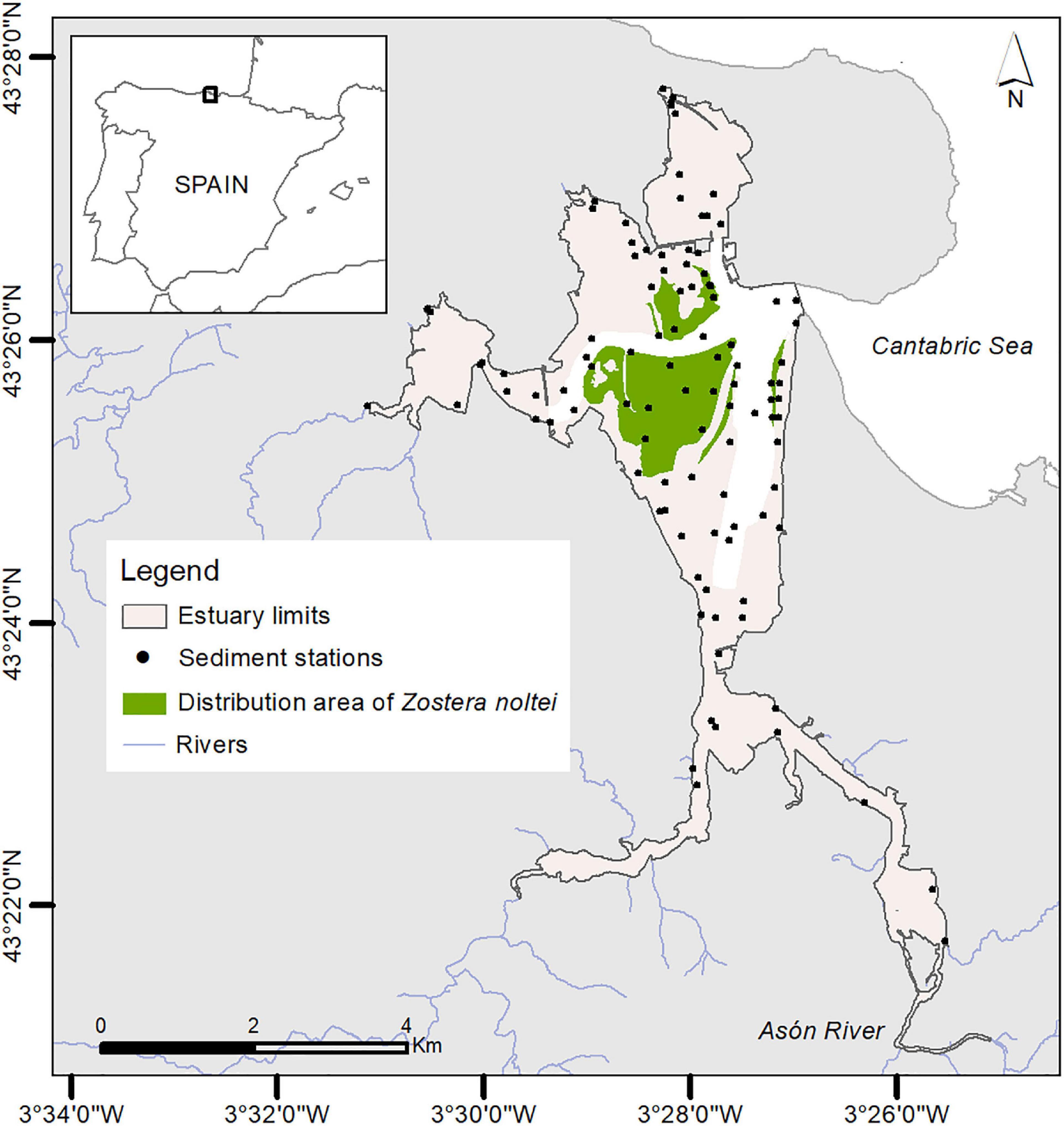
Figure 2. Study site: location of Santoña estuary in the northern Spain. Spatial distribution of grain size sediment samples and distribution of seagrass meadows of Zostera noltei in 2005.

Data on sediment composition was available between 1993 and 2012 for 94 stations. Data on depth, river flow, tide, water level, shear stress and salinity were obtained from Galván et al. (2016). The distribution of intertidal seagrasses, specifically dwarf eelgrass (Zostera noltei), was obtained from a field survey (2005).

Environmental Dimension: Physiotope

The approach to establish a classification system to identify representative physiotopes in the estuary encompasses four main steps: (i) selection of abiotic variables; (ii) characterization of abiotic variables with a high spatial and/or temporal resolution; (iii) classification of abiotic variables based on thresholds; and (iv) hierarchical integration of abiotic variables to obtain physiotopes at different spatial scales.

Five variables were included in the classification methodology: substratum, bathymetry, salinity, water velocity, and water renewal. Each one was characterized using one or more subvariables representative of the biological variability associated to different spatial scales, and then classified based on specific criteria and thresholds (Table 1).

TABLE 1

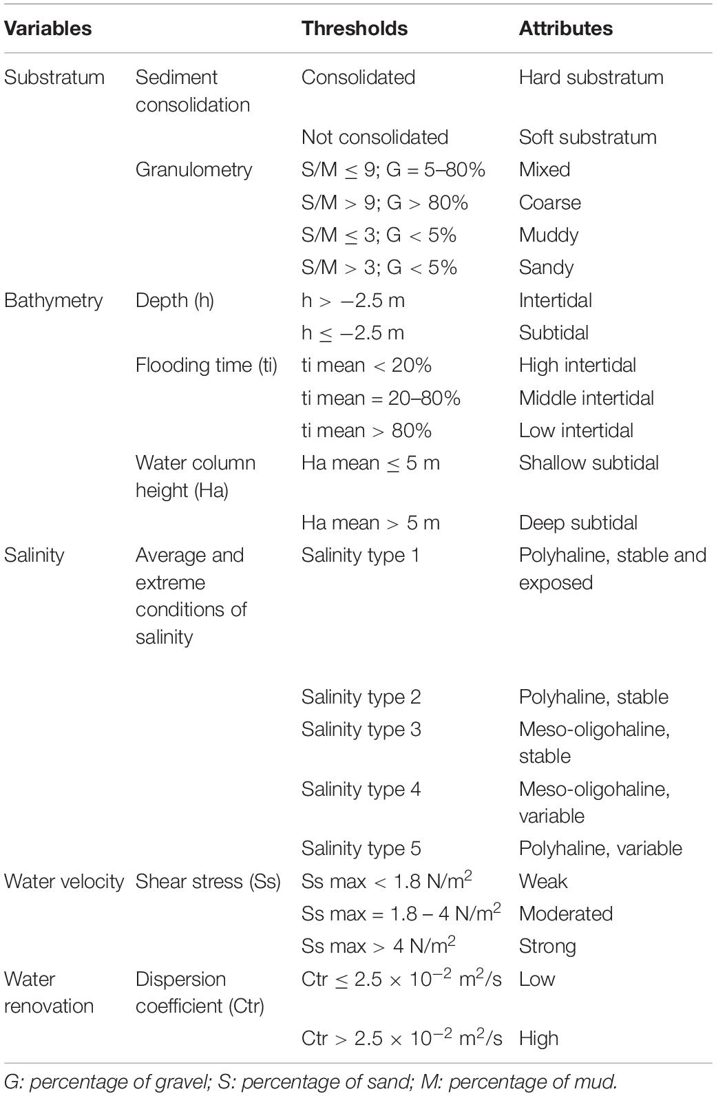
Table 1. Variables and classes (thresholds and attributes) included in the classification system of the estuarine physiotopes.

The first variable, substratum, was described grouping sediment into hard or soft sediment, and granulometry, as the proportion of gravel (>2,000 μm), sand (63–2,000 μm) and mud (<63 μm). These sedimentary fractions were interpolated at a higher spatial resolution with the geostatistical method of cokriging (Verfaillie et al., 2006; Jerosch, 2012). The bathymetry map was used as a cokriging parameter. A modification of the Folk (1954) and UKSeaMap (Long, 2006) classification system was then applied to the obtained multi-parametric sediment type map (Table 1).

The second variable, bathymetry, was represented by three subvariables: depth, duration of flooding and water column height. Regarding depth, the estuary was divided into subtidal and intertidal zones according to the lowest water level registered in the study area (i.e., 2.5 m under the Mean Sea Level) (Table 1). Flooding time and water column height were estimated from the reconstructed water level variations over 15 years using the methodology described by Galván et al. (2016). Flooding time in intertidal areas was calculated as the inter-annual mean inundation time (in hours). The intertidal was classified into three categories based on two thresholds: 20 and 80% of the time covered by water, respectively (Pennings and Callaway, 1992; Costa et al., 2003; Table 1). Likewise, water column height in subtidal areas was calculated as the mean inter-annual value. A threshold value of 5 m of water column height was established because it corresponds with the limit of penetration of 10% of the solar irradiance in the water surface in the study area (Duarte, 1991; Greve and Binzer, 2004; Guinda et al., 2012; Table 1).

The third variable, salinity, was described based on eight different subvariables that give information about average and extreme conditions (Galván et al., 2016). All of them were objectively integrated using statistical techniques in order to identify five salinity types (Table 1).

The fourth variable, water velocity, was represented by bottom shear stress and it was characterized as the mean inter-annual value of the annual maximum shear stress in a reconstructed series of 15 consecutive years (methodology described by Galván et al., 2016). Two threshold values of 1.8 and 4 N/m², respectively, allowed classifying the estuary into three categories (Coltman et al., 2008; Table 1).

Lastly, we used the dispersion coefficient as a surrogate of water renovation or flushing time (an inverse relationship), its spatial variability being obtained using a bidimensional numerical model of transport (Revilla et al., 1995). For this variable, we established a threshold value of 0.025 m²/s to differentiate high and low water renovation zones (Gómez et al., 2014; Table 1).

As a result of applying the previously described steps, we obtained an independent layer for each physical-chemical variable with information about the estuarine spatial distribution of the different classes recognized within variables (Table 1). Based on these layers, the physiotope was calculated in each pixel at a specific level of detail by spatial overlapping of all the variable layers corresponding to such level of detail (Figure 3). A different physiotope (P) was assigned for each unique combination of classes of the different variables, according to the equation P_kj = ⋃_i∈k V_ij, where V is the physical-chemical variable i (composed of the classes defined in Table 1) included within the level of detail k (Figure 3) in the pixel j. This calculation was done in ArcGIS 10.1 with the Combine tool.

FIGURE 3

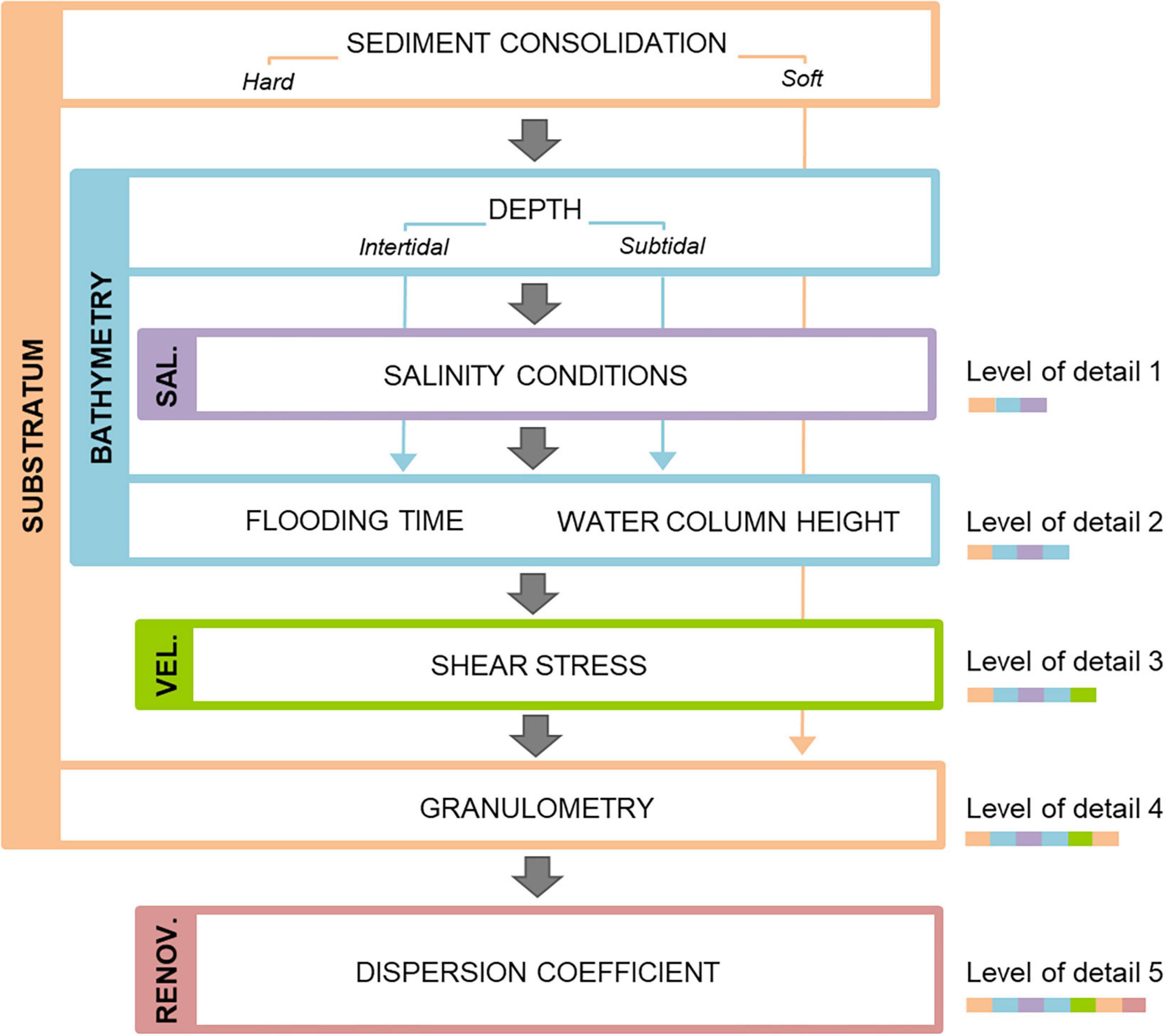
Figure 3. Scheme of the hierarchical integration of abiotic variables and subvariables to obtain the estuarine physiotopes at five scales or levels of detail.

Biological Dimension: Biotope and Ecotope

The biotope of Z. noltei at the Santoña estuary was estimated using the maximum entropy species distribution modeling (Maxent) (Phillips et al., 2006) and a set of environmental predictors (Table 1) in the study area. Most of the Maxent settings were left at their default values when constructing the model. Ten percent of the records of presence were randomly selected avoiding spatial autocorrelation and used to train the model, while the remaining 90% were withheld to test it. We select the most appropriate regularization parameter (1, 2, 3, 5, 10, 15, and 20) for Z. noltei based on AUC (Area Under the Curve) and omission rate.

The suitability (in terms of probability of presence) map modeled was converted into a binary map that differentiated between suitable and unsuitable regions for the development of Z. noltei meadows. To distinguish between both, the best performing threshold value was calculated to balance training omission, predicted area and threshold value.

Finally, the ecotope was calculated in each pixel by spatial overlapping of both physiotope and biotope and assigning a different ecotope for each unique combination of biotope and physiotope classes. Therefore, the ecotope (E) was calculated according to the equation E_j = B_ij ∪ P_kj, where B is the biotope of species i (in this case, only Z. noltei) in pixel j, and P is the physiotope class at the level of detail k in the pixel j. This calculation was done in ArcGIS 10.1 with the Combine tool.

Human Dimension: Anthrotope

The main human pressures in the target estuary were classified into eight categories: hydro-morphological alterations (i.e., tidal mill, dikes, roads, bridges), non-native species, dredging works, tourism (i.e., recreation trails) and diffuse/point organic/non-organic discharges (Supplementary Table S1).

First, the affected area of all the pressure sources was delimited based on different criteria: (i) a buffer of 500 m for non-native species and dredging works; (ii) a buffer of 1,000 m for residual and industrial discharges into the estuary; (iii) a variable buffer, proportional (factor = 1.5) to the length of the dikes and tidal mills; (iv) a buffer of 10 m at both sides of roads and bridges; and (v) the area covered by recreation trails. Then, the magnitude of each pressure source was calculated using a ranking scale of three points (i.e., low, moderate, and high magnitude). The methodology and criteria applied to assign the ranking scale to each anthropogenic pressures are described in the Supplementary Data (Supplementary Method S1). Next, the extension and magnitude of each pressure category was characterized as the maximum value of all pressure sources belonging to such category in each pixel.

Finally, the anthrotope was estimated as the pressure footprint in each spatially independent unit of the physiotope map (Fp) according to the equation $F_P=\left({\sum }_{j=1}^{\mathrm{j}=\mathrm{N}}{\sum }_{i=1}^{\mathrm{i}=\mathrm{n}}{M}_i\right)/N$ (Halpern et al., 2008), where M is the magnitude of pressure i in pixel j, and N is the number of pixels per independent unit of the physiotope map. The interaction between the anthrotope and the ecotope was assessed as the potential impact of accumulated pressures on Z. noltei (Ic) based on the equation $I_C=\left({\sum }_{i=1}^{\mathrm{i}=\mathrm{n}}{M}_i\times S_i\right)/N$, where S is the impact weight score for seagrasses to anthropogenic pressures of type i (Halpern et al., 2008; Supplementary Table S1).

Results

Physiotope

All abiotic variables included in the physiotope model showed a strong variability within the estuary (Supplementary Figures S1, S2). In Santoña, subtidal areas mainly consist of deeper channels, which are characterized by high values of shear stress and sandy sediments. Conversely, intertidal areas are characterized by sediments rich in mud grain size, especially in areas under the direct influence of river inputs. A continuous gradient from the river to the sea was observed for salinity and a gradient from land to water was observed for flooding times.

The integration of the regions delimited for each environmental variable showed a mosaic of physiotopes (Figure 4): 10, 23, 57, 77, and 93 physiotopes from level of detail 1 to 5, respectively. The highest diversity of physiotopes was detected in the large central zone where the largest intertidal flats and channels of the estuary are located. On the other hand, the lowest richness of physiotopes was linked to areas near the river.

FIGURE 4

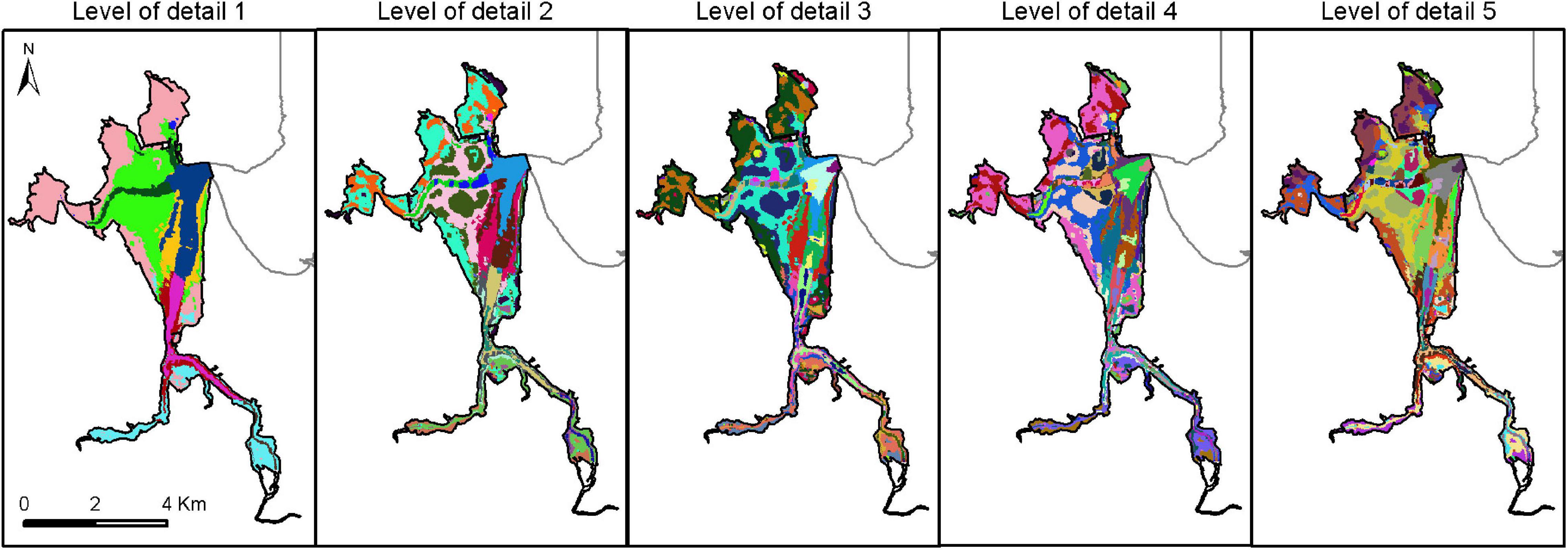
Figure 4. Spatial distribution of physiotopes in the Santoña estuary at five scales (10, 23, 57, 77 y 93 biotopes from level 1 to level 5, respectively). Different colors represent different physiotopes within each level of detail.

Biotope and Ecotope of Zostera noltei

The most important variables in the obtained optimized model (regularization multiplier equal to 10, Supplementary Figure S3) were the percentage of mud in the sediment (27%), frequency of drought events on salinity (19.4%), water renovation (16.7%), and variations in salinity (12%). The highest values of environmental suitability for Z. noltei were observed in areas near the mouth of the estuary and close to the main channels (Supplementary Figure S4). Based on a logistic threshold value of 0.1013, a total surface of 4.78 km² was identified as the potential distribution area of the species in the estuary. The relatively large range of environmental conditions within the biotope of Z. noltei encompassed different physiotopes, giving rise to a mosaic of ecotopes: from 4 ecotopes in level 1 to 28 in level 5 (Figure 5).

FIGURE 5

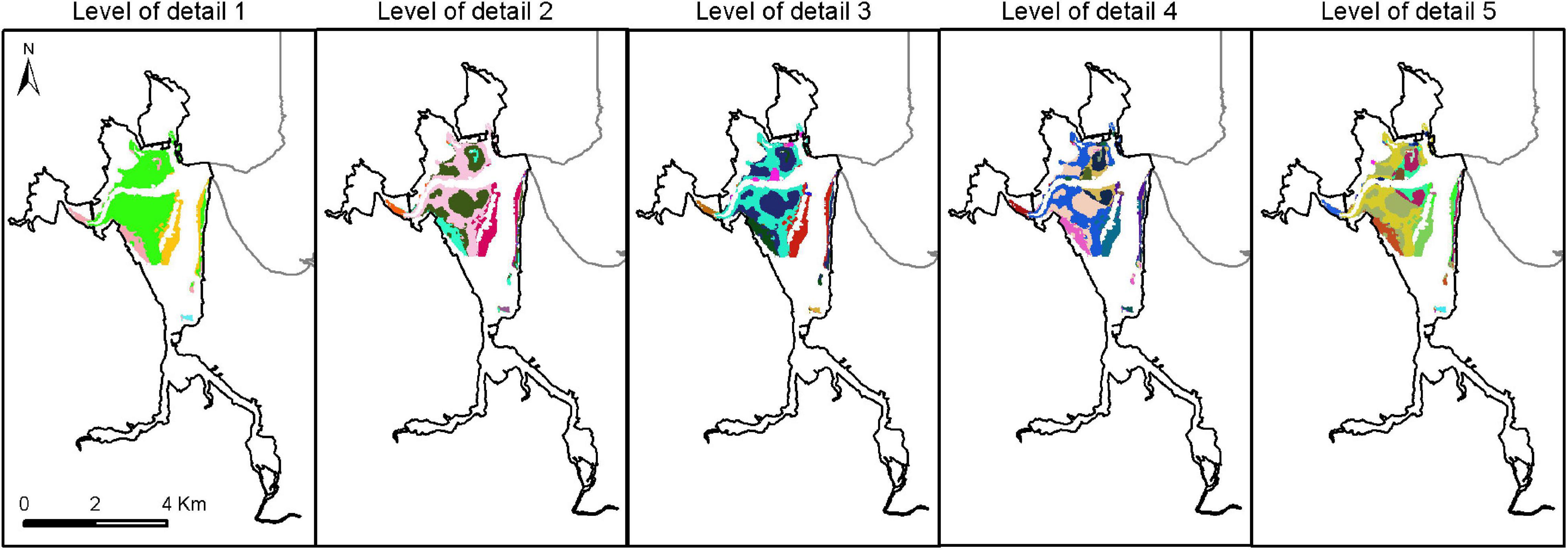
Figure 5. Spatial distribution of the ecotopes of Zostera noltei in the Santoña estuary at five scales (4, 8, 17, 25 y 28 ecotopes from level 1 to level 5, respectively). Different colors represent different ecotopes within each level of detail.

Anthrotope

The map of cumulative footprints highlighted the widespread distribution of all the pressure categories (Supplementary Figures S6, S7). Most physiotopes were affected by multiple stressors, but the relative importance of different pressure sources varied among them. Hydro-morphological alterations showed the largest and broadest contribution to the footprint in the estuary, though locally, the contribution of non-organic discharges was higher. The mouth of the estuary had the lowest footprint of accumulated pressures, while the higher footprint was concentrated around urban and industrial areas.

Lower levels of detail attenuate the lowest and highest footprint values and scores of cumulative impact on Z. noltei (Figure 6). The highest probability of occurrence of Z. noltei were observed in those anthrotopes with a lower cumulative impact score (<9) and, specifically, with a low or null impact of non-organic discharges. Those areas near the sand spit and/or urban/industrial areas were exposed to the highest cumulative impact scores (>17), indicative of locally high impacts linked to non-organic discharges.

FIGURE 6

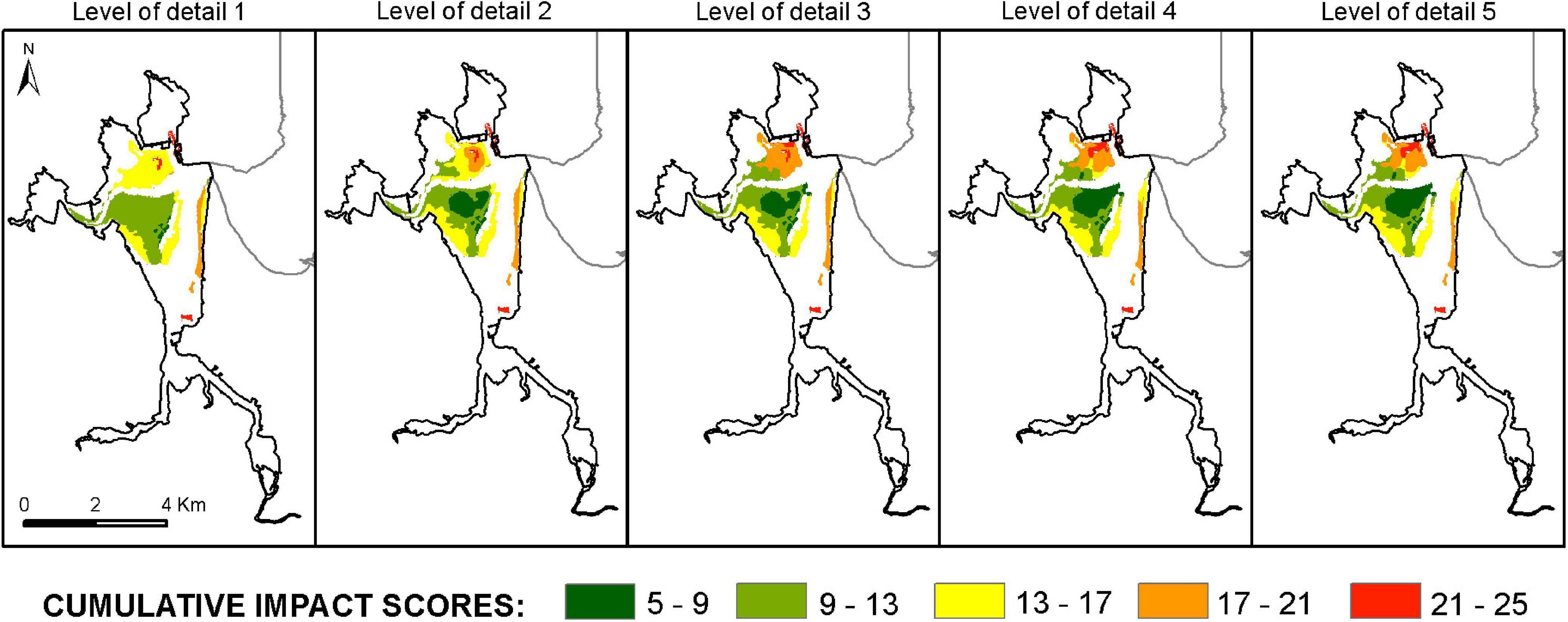
Figure 6. Cumulative impact scores, for all the pressure types used in this analysis, per spatially independent unit of the ecotope map of Zostera noltei at five spatial scales.

Discussion

Multiscale classification models provide a holistic view of estuarine socio-ecological systems avoiding information losses in any of the relevant parts of the system. As opposed to conventional and sectorial approaches of limited uses, the proposed methodology combined biological, environmental and human dimensions in manageable units that can be directly applicable for a wide range of purposes such as ecosystem-based management and conservation (Guarinello et al., 2010; de Jonge et al., 2012). Besides, this classification system can capture the different spatial scales at which ecological processes and human pressures operate within ecosystems, using a versatile hierarchical approach.

An important advance of this approach with respect to existing methods is related with the scale of the application at an estuarine level. A high number of examples are available for the marine environment and broad-spatial scales (Holsman et al., 2016), but few studies have been developed in estuaries (Lonsdale et al., 2018). Improvements of the methods were needed for representing the social complexity (estuaries are one of the most pressured ecosystems) and ecological complexity (estuaries are highly dynamic transitional ecosystems) of estuaries. Specifically, a detailed methodology for characterizing the extent and magnitude of different types of pressures within the estuary was developed in this study (Elliott et al., 2014; Stelzenmüller et al., 2018). Accordingly, the cumulative pressure assessment method developed by Halpern et al. (2008) for the marine environment was adapted here to be applied using the anthrotope map and the ecotope map. Unlike Halpern et al. (2008) and most of the current existing tools, instead of using presence or absence data of target species, it is used the ecotope that provides explicit additional information on the range of environmental characteristics in which such species is present. This is an important point in estuaries because the need to account for the environmental variability in pressure assessment increases at small scales (Borja et al., 2016). Thus future scientific research should be focused on developing weighing scores (sensu Halpern et al., 2008) sensitive to such local factors.

In the proposed methodology, the scale-dependent within-estuary complexity is represented by physiotopes, biotopes, ecotopes and anthrotopes at five nested spatial scales, providing a gradually increasing description of biological and social processes. In turn, this methodology is also susceptible to being nested within other classification systems that operate at a regional scale. Hydrological, morphological, and climatic factors determine these large differences among estuaries (Galván et al., 2010). However, this challenge of incorporating the within-estuary and inter-estuary variability into a single, universal estuarine classification system remains a challenge for the scientific community that should be addressed in the future.

The availability of information is one of the main limitations in the use and application of this type of mapping methodologies, which generally have high data requirements. In this case, the hierarchical approach of the methodology has the advantage of adapting the scale of the study to, among other things, data availability. The higher the level of detail, the more data needed. To meet such increasing data requirements, in our case, complex interpolation techniques and numerical models could be used to distinguish among the various socio-ecological units nested in the estuary at finer-scales. Both techniques allowed characterizing estuarine environmental conditions at high spatial and temporal resolutions, while reducing the costs and efforts in comparison with field surveys and laboratory work (Diaz et al., 2004; Ducrotoy, 2010). Nevertheless, several assumptions and limitations are inherent to the application of these techniques. Specifically, in this study, the variables used for the salinity characterization did not allow detecting small changes in the physiotopes over periods shorter than a year.

There are two other major limitations in this study that could be addressed in future research. The first is that indirect interactions between the human activities and the ecology have not been taken into account in the model (e.g., pressure on predators of target species could reduce density of predators and indirectly increase density of target species). Addressing this task would require an extensive knowledge of the ecology of the target species (e.g., food chain or biotic interactions such as facilitation or competition) (Holsman et al., 2016), in addition to the characterization of the distribution area of interacting species (i.e., their biotope). Therefore, a multispecies biotope map is needed, which can be addressed by using techniques such as joint species distribution models (Wilkinson et al., 2021) or combined approaches (Pellisier et al., 2013). In this context, the role of the present approach is identifying vulnerable components that can be further analyzed considering indirect interactions between human activities and target species through impacts on interacting species. The second limitation is that the proposed approach is a one-way coupled socio-ecological model, which limits the type of questions that the model can answer (Kasperski et al., 2021). Here, outputs from anthrotope model are inputs into the ecotope model with no feedback to the first model. A two-way couple model can be potentially developed based on the physiotope, biotope, ecotope and anthrotope maps. Nevertheless, new linkages between these maps and indicators should be developed and incorporated into the model. For example, variables that link natural and human components, such as ecosystem services, or human variables, such as structures of multilevel governance. Dynamics of human-nature systems are influenced by government policies and, in the context of the present study, by the national and international legislative framework that has given rise to many types of existing estuarine management plans. However, boundaries of management systems and governance mechanisms have not been integrated in the present approach. In the future, they could be incorporated within the model as new additional maps that overlap with the ecotope and anthrotope maps (Lonsdale et al., 2015, 2018), but a further research about how to integrate specific requirements of management plans in this model is needed.

Biotope delimitation is a key point of the methodology that is open to discussion because of its implications in results interpretation and scope. Firstly, the question of how to define the distribution area of the target species, either as a potential or a realized area, must be considered. Secondly, there is a wide range of tools available to define the distribution area, from field data to remote sensing techniques and modeling. Several correlative techniques such as Maxent (Phillips et al., 2006), which was mainly used in this study to delimitate the potential distribution area of Z. noltei, allow predicting suitable environments for species establishment and survival. Other approaches with more data requirements, such as mechanistic and hybrid models, integrate hypotheses about niche, dispersal abilities and biotic interactions that provide more detailed information about patterns of species and other related properties (e.g., productivity or population dynamics). A rigorous exploration of the capabilities of both correlative and mechanistic approaches in the framework of the nested classification system should be carried out. In any case, all these approaches are suitable to be integrated within the proposed ecotope model.

Differences between the realized and potential biotope of Z. noltei can be mainly explained by biotic interactions, that were not taken into account in this study, or by human pressures. In this regard, an innovation of the classification model is that it provides a practical focus to combine, at the same spatial scale, both bio-physical information and human pressures causing impacts on the ecosystem. Integrating both ecotope and anthrotope maps allows an assessment of the ecosystem’s vulnerability and its spatial distribution, which is essential to understand how estuaries are affected by human activities. The anthrotope provides a systematic, transparent, and replicable assessment of the multiple threats that affect ecosystems at different scales relevant to managers. These maps are basic for the design of productive management and conservation actions by identifying key threats or priority ecotopes. Likewise, they can be used to identify areas and species where a better management of human activities could render a higher return on management/conservation investments (Halpern et al., 2008). The future will inevitably be aimed at developing further studies and experimental works to quantify ranges of tolerance of species against different pressure types under varying environmental conditions. New empirical information will allow improving anthrotope maps and impact assessment through the enhancement of predictive capacities, and increasing the wide variety of applications of this type of models.

A sustainable management of estuaries depends on an exhaustive diagnostic procedure able to generate a holistic understanding of the system. In this sense, the interdisciplinary research developed in this study combines natural (ecotope) and human (anthrotope) data to operationalize a spatially explicit analysis of estuaries at different levels of detail and to bridge the gap between social and ecological sciences. Therefore, the resulting nested socio-ecological maps are a powerful spatial planning instrument essential for the design and implementation of estuarine governance, conservation policies and ecosystem-based management approaches. They allow exploring effects of environmental and social changes, such as climate change or transitions to a green economy, on the estuarine ecosystem and their capacity to provide goods and services. In fact, ecosystem services are themselves the expression of complex interactions between the three components included in the classification system: biophysical context (e.g., landscape heterogeneity, biodiversity composition), ecological processes, and human interventions (Bennett et al., 2015). In this way, the proposed methodology can be adapted to understand and manage the trends observed in ecosystem service provision, minimizing their potential future reduced supply.

Data Availability Statement

The datasets presented in this study can be found in online repositories. The names of the repository/repositories and accession number(s) can be found below: Figshare with the identifier http://doi.org/10.6084/m9.figshare.14339312.

Author Contributions

All authors listed have made a substantial, direct and intellectual contribution to the work, and approved it for publication.

Funding

This study was funded through an F.P.U. (“Formación de Profesorado Universitario”) grant and the mobility grant “José Castillejo” of the Spanish Ministry of Education to CG. This research was part of the ECOTOPO project (RTI2018-096409-B-I00) financially supported by the Spanish Ministry of Science and Innovation through the National Plan for Scientific Research.

Conflict of Interest

The authors declare that the research was conducted in the absence of any commercial or financial relationships that could be construed as a potential conflict of interest.

Publisher’s Note

All claims expressed in this article are solely those of the authors and do not necessarily represent those of their affiliated organizations, or those of the publisher, the editors and the reviewers. Any product that may be evaluated in this article, or claim that may be made by its manufacturer, is not guaranteed or endorsed by the publisher.

Supplementary Material

The Supplementary Material for this article can be found online at: https://www.frontiersin.org/articles/10.3389/fmars.2021.730762/full#supplementary-material

References

Bennett, E. M., Cramer, W., Begossi, A., Cundill, G., Díaz, S., Egoh, B. N., et al. (2015). Linking biodiversity, ecosystem services, and human well-being: three challenges for designing research for sustainability. Curr. Opin. Environ. Sustain. 14, 76–85. doi: 10.1016/j.cosust.2015.03.007

CrossRef Full Text | Google Scholar

Borja, A., Elliott, M., Andersen, J. H., Berg, T., Carstensen, J., Halpern, B. S., et al. (2016). Overview of integrative assessment of marine systems: the ecosystem approach in practice. Front. Mar. Sci. 3:20. doi: 10.3389/fmars.2016.00020

CrossRef Full Text | Google Scholar

Bouma, H., de Jong, D. J., Twisk, F., and Wolfstein, K. (2006). Ecotope System for Saline Waters (ZES.1), Ministry of Transport, Public Works and Water Management. Middelburg: National Institute for Coastal and Marine Management, 135.

Google Scholar

Coltman, N., Golding, N., and Verling, E. (2008). “Developing a broadscale predictive EUNIS habitat map for the MESH study area,” in Proceeding of the Joint Nature Conservation Committee, 16.

Google Scholar

Costa, C. S. B., Marangoni, J. C., and Azevedo, A. M. G. (2003). Plant zonation in irregularly flooded salt marshes: relative importance of stress tolerance and biological interactions. J. Ecol. 91, 951–965. doi: 10.1046/j.1365-2745.2003.00821.x

CrossRef Full Text | Google Scholar

Davies, C. E., and Moss, D. (2002). EUNIS Habitat Classification, Centre for Ecology and Hydrology. Huntingdon: Natural Environment Research Council, 108.

Google Scholar

de Jonge, V., Pinto, R., and Turner, R. K. (2012). Integrating ecological, economic and social aspects to generate useful management information under the EU Directives’ ‘ecosystem approach’. Ocean Coast. Manag. 68, 169–188. doi: 10.1016/j.ocecoaman.2012.05.017

CrossRef Full Text | Google Scholar

Diaz, R. J., Solan, M., and Valente, R. M. (2004). A review of approaches for classifying benthic habitats and evaluating habitat quality. J. Environ. Manage. 73, 165–181. doi: 10.1016/j.jenvman.2004.06.004

PubMed Abstract | CrossRef Full Text | Google Scholar

Duarte, C. M. (1991). Seagrass depth limits. Aquat. Bot. 40, 363–377. doi: 10.1016/0304-3770(91)90081-f

CrossRef Full Text | Google Scholar

Ducrotoy, J. P. (2010). The use of biotopes in assessing the environmental quality of tidal estuaries in Europe. Estuar. Coast. Shelf Sci. 86, 317–321. doi: 10.1016/j.ecss.2009.05.023

CrossRef Full Text | Google Scholar

Elliott, M., Cutts, N. D., and Trono, A. (2014). A typology of marine and estuarine hazards and risks as vectorsof change: a review for vulnerable coasts and their management. Ocean Coastal Manag. 93, 88–99. doi: 10.1016/j.ocecoaman.2014.03.014

CrossRef Full Text | Google Scholar

Folk, R. L. (1954). The distinction between grain size and mineral composition in sedimentary rock nomenclature. J. Geol. 62, 344–359. doi: 10.1086/626171

CrossRef Full Text | Google Scholar

Foti, R., del Jesús, M., Rinaldo, A., and Rodríguez-Iturbe, I. (2012). Hydroperiod regime controls the organization of plant species in wetlands. PNAS 109, 19596–19600. doi: 10.1073/pnas.1218056109

PubMed Abstract | CrossRef Full Text | Google Scholar

Galván, C., Juanes, J. A., and Puente, A. (2010). Ecological classification of European transitional waters in the North-East Atlantic eco-region. Estuar. Coast. Shelf Sci. 87, 442–450. doi: 10.1016/j.ecss.2010.01.026

CrossRef Full Text | Google Scholar

Galván, C., Puente, A., Castanedo, S., and Juanes, J. A. (2016). Average vs. extreme salinity conditions: do the equally affect the distribution of macroinvertebrates in estuarine environments? Limnol. Oceanogr. 61, 984–1000. doi: 10.1002/lno.10267

CrossRef Full Text | Google Scholar

Gómez, A. G., Juanes, J. A., Ondiviela, B., and Revilla, J. A. (2014). Assessment of susceptibility to pollution in littoral waters using the concept of recovery time. Mar. Pollut. Bull. 81, 140–148. doi: 10.1016/j.marpolbul.2014.02.004

PubMed Abstract | CrossRef Full Text | Google Scholar

Greve, T. M., and Binzer, T. (2004). “Which factors regulate seagrass growth and distribution?” in European Seagrasses: An Introduction to Monitoring and Management, eds C. D. J. Borum, D. Krause-Jensen, and T. M. Greve (The M&MS project), 19–23.

Google Scholar

Guarinello, M. L., Shumchenia, E. J., and King, J. W. (2010). Marine habitat classification for ecosystem-based management: a proposed hierarchical framework. Environ. Manage. 45, 793–806. doi: 10.1007/s00267-010-9430-5

PubMed Abstract | CrossRef Full Text | Google Scholar

Guinda, X., Juanes, J. A., Puente, A., and Echavarri-Erasun, B. (2012). Spatial distribution pattern analysis of subtidal macroalgae assemblages by a non-destructive rapid assessment. J. Sea Res. 67, 34–43. doi: 10.1016/j.seares.2011.09.006

CrossRef Full Text | Google Scholar

Halpern, B. S., Walbridge, S., Selkoe, K. A., Kappel, C. V., Micheli, F., D’Agrosa, C., et al. (2008). A global map of human impact on marine ecosystems. Science 319, 948–952. doi: 10.1126/science.1149345

PubMed Abstract | CrossRef Full Text | Google Scholar

Holsman, K., Samhouri, J., Cook, G., Hazen, E., Olsen, E., Dillard, M., et al. (2016). An ecosystem-based approach to marine risk assessment. Ecosyst. Health Sustainabil. 3, 1–16. doi: 10.1002/ehs2.1256

CrossRef Full Text | Google Scholar

Hornemann, J. W. (1832). Flora Danica Fasciculus Trigesmus Quintus. Copenhagen: pls MMXLI-MMLX.

Google Scholar

Jerosch, K. (2012). Geostatistical mapping and spatial variability of surficial sediment types on the beaufort shelf based on grain size data. J. Mar. Syst. 127, 5–13. doi: 10.1016/j.jmarsys.2012.02.013

CrossRef Full Text | Google Scholar

Kasperski, S., DePiper, G. S., Haynie, A. C., Blake, S., Colburn, L. L., Freitag, A., et al. (2021). Assessing the state of coupled social-ecological modeling in support of ecosystem based fisheries management in the united states. Front. Mar. Sci. 8:631400. doi: 10.3389/fmars.2021.631400

CrossRef Full Text | Google Scholar

Korpinen, S., and Andersen, J. H. (2016). A global review of cumulative pressure and impact assessments in marine environments. Front. Mar. Sci. 3:153. doi: 10.3389/fmars.2016.00153

CrossRef Full Text | Google Scholar

Lee, K.-S., Park, S. R., and Kim, Y. K. (2007). Effects of irradiance, temperature, and nutrients on growth dynamics of seagrasses: a review. J. Exp. Mar. Biol. Ecol. 350, 144–175. doi: 10.1016/j.jembe.2007.06.016

CrossRef Full Text | Google Scholar

Linnaeus, C. (1753). Species Plantarum, Exhibentes Plantas Rite Cognitas ad Genera Relatas cum Differentiis Specificis, Nominibus Trivialibus, Synonymis Selectis, Locis Natalibus, Secundum Systema Sexuale Digestas, Vol. 2. Stockholm: Impensis Laurentii Salvii.

Google Scholar

Long, D. (2006). BGS Detailed Explanation of Seabed Sediment Modified Folk Classification. Peterborough, UK: MESH (Mapping European Seabed Habitats).

Google Scholar

Lonsdale, J., Nicholsona, R., Westona, K., Elliott, M., Birchenougha, A., and Sühringa, R. (2018). A user’s guide to coping with estuarine management bureaucracy: an estuarine planning support system (EPSS) tool. Mar. Pollut. Bull. 137, 463–477. doi: 10.1016/j.marpolbul.2017.12.032

PubMed Abstract | CrossRef Full Text | Google Scholar

Lonsdale, J.-A., Weston, K., Barnard, S., Boyes, S. J., and Elliott, M. (2015). Integrating management tools and concepts to develop an estuarineplanning support system: a case study of the Humber Estuary, Eastern England. Mar. Pollut. Bull. 100, 393–405. doi: 10.1016/j.marpolbul.2015.08.017

PubMed Abstract | CrossRef Full Text | Google Scholar

Madden, C. J., Grossman, D. H., and Goodin, K. L. (2010). Coastal and Marine Ecological Classification Standard Version 3.1.

Google Scholar

Mount, R., Bricher, P., and Newton, J. (2007). National Intertidal/Subtidal Benthic (NISB) Habitat Classification Scheme. Version 1.0.

Google Scholar

Pellisier, L., Rohr, R. P., Ndiribe, C., Pradervand, J. N., Salamin, N., Guisan, A., et al. (2013). Combining food web and species distribution models for improved community projections. Ecol. Evol. 3, 4572–4583. doi: 10.1002/ece3.843

PubMed Abstract | CrossRef Full Text | Google Scholar

Pennings, S. C., and Callaway, R. M. (1992). Salt marsh plant zonation: the relative importance of competition and physical factors. Ecology 73, 681–690. doi: 10.2307/1940774

CrossRef Full Text | Google Scholar

Phillips, S. J., Anderson, R. P., and Schapire, R. E. (2006). Maximum entropy modeling of species geographic distributions. Ecol. Model. 190, 231–259. doi: 10.1016/j.ecolmodel.2005.03.026

CrossRef Full Text | Google Scholar

Revilla, J. A., Koev, K. N., Díaz, R., Álvarez, C., and Roldán, A. (1995). Methods for studying dissolved oxygen levels in coastal and estuarine waters receiving combined sewer overflows. Water Sci. Technol. 32, 95–103. doi: 10.2166/wst.1995.0081

CrossRef Full Text | Google Scholar

Stelzenmüller, V., Coll, M., Mazaris, A. D., Giakoumi, D. S., Katsanevakis, S., Portman, M. E., et al. (2018). A risk-based approach to cumulative effect assessments for marine management. Sci. Total Environ. 632, 1132–1140. doi: 10.1016/j.scitotenv.2017.08.289

PubMed Abstract | CrossRef Full Text | Google Scholar

Verfaillie, E., Van Meirvenne, M., and Van Lancker, V. (2006). Multivariate geostatistics for the predictive modeling of the surficial sand distribution in shelf seas. Cont. Shelf Res. 26, 2454–2468. doi: 10.1016/j.csr.2006.07.028

CrossRef Full Text | Google Scholar

Wilkinson, D. P., Golding, N., Guillera-Arroita, G., Tingley, R., and McCarthy, M. A. (2021). Defining and evaluating predictions of joint species distribution models. Methods Ecol. Evol. 12, 394–404. doi: 10.1111/2041-210X.13518

CrossRef Full Text | Google Scholar

Ysebaert, T., Meire, P., Herman, P. M. J., and Verbeek, H. (2002). Macrobenthic species response surfaces along estuarine gradients: prediction by logistic regression. Mar. Ecol. Prog. Ser. 225, 79–95. doi: 10.3354/meps225079

CrossRef Full Text | Google Scholar