The Gulf of St. Lawrence Biogeochemical Model: A Modelling Tool for Fisheries and Ocean Management

Introduction

The Gulf of St. Lawrence (GSL) is a large semi-enclosed sea (covering an area of about 240000 km²) located in eastern Canada that connects to the northwest Atlantic through the relatively shallow Strait of Belle Isle (50–80 m; Bailey, 1958) and the deep (480 m) Cabot Strait (Figure 1). Waters flowing in through the Strait of Belle Isle are mostly of Arctic origin [see Figure 1 of Lavoie et al. (2019)], while waters entering at Cabot Strait are a mixture of cold water from the Labrador Current and warmer North Atlantic Central Water. The GSL is characterized by deep channels (Laurentian, Esquiman, and Anticosti) bordered by relatively narrow shelves, except for the Magdalen Shallows, a vast shelf that covers most of the southern GSL with an average depth of 60–65 m. The GSL is also characterized by an important inflow of freshwater. The St. Lawrence hydrographic system is one of the largest in the world and the third largest in North America, after the Mississippi and Mackenzie rivers¹, with 80% of the runoff flowing into the Lower St. Lawrence Estuary (LSLE, Lavoie et al., 2017). This runoff generates an estuarine-like circulation, with fresher water moving out of the system at the surface, and deep water in the channels moving up to the channels head. The Laurentian Channel remains deep up to its head, where it rises rapidly towards shallow sills (up to 50 m) near the Saguenay Fjord. This particular topography leads to upwelling of deep water under the action of tides, with subsequent mixing of the deep water with surface water (Ingram, 1983; Saucier et al., 2003). These deep waters are rich in nutrients, and with the additional contribution of riverine nutrient and organic matter fluxes (Hudon et al., 2017), it leads to high primary production in the LSLE (Therriault and Lacroix, 1976; Greisman and Ingram, 1977; Therriault and Levasseur, 1985; Cyr et al., 2015) and northwest GSL (nwGSL). The latter is separated from the LSLE by natural topographic features to the west (corresponding to the Pointe-des-Monts transect in Figure 1) and by Anticosti Island to the east. It is characterized by a cyclonic gyre and a strong current along the southern shore generated by the LSLE outflow (the Gaspé current). Primary production is generally low in the center of the gyre while high rates can be observed in the Gaspé Current (e.g., Sévigny et al., 1979; de Lafontaine et al., 1991).

FIGURE 1

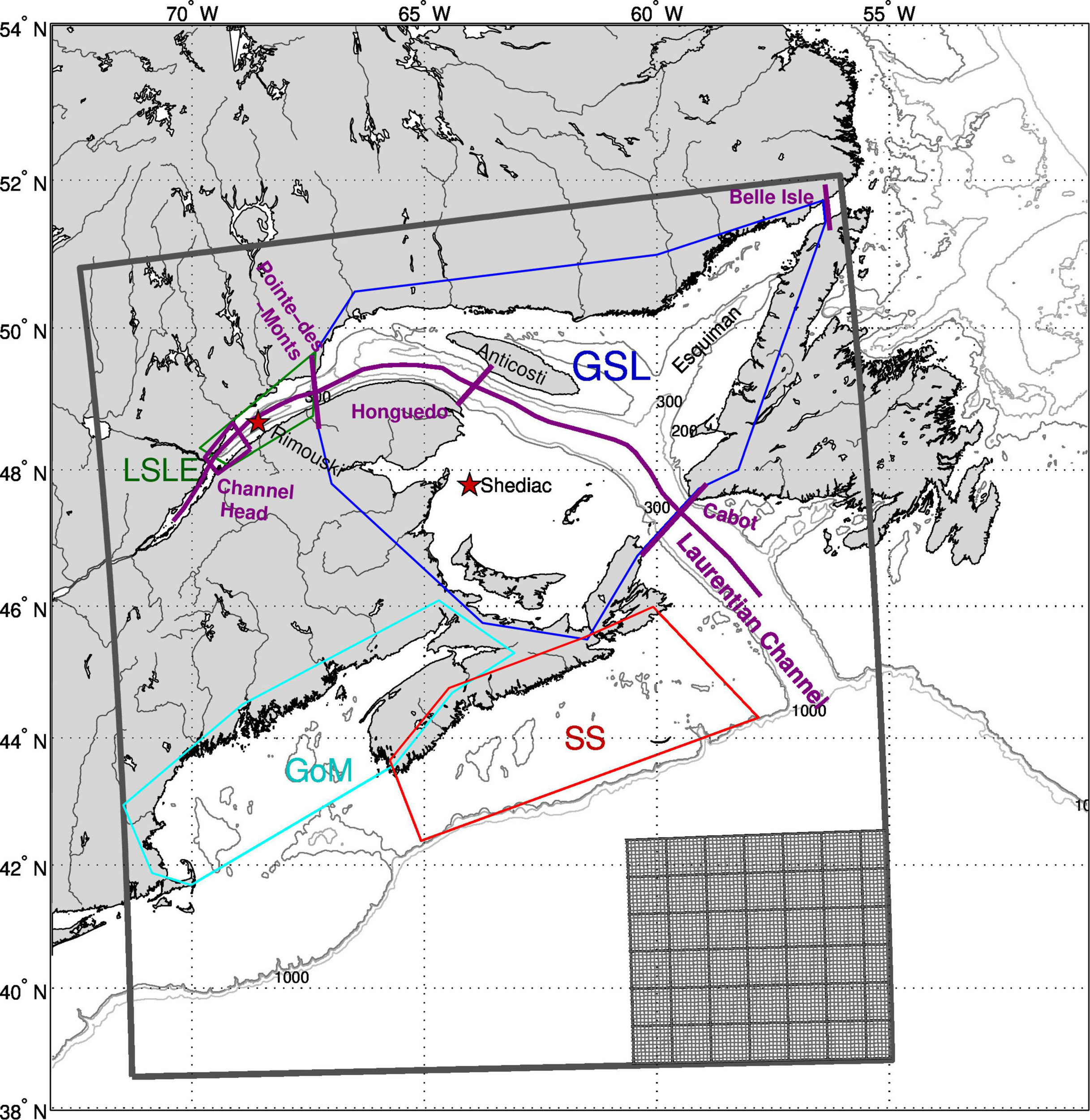
Figure 1. Map of the study area showing the model domain, with a small sub-area showing the grid size in the lower right corner. The 200, 300, and 1000 m depth contours are shown. The purple lines show the position of the transects used in some figures or for transport comparison (Pointe-des-Monts, Honguedo, Cabot Strait, and the Strait of Belle Isle). The line following the Laurentian Channel indicate the positions where data are presented in some figures. The purple box indicate the area over which vertical nitrate fluxes are calculated, while the larger boxes (LSLE in green, GSL in blue, SS in red, and GoM in cyan) represent the regions where average quantities are calculated in some figures. The stars indicate the location of two fixed AZMP stations (Rimouski and Shediac) from which data are used to validate the model.

The shallow southern GSL, represented in large part by the Magdalen Shallows, receives part of the nutrients carried by the relatively fresh surface waters, although the importance of this nutrient source for local primary production is uncertain (Sinclair et al., 1976; de Lafontaine et al., 1991; Levasseur et al., 1992; Cyr et al., 2015). The northeast GSL, on the other hand, is less subject to the direct influence of freshwater runoff. The northeast is less stratified than the other regions of the GSL and under the direct influence of water flowing in from the Labrador Shelf and Atlantic Ocean, which have lower nutrient concentrations compared to the LSLE (Starr et al., 2004). Differences in nutrient sources lead to heterogeneous conditions in primary production in the GSL (de Lafontaine et al., 1991 and references therein; Lavoie et al., 2008). The geographic location of the GSL, in combination with its complex topography and circulation, also lead to the aggregation of large quantities of krill (Simard and Lavoie, 1999; Maps et al., 2015; Lavoie et al., 2016) and copepods (Maps et al., 2011; Brennan et al., 2021) that are sought as food by endangered whales (blue whales (Lesage et al., 2018), North Atlantic right whales (Simard et al., 2019) that visit the GSL for many months each year.

The deep waters of the GSL also present particularly low concentrations of dissolved oxygen (DO), pH (∼7.5, total scale) and calcium carbonate saturation states (below unity for both aragonite and calcite), especially in the LSLE (Gilbert et al., 2005; Mucci et al., 2011; DFO, 2020). At depths below about 200 m, DO concentrations decrease from about 180 mmol m^–3 at Cabot Strait to 60 mmol m^–3 at the head of the Laurentian Channel (Gilbert et al., 2005). This decrease in DO is accompanied by an increase in DIC (Mucci et al., 2011). Nitrate and silicate concentrations, on the other hand, increase by about 2 mmol N m^–3 and 15 mmol Si m^–3 respectively (Coote and Yeats, 1979), as the water moves up towards the head of the Laurentian Channel. Two main factors are responsible for these gradients: (1) the proportion of Labrador Current and North Atlantic Central waters in the mixture that enters the Laurentian Channel, since these water masses have different chemical properties, and (2) the sinking and remineralization of organic matter produced in the surface layer by primary producers and supplied by the rivers (Gilbert et al., 2005; Claret et al., 2018; Lavoie et al., 2019). These processes lead to loss of oxygen and acidification in the deep water of the LSLE where ventilation is weak (Gilbert et al., 2005; Mucci et al., 2011). Low pH (<7.7, total scale) and calcium carbonate saturation states below unity (even for calcite over a few months in summer or fall) are also found in the shallower southern GSL (Menu-Courey et al., 2019; DFO, 2020).

Substantial interannual variability in physical, biological and chemical conditions is also present in the system. For example, the sea-ice cover in the GSL, whose demise controls the initiation of the phytoplankton bloom in many regions (Le Fouest et al., 2005), is highly variable from one year to the next; record high and low volumes were observed within a few years in the last decades (Galbraith et al., 2016). Large anomalies in river runoff and wind forcing, which affect circulation patterns and strength in the GSL (Saucier et al., 2009; Lavoie et al., 2016; Lavoie et al., 2017) have been observed locally (Galbraith et al., 2016), and in the northwest Atlantic (Hu et al., 2011; Peterson et al., 2017). These large interannual variations in forcing result in large primary and secondary production variability (Plourde et al., 2014), and have an impact on the properties of the water masses that enter the GSL.

The GSL is also impacted by climate variability and change. Long term trends in physical and chemical conditions have been recorded in the GSL, such as warming of surface and sub-surface waters (Galbraith et al., 2012; Loder et al., 2013), deoxygenation (Gilbert et al., 2005; Claret et al., 2018; Jutras et al., 2020), and acidification (Mucci et al., 2011) of the deep Laurentian Channel waters. These trends are similar to those obtained with Earth System Models near the mouth of the Laurentian Channel and are projected to continue in the future (Lavoie et al., 2019). These changes have an impact on the health and distribution of the various marine organisms that live in these waters (Bianucci et al., 2016; Brennan et al., 2016; Stortini et al., 2017; Greenan et al., 2019), of which many are of commercial importance. Commercial fisheries totaled $3.0 billion in the DFO’s Atlantic regions (Maritimes, Gulf, Quebec and Newfoundland and Labrador) in 2016 (Lobster Fishing Areas 27 - 38 - Integrated Fisheries Management Plan²). Within the GSL, American lobster and snow crab are the most important fisheries, especially in the southern Gulf, with shrimp and groundfish also being important in the deep channels of the northern GSL (DFO, 2011a, b; Gaudet and Leger, 2011). The GSL is also of great importance for Atlantic Salmon as it has many salmon rivers and salmon smolts spend a few months in the GSL in summer before migrating to the Labrador Sea (e.g., Ohashi and Sheng, 2018).

To better understand the functioning of the ecosystem and to project the evolution of primary production, deoxygenation and acidification within the GSL, the use of a high-resolution regional model is required.

Different NPZD (nutrient-phytoplankton-zooplankton-detritus) models have been implemented in the GSL. Zakardjian et al. (2000) implemented a 1D and a 2D model in the LSLE to test the importance of diatom sinking speed and horizontal advection on the observed delay of the phytoplankton spring bloom in that region. Tian et al. (2000) implemented a 1D model in the center of the nwGSL cyclonic gyre. They highlighted the importance of organic matter remineralization and nitrification taking place below the euphotic layer, but above the winter mixed layer depth, as a nutrient source to the surface layer, as well as the importance of the sinking of large particles for the export of carbon below the winter mixed layer. A slightly modified version of the latter model was also implemented in Bonne Bay, Newfoundland, to look at the processes leading to the relative constancy of export fluxes from spring to fall (Tian et al., 2001). Le Fouest et al. (2005), hereafter identified as LF05, then implemented a moderately complex NPZD model into a 3D ocean circulation model of the whole GSL in order to identify the physical forcing governing primary production in different regions of the GSL. Subsequent improvements were brought to the original model: light attenuation by colored dissolved organic matter (CDOM) as a function of surface salinity and phytoplankton photoadapation (Le Fouest et al., 2006, 2010). Mei et al. (2010) implemented CDOM explicitly, as a passive tracer, rather than as a function of salinity as in Le Fouest et al. (2006). They also added a temperature sensitive maximum growth rate for phytoplankton and zooplankton. Their goal was to look at the importance of these parameters to the timing of the phytoplankton bloom.

However, although the LF05 model reproduces some characteristics of the system, a drift of the biogeochemical conditions is present, limiting its use for multi-year simulations aimed at analysing interannual variability or climate change. In this paper, we describe GSBM (the Gulf of St. Lawrence Biogeochemical Model), which is based on LF05, but to which numerous improvements were made to better represent the microbial loop and maintain realistic biogeochemical conditions over the long term. The importance of properly representing and/or parameterizing the processes (sinking speed, fragmentation and remineralization rates) affecting particulate organic matter in numerical models to reproduce the biogeochemical tracers distribution in the marine environment has been reported many times (Fasham and Evans, 1995; Kawamiya et al., 1995, 1997; Haigh et al., 2001; Kriest et al., 2012; Kriest and Oschlies, 2015; Baker et al., 2017; Lavoie et al., 2019). GSBM also includes a DO module, a carbonate chemistry module, as well as the supply of organic and inorganic nutrients, DIC and alkalinity by rivers. GSBM is coupled to the ocean circulation model CANOPA. In the following sections, we describe the different components of the model and show its skill at reproducing the important biogeochemical features of the ecosystem.

Model Description

Ice-Ocean Model CANOPA

The ocean circulation model used in our study, described in detail in Brickman and Drozdowski (2012) and with additional validation in Lavoie et al. (2016), is based on the Nucleus for European Modelling of the Ocean (NEMO) system. The modelling system is based on the Océan PArallélisé code, version 9.0 (OPA; Madec, 2012). A thermodynamic-dynamic sea-ice model, Louvain-la-Neuve Sea Ice Model (LIM2; Madec et al., 1998), is coupled to the circulation model. The grid of the model covers the GSL, the Scotian Shelf, and the Gulf of Maine (GoM; Figure 1). The grid has a horizontal resolution of 1/12° in latitude and longitude (about 6 × 8 km depending on the location) and 46 layers of variable thickness (from 6 m close to the surface to 250 m at depth in the ocean).

It is a prognostic model, meaning that the temperature and salinity fields are free to evolve with time and are only constrained through open boundary conditions, freshwater runoff, and surface forcing. We use the Brickman and Drozdowski (2012) monthly climatologies of temperature and salinity to initialize the model and set the open boundary conditions. These were built from extensive Fisheries and Oceans Canada databases covering the 1971–2000 period. An annual cycle of the barotropic transport is prescribed at the Strait of Belle Isle in addition to a smaller baroclinic transport calculated from the monthly temperature and salinity fields. Tidal components (M2, S2, N2, O1, and K1) are included in the model through surface elevation and barotropic transport at the open boundaries.

Freshwater enters the domain through precipitation and runoff from the 78 main rivers. The monthly runoff of the St. Lawrence River is estimated from sea level measurements at Lauzon using the approach of Bourgault and Koutitonsky (1999) and obtained from the St. Lawrence Global Observatory³. Runoff for all other rivers is obtained from a hydrological model described in Lambert et al. (2013). The hydrological model provides natural runoff curves (i.e., following precipitation and evaporation). Some of the simulated seasonal runoff curves were modified to take into account the presence of large hydro-electric dams (Saguenay, Manicouagan, Betsiamites and Outardes rivers, see Lavoie et al., 2017). We use three-hourly surface forcing data (air temperature, relative humidity, winds, cloud cover, and precipitation) obtained from the Canadian Meteorological Centre - Global Environmental Multiscale (CMC-GEM) atmospheric model (Pellerin et al., 2003) to force the ice–ocean model.

Biogeochemical Model

GSBM simulates the biogeochemical cycles of dissolved oxygen, inorganic carbon and nitrogen, and the biological components that determine the dynamic of the planktonic ecosystem (Figure 2). The model has 11 state variables. It includes both simplified herbivorous and microbial food chains typical of bloom and post-bloom conditions. The export of biogenic matter to depth is mediated by the herbivorous food web (nitrate, large phytoplankton (diatoms), mesozooplankton, detrital particulate organic matter, while the microbial food web (ammonium, small phytoplankton, microzooplankton, dissolved organic matter) is mainly responsible for nutrient recycling in the euphotic zone. Nitrate (NO₃^–), ammonium (NH₄), dissolved organic nitrogen (DON), detrital particulate organic nitrogen (PON), DIC and total alkalinity (TA) are supplied by rivers. The tight coupling between small phytoplankton growth and microzooplankton grazing, microzooplankton egestion and detritus decay, DON remineralization to NH₄, and nitrification represent the dynamic of the microbial food chain. Biological variables are calculated in nitrogen units and algal biomass and production converted to chlorophyll a (chl a) and carbon units using fixed ratios. Detrital particulate organic matter sinks toward the bottom with a speed that varies regionally as a function of surface salinity to account for the influence of riverine input on organic matter aggregation and sinking. Sinking particles are gradually degraded into DON via a temperature-dependant fragmentation rate. The phytoplankton growth rate is a function of light and nutrient availability. The available light for phytoplankton growth is a function of sea-ice cover, chl a and turbidity (Le Fouest et al., 2006).

FIGURE 2

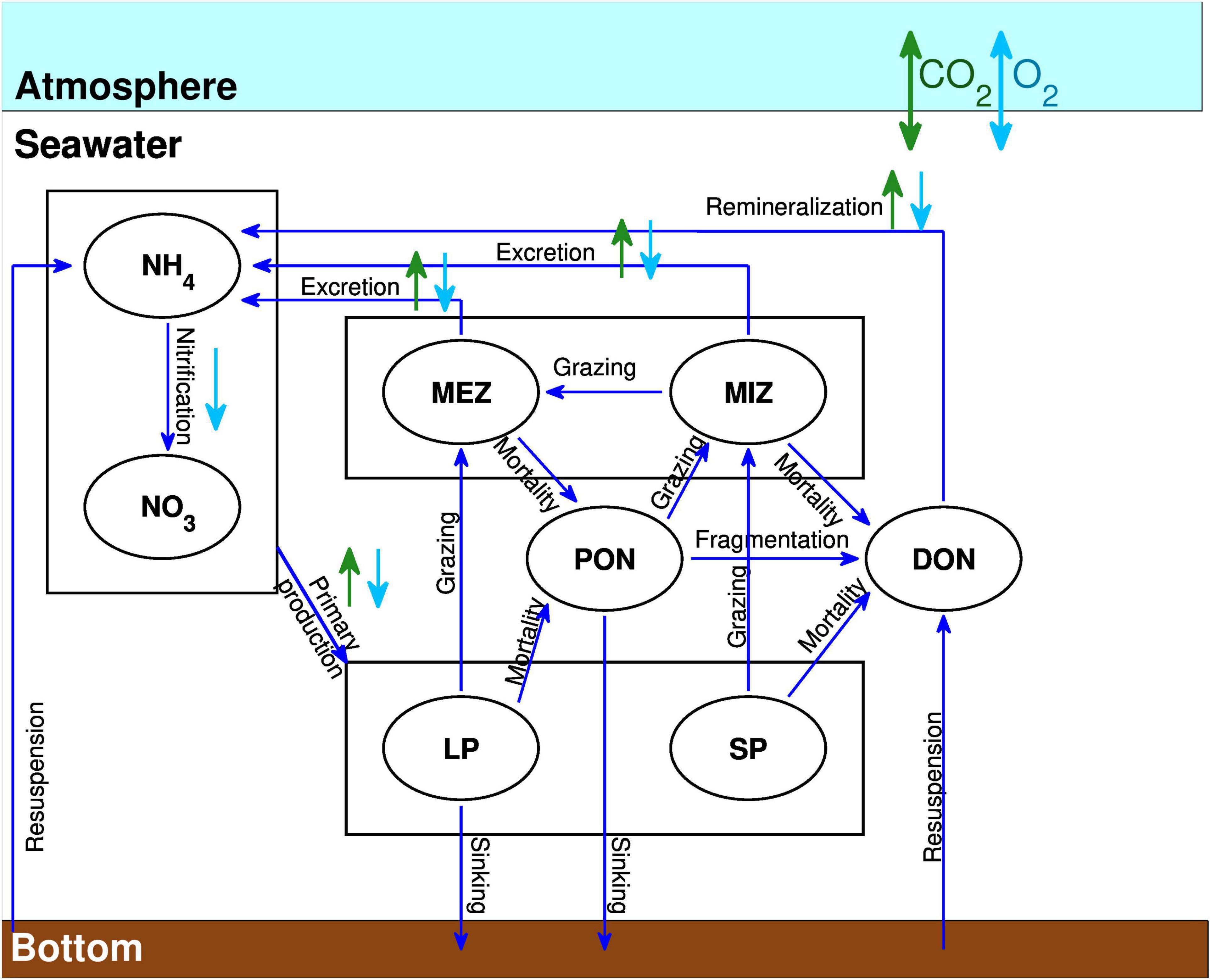
Figure 2. Conceptual planktonic ecosystem model including nitrate (NO3), ammonium (NH4), large phytoplankton (LP), small phytoplankton (SP), mesozooplankton (MEZ), microzooplankton (MIZ), particulate organic nitrogen (PON), and dissolved organic nitrogen (DON). Dark blue arrows represent nitrogen fluxes between the biological components, while the light blue and green arrows denote if the represented process lead to consumption (pointed downward) or production (pointed upward) of oxygen and CO₂, respectively.

Biological processes have an impact on the concentration of chemical constituents in the water column. DO and DIC production and consumption rates, as well as changes in TA are related to nitrogen transformations using constant ratios. Calcium carbonate saturations and pH are calculated using the carbonic acid dissociation constants of Lueker et al. (2000) and pH in the total scale (Dickson et al., 2007). Phosphate and silicate concentrations are not included in the calculations. The impact of omitting these nutrients in the calculation was evaluated to be smaller than 1% for calcium carbonate saturations in Barrow and Davies Straits (Azetsu-Scott et al., 2010). The main changes made to the original version of LF05 are summarized in Appendix A. A sensitivity analysis is also presented in the Supplementary Material for some of these changes (see Supplementary Figures 1–6). The equations of the model are detailed in section “Biogeochemical Model Equations”, while a list of parameters is given in Table 1.

TABLE 1

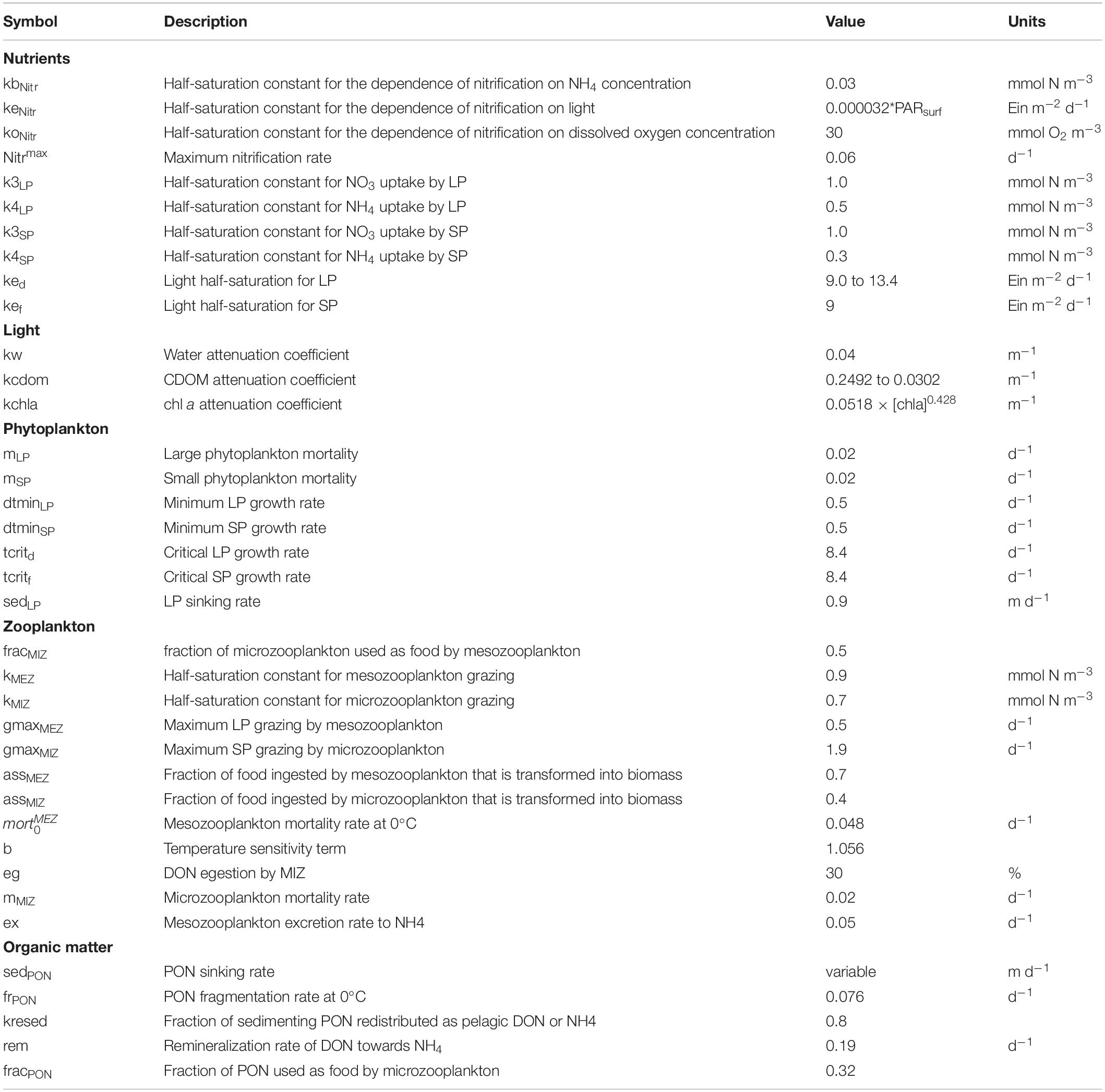
Table 1. Biogeochemical model parameters.

Data Used for Initial and Boundary Conditions, and Validation

Monthly climatologies of nitrate, DO, DIC and TA are used to initialise the model and provide lateral boundary conditions. Monthly climatologies of nitrate, DIC, and TA are also used for river input, except for the St. Lawrence River near Quebec City were DIC and TA are annual means.

Rivers

Nitrate

Nitrate concentrations in rivers were obtained from the different provincial departments (Ministère de l’Environnement et de la Lutte Contre les Changements Climatiques (MELCC) in Quebec, Water Quality and Quantity Section in New Brunswick, Department of Environment and Conservation in Newfoundland and Labrador) and from Environment Canada’s Atlantic Water Quality Monitoring program for Nova Scotia. Data were also obtained from Environment Canada’s database for different regions. Nitrate concentrations for the rivers located in the United States were obtained from the United States Geological Survey (National Water-Quality Assessment Program). Finally, data were extracted from the literature for some of the GSL’s north shore rivers (Walsh and Vigneault, 1986). The data were provided in mg N L^–1 and converted to mmol N m^–3 using a factor of 71.3944 (1000/14.0067).

The frequency of sampling varied among rivers. Sampling was defined as excellent when the 12 months of the year were sampled during at least six years (Figure 3). The data were qualified as good when 8 to 11 months were sampled for at least six years. Below this sampling frequency, the data were qualified as poor. Those rivers represented in the model for which no data are available are represented as No data in Figure 3A. A climatology of monthly nitrate concentration was prepared for the rivers qualified as good or excellent (Figure 3B). For the rivers where data are insufficient or lacking, we first defined regions with similar characteristics (in term of nitrate concentration, physiogeography and land use), and used the mean nitrate climatology of the region to fill in the gaps. The contours of the six regions are presented in Figure 3A.

FIGURE 3

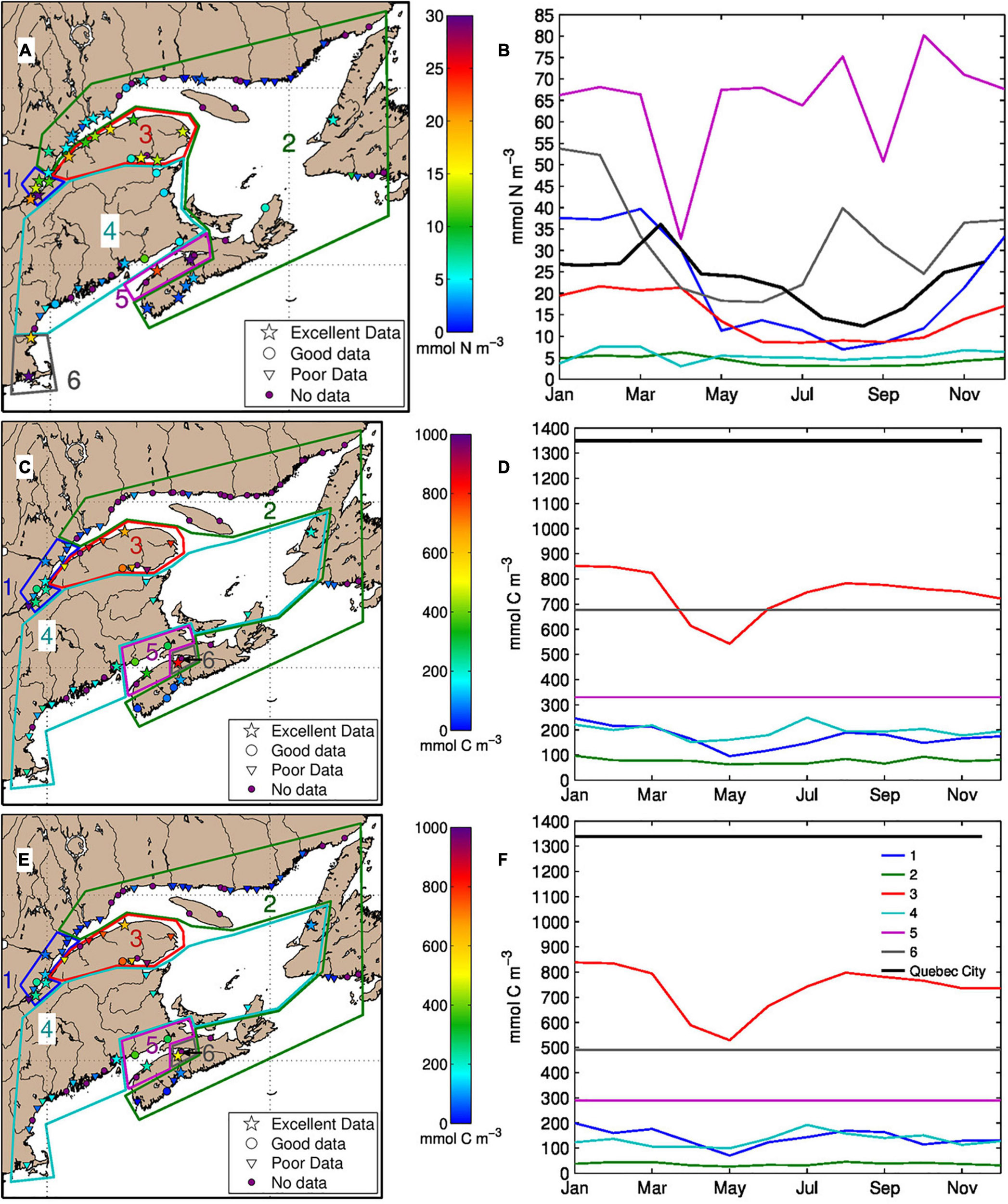
Figure 3. Contours of the six regions with rivers having similar characteristics for nitrate (A), dissolved inorganic carbon (C), and total alkalinity (E). The annual mean concentration are given for each rivers (colorbar) when data are available. The shape of the symbols indicates the quality of sampling in terms of frequency or when no data are available (purple circle). The panels to the right show the corresponding monthly climatology for each region and for Quebec City, or the constant annual mean when a climatology could not be calculated (B,D,F). The regions are different for nitrate than for dissolved inorganic carbon and total alkalinity.

The rivers flowing into the upper St. Lawrence estuary (region #1) display high nitrate concentrations due to the presence of numerous cities and farms in that area. The GSL’s north shore rivers, east of the Saguenay Fjord, as well as the Newfoundland and southern Nova Scotia rivers display the lowest nitrate concentrations (region #2). The northern Nova Scotia (region #5) and Massachusetts rivers (region #6), on the other hand, display the highest nitrate concentrations due to farming activities and large human populations.

Dissolved Inorganic Carbon and Total Alkalinity

The same approach and sources of data described above were used for river DIC and TA, although much less data were available for DIC than for nitrate (Figures 3C–F). However, pH and TA are more often sampled and we used the carbon equilibrium equations mentioned in section “Biogeochemical Model” to derive DIC concentrations. We use an annual mean value of 1350 mmol C m^–3 for DIC in the St. Lawrence River near Quebec City, as well as pH values provided by the MELCC to derive an annual mean TA of 1339 mmol C m^–3. These values are slightly higher than those reported in Dinauer and Mucci (2017) for DIC and TA at the same location (1242 mmol C m^–3 and 1205 mmol C m^–3 respectively).

The regions drawn for the estimation of the DIC and TA climatologies are slightly different than for nitrate (Figures 3C,E). Rivers in regions #1, #2, #4 and #5 present very low DIC and TA concentrations (as low as 50 mmol C m^–3 for DIC) while concentrations in rivers from regions #3 and #6 can reach 1000 mmol C m^–3 for DIC.

The DIC data were provided in mg C L^–1 and converted to mmol C m^–3 using a factor of 83.26 (1000/12.0107). The TA data were provided in mg CaCO₃ L^–1 and converted to mmol C m^–3 using a factor of 9.9913 (1000/100.0869).

Other Variables

Dissolved oxygen concentrations in rivers are calculated from the solubility equation (Benson and Krause, 1984), with river temperature set to the temperature of the nearest ocean grid cell of the model and salinity set to zero. Values for NH₄, and PON were set to 1.0 and 0.05 mmol N m^–3 respectively. DON was set to 3.0 mmol N m^–3 in most rivers. These are conservative estimates as the concentrations of these constituents are higher in the rivers flowing in the upper St. Lawrence Estuary (e.g., Hudon et al., 2017) and in other areas with important anthropogenic activities. We kept values in the lower range found for the GSL’s north shore river. DON measurements were made at a higher frequency in 8 rivers (St. Lawrence, Manicouagan, aux Outardes, Betsiamites, Mitis, Saguenay, Ouelle and Du Gouffre, Michel Lebeuf, Maurice Lamontagne Institute, personal communication, 2019) and were used to calculate annual mean values that are supplied to the model. These annual mean vary between about 6 mmol N m^–3 for 6 of the rivers, 15.8 mmol N m^–3 for the Ouelle river, and 19.1 mmol N m^–3 for the St. Lawrence River.

Initial and Open Boundary Conditions

An essential element to properly simulate the biogeochemical conditions of the system is to obtain realistic initial and open boundaries conditions, especially for the water masses that flow into the domain (e.g., water properties along the shelf edge south of Newfoundland, and deep water mass of the Laurentian Channel). We gathered as much data as possible over the model domain and just outside for nitrate, DO, DIC and TA to build monthly climatologies. The data were then interpolated over the entire model grid with an optimal linear interpolation technique using the OAX5 program developed at the Bedford Institute of Oceanography, Fisheries and Oceans Canada⁴. The spatial and temporal parameters for the interpolation varied from one variable to the other as a function of data coverage (large for nitrate, average for DO and weak for DIC and TA).

Nitrate

We use nitrate data gathered for the atlas of Brickman and Petrie (2003), that covers the GSL and the Scotian Shelf, data collected during the JGOFS program in the GSL (Roy et al., 2000), and data collected during the COUPPB program (Devine et al., 1997) and by Therriault and Levasseur (1985) in the St. Lawrence Estuary. Additional data were obtained from the BioCHEM database (Devine et al., 2014), and the World Ocean Database (Garcia et al., 2010b). We used the period 1981 to 2010 to build the nitrate climatology.

Dissolved Oxygen

The DO measurements were obtained from the BioCHEM database (Devine et al., 2014), and from the World Ocean Database up to 2006 (Garcia et al., 2010a). The DO concentrations obtained from the World Ocean Database were converted from ml L^–1 to mmol m^–3 using a factor of 44.6596 (García and Gordon, 1992). As for nitrate, we used data covering the 1981 to 2010 period to build the climatology.

Dissolved Inorganic Carbon and Total Alkalinity

The DIC and TA concentrations used for the interpolation of the initial and boundary conditions were obtained from GLODAPv2 (Key et al., 2015; Olsen et al., 2016), BioCHEM (Devine et al., 2014), and from the St. Lawrence Global Observatory (see text footnote 3) for some older data in the LSLE. As for rivers, TA and pH are usually the variables that are measured and we used the carbon equilibrium equations mentioned in section “Biogeochemical Model” to derive DIC concentrations. Since there are fewer observations available compared to nitrate and DO, we kept all the available data to build the monthly climatology (1980 to 2016).

Biogeochemical Model Equations

The model equations for the NPZD model are based on LF05. The choice of the NPZD model parameters is discussed in detail in LF05 and will not be repeated here. Testing of the LF05 parameters and results were also performed in subsequent studies in the GSL (Le Fouest et al., 2006, 2010; Lavoie et al., 2008; Mei et al., 2010) and in Hudson Bay (Sibert et al., 2011). The addition of a DO module was also tested by Nicot (2013) and Lavoie et al. (2015). However, since changes were made to these components (NPZD and DO) and that a carbonate system module was added, we detail all the equations below. The resulting model was tested over many years, one parameter at a time, to understand the functioning of this complex ecosystem, and whose large domain encompasses freshwater to oceanic conditions. The parameter values that were retained are found in Table 1, while the parameters tested and their ranges found in the literature are presented in Supplementary Table 1.

Phytoplankton

Large Phytoplankton

The rate of change of the large phytoplankton (LP) biomass is equal to

$$\frac{dLP}{dt}=\left({\mathrm{\mu }}_{LP}-m_{LP}\right)LP-g{z}_{MEZ}\cdot fra{c}_{LP}\cdot MEZ-se{d}_{LP}\frac{\mathrm{\delta }LP}{\mathrm{\delta }z},(1)$$

where μ_LP is the large phytoplankton specific growth rate, m_LP is the large phytoplankton mortality rate, gz_MEZ is the mesozooplankton grazing rate (see section “Small phytoplankton”), frac_LP is the fraction of the mesozooplankton diet composed of LP, MEZ is the mesozooplankton biomass, and sed_LP is the large phytoplankton sinking rate. The phytoplankton growth rate is formulated as in LF05 and is a function of both light and nitrogen availability. However, we modified the formulation of the light-based (dtc) doubling time by using a variable light half-saturation (ke_d) for LP to account for spatial differences in photoacclimatation (e.g., Le Fouest et al., 2010).

$${\mathrm{\mu }}_{LP}=\frac{\ln \left(2\right)}{\max (dt{n}_{LP},dtc)}(2)$$

with

$$dtc=dt\min {}_{LP}(1+\frac{k{e}_d}{PAR})(3)$$

and

$$dt{n}_{LP}=\frac{dt{\min }_{LP}}{f{\left(N\right)}_{LP}}(4)$$

where dtmin_LP is the minimum doubling time of the biomass, and PAR is the photosynthetically available radiation experienced by phytoplankton. The light half-saturation, ke_d, is equal to −26kcdom+16, where kcdom varies with surface salinity (between 0.2492 for salinities smaller than 26 and 0.0302 for salinities higher than 32) following Le Fouest et al. (2006).

We use the formulation proposed by Vallina and Le Quéré (2008) for the uptake of dissolved inorganic nitrogen by phytoplankton to avoid the inhibition of ammonium uptake by nitrate, which is present with the O’Neill parameterization used by LF05. For large phytoplankton

$$f{\left(N\right)}_{LP}=NuNH{4}_{LP}+NuNO{3}_{LP}(5)$$

$$NuNH{4}_{LP}=\frac{N{H}_4}{k{4}_{LP}+N{H}_4}(6)$$

$$NuNO{3}_{LP}={\displaystyle \frac{N{O}_3\left(1-NuNH{4}_{LP}\right)}{k{3}_{LP}+N{O}_3}}(7)$$

where NuNO3_LP and NuNH4_LP are the nitrate and ammonium uptake fractions respectively. Values for the half saturation constants for ammonium (k4_LP) and nitrate (k3_LP), as well as large phytoplankton mortality (m_LP) and sinking (sed_LP) rates, are found in Table 1. The fraction of the mesozooplankton food composed of large phytoplankton is equal to

$$fra{c}_{LP}=\frac{LP}{foo{d}_{MEZ}}.(8)$$

Mesozooplankton food (food_MEZ) is described in section “Small phytoplankton.”

Small Phytoplankton

The rate of change of small phytoplankton (SP) biomass is equal to

$$\frac{dSP}{dt}=\left({\mathrm{\mu }}_{SP}-m_{SP}\right)SP-g{z}_{MIZ}\cdot fra{c}_{SP}\cdot MIZ,(9)$$

where μ_SP is the small phytoplankton specific growth rate, m_SP is the small phytoplankton mortality rate, gz_MIZ is the microzooplankton grazing rate (equation 16), frac_SP is the fraction of SP used as food by microzooplankton, and MIZ is the mesozooplankton biomass, The equations for small phytoplankton growth and nutrient uptake are similar to those described above for LP except for some of the parameters (see Table 1). The light half-saturation (ke_f) for SP is also constant (9 Ein m^–2 d^–1). SP is not sinking. The fraction of small phytoplankton that is grazed by microzooplankton is equal to

$$fra{c}_{SP}=\frac{SP}{foo{d}_{MIZ}}.(10)$$

Microzooplankton food (food_MIZ) is described in section “Microzooplankton.”

Zooplankton

Mesozooplankton

The rate of change of mesozooplankton biomass is equal to

$$\frac{dMEZ}{dt}=as{s}_{MEZ}\cdot g{z}_{MEZ}\cdot MEZ-m_{MEZ}\cdot MEZ-ex\cdot MEZ,(11)$$

where ass_MEZ is the mesozooplankton food assimilation efficiency (70%), gz_MEZ is the mesozooplankton grazing rate, m_MEZ the mesozooplankton mortality rate, and ex is the mesozooplankton ammonium excretion rate (0.05 d^–1).

The mesozooplankton grazing rate is formulated using a sigmoidal “Holling’s type III” functional response as in Lavoie et al. (2009).

$$g{z}_{MEZ}=g{max}_{MEZ}\left(\frac{foo{d}_{MEZ}^2}{foo{d}_{MEZ}^2+k_{MEZ}^2}\right),(12)$$

where gmax_MEZ is the maximum mesozooplankton grazing rate (0.5 d^–1), k_MEZ is the half-saturation constant for mesozooplankton grazing (0.9 mmol N m^–3), and food_MEZ is the mesozooplankton food. Mesozooplankton graze on both large phytoplankton and microzooplankton

$$foo{d}_{MEZ}=LP+fra{c}_{MIZ}\cdot MIZ,(13)$$

where frac_MIZ is the fraction of microzooplankton on which mesozooplankton graze (0.5).

The mesozooplankton mortality, m_MEZ, was modified to follow a temperature dependence as in Buitenhuis et al. (2006). This was necessary to improve the representation of the biogeochemical conditions in the western Scotian Shelf and GoM.

$$m_{MEZ}=mor{t}_{0{}^{\circ }C}^{MEZ}\cdot b^T,(14)$$

where $mor{t}_{0{}^{\circ }C}^{MEZ}$ is the mortality rate at T = 0°C (0.048 d^–1) and b (1.056) is the temperature dependence of mortality (b¹⁰ = 1.72).

Microzooplankton

The rate of change of microzooplankton (MIZ) biomass is equal to

$${\displaystyle \frac{dMIZ}{dt}}=as{s}_{MIZ}\cdot g{z}_{MIZ}\cdot MIZ-m_{MIZ}\cdot MIZ-g{z}_{MEZ}\left({\displaystyle \frac{MIZ}{foo{d}_{MEZ}}}\right)MEZ,(15)$$

where ass_MIZ is the fraction of food ingested by microzooplankton that becomes biomass (40%), gz_MIZ is the microzooplankton grazing rate, m_MIZ the microzooplankton mortality rate (0.02 d^–1), and the last term is the loss of microzooplankton to mesozooplankton grazing. The microzooplankton grazing is formulated with a sigmoidal “Holling type III” functional response as in LF05, but we added grazing on PON, in addition to grazing on small phytoplankton, and we modified some of the parameters.

$$g{z}_{MIZ}=g{max}_{MIZ}\left(\frac{foo{d}_{MIZ}^2}{foo{d}_{MIZ}^2+k_{MIZ}^2}\right),(16)$$

$$foo{d}_{MIZ}=SP+fra{c}_{PON}\cdot PON,(17)$$

where frac_PON is the fraction of PON on which microzooplankton graze (0.32) and k_MIZ is the half-saturation constant for microzooplankton grazing. The maximum microzooplankton grazing rate (gmax_MIZ) and half-saturation constant (k_MIZ) were slightly reduced compared to LF05 (to 1.9 d^–1 and 0.7 mmol N m^–3 respectively).

Detrital Particulate Organic Nitrogen

Particular attention has been paid to the fate of PON in this study. To reproduce the main biogeochemical characteristics of the system in both short and long term simulations, the remineralization of sinking PON needs to occur at the right depth. This was achieved by improving the parameterization of the sinking speed and remineralization rate, and by taking into account the influence of freshwater outflow on the sinking rate. The rate of change of PON is equal to

$${\displaystyle \frac{dPON}{dt}}=g{z}_{MEZ}\left(1-as{s}_{MEZ}\right)MEZ+m_{MEZ}\cdot MEZ+m_{LP}\cdot LP-g{z}_{MIZ}\cdot fra{c}_{PON}\cdot MIZ-f_g\cdot PON-se{d}_{PON}{\displaystyle \frac{\partial PON}{\partial z}},(18)$$

where fg is the fragmentation rate of sinking PON to DON. It is a function of water temperature (T) as in Aumont et al. (2015),

$$f_g=f{r}_{PON}\cdot b^T,(19)$$

where fr_PON is the fragmentation rate of PON at 0°C (0.076 d^–1) and b is the temperature sensitivity (1.056, b¹⁰ = 1.72). The last term of equation 18 represents the PON changes resulting from sinking in the water column. The sinking rate of PON (sed_PON) varies spatially as a function of surface salinity to account for the influence of river input on the size of PON aggregates (see Lucotte et al., 1991; Al Azhar et al., 2017),

$$se{d}_{PON}=\{\begin{array}{cc}\hfill 25m{d}^{-1}\hfill & \hfill 21>salinity\le 29\hfill \\ \hfill 16m{d}^{-1}\hfill & \hfill salinity\le 21or>29\hfill \end{array}(20)$$

These changes results in a greater amount of PON being remineralized in the water column compared to LF05.

Dissolved Organic Matter

Dissolved organic matter is supplied by rivers, and produced through microzooplankton excretion and mortality, small phytoplankton mortality, and through the fragmentation of PON. The rate of change of DON is equal to

$${\displaystyle \frac{dDON}{dt}}=g{z}_{MIZ}\cdot eg\left(1-as{s}_{MIZ}\right)MIZ+m_{MIZ}\cdot MIZ+m_{SP}\cdot SP+f_g\cdot PON-rem\cdot DON,(21)$$

where eg. (30%) is the fraction of unassimilated food grazed by microzooplankton that is egested as DON, and rem (0.19 d^–1) is the remineralization rate of DON towards ammonium by bacteria. A fraction of the PON and diatoms (kresed = 0.8) that is deposited to the sediments is returned instantaneously to the pelagic bottom layer (last grid cell in the water column) as ammonium (20%) and DON (80%). This remobilization was added to account for regeneration processes occurring in the sediment which are of importance in shallow areas such as the southern GSL and Scotian Shelf, and at the head of the deep channels.

$$\frac{dDON}{dt}\left(bottom\right)=0.8\cdot kresed\left(\frac{se{d}_{PON}\cdot PON+se{d}_{LP}\cdot LP}{\mathrm{\Delta }z\left(bottom\right)}\right),(22)$$

where Δz is the thickness of the pelagic bottom layer.

Nutrients

Nitrate

Besides the nitrate supply at the model boundaries (rivers and ocean), nitrate production occurs through the oxidation of ammonium, while losses occur through consumption by phytoplankton,

$${\displaystyle \frac{dNO3}{dt}}=-{\mathrm{\mu }}_{LP}\cdot NuNO{3}_{LP}\cdot LP-{\mathrm{\mu }}_{SP}\cdot NuNO{3}_{SP}\cdot SP+Nitr\cdot N{H}_4(23)$$

where μ_LP and NuNO3_LP are the diatom growth rate and NO₃ uptake fraction respectively, μ_SP and NuNO3_SP are the flagellate growth rate and NO₃ uptake fraction, and Nitr is the ammonium oxidation rate (nitrification). We implemented nitrification as in Sibert et al. (2011) except that we added two additional terms to take into account the reduced nitrification in the euphotic zone (resulting either from light inhibition or from competition between phytoplankton and nitrifying bacteria) and under low DO conditions (Ward, 2000), which are found in bottom waters of the GSL.

$$Nitr=Nit{r}^{\max }\mathrm{}\left(1-\frac{PAR\left(z\right)}{PAR\left(z\right)+k{e}_{Nitr}}\right)\mathrm{}\left(\frac{N{H}_4}{N{H}_4+k{b}_{Nitr}}\right)\mathrm{}\left(\frac{DO}{DO+k{o}_{Nitr}}\right),(24)$$

where Nitr^max is the maximum nitrification rate, PAR(z) is the light intensity in the middle of layer z, ke_Nitr, kb_Nitr, and ko_Nitr are the half-saturation constants for the dependence of nitrification on light and NH₄ and DO concentrations respectively (see Table 1).

Ammonium

Changes in ammonium concentration result from phytoplankton uptake, excretion by meso- and microzooplankton, remineralization of DON and nitrification.

$$\frac{dNH4}{dt}=\mathrm{}-{\mathrm{\mu }}_{LP}\cdot NuNH{4}_{LP}\cdot LP-{\mathrm{\mu }}_{SP}\cdot NuNH{4}_{SP}\cdot SP\mathrm{}+ex\cdot MEZ+g{z}_{MIZ}\left(1-eg\right)\left(1-as{s}_{MIZ}\right)MIZ\mathrm{}+rem\cdot DON-Nitr\cdot N{H}_4.(25)$$

A small fraction (16%, or 20% of the 80% being returned to the pelagic bottom layer) of the PON and diatoms settling on the bottom is also remineralized to NH₄,

$$\frac{dNH4}{dt}\left(bottom\right)=0.2\cdot kresed\left(\frac{se{d}_{PON}\cdot PON+se{d}_{LP}\cdot LP}{\mathrm{\Delta }z\left(bottom\right)}\right).(26)$$

Dissolved Oxygen

The DO model follows the approach of Jin et al. (2007) such as described in Nicot (2013). The main change here, compared to the implementation of Nicot (2013), is in the addition of DO consumption by nitrification. The pathways of oxygen production and consumption are depicted in Figure 2. The changes in DO result from the differences in biological production and consumption, as well as from air-sea fluxes in the surface layer. The changes resulting from biological processes are

$$\frac{dDO}{dt}=P\mathrm{\_}{O}_2-C\mathrm{\_}{O}_2,(27)$$

where the production rate of DO (P_O₂) is equal to the sum of new and regenerated production by large and small phytoplankton

$$P\mathrm{\_}{O}_2\mathrm{}=r_{NP}\left({\mathrm{\mu }}_{LP}\cdot NuNO{3}_{LP}\cdot LP+{\mathrm{\mu }}_{SP}\cdot NuNO{3}_{SP}\cdot SP\right)\mathrm{}+r_{RP}\left({\mathrm{\mu }}_{LP}\cdot NuNH{4}_{LP}\cdot LP+{\mathrm{\mu }}_{SP}\cdot NuNH{4}_{SP}\cdot SP\right),(28)$$

with different stochiometric O₂:N molar ratios for new (r_NP = 138:16) and regenerated production (r_RP = 106:16).

Dissolved oxygen is utilized during the conversion of organic nitrogen to ammonium, mainly via remineralization of DON but also through zooplankton metabolism (ammonium excretion by mesozooplankton and microzooplankton), and nitrification. The consumption rate is given by

$$C\mathrm{\_}{O}_2\mathrm{}=r_{RO}\cdot ex\cdot MEZ+r_{RO}\cdot g{z}_{MIZ}\left(1-eg\right)\left(1-as{s}_{MIZ}\right)MIZ\mathrm{}+r_{RO}\cdot rem\cdot DON+r_{Nit}\cdot Nitr\cdot N{H}_4(29)$$

where r_Nit, the O₂:N molar ratio during nitrification, is equal to 2:1 as in Jin et al. (2007). According to Kortzinger et al. (2001) and references therein, the respirative ratio O₂:C_org for the remineralization of organic matter would have a value of about 1.34, which results in an O₂:N (r_RO) of 8.88 using the redfield ratio for C:N. This is close to our O₂:N molar ratios for new production defined above (8.625). We thus use the latter ratio (8.625) for the remineralization of organic matter.

The air-sea oxygen flux (F_O2) is parameterized using the standard transfer-velocity formulation of Wanninkhof (1992) for steady winds, based on the difference between the DO concentration at the surface and the oxygen saturation concentration.

$$F_{O2}=k_w\left(\left[O_2^{sat}\right]-\left[O_2\right]\right),(30)$$

where k_w is the gas transfer velocity for oxygen

$$k_w=\left(1-f\right)0.31{\left(\frac{S{c}_{O2}}{Sc20}\right)}^{-\frac{1}{2}}{W}^2,(31)$$

where f is the fraction of the sea surface covered with sea ice, Sc_O2 is the Schmidt number for oxygen in seawater computed using the formula of Wanninkhof (1992), Sc20 is the Schmidt number in seawater at 20°C (589.39) and W is the wind speed at 10 m in m s^–1. The oxygen saturation, O₂^sat, is computed from the simulated surface temperature and salinity following the equations established by Benson and Krause (1984).

Dissolved Inorganic Carbon

The solution of the carbonate chemistry equations follows Signorini et al. (2001). The cycling of DIC is coupled to the ecosystem model through biological consumption (C_CO₂) and production (P_CO₂) rates in a similar fashion to DO, except that it is not affected by nitrification. As for DO, the different pathways are depicted in Figure 2, and the equations are given below,

$$\frac{dDIC}{dt}=P\mathrm{\_}C{O}_2-C\mathrm{\_}C{O}_2(32)$$

$$P\mathrm{\_}C{O}_2\mathrm{}=r_{RC}\cdot ex\cdot MEZ+r_{RC}\cdot g{z}_{MIZ}\left(1-eg\right)\left(1-as{s}_{MIZ}\right)MIZ\mathrm{}+r_{RC}\cdot rem\cdot DON(33)$$

$$C\mathrm{\_}C{O}_2\mathrm{}=r{C}_{NP}\left({\mathrm{\mu }}_{LP}\cdot NuNO{3}_{LP}\cdot LP+{\mathrm{\mu }}_{SP}\cdot NuNO{3}_{SP}\cdot SP\right)\mathrm{}+r{C}_{RP}\left({\mathrm{\mu }}_{LP}\cdot NuNH{4}_{LP}\cdot LP+{\mathrm{\mu }}_{SP}\cdot NuNH{4}_{SP}\cdot SP\right).(34)$$

The C:N molar ratios are the same for new and recycled production (rC_NP = rC_RP = 106:16) and we use the same ratio (r_RC = 6.625) for the remineralization of organic matter. The air-sea CO₂ flux (FCO₂) is regulated by the gradient of the partial pressure (ΔpCO₂) across the air-sea interface, the piston velocity (k_w), and the solubility of CO₂ in seawater (α, in mmol m^–3 μatm^–1) which is a function of seawater temperature and salinity (Weiss, 1974).

$$FC{O}_2=k_w\cdot \mathrm{\alpha }\cdot \mathrm{\Delta }pC{O}_2(35)$$

$$\mathrm{\Delta }pC{O}_2=pC{O}_2^w-pC{O}_2^{atm}(36)$$

The direction of the flux is determined by the gradient of the partial pressure, where a negative flux indicates CO₂ uptake by the ocean, and a positive flux outgassing. The atmospheric pCO₂ (pCO₂^atm) time series used to force the model is based on the least square fit equation of Signorini et al. (2001) but with two different parameter values (A₀ = 334.05 μatm instead of 292.23, and A₁ = 0.0004 μatm month^–1 instead of 0.134) to obtain an increasing linear trend from one year to the other. Their model is at a similar latitude (50°N) as the northern portion of our model domain. Atmospheric pCO₂ is assumed to be the same over the whole domain. The partial pressure of dissolved CO₂ in seawater is defined by the relationship

$$pC{O}_2^w=[C{O}_2]/\mathrm{\alpha },(37)$$

where [CO₂] is the concentration of carbon dioxide in solution. We calculate [CO₂] from DIC concentration, TA and the carbonic acid dissociation constants (K₁ and K₂) of Lueker et al. (2000). The detailed method for the calculation of [CO₂] is provided by Dickson et al. (2007).

The piston velocity (k_w) is calculated as in equation 31 for DO but using the coefficients for CO₂ instead of O₂ in the calculation of the Schmidt numbers (Wanninkhof, 1992).

Total Alkalinity

Total alkalinity is unaffected by air-sea exchange of CO₂, and changed only slightly by biological production and remineralization of organic carbon. The model includes biological sources and sinks of alkalinity associated with nitrogen cycle processes including phytoplankton uptake, remineralization of organic nitrogen, and nitrification. The stoichiometry of these reactions is given by Wolf-Gladrow et al. (2007). Production and dissolution of biogenic carbonate minerals are neglected as is sedimentary denitrification. In the GSL, water column sources and sinks of alkalinity are small relative to fluvial sources (Figure 3), so the main controls on its distribution are dispersion and dilution of river water.

$$\frac{dTA}{dt}\mathrm{}=\left({\mathrm{\mu }}_{LP}\cdot NuNO{3}_{LP}\cdot LP+{\mathrm{\mu }}_{SP}\cdot NuNO{3}_{SP}\cdot SP\right)\mathrm{}-\left({\mathrm{\mu }}_{LP}\cdot NuNH{4}_{LP}\cdot LP+{\mathrm{\mu }}_{SP}\cdot NuNH{4}_{SP}\cdot SP\right)\mathrm{}+ex\cdot MEZ+g{z}_{MIZ}\left(1-eg\right)\left(1-as{s}_{MIZ}\right)MIZ\mathrm{}+rem\cdot DON-2\cdot Nitr\cdot N{H}_4.(38)$$

General Model Solution Description and Skill Assessment

The simulation is initiated May 1st 2005 and runs until the end of 2018. It takes a few years for the oceanic conditions near the open boundaries of the model to propagate up to the head of the deep Laurentian Channel (Bugden, 1991; Gilbert, 2004). We thus compare the model results with observations starting in 2009. Lavoie et al. (2016) demonstrated the performance of the CANOPA model in reproducing the hydrographic conditions of the GSL. Here we make a similar analysis of the model performance for the biogeochemical conditions, i.e., nitrate, ammonium, DIC and DO concentrations, TA, pH, and calcium carbonate saturations (calcite and aragonite). We use data from the same databases that were used to build the model initial and boundary conditions but collected after 2010. We also use ammonium, pH, and calcium carbonate saturation states data obtained from the BioCHEM database and from Pierre Pepin (Northwest Atlantic Fisheries Center, Fisheries and Oceans Canada) to validate the model results. A point-to-point comparison (same time and approximate location) is done between the model output and the observations. We use a Taylor diagram (Jolliff et al., 2009) to visualise the model skill at reproducing the different variables (Figure 4).

FIGURE 4

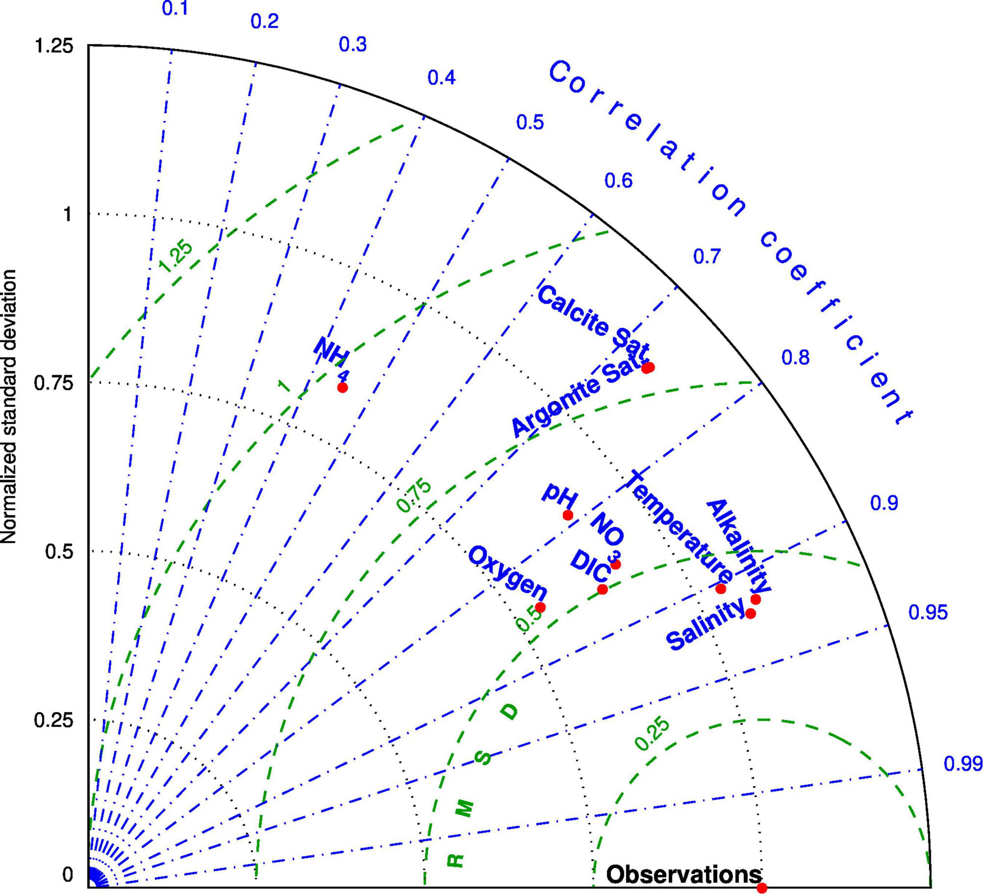
Figure 4. Taylor diagram of the model results for 2010 to 2017 over the whole domain. The blue dash-dot lines on the diagram represent the coefficient of correlation between the simulated and observed values. The green curved broken lines indicate the centered root mean square difference (RMSD) between the simulated and observed values. Finally the dotted lines show the normalized standard deviation of the simulated variables compared to the standard deviation of the observed field (value of 1.0). The closer the simulated values are to the point marked “Observations” on the x-axis the better the agreement.

Nitrate Concentrations

The spatial distribution of nitrate in the GSL has been mapped on the horizontal (Brickman and Petrie, 2003; Plourde et al., 2014) and on the vertical along the main channels (Coote and Yeats, 1979). The concentration of nitrate is sampled throughout the GSL twice a year, usually in June and late October, and in the surface layer in March, as part of the Atlantic Zone Monitoring Program (AZMP). The model reproduced well the observed horizontal and vertical distribution of nitrate reported in the above papers (correlation coefficient between simulated and observed values of about 0.85; Figure 4), with increasing concentrations towards the deeper layers and from the mouth of the Laurentian Channel towards its heads at depth (Figures 5A, 6A,E). The model also reproduced well the upwelling of nitrate-rich water at the head of the Laurentian Channel, the so called nutrient pump reported by Steven (1974). The average simulated nitrate flux for year 2010 across the 46-m horizon over the area depicted on Figure 1 at the head of the Laurentian Channel (magenta box) is equal to 18 mmol N m^–2 d^–1. Cyr et al. (2015) calculated fluxes between 18 and 300 mmol N m^–2 d^–1 in the area of maximal upwelling, that correspond to the western end of the box depicted in Figure 1. These nutrient-rich waters are mixed with the nutrient-rich fluvial input that lead to high nitrate concentration in the surface layer. The build up of nitrate in the surface layer and its downstream transport is particularly apparent in winter when nutrient uptake in the mixed layer is reduced and nitrate concentrations in rivers are high (Figures 3A, 5A). A minimum concentration is found in the subsurface layer of the LSLE. This feature is present in both the observations (Greisman and Ingram, 1977) and the model (Figure 6A).

FIGURE 5

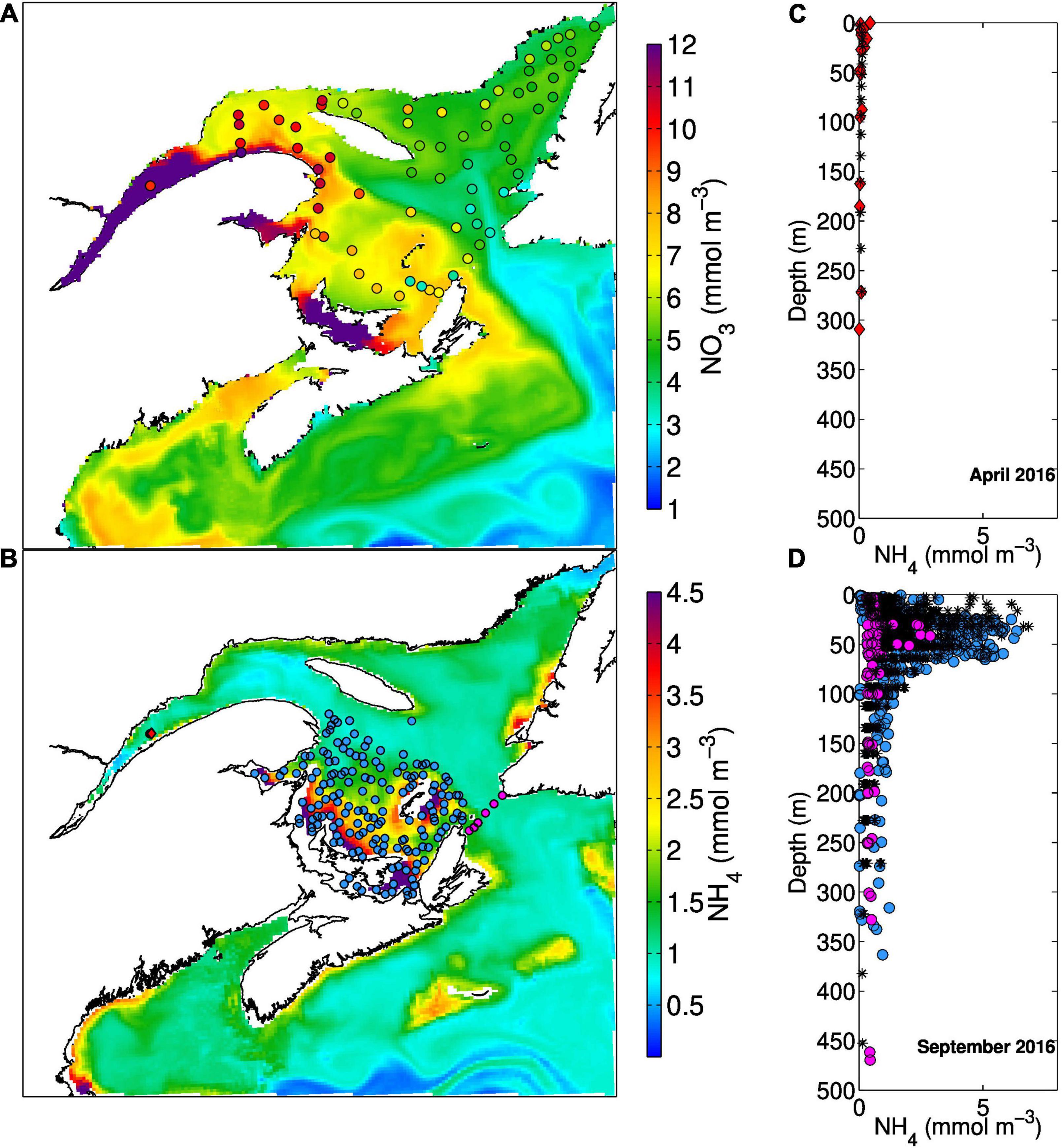
Figure 5. (A) Monthly mean simulated (background) and observed (dots) nitrate concentration in the surface layer (0-6 m for the model and 2 m for the observations) in March 2016. (B) Mean September 2016 ammonium concentration simulated by the model in the 28-58 m layer with position of samples taken in April at the Rimouski station (red diamond) and over the Magdalen Shallows (blue dots) and Cabot Strait (pink dots) in September. The vertical profiles corresponding to these locations are shown to the left (C,D) with the simulated values (corresponding in space and time to the measured profiles) represented by the black stars.

FIGURE 6

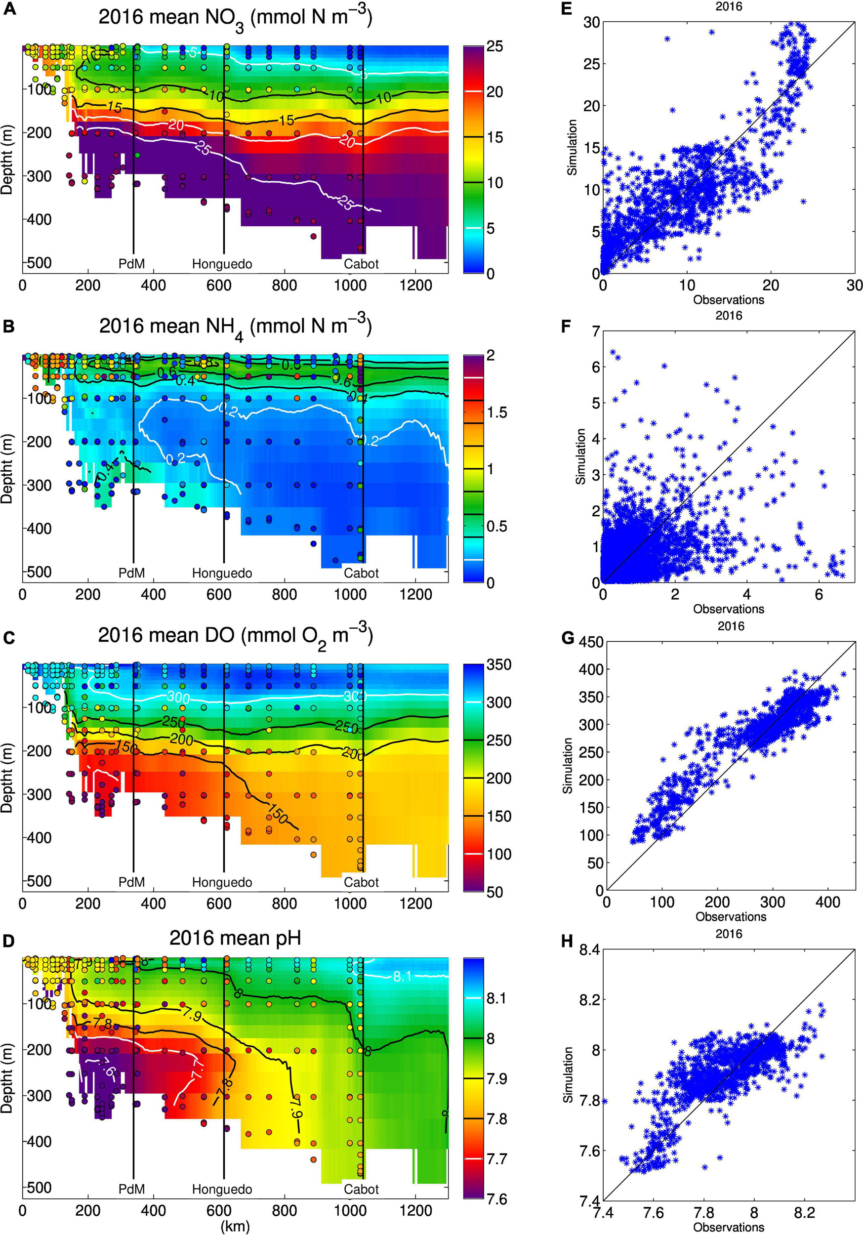
Figure 6. Simulated annual means (background colors) along the Laurentian Channel transect (see Figure 1) for (A) nitrate (mmol N m^–3), (B) ammonium (mmol N m^–3), (C) dissolved oxygen (mmol O₂ m^–3), and (D) pH_T in situ over the year 2016. The dots on top of the plot are observations made within 1 km of the Laurentian Channel transect (Figure 1) in the same year (punctual values are thus compared to the annual mean). The right panels (E–H) show a point by point comparison, in time and space, with available data over the whole domain.

Sinclair et al. (1976) and Cyr et al. (2015), contrary to Steven (1974), suggested that the LSLE nutrient pump was playing a minor role in primary production outside the LSLE. However, Sévigny et al. (1979) report that the estimate of Sinclair et al. for the seaward transport of nitrate in the upper layer of the LSLE needs to be corrected upward by a factor of 14 (this would result in a transport varying between 54.6 and 462 mol N s^–1 depending on the month) and that the nutrient pump would contribute to primary production in the Gaspé Current. Savenkoff et al. (2001), using inverse modelling, estimated the mean summer seaward nitrate transport from the LSLE in the 0-30 m layer at 460 mol N s^–1, which is similar to the highest (corrected) value of Sinclair et al. (1976). This value corresponds approximately to the mean simulated nitrate transport calculated in the upper 46 m at Pointe-des-Monts between May and September of 2009 to 2016 (472 mol N s^–1). The simulation shows that May to September is the period of the year when nitrate transport out of the LSLE in the upper layer is minimal (Pointe-des-Monts transect), while in fall and winter, transport over 1500 mol N s^–1 can be reached during particularly strong wind forcing events.

Large nitrate transport out of the GSL was also estimated at Cabot Strait in winter. Petrie and Yeats (2000) report that the GSL is the primary source of nitrate for the Scotian Shelf in winter (9300 mol N s^–1). The simulated nitrate fluxes towards the Scotian Shelf, at the same location and depth as in Petrie and Yeats (2000) are remarkably close to those estimated by the latter in both winter and summer months (Figure 7E). Overall, the nitrate distribution and transport calculated by the model at various locations in the GSL are in good agreement with those estimated in the literature.

FIGURE 7

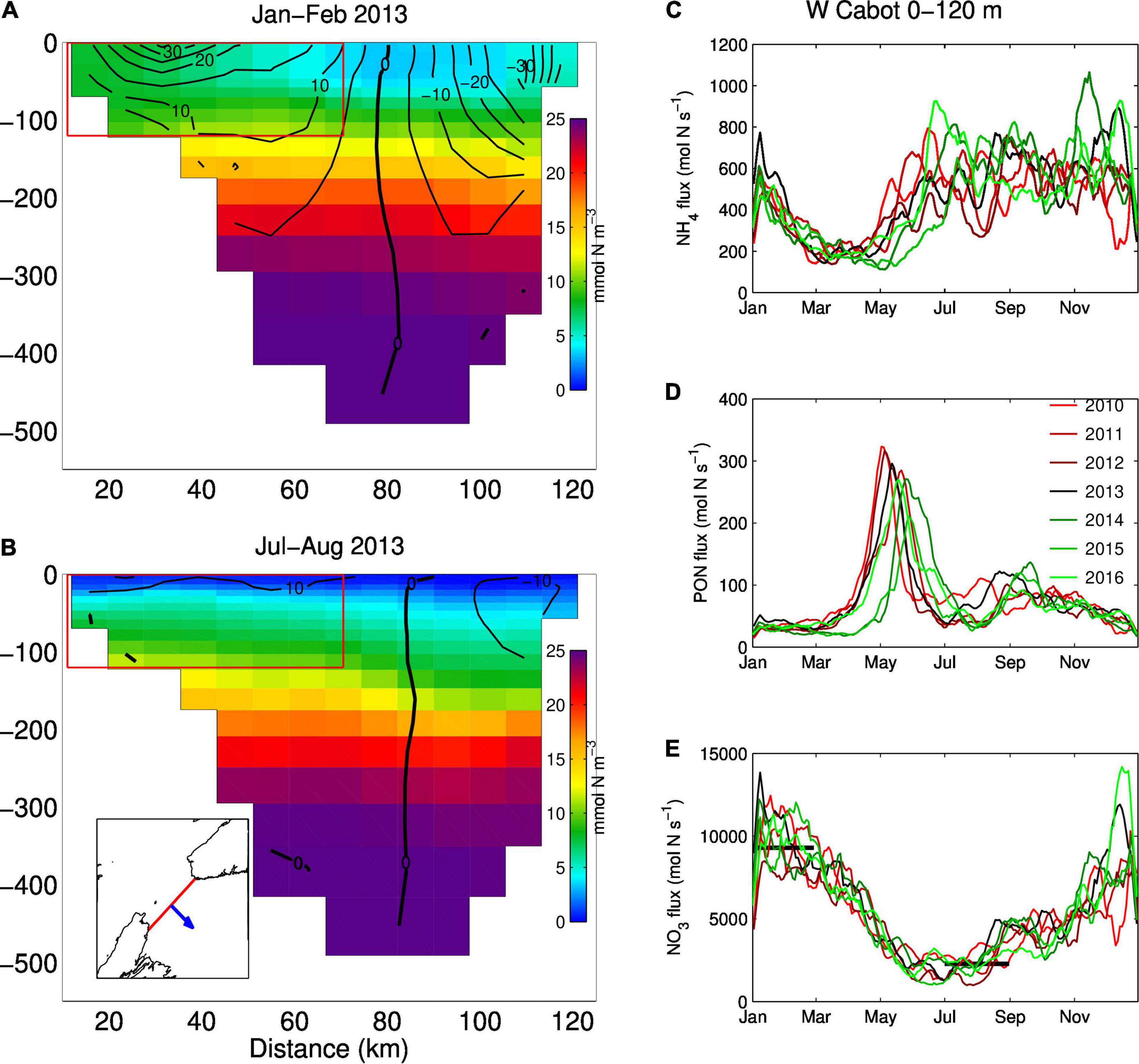
Figure 7. Mean nitrate concentrations (mmol N m^–3, background color) across the Cabot Strait section for (A) January and February, and (B) July and August 2013. The black lines represent the mean simulated velocities (cm s^–1) for the same months. The panels to the right show the mean transport through the western half of Cabot Strait (red box depicted in panels A and B) over the 0–120 m depth range for (C) ammonium (NH₄), (D) particulate organic nitrogen (PON) and (E) nitrate (NO₃^–). A positive value denotes an outflow. The black horizontal bars in panel E represent the mean nitrate transport estimated by Petrie and Yeats (2000) on the western side of Cabot Strait for depths of 0–150 m.

Ammonium Concentrations

Fewer data are available for ammonium concentrations compared to nitrate although they have been routinely collected as part of the AZMP in the last few years. Some measurements have also been reported in the literature for the LSLE (Therriault and Levasseur, 1985; Zakardjian et al., 2000) and GSL (Tremblay et al., 2000). The ammonium concentrations reported in these papers reached up to 4 mmol N m^–3 in the LSLE, at a depth of about 50m, while in the GSL, measured values reached 2.5 mmol N m^–3 at the base of the euphotic layer, with higher values during summer and on the Magdalen Shallows (up to 7 mmol N m^–3). The model results are consistent with high ammonium concentration on the Magdalen Shallows and at the base of the euphotic layer following primary production (Figures 5B,D, 6B,F). The model results indicate that part of the organic matter produced in the LSLE and in the nwGSL is transported towards the southern GSL where it is recycled and converted to ammonium and then nitrate. The addition of rapid remineralization of sedimenting PON in the bottom layer is particularly important in the reproduction of high ammonium concentration on the Magdalen Shallows. The recycling of sedimenting material in this shallow region, coupled to the strong stratification, explains the high nutrient concentrations found in the subsurface layer compared to concentrations found at similar depths in the adjacent Laurentian Channel (Coote and Yeats, 1979). It also leads to high simulated ammonium outflow at Cabot Strait (Figure 7C) in summer, even though the water transport is reduced at that time of the year (e.g., mean velocities in Figure 7B). The Taylor diagram (Figure 4) and the point to point comparison in Figure 6F indicate a low skill at reproducing the observed ammonium concentrations, even though we do reproduced its main features in the system (Figures 5B–D). The exact location of the base of the euphotic layer, were high ammonium values are found, might differ in the model. The timing for organic matter production and advection, and its recycling, can also be slightly different in the model. The analysis of ammonium concentrations was also done on frozen samples in many instances, which could lead to some contamination of the samples. There are thus many reasons that could explain the reduced correlation between observed and simulated ammonium concentrations.

Timing of the Phytoplankton Spring Bloom

We evaluate the capacity of the model to reproduce the phytoplankton spring bloom by comparing the simulated surface chl a with satellite-derived data averaged over specific areas (Figure 8). We also calculate the timing of the beginning of the spring bloom over each grid cell of the domain (Figure 8H) as the first day when chl a exceeds 1.45 mg m^–3. The map obtained with the simulated data is similar to other maps found in the literature (Siegel et al., 2002; Henson et al., 2009) and reproduces the known progression of the bloom, starting on the Scotian Shelf and then proceeding more or less counterclockwise around the GSL (de Lafontaine et al., 1991) following sea-ice retreat (Figures 8A,C). The main discrepancy occurs on the Magdalen Shallows, where the simulated bloom is delayed compared to the one estimated from the satellite data (Figure 8C). For the simulated estimate, the whole area of the box is taken into account, even the areas that are ice-covered (and thus present low chl a values). In the satellite data estimate, measurements are taken only in ice-free water but considered to represent the whole box. These differences could lead to a high bias in chl a concentrations estimated from satellite in early spring. Another discrepancy is noted in the nwGSL, where the fall bloom is not simulated.

FIGURE 8

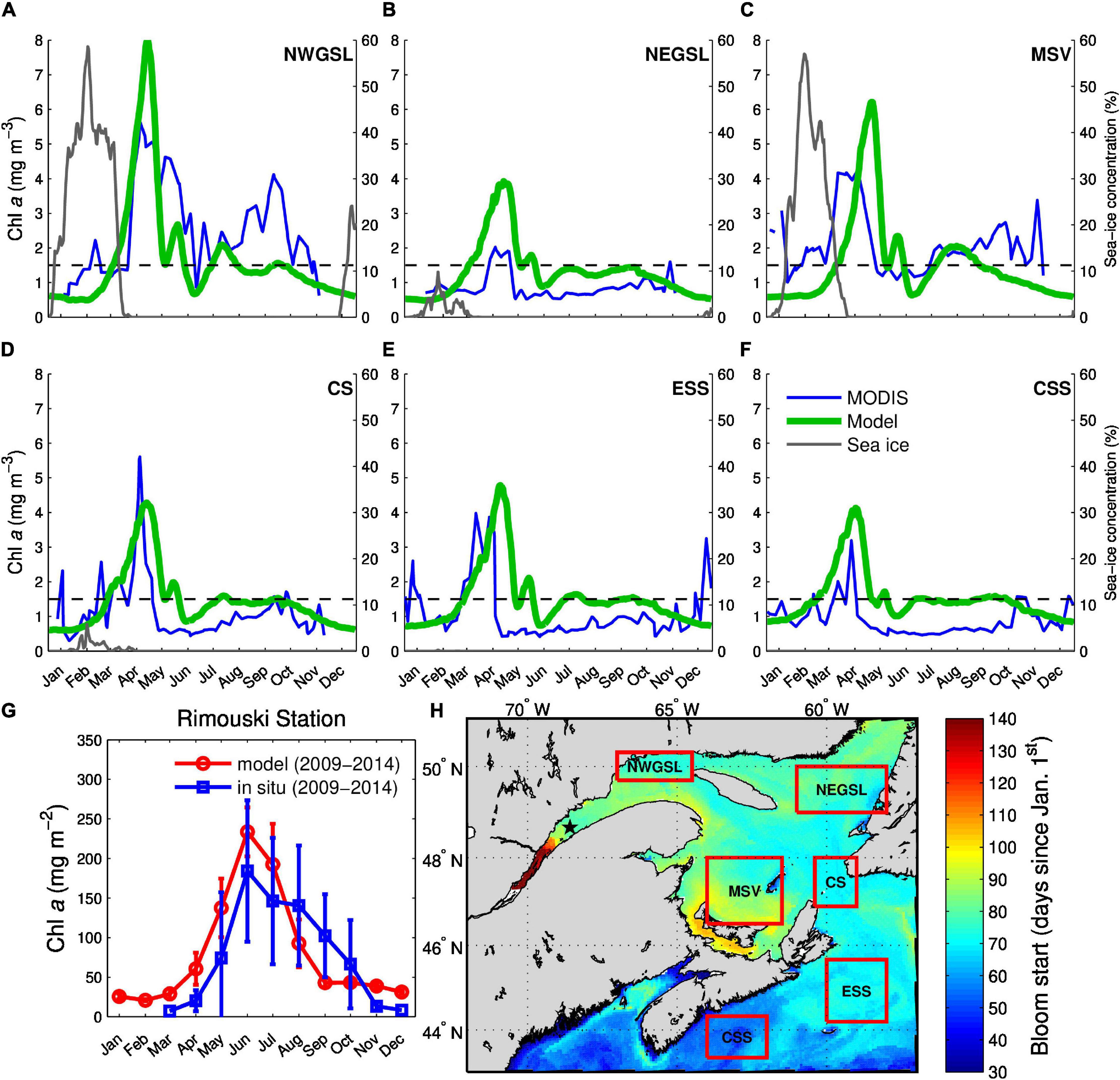
Figure 8. Mean surface chlorophyll a (mg chl a m^–3), simulated (green) and from satellite-derived data (MODIS, blue) over specific regions (panels A–F, see red boxes on the map in H) for the 2011 to 2013 period. The dotted line depicts the 1.45 mg chl a m^–3 threshold used to calculate the beginning of the bloom. The latter is shown in panel (H) (number of days from January 1st). The weekly mean chlorophyll a satellite data were obtained from the Bedford Institute of Ocean Sciences. Following Head and Pepin (2010), the mean values obtained with a box area coverage smaller than 10% were discarded. The gray line in panels (A–D) represent the average sea-ice concentration in the boxes. Panel (G) displays the 0–100 m integrated chl a (mg m^–2) at the AZMP Rimouski station in the Lower St. Lawrence Estuary (star on map in H) simulated (red) and measured in situ (blue) averaged over the 2009 to 2014 period.

In the LSLE, the phytoplankton bloom phenology is controlled in part by the turbidity of freshwater flowing into the estuary, which limits light availability, as well as by the strong horizontal advection, which in conjunction with the diatom sinking rate (larger sinking rates lead to a delayed bloom) can have a great impact on the timing of the bloom (Zakardjian et al., 2000). Satellite chlorophyll algorithms are not reliable in that area due to the large colored dissolved organic matter (CDOM) content of surface waters (Laliberte et al., 2018), and we use in situ data from the AZMP Rimouski station to evaluate the characteristics of the simulated phytoplankton bloom in that region (Figure 8G). The shape of the simulated chl a curve initially follows the in situ chl a curve, with a peak in June, as reported in the literature (end of June - early July, Levasseur et al., 1984; Therriault and Levasseur, 1985; Starr et al., 2004). However, the model does not capture the bloom characteristics from August to October with much smaller simulated values (falls outside of the observed standard deviation in October). The northeastern part of the LSLE, where inflow from the nwGSL occurs (Lavoie et al., 2016), presents characteristics that are more similar to those of the nwGSL with a bloom in April or May (Therriault and Levasseur, 1985; Roy et al., 2008; Xie et al., 2012).

Primary Production

Few measurements of primary production are available. Nevertheless, the model reproduced the known primary production spatial distribution (Figure 9), with higher primary production in the LSLE compared to the rest of the GSL (Steven, 1974; de Lafontaine et al., 1991; Fuentes-Yaco et al., 1997), as well as larger primary production on the Scotian Shelf and GoM compared to the GSL (Table 7 of Therriault and Levasseur, 1985). The mean primary production simulated by the model for years 2010 to 2016 falls within the values reported in the literature (Figure 9A). The main discrepancies between the simulated primary production and those reported in the literature occur in the Gaspé Current region, where simulated production is too low, and in the northeast GSL where it seems higher than observed [see Figure 6 of Lavoie et al. (2008)]. The simulated secondary production is high in the Gaspé Current region (Figure 9C), which most likely leads to the low primary production simulated by the model in this area.

FIGURE 9

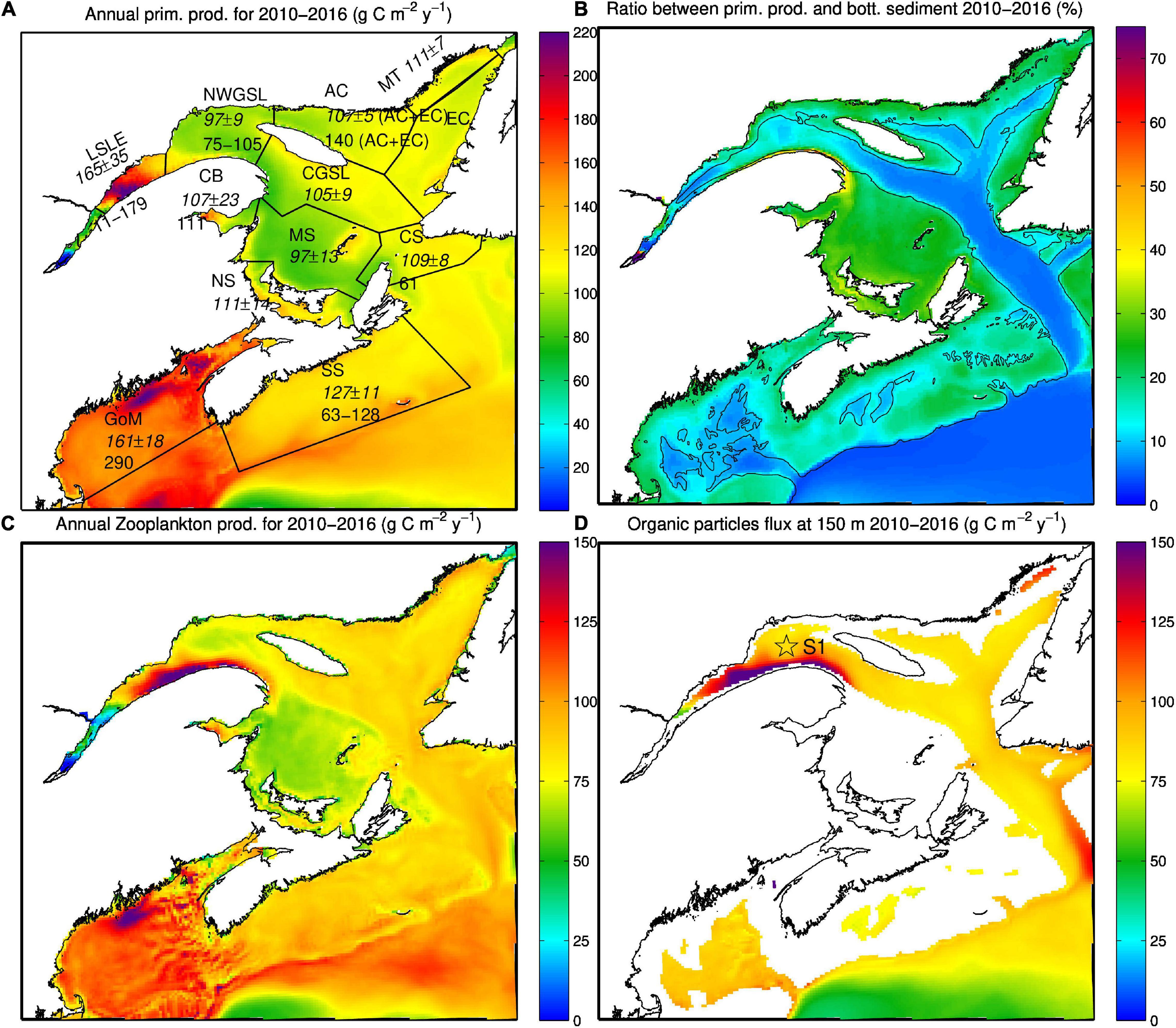
Figure 9. Averages, over the 2010-2016 period, of (A) primary production (background color, g C m^–2 y^–1), (B) percentage of primary production that reaches the sediments, (C) zooplankton production (g C m^–2 y^–1), and (D) particulate organic matter flux across the 150-m horizon. The average primary production calculated by the model as well as its standard deviation is displayed in italic in panel (A) for different regions (LSLE, NWGSL, AC, EC, CGSL, CB, MS, CS, SS, and GoM). The range of estimates from the literature is also displayed below the simulated average when available. The estimates are taken from Sinclair et al. (1976); Levasseur et al. (1984), and Therriault and Levasseur (1985) in LSLE, Sévigny et al. (1979) and Savenkoff et al. (1996) in the NWGSL, in Savenkoff et al. (1996) for AC+EC and CS, in Legendre (1971) for CB, in O’Reilly and Busch (1984) for the GoM, in Fournier et al. (1977); Mills and Fournier (1979), Mousseau et al. (1996), and Shadwick et al. (2011) for the SS. The 200 m isobaths is displayed in (B). Station S1 of Savenkoff et al. (1996) is displayed in panel (D).

Particulate Organic Matter

To successfully reproduce nutrient and DO concentrations as well as pH and calcium carbonate saturation states in the intermediate and deep layers, sinking and fragmentation rates of particulate organic matter must be represented correctly. The model results are very sensitive to these parameters (see Supplementary Figures 1, 2 in the Supplementary Material). Particulate and dissolved organic matter data are not available for a direct comparison but we can compare with concentrations and fluxes reported in the literature. Care must be taken when doing this comparison however, as only PON and DON of marine origin, as well as the labile fraction of riverine DON are considered in the model, while observations also include terrigeneous sources.

Lucotte et al. (1991) estimated that less than 30% of the primary production in the LSLE reaches the bottom sediment (mostly as fecal pellets), most of it (70%) being recycled in the water column. In the GSL, a lower percentage of the primary production would reach the sediment (7–10%; Savenkoff et al., 1996; Silverberg et al., 2000). These results are in line with a faster PON sinking speed in the LSLE (see section “Detrital Particulate Organic Nitrogen”). The model results are in accordance with these estimates, with 5 to 20% of the primary production reaching the sediments in the deep channels of the GSL (Figure 9B), the highest values being found in the downstream part of the LSLE. In shallower regions, this percentage is higher and reaches up to 50% around the Gaspé Peninsula (Figure 9B). This high percentage results in large part from the advection of phytoplankton and zooplankton in this region that leads to high PON sedimentation.

The particle flux calculated at 150 m in the model (Figure 9D) does not correspond as well with those reported by Savenkoff et al. (1996) at their station S1 (see Figure 9D), with estimated and simulated values of 45 ± 12 mg C m^–2 d^–1 and 80 mg C m^–2 d^–1 respectively. However, it is to note that their estimate is based on multiple trap sampling that lasted a few days only over each of their nine cruises (between April and December), while the model value represents continuous sampling over a similar period. In Savenkoff et al. (2000), the mean particulate organic carbon flux (mean of the 5 JGOFS stations) at 50 m was 119 ± 28 mg C m^–2 d^–1 in winter-spring (November-December and April) and 161 ± 65 mg C m^–2 d^–1 in summer-fall (June–October).

Dissolved Oxygen Concentrations

The vertical and horizontal distributions of DO concentrations (Figures 6C,G, 10), as well as the bottom DO saturation (Figure 11) are successfully reproduced by the model. The Taylor diagram (Figure 4) shows a correlation coefficient of 0.85 for DO over the whole domain. This correlation climbs to 0.92 when comparing data from the GSL only. In the LSLE, PON sinking speed is enhanced by flocculation processes and thus more organic matter is remineralized at depth. The greater DO consumption combined with the reduced ventilation of the water below 175 m (Lavoie et al., 2000; Belzile et al., 2016) leads to low DO concentrations (50–100 mmol m^–3) and saturation values (as low as 20%) in the deeper layers of the LSLE (Figures 6C, 11). The deeper parts of the GSL (below 325 m in the eastern part of the Laurentian Channel) contain water entering from the North Atlantic which are characterized by higher DO concentrations (160–180 mmol m^–3, Figure 6C). Figure 6C shows that upwelling of the deeper layers occurring at the head of the Laurentian Channel also brings water with lower DO concentration near the surface.

FIGURE 10

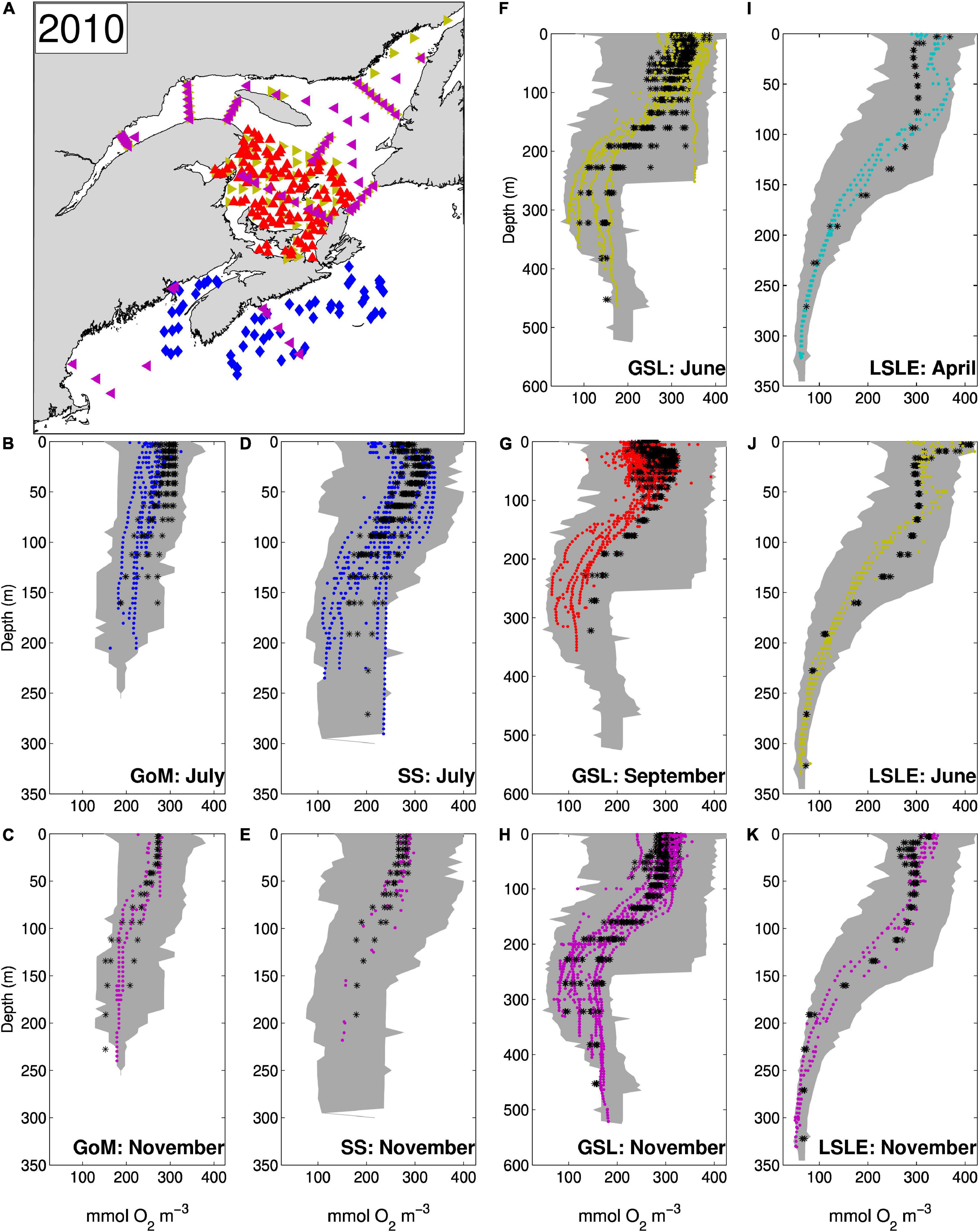
Figure 10. (A) Map showing the location of DO sampling in 2010 [the symbol colors indicate the month during which sampling occured, April (cyan), June (yellow), July (blue), September (red) and November (magenta)]. The observed (colored symbols) and simulated (black stars) DO profiles are compared for different regions shown in Figure 1, GoM (panels B,C), SS (panels D,E), GSL (panels F–H), and LSLE (panels I–K). The shaded area represents the range of observed values in the same regions over years 2008 to 2011.

FIGURE 11

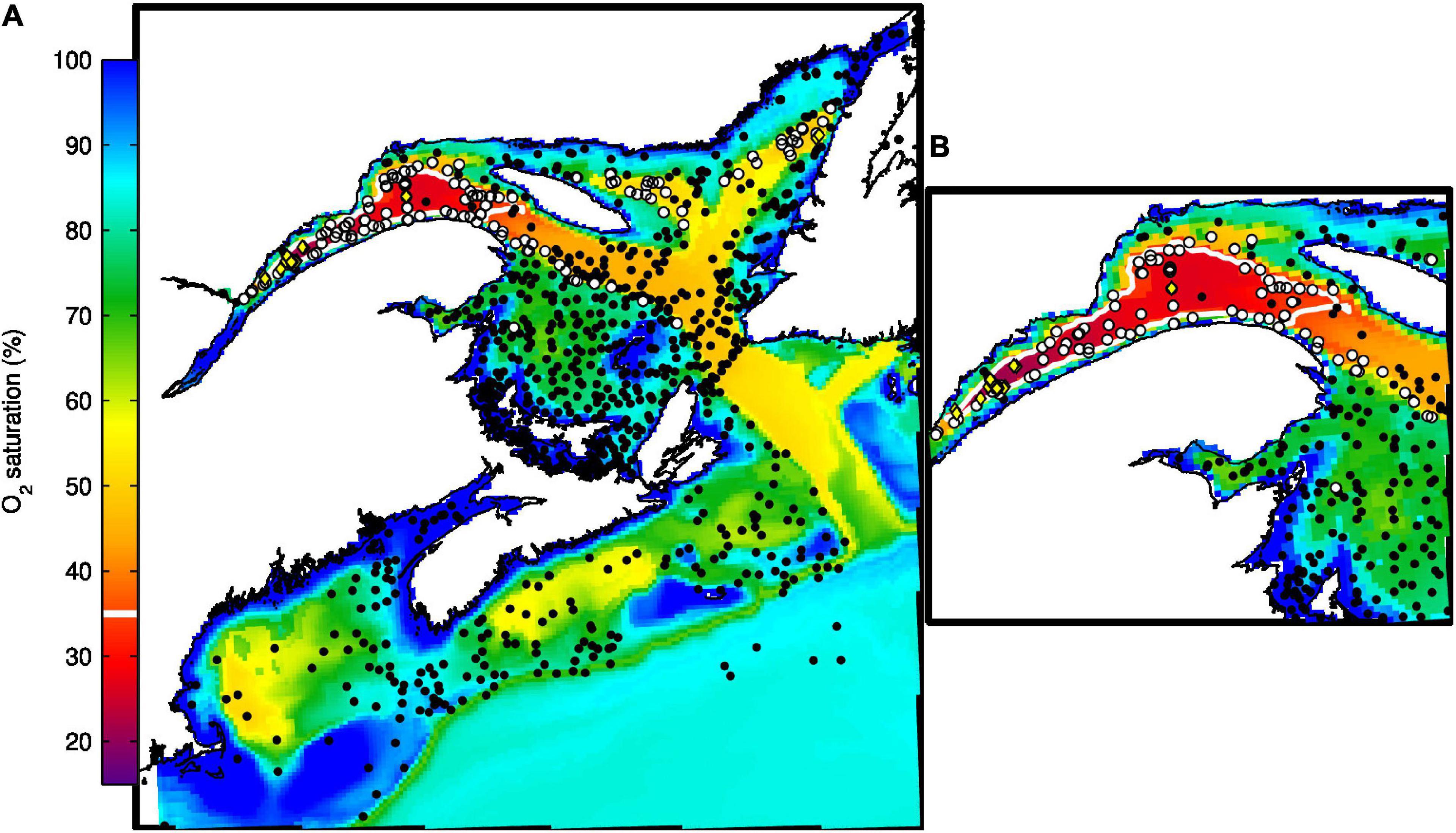
Figure 11. (A) Mean simulated bottom oxygen saturation for June and July of 2009 and 2010. Dots represent position of observations for the same months and years. White dots (observation) and line (simulation) correspond to saturation values smaller than 35%, while yellow diamonds correspond to saturation values smaller than 20%. Panel (B) presents an enlargement of the Lower St. Lawrence Estuary and Northwest Gulf of St. Lawrence regions.

Besides the LSLE hypoxic zone, the model reproduced many other observed features of the DO distribution, such as the horse shoe shape of the 35% saturation contour in the nwGSL (although our annual mean does not extend as far along the southern edge of the Laurentian Channel, Figure 11), and the minimum DO along the edge of the Scotian Shelf (see Figure 2 of Bianucci et al., 2016) and in some basins on the Scotian Shelf (Figure 11). Observed and simulated DO profiles in the GoM are also in good agreement (Figures 10B,C). The simulated DO seems to be a little high in July (Figure 10B) compared to observed profiles, although it remains within the values observed over a few years (shaded area).

Low DO saturation (below 35%) is also observed in the Esquiman and Anticosti Channels (white dots in Figure 11). Simulated DO saturation values are low in these channels but do not reach 35% (they rather oscillate around 40–45%). This is explained in part by a shallower depth in the model compared to reality. The comparison of bottom values is thus not made at the same depth. The amount of PON reaching the bottom might also be insufficient, due to a small amount of mesozooplankton, or to non-optimal PON sinking speed and remineralisation rates. The inclusion of a sediment box with slow release from the sediments rather than instant remineralisation could also improve DO concentrations and saturation levels in general, especially in regions where the productive period is short.

Our mean respiration rates in the water column (50–200 nmol O₂ L^–1 per day, Supplementary Figure 7) are similar to those estimated by Bourgault et al. (2012) (30–120 nmol O₂ L^–1 per day), although their vertical distribution differs. Bourgault et al. (2012) place minimum respiration rates in the cold intermediate layer, in accordance with the temperature dependency used for their pelagic respiration rate. Although we do include a temperature dependence of PON fragmentation rates, our minimum values are found in the deep layers in the eastern part of the GSL that receives a smaller amount of organic matter compared to other regions. However, high respiration rates are simulated in the LSLE and nwGSL near the bottom (Pointe-des-Monts area in Supplementary Figure 7) due to the greater accumulation of PON near the bottom in that region (Figures 9B,D). These respiration rates are, however, low compared to other estuarine systems (Fennel and Testa, 2019).

Carbonate System

In this section we evaluate the simulated air-sea CO₂ fluxes as well as pH and calcium carbonate saturation states at the bottom water that are particularly low in the LSLE (Mucci et al., 2011). Simulated air-sea CO₂ fluxes are compared with data reported in the literature. In the LSLE and GSL, air-sea CO₂ fluxes have been estimated by Dinauer and Mucci (2017). The LSLE is a source of atmospheric CO₂ in general due to the strong influence of freshwater inflow that carries organic matter into the LSLE where it is remineralized and leads to an increase in surface water pCO_2.. This process is counteracted during late spring and summer by the strong primary production taking place in the LSLE that consumes DIC and leads to low surface pCO₂ (Supplementary Figure 8) and a reversal of the flux. The range of simulated air-sea CO₂ flux calculated for the months of May to July (−3.1 ± 5.2 mmol C m^–2 d^–1, with values ranging between −43.8 to 26 mmol C m^–2 d^–1 over years 2010 to 2016) corresponds to the estimates of Dinauer and Mucci (2017) for the same months and years (0.8 ± 7.2 mmol C m^–2 d^–1, range −21.9 to 15.1 mmol C m^–2 d^–1). The means have opposite sign but are small in both cases. A negative sign represents CO₂ being taken up by the ocean, while a positive sign represents outgassing of CO₂ to the atmosphere. The difference in the mean can result from our earlier bloom timing in the LSLE (Figure 8G), to the fact that the model covers the entire area of the LSLE, as well as the entire three-months period each year, which is not the case with the field sampling.

In contrast to the LSLE, the GSL is a sink of atmospheric CO₂ in winter and during the spring bloom (April-May). Outgassing occurs afterwards as the sea surface warms (see flux reversal at the end of May in Supplementary Figure 8). On average, Dinauer and Mucci (2017) estimated that the GSL would be a weak sink (−1.2 ± 3.0 mmol C m^–2 d^–1, with values spatially ranging between −8.4 to 3.6 mmol C m^–2 d^–1). Here again, the model results show a similarly low mean (1.35 ± 6.5 mmol C m^–2 d^–1) but with a large range of fluxes (−43.8 to 17.8 mmol C m^–2 d^–1). The CO₂ fluxes calculated in the boxes NWGSL, CGSL, AS, EC and CA represented in Figure 9A were used to calculate the mean (rather than the GSL box of Figure 1) for a better comparison with the estimations of Dinauer and Mucci (2017) that do not cover the southern GSL.

The model also reproduces well the low pH in the Laurentian Channel (Figures 6D,H, 12A), and at the Shediac Station (7.7 to 7.9, Menu-Courey et al. (2019), see Figure 1 for the location of the Shediac Station). The model also reproduces the main features of bottom water aragonite saturation state. Most of the bottom waters of the GSL are undersaturated with respect to aragonite. This is also true for the shallower southern GSL where important remineralization of organic matter occurs, as mentioned previously. We do not have data for a direct comparison of aragonite saturation in the GoM but Wang et al. (2013) report aragonite saturation states below 1.3 in the deep part of the GoM, which corresponds to our simulated values (Figure 12B). The simulated values on the Scotian Shelf are, however, slightly low (Figure 12B).

FIGURE 12

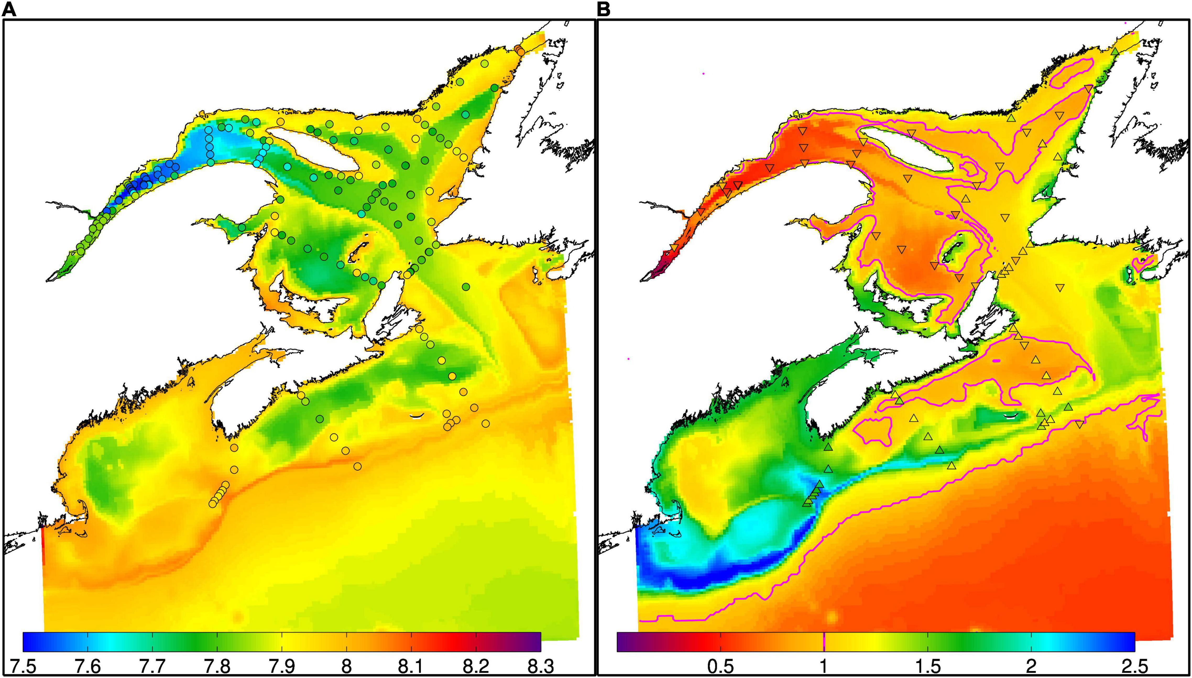
Figure 12. Simulated (background color) and observed (circles) bottom pH (A) and (triangles) aragonite saturation states (B) in October-November of 2014. The magenta line in panel B delimits the areas where simulated saturation states are below one. The upward-facing triangles indicate observed values above one, while the downward-facing triangle indicate that the observed values are below one.

Model Applications

The performance of the biogeochemical model was demonstrated above. We now use the model results to look at the impact of the circulation modes described in Lavoie et al. (2016) on the concentration and distribution of the biogeochemical variables. We also use the model to estimate the contribution of rivers in the total supply of nitrate to the surface layer of the LSLE.

Impact of Circulation Modes on the Seasonality of Biogeochemical Variables

Lavoie et al. (2016) described two mean seasonal circulation modes (winter-spring and summer-fall), different than the ones usually described as a function of surface stratification (spring-summer and fall-winter), and driven mainly by local and large-scale wind forcing. In winter and spring, a “semi-closed” circulation mode is present, with many strong gyres and reduced exchanges between the western and eastern GSL. The inflow at the Strait of Belle Isle and at Cabot Strait is stronger in winter, which, in the simulation, ultimately leads to an increased mean water level in the LSLE (see Figure 11 of Lavoie et al., 2016). The increased water level creates a west to east gradient that combines with the strong northwesterly winds to oppose the stronger inflow at the GSL’s bounding straits.

The nitrate flux from the St. Lawrence River is maximal in winter and spring, due to the combination of high runoff and high nitrate concentration (Figure 3B). The depth from which water is upwelled at the head of the Laurentian Channel is also maximal in winter (Saucier et al., 2009), which combined with a shoaling of the upper limit of Atlantic water (Galbraith, 2006), leads to upwelling of water with higher salinity and temperature (Belzile et al., 2016), higher nitrate concentration, and lower DO and pH than in summer. These two processes lead to the delivery of a large amount of nutrients to the LSLE when primary production is at a minimum. Because of the “semi-closed” configuration of the system at this time of the year, with its many gyres, the nutrients accumulate mostly in the LSLE and nwGSL. Some of this nutrient-enriched surface water also makes its way around the Gaspé Peninsula (Figure 5A). The downstream advection of nitrate directly from the LSLE or nwGSL towards the Scotian Shelf is comparatively low, but combined with the recycling of organic matter (see section “Ammonium Concentrations”), nitrate concentrations can reach about 6–8 mmol N m^–3 in the southern GSL in winter. These concentrations combined with strong transport at this time of the year lead to important nitrate transport out of the GSL at Cabot Strait, both observed and simulated (Figures 7A,E). In spring, increased river runoff and surface heat flux increase stratification, light availability increases and surface nutrients are used up by primary producers in most regions, except in the LSLE due to greater light limitation caused by turbid waters.

During summer, the transport at the GSL’s bounding straits is minimal, the northwest winds are weak and the westward coastal current along the northern coast of the GSL is stronger and often flows as far as the Saguenay fjord in the LSLE (Lavoie et al., 2016). The Anticosti gyre is not closed (more of a U shape), and the outflow of the St. Lawrence River remains close to the south shore of the LSLE. The circulation in the eastern GSL is weaker. Overall, there are fewer gyres present in the system in the second circulation mode. Primary production is still high in the LSLE and Gaspé Current during summer, due to the constant supply of nutrient by upwelling at the Laurentian Channel head. During this more “open” circulation mode, less regional retention is occurring and a larger part of the phytoplankton, zooplankton, and particulate and dissolved organic material produced in the LSLE and Gaspé Current are transported towards the Magdalen Shallow where they are recycled (Plourde and Runge, 1993; Zakardjian et al., 2000; Savenkoff et al., 2001; Figure 15 of Ouellet et al., 2013). This recycling leads to the high ammonium concentrations reported in section “Ammonium Concentrations” (up to 7 mmol N m^–3 depending on the year, Figures 5B,D), and low DO, pH and aragonite saturation compared to other relatively shallow regions (Figures 11, 12). The high ammonium concentration observed in late summer and early fall are then oxidized to nitrate, which will then be available for transport towards the Scotian Shelf. Outflow of inorganic nutrient and organic material also occurs along the southern edge of the Laurentian Channel and eventually flows into the deep channels and basins of the Scotian Shelf. Remineralization of this organic matter along the way leads to a nitrate maximum and a DO minimum along the shelf edge, from within the GSL down to the Gulf of Maine (Figure 11).

In summary, nutrients are made available through upwelling and river flux to the surface of the LSLE, nwGSL and partly to the southern GSL. As these nutrients are used up, the organic matter produced is transported towards the southern GSL, where it is recycled to nitrate that is transported towards the Scotian Shelf where it will be used up in spring. The combination of the dynamics of the planktonic system with the circulation modes over the year leads to a cascade that eventually bring the nutrients from far upstream, down to the Scotian Shelf and most likely as far as the GoM, through one or two transformation cycles.

Nitrate Sources and Relative Contribution of Rivers

The demonstrated skill of the coupled biogeochemical model and the inclusion of riverine input allows us to revisit important questions about nitrate sources in the system and their relative contribution. The main sources of nutrients to the GSL are the St. Lawrence River (which combines high runoff with high nutrient concentrations), inflow at the Strait of Belle Isle and Cabot Strait, and atmospheric deposition. The importance of each of these contributions to the GSL nutrient budget is investigated in a separate paper in preparation.

Here we compare the riverine input with the upwelling flux at the Laurentian Channel head. The latter is estimated as the mean flux through the base of the 6th layer, located at 46 m, averaged over the purple box displayed in Figure 1.

The St. Lawrence River represents a sizable nutrient contribution to the surface layers of the LSLE, depending on the time of the year. Using monthly mean concentrations and runoff at Quebec City (corresponding to the model input at this boundary) we obtain a nitrate flux of 288 mol N s^–1 (12.7 × 10⁴ tons y^–1). This is twice the flux of 5.7 × 10⁴ tons y^–1 estimated by Greisman and Ingram (1977) using a mean nitrate concentrations of 13 mmol N m^–3 in Lac St. Pierre and a mean runoff of 10,000 m³ s^–1. Their estimate is based on data sampled in June-July 1975. Our estimate is also higher than the estimate of Coote and Yeats (1979) of 8.4 × 10⁴ tons y^–1 who used annual means for nitrate concentration (14 mmol N m^–3) and runoff (13,000 m³ s^–1) at Quebec City. Our estimate is higher because we use monthly values, where the maximum runoff corresponds to the maximum nitrate concentration (30.6 mmol N m^–3 in April) and also because our annual mean nitrate concentration, based on more recent data, is higher (22.5 mmol N m^–3). Our mean runoff is similar at 11,000 m³ s^–1. The total nitrate contribution of all the rivers included in the model and that flow into the GSL is equal to 324 mol N s^–1 (14.3 × 10⁴ tons y^–1). The St. Lawrence River is clearly the main riverine contributor, supplying nearly 90% of nitrate from rivers.

Greisman and Ingram (1977) estimated that the St. Lawrence River contribution to the nitrate pool of the LSLE surface layer was less than 25% based on their June-July measurements. Using inverse modelling, Savenkoff et al. (2001) obtained a similar contribution, 18%, for the July to September period. However, Gilbert et al. (2007) estimated that in spring, when both nutrient concentration and runoff are at their maximum, this relative contribution could reach 50%. The other half would be supplied by the intense vertical mixing and upwelling at the Laurentian Channel head.

The model results are mostly in accordance with these estimates with a mean St. Lawrence River contribution of about 25% in summer (June to September) and a higher river contribution from late fall to early spring of about 36%. The minimum St. Lawrence River contributions were simulated in July 2012, August 2009, 2012, 2015, and 2016, and September 2014 (between 18 and 20%). The largest St. Lawrence River contribution was simulated in December 2010 (51%) and in March and April 2017 (42 and 45% respectively). Our mean winter-early spring riverine contribution is smaller than the 50% estimated by Gilbert et al. (2007) because even though the riverine flux increases, water that upwells at the head of the Laurentian Channel during this period also contains a greater amount of nutrients (see section “Impact of Circulation Modes on the Seasonality of Biogeochemical Variables”). The very large contribution in December 2010 (51%) is anomalous (the December average is 36%) and results from strong easterly winds that led to high water levels in the LSLE and reduced upwelling.

Conclusion

A new biogeochemical model of the GSL, based on LF05, but to which numerous additions/changes were made, including the addition of a dissolved oxygen and dissolved inorganic carbon components, was presented. Changes to LF05 were made in order to maintain the biogeochemical characteristics over multi-year runs. This is essential if we want to use the model to study the inter-annual variability and make climate projections. These important changes included the addition of nitrification, modification to the particulate organic matter sinking and fragmentation rates, and instantaneous remineralisation of part of the organic matter that reaches the sediments. The impact of these changes is discussed in more detail in the Supplementary Material. The model skill was demonstrated by a comparison with numerous data as well as with fluxes and budgets reported in the literature. The stability of the model is demonstrated by the good comparison with observations (up to 2017), many years after the model initialisation (2005). Annual and inter-annual variability are also specifically represented in Figures 7, 10.

The results highlight the importance of the remineralization of organic matter, partly imported from upstream regions, taking place in the southern Gulf. This process leads to high ammonium concentrations and low DO, pH and calcium carbonate saturation states for such a shallow region. The processes taking place in this region also contribute to a transformation loop that contributes to the transport of nutrients from the GSL to the Scotian Shelf and eventually to the GoM. Thus, the GSL does act as a nutrient trap as stated by Coote and Yeats (1979), with a nutrient increase as the water moves up towards the head of the Laurentian Channel, but it also represents a nutrient source to downstream regions. The transformation of ammonium into nitrate also maintains high primary productivity on the Magdalen Shallows, which support important fisheries. This process was not reproduced in LF05.

With the inclusion of many rivers, and their respective nitrate inputs, the model allowed us to calculate the relative contribution of rivers to the nitrate content of the mixed layer in the LSLE, compared to the upwelling at the head of the Laurentian Channel. Our estimates were similar to those estimated in the literature for the summer period. However, we showed that the river contribution was larger in winter and early spring, but not as much as had been previously estimated.

The model represents a tool that can be used to elucidate the complex functioning of the GSL ecosystem and answer different questions to support fisheries and ecosystem management. Two additional studies using this numerical model are under way to analyse the seasonal variability of the carbonate system, and the processes governing the interannual variability of primary production in the GSL. Next steps for model development include the addition of the effect of temperature on all biological processes to study the impact of climate change on the biogeochemical state of the system, the inclusion of a simple sediment model to represent the temporal delay in remineralization of sedimenting PON, and forcing with annually variable boundary conditions.

Data Availability Statement

The observations used in the paper are available through public repositories. The source code, boundary conditions and other databases as well as simulation raw data supporting the conclusions of this paper are very large and thus difficult to drop in a public repository. However, all are archived on the Fisheries and Oceans Canada servers and available on request without undue reservation.

Author Contributions

DL, MS, and JC conceived the project. JC helped with the coupling between NEMO and GSBM. YL implemented the oxygen module. JRC provided the carbonate system code that BB implemented into GSBM. MS and KA-S provided data and advice with the carbonate system. DG provided dissolved oxygen observational data. NL implement total alkalinity as a tracer. DL, NL, JC, and OR were responsible for the coupled model improvements. DL, NL and OR were responsible for the simulations and analysis. DL wrote the first draft of the manuscript. All authors provided feedback and contributed to the final manuscript.

Funding

The model development was financed by different programs and centers of expertise at Fisheries and Oceans Canada: the Aquatic Climate Change Adaptation Services Program (ACCASP), the Strategic Program for Ecosystem-based Research and Advice (SPERA), the Center of Expertise on Hydropower Impacts on Fish and Fish Habitat (CHIF), and the Centre for Ocean Model Development and Applications (COMDA).

Conflict of Interest

The authors declare that the research was conducted in the absence of any commercial or financial relationships that could be construed as a potential conflict of interest.

Publisher’s Note

All claims expressed in this article are solely those of the authors and do not necessarily represent those of their affiliated organizations, or those of the publisher, the editors and the reviewers. Any product that may be evaluated in this article, or claim that may be made by its manufacturer, is not guaranteed or endorsed by the publisher.

Acknowledgments

We are indebted to David Brickman for providing the code of the initial implementation of the NEMO model over the CANOPA domain, and for providing the open boundary conditions for the physical variables. We thank him and Adam Drozdowski for their help in coupling GSBM to NEMO. We also thank Serge Hebert for providing biogeochemical data in some of the Quebec Rivers. We thank Dominique Hamel for digging nitrate data in New Brunswick and Newfoundland rivers as well as Corinne Bourgault-Brunelle for digging biogeochemical data from the American rivers. We also thank Claude Savenkoff for providing the JGOFS data, Gary Maillet for providing nitrate data on the Newfoundland shelf for the preparation of boundary conditions, as well as Pierre Pepin for carbonate system data around Newfoundland. We thank Bertille Lefèvre for the validation of the simulated air-sea CO₂ fluxes in the St. Lawrence Estuary. Finally, we thank the two reviewers whose comments helped to improve the manuscript.

Supplementary Material

The Supplementary Material for this article can be found online at: https://www.frontiersin.org/articles/10.3389/fmars.2021.732269/full#supplementary-material

Abbreviations

AZMP, Atlantic Zone Monitoring Program; DIC, Dissolved Inorganic Carbon; DO, Dissolved Oxygen; DON, Dissolved Organic Nitrogen; GoM, Gulf of Maine; GSBM, Gulf of St. Lawrence Biogeochemical Model; GSL, Gulf of St. Lawrence; LP, Large Phytoplankton; LSLE, Lower St. Lawrence Estuary; MEZ, Mesozooplankton; MIZ, Microzooplankton; SP, Small Phytoplankton; NPZD, Nutrient-Phytoplankton-Zooplankton-Detritus; nwGSL, northwest Gulf of St. Lawrence; PON, Particulate Organic Nitrogen; TA, Total Alkalinity.

Footnotes

1. ^ https://www.ec.gc.ca/stl/
2. ^ https://dfo-mpo.gc.ca/
3. ^ https://ogsl.ca/en/home-slgo/
4. ^ https://www.bio.gc.ca/science/research-recherche/ocean/modelling-modelisation/oceanmod/oax-en.php

References

Al Azhar, M., Lachkar, Z., Lévy, M., and Smith, S. (2017). Oxygen minimum zone contrasts between the Arabian Sea and the Bay of Bengal implied by differences in remineralization depth. Geophys. Res. Lett. 44, 11,106–11,111. doi: 10.1002/2017GL075157

CrossRef Full Text | Google Scholar

Aumont, O., Ethé, C., Tagliabue, A., Bopp, L., and Gehlen, M. (2015). PISCES-v2: an ocean biogeochemical model for carbon and ecosystem studies. Geosci. Model Dev. 8, 2465–2513. doi: 10.5194/gmd-8-2465-2015

CrossRef Full Text | Google Scholar

Azetsu-Scott, K., Clarke, A., Falkner, K., Hamilton, J., Jones, E. P., Lee, C., et al. (2010). Calcium carbonate saturation states in the waters of the Canadian Arctic Archipelago and the Labrador Sea. J. Geophys. Res. 115:C11021. doi: 10.1029/2009JC005917

CrossRef Full Text | Google Scholar

Bailey, W. B. (1958). On the dominant flow in the Strait of Belle Isle. J. Fish. Res. Board Can. 15, 1163–1174. doi: 10.1139/f58-061

PubMed Abstract | CrossRef Full Text | Google Scholar

Baker, C. A., Henson, S. A., Cavan, E. L., Giering, S. L. C., Yool, A., Gehlen, M., et al. (2017). Slow-sinking particulate organic carbon in the Atlantic Ocean: magnitude, flux, and potential controls. Global Biogeochem. Cycles 31, 1051–1065. doi: 10.1002/2017GB005638

CrossRef Full Text | Google Scholar

Belzile, M., Galbraith, P. S., and Bourgault, D. (2016). Water renewals in the Saguenay Fjord. J. Geophys. Res. 121, 638–657. doi: 10.1002/2015jc011085

CrossRef Full Text | Google Scholar

Benson, B. B., and Krause, D. (1984). The concentration and isotopic fractionation of oxygen dissolved in fresh-water and seawater in equilibrium with the atmosphere. Limnol. Oceanogr. 29, 620–632. doi: 10.4319/lo.1984.29.3.0620

CrossRef Full Text | Google Scholar

Bianucci, L., Fennel, K., Chabot, D., Shackell, N., and Lavoie, D. (2016). Ocean biogeochemical models as management tools: a case study for Atlantic wolffish and declining oxygen. ICES J. Mar. Sci. 73, 263–274. doi: 10.1093/icesjms/fsv220

CrossRef Full Text | Google Scholar

Bourgault, D., and Koutitonsky, V. G. (1999). Real-time monitoring of the freshwater discharge at the head of the St. Lawrence Estuary. Atmos. Ocean 37, 203–220. doi: 10.1080/07055900.1999.9649626

CrossRef Full Text | Google Scholar

Bourgault, D., Cyr, F., Galbraith, P. S., and Pelletier, E. (2012). Relative importance of pelagic and sediment respiration in causing hypoxia in a deep estuary. J. Geophys. Res. 117:C08033. doi: 10.1029/2012JC007902

CrossRef Full Text | Google Scholar

Brennan, C. E., Blanchard, H., and Fennel, K. (2016). Putting temperature and oxygen thresholds of marine animals in context of environmental change: a regional perspective for the Scotian Shelf and Gulf of St. Lawrence. PLoS One 11:e0167411. doi: 10.1371/journal.pone.0167411

PubMed Abstract | CrossRef Full Text | Google Scholar

Brennan, C. E., Maps, F., Gentleman, W. C., Lavoie, D., Chassé, J., Plourde, S., et al. (2021). Ocean circulation changes drive shifts in Calanus abundance in North Atlantic right whale foraging habitat: a model comparison of cool and warm year scenarios. Prog. Oceanogr. 197:102629. doi: 10.1016/j.pocean.2021.102629

CrossRef Full Text | Google Scholar

Brickman, D., and Drozdowski, A. (2012). Development and validation of a regional shelf model for Maritime Canada based on the NEMO-OPA circulation model. Can. Tech. Rep. Hydrogr. Ocean Sci. 278:57.

Google Scholar

Brickman, D., and Petrie, B. (2003). Nitrate, silicate, and phosphate atlas for the Gulf of St. Lawrence. Can. Tech. Rep. Hydrogr. Ocean Sci. 231:152.

Google Scholar

Bugden, G. L. (1991). “Changes in the temperature-salinity characteristics of the deeper waters of the Gulf of St. Lawrence over the past several decades,” in The Gulf of St. Lawrence: Small Ocean or Big Estuary, ed. J.-C. Therriault (Ottawa, ON: Canadian Special Publication of Fisheries and Aquatic Sciences), 139–147.

Google Scholar

Buitenhuis, E., Le Quéré, C., Aumont, O., Beaugrand, G., Bunker, A., Hirst, A., et al. (2006). Biogeochemical fluxes through mesozooplankton. Global Biogeochem. Cycles 20:gb002511. doi: 10.1029/2005gb002511

CrossRef Full Text | Google Scholar

Claret, M., Galbraith, E. D., Palter, J. B., Bianchi, D., Fennel, K., Gilbert, D., et al. (2018). Rapid coastal deoxygenation due to ocean circulation shift in the northwest Atlantic. Nat. Clim. Change 8, 868–872. doi: 10.1038/s41558-018-0263-1

PubMed Abstract | CrossRef Full Text | Google Scholar

Coote, A. R., and Yeats, P. A. (1979). Distribution of nutrients in the Gulf of St. Lawrence. J. Fish. Res. Board Can. 36, 122–131. doi: 10.1139/f79-021

PubMed Abstract | CrossRef Full Text | Google Scholar

Cyr, F., Bourgault, D., Galbraith, P. S., and Gosselin, M. (2015). Turbulent nitrate fluxes in the Lower St. Lawrence Estuary, Canada. J. Geophys. Res. 120, 2308–2330. doi: 10.1002/2014jc010272

CrossRef Full Text | Google Scholar

de Lafontaine, Y., Demers, S., and Runge, J. (1991). “Pelagic food web interactions and productivity in the Gulf of St. Lawrence: a perspective,” in The Gulf of St. Lawrence: Small Ocean or Big Estuary, ed. J. C. Therriault (Ottawa, ON: Canadian Special Publication of Fisheries and Aquatic Sciences), 99–123.

Google Scholar

Devine, L., Kennedy, M. K., St-Pierre, I., Lafleur, C., Ouellet, M., and Bond, S. (2014). BioChem: the fisheries and oceans Canada database for biological and chemical data. Can. Tech. Rep. Fish. Aquat. Sci. 3073:40.

Google Scholar

Devine, L., Savenkoff, C., Vézina, A. F., Chanut, J.-P., Roy, S., Comeau, L., et al. (1997). Compilation des données biologiques et chimiques dans l’estuaire maritime du Saint-Laurent: programme COUPPB 1989, 1990 et 1991. Rapp. Stat. Can. Hydrogr. Sci. Océan. 150:103.

Google Scholar

DFO (2011a). Social, Economic, and Cultural Overview of the Quebec Region. Oceans, Habitat and Species at Risk Publication Series. Newfoundland and Labrador Region, No. 0007. St. John’s, NL: Fisheries and Oceans Canada Newfoundland and Labrador Region.

Google Scholar

DFO (2011b). Synopsis of the Social, Economic, and Cultural Overview of the Gulf of St. Lawrence. Oceans, Habitat and Species at Risk Publication Series. Newfoundland and Labrador Region, No. 0005. St. John’s, NL: Fisheries and Oceans Canada Newfoundland and Labrador Region.

Google Scholar

DFO (2020). Oceanographic Conditions in the Atlantic Zone in 2019. DFO Canadian Science Advisory Secretariat Science Advisory Report. 2020/028. St. John’s, NL: Newfoundland and Labrador.

Google Scholar

Dickson, A. G., Sabine, C. L., and Christian, J. R. (2007). Guide to Best Practices for Ocean CO₂ Measurements. PICES Special Publication, Vol. 3. Sidney, BC: North Pacific Marine Science Organization, 191.

Google Scholar

Dinauer, A., and Mucci, A. (2017). Spatial variability in surface-water pCO₂ and gas exchange in the world’s largest semi-enclosed estuarine system: St. Lawrence Estuary (Canada). Biogeosciences 14, 3221–3237. doi: 10.5194/bg-14-3221-2017

CrossRef Full Text | Google Scholar

Fasham, M. J. R., and Evans, G. T. (1995). The use of optimization techniques to model marine ecosystem dynamics at the JGOFS station at 47 degrees N 20 degrees W. Philos. Trans. R. Soc. Lond. B 348, 203–209. doi: 10.1098/rstb.1995.0062

CrossRef Full Text | Google Scholar

Fennel, K., and Testa, J. M. (2019). Biogeochemical controls on coastal hypoxia. Annu. Rev. Mar. Sci. 11, 105–130. doi: 10.1146/annurev-marine-010318-095138

PubMed Abstract | CrossRef Full Text | Google Scholar

Fournier, R. O., Marra, J., Bohrer, R., and Vandet, M. (1977). Plankton dynamics and nutrient enrichment of Scotian Shelf. J. Fish. Res. Board Can. 34, 1004–1018. doi: 10.1139/f77-153

PubMed Abstract | CrossRef Full Text | Google Scholar

Fuentes-Yaco, C., Vezina, A. F., Larouche, P., Gratton, Y., and Gosselin, M. (1997). Phytoplankton pigment in the Gulf of St. Lawrence, Canada, as determined by the coastal zone color scanner. Part II: multivariate analysis. Cont. Shelf Res. 17, 1441–1459. doi: 10.1016/s0278-4343(97)00022-8

CrossRef Full Text | Google Scholar

Galbraith, P. S. (2006). Winter water masses in the Gulf of St. Lawrence. J. Geophys. Res. 111:C06022. doi: 10.1029/2005JC003159

CrossRef Full Text | Google Scholar

Galbraith, P. S., Chassé, J., Caverhill, C., Nicot, P., Gilbert, D., Pettigrew, B., et al. (2016). Physical Oceanographic Conditions in the Gulf of St. Lawrence in 2015. DFO Canadian Science Advisory Secretaria Research Document 2016/056. Ottawa ON: Fisheries and Oceans Canada Canadian Science Advisory Secretariat.

Google Scholar

Galbraith, P. S., Larouche, P., Chasse, J., and Petrie, B. (2012). Sea-surface temperature in relation to air temperature in the Gulf of St. Lawrence: interdecadal variability and long term trends. Deep Sea Res. II 77–80, 10–20. doi: 10.1016/j.dsr2.2012.04.001

CrossRef Full Text | Google Scholar

García, H. E., and Gordon, L. I. (1992). Oxygen solubility in seawater: better fitting equations. Limnol. Oceanogr. 37, 1307–1312. doi: 10.4319/lo.1992.37.6.1307

CrossRef Full Text | Google Scholar

Garcia, H. E., Locarnini, R. A., Boyer, T. P., Antonov, J. I., Baranova, O. K., Zweng, M. M., et al. (2010a). World Ocean Atlas 2009: Dissolved Oxygen, Apparent Oxygen Utilization, and Oxygen Saturation. NOAA Atlas NESDIS 70, Vol. 3. Washington, DC: U.S. Government Printing Office.

Google Scholar

Garcia, H. E., Locarnini, R. A., Boyer, T. P., Antonov, J. I., Zweng, M. M., Baranova, O. K., et al. (2010b). World Ocean Atlas 2009: Nutrients (phosphate, nitrate, silicate). NOAA Atlas NESDIS 71, Vol. 4. Washington, DC: U.S. Government Printing Office.

Google Scholar

Gaudet, T., and Leger, S. (2011). Oceans, Habitat and Species at Risk Publication Series, Newfoundland and Labrador Region, No. 0006. St. John’s, NL: Fisheries and Oceans Canada Newfoundland and Labrador Region.

Google Scholar

Gilbert, D. (2004). “Propagation of temperature signals along the northwest Atlantic continental shelf edge and into the Laurentian Channel,” in Proceedings of the ICES Annual Science Conference, Vigo.

Google Scholar

Gilbert, D., Chabot, D., Archambault, P., Rondeau, B., and Hébert, S. (2007). Appauvrissement en oxygène dans les eaux profondes du Saint-Laurent marin: causes possibles et impacts écologiques. Le Nat. Can. 131, 67–75.

Google Scholar

Gilbert, D., Sundby, B., Gobeil, C., Mucci, A., and Tremblay, G.-H. (2005). A seventy-two-year record of diminishing deep-water oxygen in the St. Lawrence estuary: the northwest Atlantic connection. Limnol. Oceanogr. 50, 1654–1666. doi: 10.4319/lo.2005.50.5.1654

CrossRef Full Text | Google Scholar

Greenan, B. J. W., Shackell, N. L., Ferguson, K., Greyson, P., Cogswell, A., Brickman, D., et al. (2019). Climate change vulnerability of American lobster fishing communities in Atlantic Canada. Front. Mar. Sci. 6:579. doi: 10.3389/fmars.2019.00579

CrossRef Full Text | Google Scholar

Greisman, P., and Ingram, G. (1977). Nutrient distribution in the St. Lawrence estuary. J. Fish. Res. Board Can. 34, 2117–2123.

Google Scholar

Haigh, S. P., Denman, K. L., and Hsieh, W. W. (2001). Simulation of the planktonic ecosystem response to pre- and post-1976 forcing in an isopycnic model of the North Pacific. Can. J. Fish. Aquat. Sci. 58, 703–722. doi: 10.1139/f01-010

PubMed Abstract | CrossRef Full Text | Google Scholar

Head, E. J. H., and Pepin, P. (2010). Monitoring changes in phytoplankton abundance and composition in the Northwest Atlantic: a comparison of results obtained by continuous plankton recorder sampling and colour satellite imagery. J. Plankton Res. 32, 1649–1660. doi: 10.1093/plankt/fbq120

CrossRef Full Text | Google Scholar

Henson, S. A., Dunne, J. P., and Sarmiento, J. L. (2009). Decadal variability in North Atlantic phytoplankton blooms. J. Geophys. Res. 114:C04013. doi: 10.1029/2008JC005139

CrossRef Full Text | Google Scholar

Hu, Z.-Z., Kumar, A., Huang, B., Xue, Y., Wang, W., and Jha, B. (2011). Persistent atmospheric and oceanic anomalies in the North Atlantic from summer 2009 to summer 2010. J. Clim. 24, 5812–5830. doi: 10.1175/2011jcli4213.1

CrossRef Full Text | Google Scholar

Hudon, C., Gagnon, P., Rondeau, M., Hebert, S., Gilbert, D., Hill, B., et al. (2017). Hydrological and biological processes modulate carbon, nitrogen and phosphorus flux from the St. Lawrence River to its estuary (Quebec, Canada). Biogeochemistry 135, 251–276. doi: 10.1007/s10533-017-0371-4

CrossRef Full Text | Google Scholar

Ingram, R. G. (1983). Vertical mixing at the head of the Laurentian Channel. Estuar. Coast. Shelf Sci. 16, 333–338. doi: 10.1016/0272-7714(83)90150-6

CrossRef Full Text | Google Scholar

Jin, X., Najjar, R. G., Louanchi, F., and Doney, S. C. (2007). A modeling study of the seasonal oxygen budget of the global ocean. J. Geophys. Res. 112:C05017. doi: 10.1029/2006JC003731

CrossRef Full Text | Google Scholar

Jolliff, J. K., Kindle, J. C., Shulman, I., Penta, B., Friedrichs, M. A. M., Helber, R., et al. (2009). Summary diagrams for coupled hydrodynamic-ecosystem model skill assessment. J. Mar. Syst. 76, 64–82. doi: 10.1016/j.jmarsys.2008.05.014

CrossRef Full Text | Google Scholar

Jutras, M., Dufour, C. O., Mucci, A., Cyr, F., and Gilbert, D. (2020). Temporal changes in the causes of the observed oxygen decline in the St. Lawrence Estuary. J. Geophys. Res. 125:e2020JC016577.

Google Scholar

Kawamiya, M., Kishi, M. J., Yamanaka, Y., and Suginohara, N. (1995). An ecological-physical coupled model applied to station Papa. J. Oceanogr. 51, 635–664. doi: 10.1007/bf02235457

CrossRef Full Text | Google Scholar

Kawamiya, M., Kishi, M., Yamanaka, Y., and Suginohara, N. (1997). Obtaining reasonable results in different oceanic regimes with the same ecological-physical coupled model. J. Oceanogr. 53, 397–402.

Google Scholar

Key, R. M., Olsen, A., van Heuven, S., Lauvset, S. K., Velo, A., Lin, X., et al. (2015). Global Ocean Data Analysis Project, Version 2 (GLODAPv2). Analysis Center, Oak Ridge National Laboratory. Washington, DC: US Department of Energy.

Google Scholar

Kortzinger, A., Hedges, J. I., and Quay, P. D. (2001). Redfield ratios revisited: removing the biasing effect of anthropogenic CO2. Limnol. Oceanogr. 46, 964–970. doi: 10.4319/lo.2001.46.4.0964

CrossRef Full Text | Google Scholar

Kriest, I., and Oschlies, A. (2015). MOPS-1.0: modelling the regulation of the global oceanic nitrogen budget by marine biogeochemical processes. Geosci. Model Dev. Discuss. 8, 1945–2010. doi: 10.5194/gmdd-8-1945-2015

CrossRef Full Text | Google Scholar

Kriest, I., Oschlies, A., and Khatiwala, S. (2012). Sensitivity analysis of simple global marine biogeochemical models. Global Biogeochem. Cycles 26:GB2029. doi: 10.1029/2011gb004072

CrossRef Full Text | Google Scholar

Laliberte, J., Larouche, P., Devred, E., and Craig, S. (2018). Chlorophyll-a concentration retrieval in the optically complex waters of the St. Lawrence Estuary and Gulf using principal component analysis. Remote Sens. Basel 10:265. doi: 10.3390/rs10020265

CrossRef Full Text | Google Scholar

Lambert, N., Chassé, J., Perrie, W., Long, Z., Guo, L., and Morrison, J. (2013). Projection of future river runoffs in Eastern Atlantic Canada from global and regional climate models. Can. Tech. Rep. Hydrogr. Ocean Sci. 288:34.

Google Scholar

Lavoie, D., Chassé, J., Simard, Y., Lambert, N., Galbraith, P. S., Roy, N., et al. (2016). Large-scale atmospheric and oceanic control on krill transport into the St. Lawrence Estuary evidenced with three-dimensional numerical modelling. Atmos. Ocean 54, 299–325. doi: 10.1080/07055900.2015.1082965

CrossRef Full Text | Google Scholar

Lavoie, D., Gilson, G., Chassé, J., Lambert, N., Brunelle, C. B., Starr, M., et al. (2017). Impacts of freshwater flow regulation of Quebec’s large rivers on the physical environment and krill transport in the Gulf of St. Lawrence and on the Scotian Shelf. Can. Tech. Rep. Hydrogr. Ocean Sci. 318:101.

Google Scholar

Lavoie, D., Lambert, N., and Gilbert, D. (2019). Projections of future trends in biogeochemical conditions in the Northwest Atlantic using CMIP5 Earth System Models. Atmos. Ocean 57, 18–40. doi: 10.1080/07055900.2017.1401973

CrossRef Full Text | Google Scholar

Lavoie, D., Macdonald, R. W., and Denman, K. L. (2009). Primary productivity and export fluxes on the Canadian shelf of the Beaufort Sea: a modelling study. J. Mar. Syst. 75, 17–32. doi: 10.1016/j.jmarsys.2008.07.007

CrossRef Full Text | Google Scholar

Lavoie, D., Simard, Y., and Saucier, F. J. (2000). Aggregation and dispersion of krill at channel heads and shelf edges: the dynamics in the Saguenay-St. Lawrence Marine Park. Can. J. Fish. Aquat. Sci. 57, 1853–1869. doi: 10.1139/f00-138

PubMed Abstract | CrossRef Full Text | Google Scholar

Lavoie, D., Starr, M., Chassé, J., Gilbert, D., Chabot, D., and Lambert, N. (2015). “The gulf of St. Lawrence biogeochemical model: a tool to study the evolution of hypoxic conditions and other habitat changes,” in Proceedings of the ICES CM 2015/R:14: ICES ASC 2015, Copenhagen.

Google Scholar

Lavoie, D., Starr, M., Zakardjian, B., and Larouche, P. (2008). Identification of Ecologically and Biologically Significant Areas (EBSA) in the Estuary and Gulf of St. Lawrence : Primary Production. DFO Canadian Science Advisory Secretariat Research Document. 2007/079. Ottawa, ON: Fisheries and Oceans Canada Canadian Science Advisory Secretariat.

Google Scholar

Le Fouest, V., Zakardjian, B., and Saucier, F. J. (2010). Plankton ecosystem response to freshwater-associated bulk turbidity in the subarctic Gulf of St. Lawrence (Canada): a modelling study. J. Mar. Syst. 81, 75–85. doi: 10.1016/j.jmarsys.2009.12.003

CrossRef Full Text | Google Scholar

Le Fouest, V., Zakardjian, B., Saucier, F. J., and Çizmeli, S. A. (2006). Application of SeaWIFS- and AVHRR-derived data for mesoscale and regional validation of a 3-D high-resolution physical-biological model of the Gulf of St. Lawrence (Canada). J. Mar. Syst. 60, 30–50. doi: 10.1016/j.jmarsys.2005.11.008

CrossRef Full Text | Google Scholar

Le Fouest, V., Zakardjian, B., Saucier, F. J., and Starr, M. (2005). Seasonal versus synoptic variability in planktonic production in a high-latitude marginal sea: the Gulf of St. Lawrence (Canada). J. Geophys. Res. 110:C09012. doi: 10.1029/2004JC002423

CrossRef Full Text | Google Scholar

Legendre, L. (1971). Production primaire dans la Baie des Chaleurs (Golfe du Saint-Laurent). Nat. Can. 98, 743–773.

Google Scholar

Lesage, V., Gosselin, J.-F., Lawson, J. W., McQuinn, I., Moors-Murphy, H., Plourde, S., et al. (2018). Habitats important to blue whales (Balaenoptera musculus) in the western North Atlantic. DFO Canadian Science Advisory Secretariat Research Document 2016/080. Ottawa, ON: Fisheries and Oceans Canada Canadian Science Advisory Secretariat.

Google Scholar

Levasseur, M., Fortier, L., Therriault, J. C., and Harrison, P. J. (1992). Phytoplankton dynamics in a coastal jet frontal region. Mar. Ecol. Prog. Ser. 86, 283–295. doi: 10.3354/meps086283

CrossRef Full Text | Google Scholar

Levasseur, M., Therriault, J. C., and Legendre, L. (1984). Hierarchical control of phytoplankton succession by physical factors. Mar. Ecol. Prog. Ser. 19, 211–222. doi: 10.3354/meps019211

CrossRef Full Text | Google Scholar

Loder, J. W., Han, G., Galbraith, P. S., Chassé, J., and van der Baaren, A. (2013). Aspects of climate change in the Northwest Atlantic off Canada. Can. Tech. Rep. Fish. Aquat. Sci. 3045:190.

Google Scholar

Lucotte, M., Hillaire-Marcel, C., and Louchouarn, P. (1991). First-order organic carbon budget in the St-Lawrence Lower Estuary from ¹³C data. Estuar. Coast. Shelf Sci. 32, 297–312. doi: 10.1016/0272-7714(91)90022-4

CrossRef Full Text | Google Scholar

Lueker, T. J., Dickson, A. G., and Keeling, C. D. (2000). Ocean pCO₂ calculated from dissolved inorganic carbon, alkalinity, and equations for K₁ and K₂: validation based on laboratory measurements of CO₂ in gas and seawater at equilibrium. Mar. Chem. 70, 105–119. doi: 10.1016/S0304-4203(00)00022-0

CrossRef Full Text | Google Scholar

Madec, G. (2012). NEMO Ocean Engine. Note du Pôle de modélisation, Vol. 27. Guyancourt: de l’Institut Pierre-Simon Laplace.

Google Scholar

Madec, G., Delecluse, P., Imbard, M., and Lévy, C. (1998). OPA 8.1 Ocean General Circulation Model reference manual. Note du Pôle de modélisation, Vol. 11. Guyancourt: de l’Institut Pierre-Simon Laplace.

Google Scholar

Maps, F., Plourde, S., McQuinn, I. H., St-Onge-Drouin, S., Lavoie, D., Chasse, J., et al. (2015). Linking acoustics and finite-time Lyapunov exponents reveals areas and mechanisms of krill aggregation within the Gulf of St. Lawrence, eastern Canada. Limnol. Oceanogr. 60, 1965–1975. doi: 10.1002/lno.10145

CrossRef Full Text | Google Scholar

Maps, F., Zakardjian, B. A., Plourde, S., and Saucier, F. J. (2011). Modeling the interactions between the seasonal and diel migration behaviors of Calanus finmarchicus and the circulation in the Gulf of St. Lawrence (Canada). J. Mar. Syst. 88, 183–202.

Google Scholar

Mei, Z.-P., Saucier, F. J., Le Fouest, V., Zakardjian, B., Sennville, S., Xie, H., et al. (2010). Modeling the timing of spring phytoplankton bloom and biological production of the Gulf of St. Lawrence (Canada): effects of colored dissolved organic matter and temperature. Cont. Shelf Res. 30, 2027–2042. doi: 10.1016/j.csr.2010.10.003

CrossRef Full Text | Google Scholar

Menu-Courey, K., Noisette, F., Piedalue, S., Daoud, D., Blair, T., Blier, P. U., et al. (2019). Energy metabolism and survival of the juvenile recruits of the American lobster (Homarus americanus) exposed to a gradient of elevated seawater pCO2. Mar. Environ. Res. 143, 111–123. doi: 10.1016/j.marenvres.2018.10.002

PubMed Abstract | CrossRef Full Text | Google Scholar

Mills, E. L., and Fournier, R. O. (1979). Fish production and the marine ecosystems of the Scotian shelf. East. Can. Mar. Biol. 54, 101–108. doi: 10.1007/Bf00386589

CrossRef Full Text | Google Scholar

Mousseau, L., Legendre, L., and Fortier, L. (1996). Dynamics of size-fractionated phytoplankton and trophic pathways on the Scotian shelf and at the shelf break, northwest Atlantic. Aquat. Microb. Ecol. 10, 149–163. doi: 10.3354/Ame010149

CrossRef Full Text | Google Scholar

Mucci, A., Starr, M., Gilbert, D., and Sundby, B. (2011). Acidification of lower St. Lawrence Estuary bottom waters. Atmos. Ocean 49, 206–218. doi: 10.1080/07055900.2011.599265

CrossRef Full Text | Google Scholar

Nicot, P. (2013). Modélisation et Analyses de Sensibilité des Conditions Hypoxiques aux Apports Fluviaux en Nitrate dans l’estuaire et le Golfe du Saint-Laurent. Master degree. Rimouski, QC: Université du Québec à Rimouski.

Google Scholar

Ohashi, K., and Sheng, J. (2018). Study of Atlantic salmon post-smolt movement in the Gulf of St. Lawrence using an individual-based model. Reg. Stud. Mar. Sci 24, 13–132. doi: 10.1016/j.rsma.2018.08.012

CrossRef Full Text | Google Scholar

Olsen, A., Key, R. M., van Heuven, S., Lauvset, S. K., Velo, A., Lin, X. H., et al. (2016). The global ocean data analysis project version 2 (GLODAPv2) – an internally consistent data product for the world ocean. Earth Syst. Sci. Data 8, 297–323. doi: 10.5194/essd-8-297-2016

CrossRef Full Text | Google Scholar

O’Reilly, J. E., and Busch, D. A. (1984). Phytoplankton primary production on the northwestern Atlantic shelf. Rapp. P.-v. Réun. Cons. int. Explor. Mer. 183, 255–268. doi: 10.1016/j.ecss.2014.12.047

CrossRef Full Text | Google Scholar

Ouellet, P., Bui, A. O. V., Lavoie, D., Chassé, J., Lambert, N., Ménard, N., et al. (2013). Seasonal distribution, abundance, and growth of larval capelin (Mallotus villosus) and the role of the lower estuary (Gulf of St. Lawrence, Canada) as a nursery area. Can. J. Fish. Aquat. Sci. 70, 1508–1530. doi: 10.1139/cjfas-2013-0227

PubMed Abstract | CrossRef Full Text | Google Scholar

Pellerin, G., Lefaivre, L., Houtekamer, P., and Girard, C. (2003). Increasing the horizontal resolution of ensemble forecasts at CMC. Nonlinear Proc. Geoph. 10, 463–468. doi: 10.5194/npg-10-463-2003

CrossRef Full Text | Google Scholar

Peterson, I., Greenan, B., Gilbert, D., and Hebert, D. (2017). Variability and wind forcing of ocean temperature and thermal fronts in the Slope Water region of the Northwest Atlantic. J. Geophys. Res. 122, 7325–7343. doi: 10.1002/2017JC012788

CrossRef Full Text | Google Scholar

Petrie, B., and Yeats, P. (2000). Annual and interannual variability of nutrients and their estimated fluxes in the Scotian Shelf, Gulf of Maine region. Can. J. Fish. Aquat. Sci. 57, 2536–2546. doi: 10.1139/f00-235

PubMed Abstract | CrossRef Full Text | Google Scholar

Plourde, S., and Runge, J. A. (1993). Reproduction of the planktonic copepod Calanus finmarchicus in the lower St. Lawrence Estuary: relation to the cycle of phytoplankton production and evidence for a Calanus pump. Mar. Ecol. Prog. Ser. 102, 217–227. doi: 10.3354/meps095217

CrossRef Full Text | Google Scholar

Plourde, S., Starr, M., Devine, L., St-Pierre, J.-F., St-Amand, L., Joly, P., et al. (2014). Chemical and Biological Oceanographic Conditions in the Estuary and Gulf of St. Lawrence During 2011 and 2012. DFO Canadian Science Advisory Secretariat Research Document 2014/049. Montreal, QC: Fisheries and Oceans Canada.

Google Scholar

Roy, S., Blouin, F., Jacques, A., and Therriault, J. C. (2008). Absorption properties of phytoplankton in the Lower Estuary and Gulf of St. Lawrence (Canada). Can. J. Fish. Aquat. Sci. 65, 1721–1737. doi: 10.1039/F08-089

CrossRef Full Text | Google Scholar

Roy, S., Sundby, B., Vézina, A. F., and Legendre, L. (2000). A Canadian JGOFS process study in the Gulf of St. Lawrence. introduction. Deep Sea Res. II Top. Stud. Oceanogr. 47, 377–384. doi: 10.1016/S0967-0645(99)00111-3

CrossRef Full Text | Google Scholar

Saucier, F. J., Roy, F., Gilbert, D., Pellerin, P., and Ritchie, H. (2003). Modeling the formation and circulation processes of water masses and sea ice in the Gulf of St. Lawrence, Canada. J. Geophys. Res. 108:3269. doi: 10.1029/2000jc000686

CrossRef Full Text | Google Scholar

Saucier, F. J., Roy, F., Senneville, S., Smith, G., Lefaivre, D., Zakardjian, B., et al. (2009). Modélisation de la circulation dans l’estuaire et le golfe du Saint-Laurent en réponse aux variations du débit d’eau douce et des vents. Rev. Sci. Eau 22, 159–176. doi: 10.7202/037480ar

PubMed Abstract | CrossRef Full Text | Google Scholar

Savenkoff, C., Vezina, A. F., Packard, T. T., Silverberg, N., Therriault, J. C., Chen, W., et al. (1996). Distributions of oxygen, carbon, and respiratory activity in the deep layer of the Gulf of St. Lawrence and their implications for the carbon cycle. Can. J. Fish. Aquat. Sci. 53, 2451–2465. doi: 10.1139/f96-198

PubMed Abstract | CrossRef Full Text | Google Scholar

Savenkoff, C., Vezina, A. F., Roy, S., Klein, B., Lovejoy, C., Therriault, J. C., et al. (2000). Export of biogenic carbon and structure and dynamics of the pelagic food web in the Gulf of St. Lawrence Part 1. Seasonal variations. Deep Sea Res. II 47, 585–607. doi: 10.1016/s0967-0645(99)00119-8

CrossRef Full Text | Google Scholar

Savenkoff, C., Vezina, A. F., Smith, P. C., and Han, G. (2001). Summer transports of nutrients in the Gulf of St. Lawrence estimated by inverse modelling. Estuar. Coast. Shelf Sci. 52, 565–587. doi: 10.1006/ecss.2001.0774

CrossRef Full Text | Google Scholar

Sévigny, J. M., Sinclair, M., El-Sabh, M. I., Poulet, S., and Coote, A. (1979). Summer plankton distributions associated with the physical and nutrient properties of the Northwestern Gulf of St. Lawrence. J. Fish. Res. Board Can. 36, 187–203. doi: 10.1139/f79-029

PubMed Abstract | CrossRef Full Text | Google Scholar

Shadwick, E. H., Thomas, H., Azetsu-Scott, K., Greenan, B. J. W., Head, E., and Horne, E. (2011). Seasonal variability of dissolved inorganic carbon and surface water pCO₂ in the Scotian Shelf region of the Northwestern Atlantic. Mar. Chem. 124, 23–37. doi: 10.1016/j.marchem.2010.11.004

CrossRef Full Text | Google Scholar

Sibert, V., Zakardjian, B., Gosselin, M., Starr, M., Senneville, S., and LeClainche, Y. (2011). 3D bio-physical model of the sympagic and planktonic productions in the Hudson Bay system. J. Mar. Syst. 88, 401–422. doi: 10.1016/j.jmarsys.2011.03.014

CrossRef Full Text | Google Scholar

Siegel, D. A., Doney, S. C., and Yoder, J. A. (2002). The North Atlantic spring phytoplankton bloom and Sverdrup’s critical depth hypothesis. Science 296, 730–733. doi: 10.1126/science.1069174

PubMed Abstract | CrossRef Full Text | Google Scholar

Signorini, S. R., McClain, C. R., Christian, J. R., and Wong, C. S. (2001). Seasonal and interannual variability of phytoplankton, nutrients, TCO₂, pCO₂, and O₂ in the eastern subarctic Pacific (ocean weather station Papa). J. Geophys. Res 106, 31197–31215. doi: 10.1029/2000jc000343

CrossRef Full Text | Google Scholar

Silverberg, N., Sundby, B., Mucci, A., Zhong, S., Arakaki, T., Hall, P., et al. (2000). Remineralization of organic carbon in eastern Canadian continental margin sediments. Deep Sea Res. II 47, 699–731. doi: 10.1016/S0967-0645(99)00123-X

CrossRef Full Text | Google Scholar

Simard, Y., and Lavoie, D. (1999). The rich krill aggregation of the Saguenay - St. Lawrence Marine Park: hydroacoustic and geostatistical biomass estimates, structure, variability, and significance for whales. Can. J. Fish. Aquat. Sci. 56, 1182–1197. doi: 10.1139/f99-063

PubMed Abstract | CrossRef Full Text | Google Scholar

Simard, Y., Roy, N., Giard, S., and Aulanier, F. (2019). North Atlantic right whale shift to the Gulf of St. Lawrence in 2015, revealed by long-term passive acoustics. Endang. Species Res. 40, 271–284. doi: 10.3354/esr01005

CrossRef Full Text | Google Scholar

Sinclair, M., El-Sabh, M., and Brindle, J. R. (1976). Seaward nutrient transport in the lower St Lawrence estuary. J. Fish. Res. Board Can. 33, 1271–1277. doi: 10.1139/f76-163

PubMed Abstract | CrossRef Full Text | Google Scholar

Starr, M., St-Amand, L., Devine, L., Bérard-Therriault, L., and Galbraith, P. S. (2004). State of Phytoplankton in the Estuary and Gulf of St. Lawrence during 2003. Canadian Science Advisory Secretariat Document 2004/123. Ottawa, ON: Fisheries and Oceans.

Google Scholar

Steven, D. M. (1974). Primary and Secondary Production in the Gulf of St. Lawrence. Marine Science Centre Manuscript, Report No. 26. Montreal, QC: McGill University.

Google Scholar

Stortini, C. H., Chabot, D., and Shackell, N. L. (2017). Marine species in ambient low-oxygen regions subject to double jeopardy impacts of climate change. Glob. Chang. Biol. 23, 2284–2296. doi: 10.1111/gcb.13534

PubMed Abstract | CrossRef Full Text | Google Scholar

Therriault, J. C., and Lacroix, G. (1976). Nutrients, chlorophyll, and internal tides in the St. Lawrence estuary. J. Fish. Res. Board Can. 33, 2747–2757. doi: 10.1139/f76-326

PubMed Abstract | CrossRef Full Text | Google Scholar

Therriault, J. C., and Levasseur, M. (1985). Control of phytoplankton production in the lower St. Lawrence Estuary: light and freshwater runoff. Nat. Can. 112, 77–96.

Google Scholar

Tian, R. C., Vezina, A. F., Starr, M., and Saucier, F. (2001). Seasonal dynamics of coastal ecosystems and export production at high latitudes: a modeling study. Limnol. Oceanogr. 46, 1845–1859. doi: 10.4319/lo.2001.46.8.1845

CrossRef Full Text | Google Scholar

Tian, R. C., Vézina, A., Legendre, L., Ingram, R. G., Klein, B., Packard, T., et al. (2000). Effects of pelagic food-web interactions and nutrient remineralization on the biogeochemical cycling of carbon: a modeling approach. Deep Sea Res. II 47, 637–662. doi: 10.1016/S0967-0645(99)00121-6

CrossRef Full Text | Google Scholar

Tremblay, J. E., Legendre, L., Klein, B., and Therriault, J. C. (2000). Size-differential uptake of nitrogen and carbon in a marginal sea (Gulf of St. Lawrence, Canada): significance of diel periodicity and urea uptake. Deep Sea Res. II 47, 489–518. doi: 10.1016/s0967-0645(99)00116-2

CrossRef Full Text | Google Scholar

Vallina, S. M., and Le Quéré, C. (2008). Preferential uptake of NH₄⁺ over NO₃^2– in marine ecosystem models: a simple and more consistent parameterization. Ecol. Model. 218, 393–397. doi: 10.1016/j.ecolmodel.2008.06.038

CrossRef Full Text | Google Scholar

Walsh, G., and Vigneault, Y. (1986). Analyse de la Qualité de l’eau des Rivières de la Côte-Nord du golfe St-Laurent en Relation Avec les Processus D’acidification. Ottawa, ON: Canadian technical report of fisheries and aquatic sciences, 21540.

Google Scholar

Wang, Z. H. A., Wanninkhof, R., Cai, W. J., Byrne, R. H., Hu, X. P., Peng, T. H., et al. (2013). The marine inorganic carbon system along the Gulf of Mexico and Atlantic coasts of the United States: insights from a transregional coastal carbon study. Limnol. Oceanogr. 58, 325–342. doi: 10.4319/lo.2013.58.1.0325

CrossRef Full Text | Google Scholar

Wanninkhof, R. (1992). Relationship between wind-speed and gas-exchange over the ocean. J. Geophys. Res. 97, 7373–7382. doi: 10.1029/92jc00188

CrossRef Full Text | Google Scholar

Ward, B. B. (2000). “Nitrification and the marine nitrogen cycle,” in Microbial Ecology of the Oceans, ed. D. L. Kirchman (New York, NY: Wiley-Liss Inc.), 427–453.

Google Scholar

Weiss, R. F. (1974). Carbon dioxide in water and seawater: the solubility of a non-ideal gas. Mar. Chem. 2, 203–215. doi: 10.1016/0304-4203(74)90015-2

CrossRef Full Text | Google Scholar

Wolf-Gladrow, D. A., Zeebe, R. E., Klaas, C., Kortzinger, A., and Dickson, A. G. (2007). Total alkalinity: the explicit conservative expression and its application to biogeochemical processes. Mar. Chem. 106, 287–300. doi: 10.1016/j.marchem.2007.01.006

CrossRef Full Text | Google Scholar

Xie, H. X., Aubry, C., Belanger, S., and Song, G. S. (2012). The dynamics of absorption coefficients of CDOM and particles in the St. Lawrence estuarine system: biogeochemical and physical implications. Mar. Chem. 128, 44–56. doi: 10.1016/j.marchem.2011.10.001

CrossRef Full Text | Google Scholar

Zakardjian, B. A., Gratton, Y., and Vezina, A. F. (2000). Late spring phytoplankton bloom in the Lower St. Lawrence Estuary: the flushing hypothesis revisited. Mar. Ecol. Prog. Ser. 192, 31–48. doi: 10.3354/Meps192031

CrossRef Full Text | Google Scholar

Appendix A

The changes made to the original model version of LF05 are as follow:

• Addition of nitrification

• Formulation for the preferential uptake of ammonium was changed for the one proposed by Vallina and Le Quéré (2008)

• A variable irradiation half-saturation (ke_d) for large phytoplankton was implemented to account for spatial differences in photoacclimatation

• The mesozooplankton grazing initially formulated using a modified Ivlev function was modified to a sigmoidal “Holling type III” functional response

• The mesozooplankton mortality rate is temperature-dependent

• PON was added as a food item for microzooplankton

• PON sinking speed was modified and is now a function of surface salinity

• The fragmentation rate of PON is now a function of temperature

• Addition of an instantaneous remineralization of 80% of the PON that reaches the bottom

• Addition of river input of nutrients, organic matter, DIC and TA