Internal Solitary Waves Observed on the Continental Shelf in the Northern South China Sea From Acoustic Backscatter Data

Introduction

The northeastern South China Sea (SCS) is reportedly one of the strongest occurrence sites of internal solitary waves (ISWs) with vertical amplitudes over 200 m (e.g., Ramp et al., 2004; Helfrich and Melville, 2006; Buijsman et al., 2010; Guo and Chen, 2014; Alford et al., 2015). ISWs are generated by the interaction between the strong tidal currents and abrupt topography in the Luzon Strait. Their propagation and evolution processes, including transmission in the deep basin, waveform steepening and disintegration across the continental slope, polarity conversion, and ultimately dissipation over the broad continental shelf, are spatiotemporally complex due to the variable ISW governing factors of stratification, currents, fronts, eddies, and topography (e.g., Cai et al., 2002; Yuan et al., 2006; Farmer et al., 2009; Buijsman et al., 2010). Satellite images show that these non-linear internal waves can propagate from the deep sea basin into coastal regions with water depths less than 50 m in the northern SCS (Zhao et al., 2004; Li et al., 2011). Most previous studies of ISWs have focused on internal wave propagation across the SCS and their interactions with the continental shelf at water depths greater than 100 m (Cai et al., 2012; Guo and Chen, 2014; Alford et al., 2015), while ISWs in the northern coastal region, where ISWs undergo polarity conversion, wave breaking, and dissipation, are seldom reported primarily because internal solitons with limited wave amplitudes are not easy to observe hydrographically.

Echosounder recording acoustic backscatter signals with frequencies higher than 10 kHz can be used to remotely map internal waves (Farmer and Armi, 1999; Orr and Mignerey, 2003; Reeder et al., 2011). This equipment transmits and receives high-frequency signals through its transducers and thus detects scattered signals responding to gradients in oxygen, light, temperature, salinity, and physical oceanographic conditions from the water below the transducers (Boswell et al., 2020). Its spatial resolution is approximately 10 cm. This sort of equipment has been used to observe a variety of ocean phenomena, including internal waves, turbulence, sediment resuspension, biomass spatial distribution, and biomigration, in various ocean environments (e.g., Trevorrow, 1998; Orr and Mignerey, 2003; Reeder et al., 2011; Masunaga et al., 2015; Klevjer et al., 2016, 2020; Cascão et al., 2017).

The ISWs in the shallow coastal region generally propagate perpendicular to the isobaths (Fu et al., 2012; Alford et al., 2015). Polarity reversal of ISWs occurs when the ratio of the upper mixed and lower layers of the water column reaches the turning point along the wave propagation pathway (Shroyer et al., 2009; Reeder et al., 2011). As the depth of mixed layers varies seasonally, both elevation waves and depression waves could occur in the same shoaling regions (Cai et al., 2012). The evolution of an ISW with an asymmetric waveform on a continental shelf mainly goes through four stages (Vlasenko and Hutter, 2002; Chang et al., 2021): (1) the frontal edge becomes more gently sloping while the rear edge becomes steeper; (2) overturning of the rear edge leads to heavy bottom fluid over light fluid; (3) the heavier fluid from the rear edge plunges into the wave core; and (4) heavier fluid in the wave core forms an enclosed isopycnal region. Strong water motion by ISWs can enhance bottom-boundary turbulence, water exchange in coastal areas, and surface phytoplankton primary productivity (van Haren et al., 2012; Shishkina et al., 2013; Alford et al., 2015; Masunaga et al., 2017; Jia et al., 2019). However, the spatiotemporal propagation and dissipation of a specific ISW in coastal areas are seldom reported.

In this study, we analyze ISWs in the shallow water offshore Guangdong Province using acoustic backscatter data collected in July 2020, combined with satellite images and in situ hydrographic observations (Figure 1). The main topics in this paper are organized as follows: first, the acoustic backscatter data are processed, and the images with ISWs are shown; second, the characteristics of the ISWs are derived from the acoustic backscatter data, simultaneous satellite images, and theoretical two-layer Korteweg-de Vries (KdV) and extended KdV (eKdV) models; and third, the possible generation and propagation processes of the ISWs are investigated from the joint interpretation of the acoustic backscatter data, satellite images, and hydrographic observations. This study improves our understanding of internal wave generation, propagation, evolution, dissipation, and its contributions to ocean mixing, sediment resuspension, and biological processes.

FIGURE 1

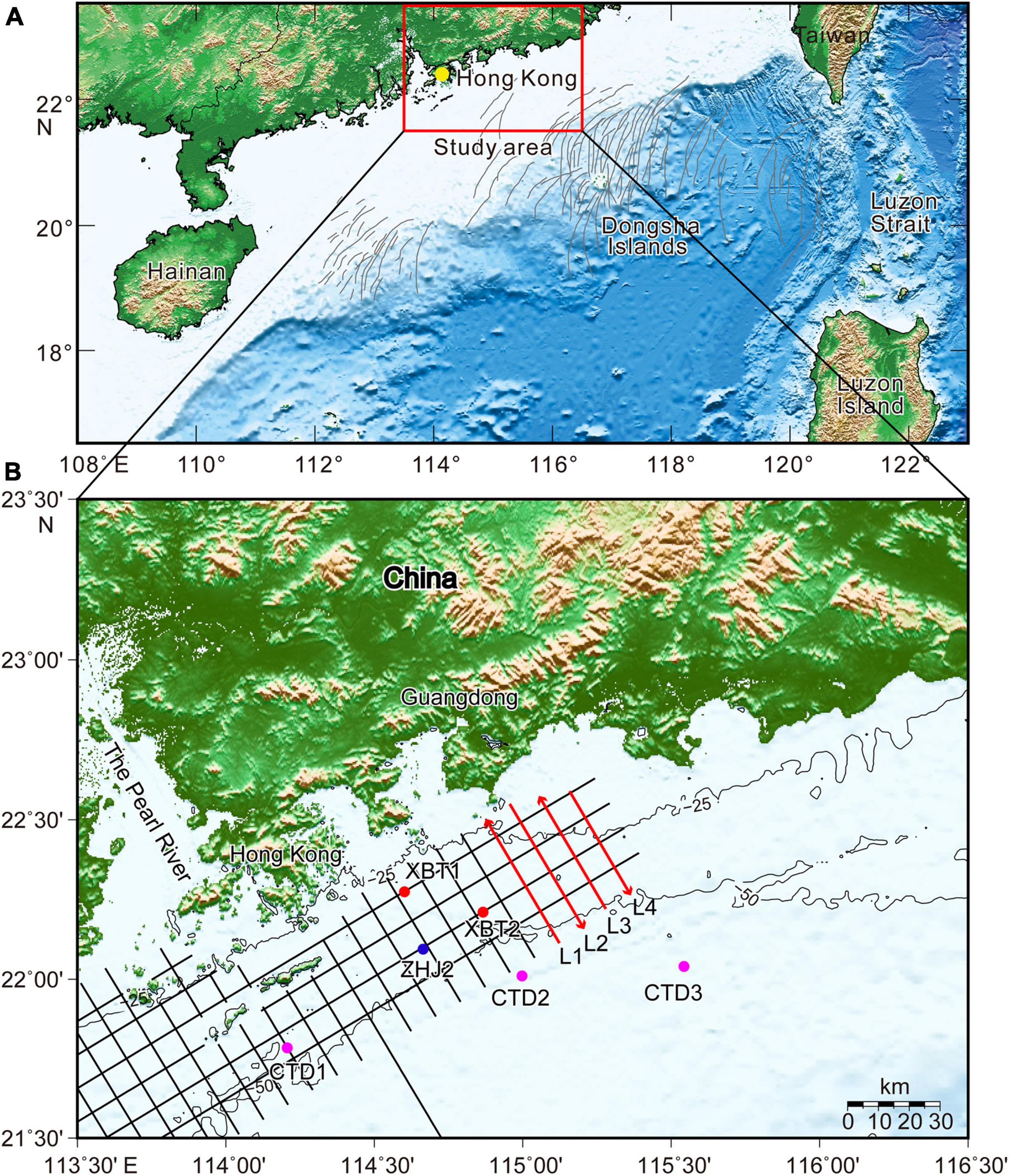
Figure 1. Bathymetry of the northern South China Sea (A) and shallow water offshore of Guangdong (B). Gray curves are the satellite-imaged ISWs modified from Zhao et al. (2004) and Li et al. (2011). The black and red lines denote the acoustic backscatter survey lines acquired in July 2020. The red arrows indicate the directions of the survey lines. The solid circles show the locations of two XBT sites (red), CTD stations (magenta, Chen et al., 2017), and taut-line mooring station ZHJ2 (blue, Lee et al., 2021).

Materials and Methods

Acoustic Backscatter Data Acquisition and Processing

In the shallow water offshore Guangdong Province (Figure 1), approximately 3100 km acoustic backscatter data were collected in July 2020 using an Innomar SES2000 Light parametric sub-bottom profiler, with primary frequency (approximately 100 kHz) and ping rate (up to 50 pings/s). The draft (source depth) of the transducer was 2 m. In this study, we focused on the four easternmost lines with a NW-SE direction (L1–L4; Figures 1, 2) to study the spatiotemporal evolution of the ISWs on the continental shelf. These lines captured a soliton train three times in 20 h repeatedly (Figure 2).

FIGURE 2

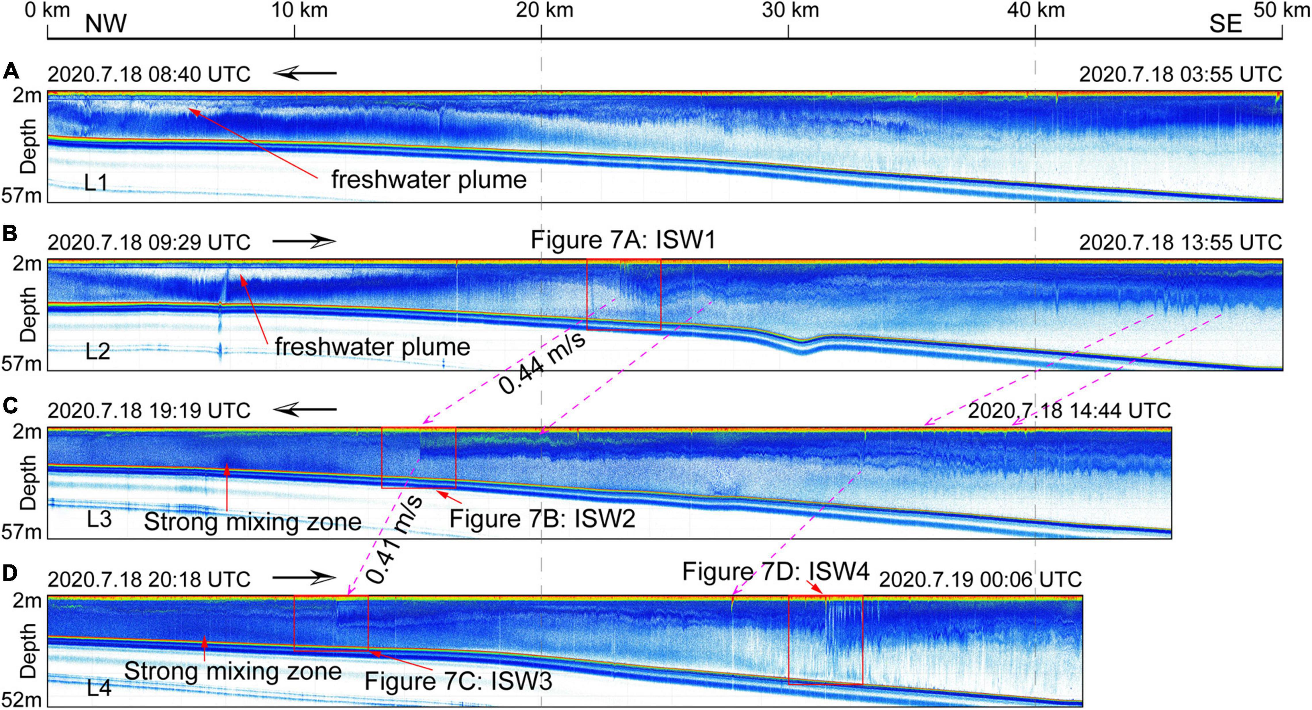
Figure 2. Acoustic backscatter images of ISWs show the fine structure of the water column along the survey lines of L1 (A), L2 (B), L3 (C), and L4 (D) in Figure 1. The survey times and directions are marked by notes and black lines with arrows. Magenta dashed lines with arrows indicate that the same wave crests acquired more than once in different backscatter images, and the mean phase velocities between ISW1, ISW2, and ISW3 are marked. Note that a soliton train (ISW1, ISW2, and ISW3), with apparent vertical and horizontal scales of ∼7 and 100 m, respectively, was captured up to three times within 20 h.

Innomar ISE software (Innomar Technologies GmbH) was used to process the acoustic backscatter data. The acoustic image processing flow was (1) envelope algorithm imaging; (2) noise attenuation by median filter; and (3) time-depth conversion assuming an averaged sound speed of 1500 m/s.

Satellite Imagery

Optical satellite images, such as Moderate Resolution Imaging Spectroradiometer (MODIS) and Visible Infrared Imaging Radiometer Suite (VIIRS) images, are widely used in ISW studies (Li et al., 2013; Tang et al., 2014, 2015, 2018). True color satellite images with a spatial resolution of 250 m are available from the website.¹ In this study, the data from MODIS and VIIRS sensors on NASA spacecraft (Terra, Aqua, NOAA-20, and Suomi) were used to image the sea surface signature induced by ISWs (Figures 3, 4). Benefitting from the good weather conditions on July 18 and 19, 2020, the ISWs in the shallow water region were clearly imaged by three satellite datasets. The mean wave propagation speeds and directions can be measured from the spatiotemporal variations in the satellite images and acoustic backscatter data (Figures 3, 4).

FIGURE 3

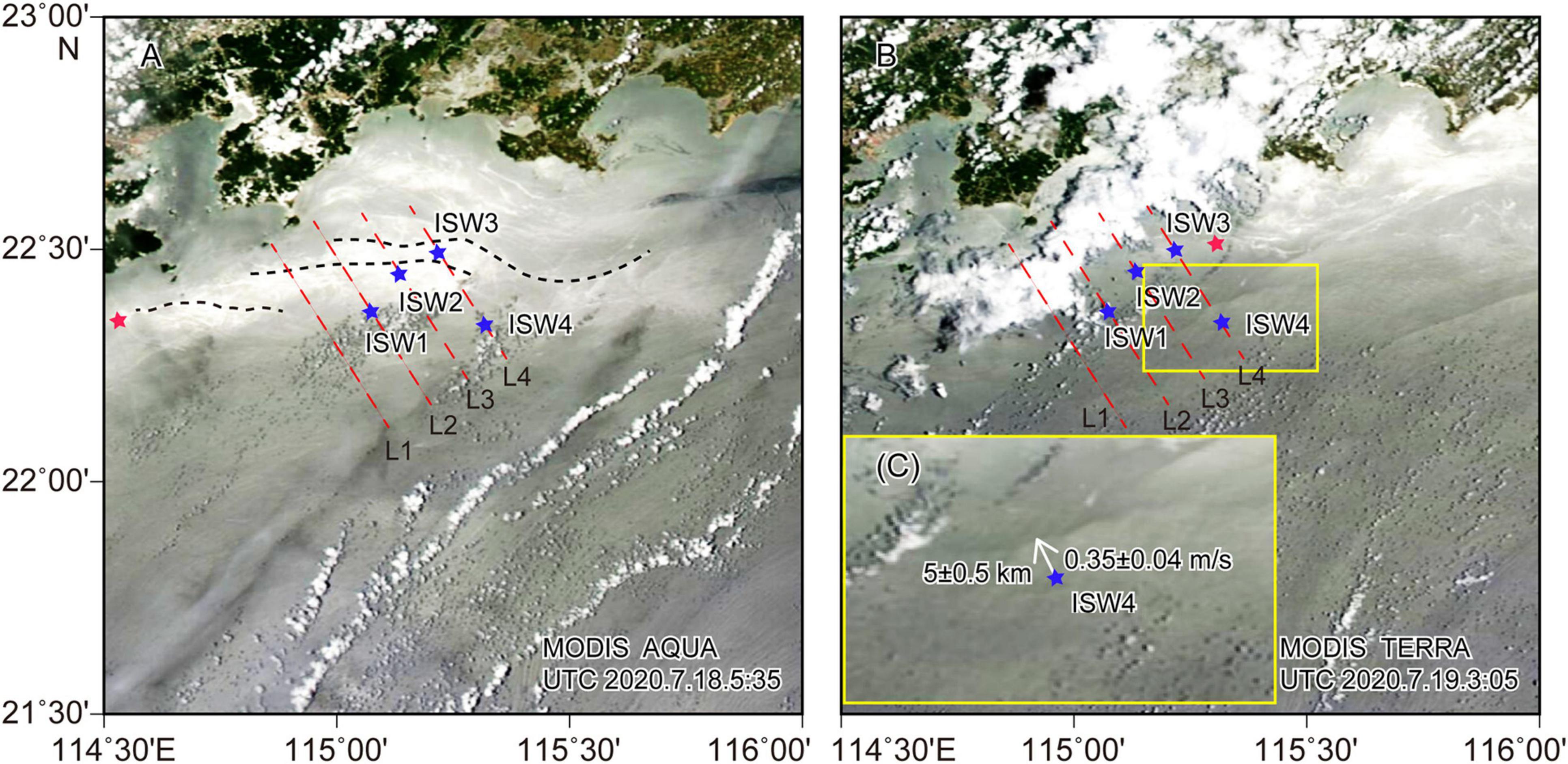
Figure 3. Moderate Resolution Imaging Spectroradiometer images of the ISWs acquired by NASA Aqua (A) and Terra satellites (B) at 05:35 UTC on July 18, 2020 and 03:05 UTC on July 19, 2020. The yellow border illustration (C) is a partial enlargement of panel (B). Red dashed lines are the acoustic backscatter survey lines of L1, L2, L3, and L4, and solid blue pentagrams show ISW positions identified from the backscatter images. The black dashed curves in panel (A) indicate the wave crest of ISWs with large displacement in the study area. Red solid pentagrams indicate the western boundary of the strong ISW dissipation zone, and the distance between the positions of these two pentagrams is approximately 82 km (eastward-moving velocity 1 m/s).

FIGURE 4

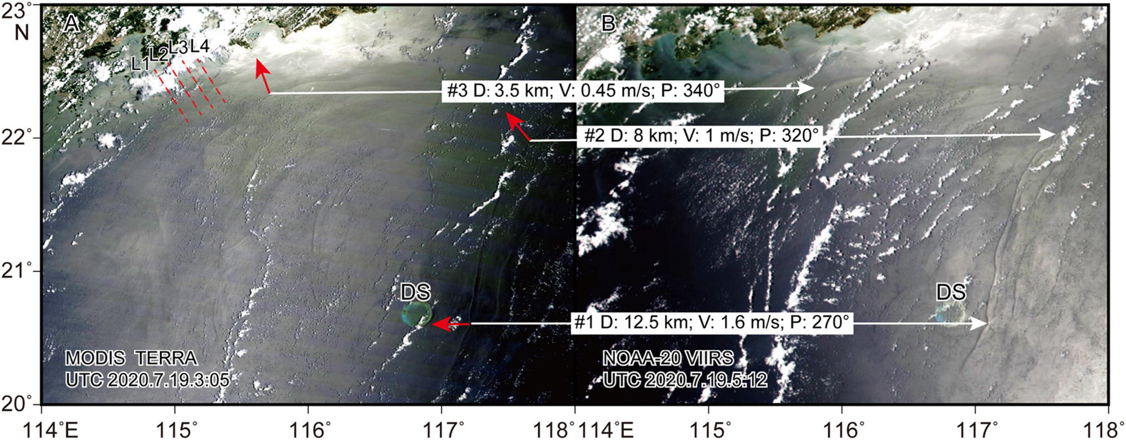
Figure 4. Two satellite images of the ISWs acquired by NASA MODIS Terra (A) and 20 VIIRS satellites (B) with an approximately 2-h lag. Propagation distances, mean velocities, and directions (solid red lines with arrows) were measured between the two images with similar wave crests (white solid lines with arrows). Red dashed lines are the acoustic backscatter survey lines of L1, L2, L3, and L4. D, distance; V, mean speed; P, direction of propagation (clockwise from north); DS, Dongsha Plateau.

Hydrographic Data

During the cruise, two XBTs were deployed simultaneously along the survey lines on July 9th at 13:24 and July 10th at 20:25 UTC (Figures 1, 5). The in situ XBT data, less than 50 km away from the four acoustic backscatter survey lines (L1, L2, L3, and L4), could be used as the background temperature structure in the study area in early summer (Figure 5).

FIGURE 5

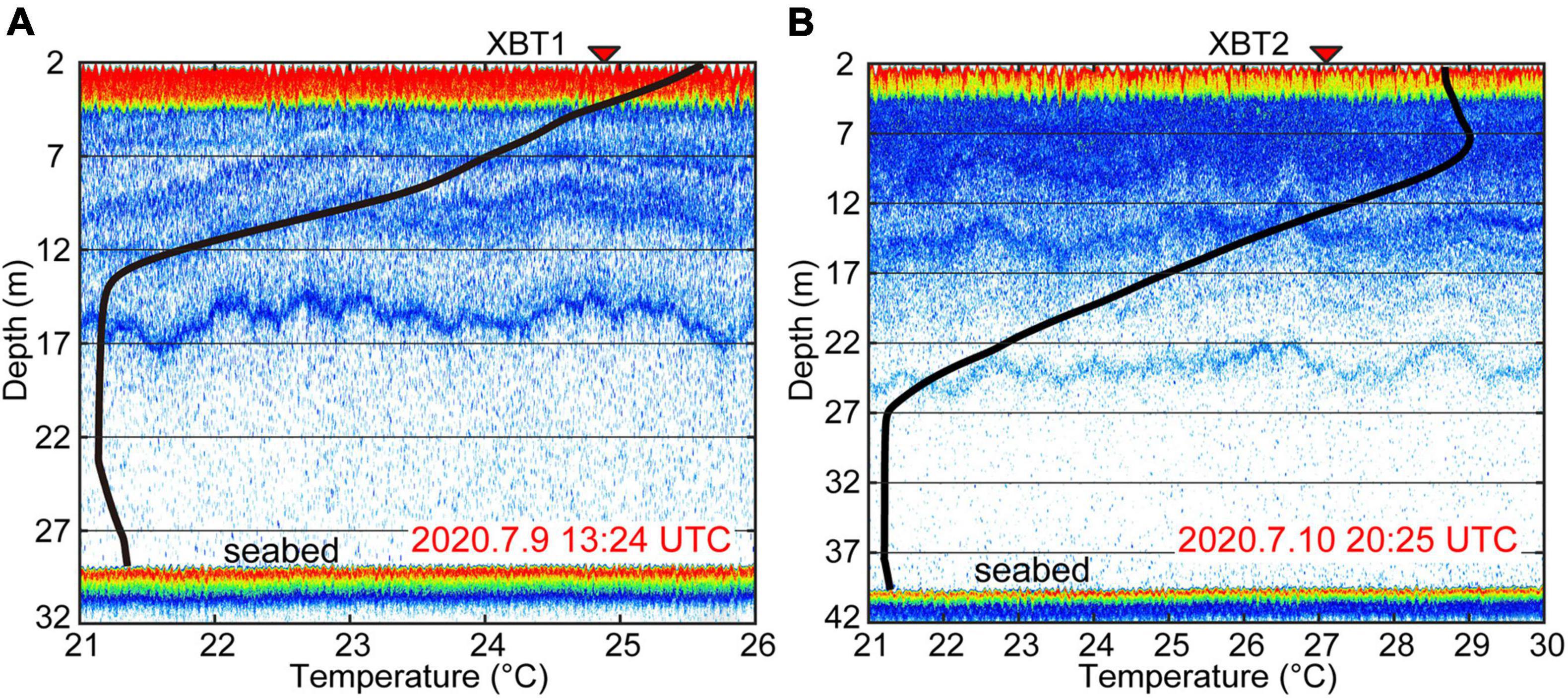
Figure 5. Comparisons of acoustic backscatter images and in situ XBT1 (A) and XBT2 (B) data (black curves) with each other with a small difference of fewer than 3 m, and the red characters indicate the time of acquiring XBT data. Locations of the stations are shown in Figure 1.

Depth profiles of temperature and salinity from three CTD stations were collected from July 27th to August 16th, 2009 (Figures 6A,B; Chen et al., 2017). These historical temperature and salinity data reveal that the water structure can be simplified as a two-layer structure according to the depth of the mixed layer in the study region (Figure 6). Therefore, two-layer structures are finally composited for theoretical KdV and eKdV model calculations and result validation for corresponding ISWs.

FIGURE 6

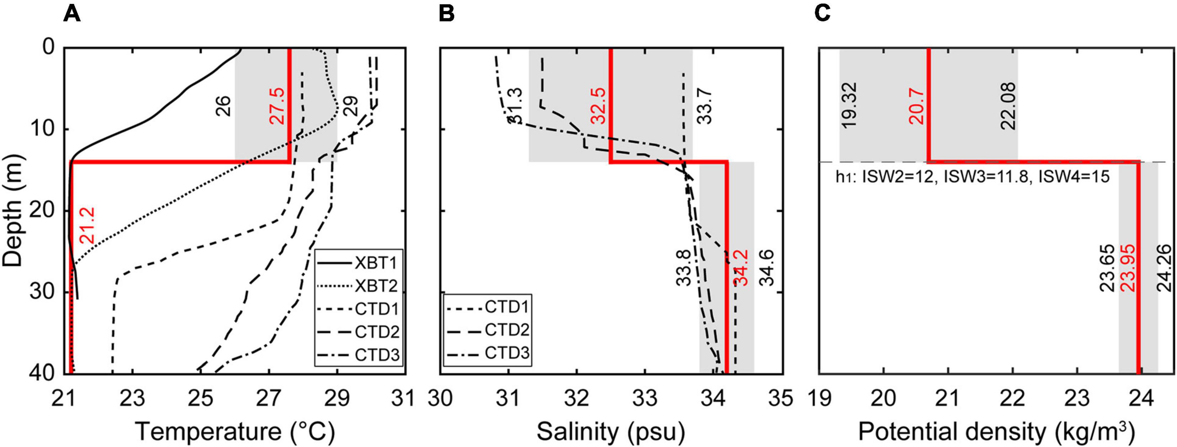
Figure 6. Temperature profiles of the XBT and CTD stations (A) and salinity profiles of the CTD stations (B). The CTD data were collected from July 27 to August 16, 2009 (modified by Chen et al., 2017). The gray filled shades indicate the possible ranges of the temperature (A), salinity (B), and potential density (C) of the upper layer and the lower layer in the study area according to the XBT2, CTD1–3, and ZHJ2 data, and the solid red lines represent the median values of the possible range. The locations of the XBT, CTD, and ZHJ2 stations are shown in Figure 1.

Sea surface temperature (SST) images used in this study were derived from the Group for High Resolution Sea Surface Temperature (GHRSST) data, which are available from the NOAA website.² The daily GHRSST data are satellite-composite products by the Jet Propulsion Laboratory (JPL) with a spatial resolution of 1 km derived from the Advanced Microwave Scanning Radiometer (AMSRE), MODIS, WindSat, Advanced Very High Resolution Radiometer (AVHRR), and in situ observation data.

Theoretical Two-Layer Model of Korteweg-de Vries and Extended KdV Equations

In the continental shelf of this study region (shallower than 300 m), the water column stratification can often be simplified as a two-layer structure according to the density structure (Figure 6). Therefore, we can use a two-layer model to calculate the non-linear phase velocity and the characteristic half-width of ISWs in the study area (Ostrovsky and Stepanyants, 1989). An internal soliton propagation process in continuous water stratification can be described by the KdV equation (Djordjevic and Redekopp, 1978):

$\frac{\partial \eta }{\partial t}+(c+\alpha \eta )\frac{\partial \eta }{\partial x}+\beta \frac{{\partial }^3\eta }{\partial x^3}=0(1)$

and eKdV equation:

$\frac{\partial \eta }{\partial t}+(c+\alpha \eta +{\alpha }_1{\eta }^2)\frac{\partial \eta }{\partial x}+\beta \frac{{\partial }^3\eta }{\partial x^3}=0(2)$

where c, β, α, and α₁ are the linear phase velocity, dispersive coefficient, quadratic, and cubic non-linear parameters, respectively. For the simplified two-layer water stratification model, these parameters can be calculated from the following relationships (Ostrovsky and Stepanyants, 1989):

$c={[\frac{g({\rho }_2-{\rho }_1)h_2{h}_1}{{\rho }_2{h}_1+{\rho }_1{h}_2}]}^{1/2},(3)$

$\beta =\frac{c{h}_1{h}_2}{6}\frac{{\rho }_1{h}_1+{\rho }_2{h}_2}{{\rho }_2{h}_1+{\rho }_1{h}_2},(4)$

$\alpha =\frac{3}{2}\frac{c}{h_1{h}_2}\frac{{\rho }_2{h}_1^2-{\rho }_1{h}_2^2}{{\rho }_2{h}_1+{\rho }_1{h}_2},(5)$

${\alpha }_1=\frac{3c}{{(h_1{h}_2)}^2}[\frac{7}{8}{(\frac{{\rho }_2{h}_1^2-{\rho }_1{h}_2^2}{{\rho }_2{h}_1+{\rho }_1{h}_2})}^2-\frac{{\rho }_2{h}_1^3+{\rho }_1{h}_2^3}{{\rho }_2{h}_1+{\rho }_1{h}_2}],(6)$

where h₁, h₂, ρ₁, and ρ₂ are the thicknesses and the densities for the upper and lower layers, respectively.

For finite-amplitude waves, the theoretical ISW solutions of Equations 1, 2 have the following form (Ostrovsky and Stepanyants, 1989):

$\{\begin{array}{c}\eta ={\eta }_0\text{sec}{h}^2[\frac{x-Vt}{\mathrm{\Delta }}]\hfill \\ V_{K\text{d} V}=\text{c}+\frac{\alpha {\eta }_0}{3}\hfill \\ {\mathrm{\Delta }}^2=\frac{12\beta }{\alpha {\eta }_0}\hfill \end{array}(7)$

$\{\begin{array}{c}\eta =\frac{A}{1+B\text{cos}h(\frac{x-vt}{D})}\hfill \\ B=1+\frac{{\alpha }_1}{\alpha }{\eta }_0\hfill \\ A={\eta }_0(1+B)\hfill \\ V_{\text{eK} dV}=\text{c}+\frac{\alpha A}{6}=V_{KdV}+\frac{{\alpha }_1{\eta }_0^2}{6}\hfill \\ D^2=\frac{6\beta }{\alpha A}\hfill \end{array}(8)$

where Δ, D, V_KdV, and V_eKdV are the characteristic widths and the phase velocities from the KdV and eKdV models, respectively.

Therefore, the vertical velocities of particle motions can be computed from the analytical solutions (7) and (8) via partial derivative W(x) = ∂⁡η(x,t)/∂⁡t|_{t = 0} (Trevorrow, 1998; Teague et al., 2011):

$W(x)=-\frac{2V_{K\text{d} V}{\eta }_0}{\mathrm{\Delta }}\text{sec}{h}^2(x)\tanh (x)(9)$

and

$W(x)=\frac{B{V}_{\text{e} KdV}}{AD}{\eta }^2(\frac{x}{D})\sinh (\frac{x}{D})(10)$

for the KdV and eKdV models, respectively.

Results

Characteristics of Internal Solitary Wave Packets

Many ISW packets were captured during the survey cruise using 100-kHz acoustic backscatter data in early summer 2020 (Figure 2). Due to continuous and repeated observations of the ISWs, some soliton trains were captured more than once, as shown with similar features and reasonable locations on different lines. In this study, four representative wave packets (ISW1, ISW2, ISW3, and ISW4) at water depths from 24.5 to 40 m were selected for further analysis (Figure 2). Figure 7 shows the detailed backscatter feature and the strategy of deriving the waveform parameters for ISW1, ISW2, ISW3, and ISW4. The captured locations for each leading soliton are plotted in Figure 3, while the observed parameters of positions, times, upper layer thicknesses, water depths, amplitudes, and full widths of these ISWs are listed in Table 1.

FIGURE 7

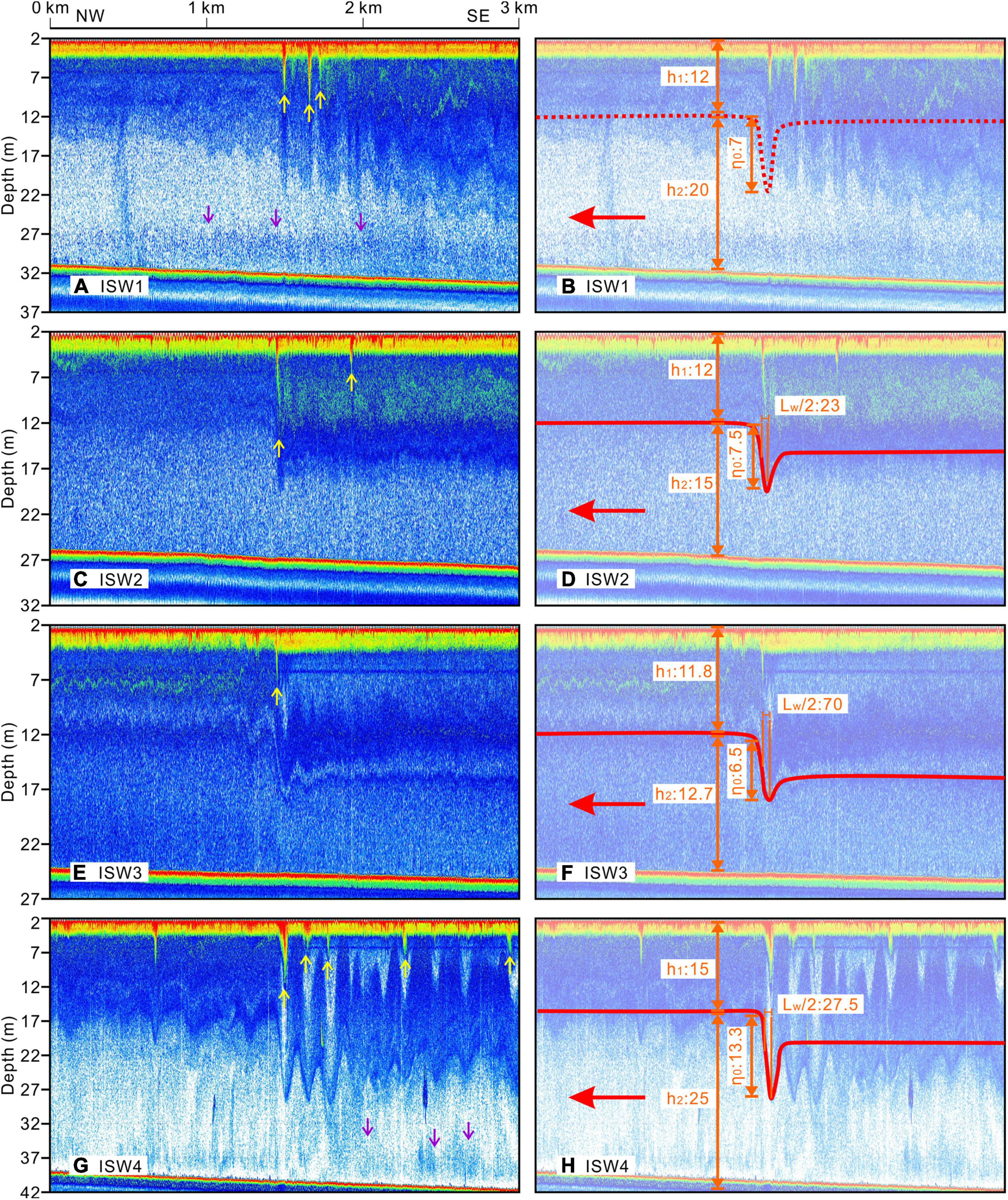
Figure 7. Acoustic backscatter images show the waveforms (left) of ISW1 (A), ISW2 (C), ISW3 (E), and ISW4 (G). The red lines and orange notes (right) are used to derive the waveform parameters of ISW1 (B), ISW2 (D), ISW3 (F), and ISW4 (H). The red, yellow, and purple arrows represent the propagation directions of these ISWs, the ISW-induced bubble plumes, and sediment resuspension, respectively.

TABLE 1

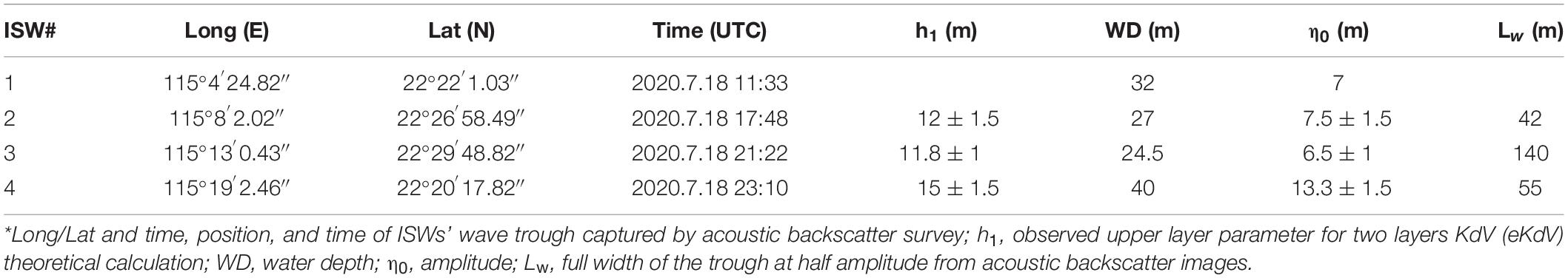
Table 1. Observed parameters of the ISWs*.

ISW1, ISW2, and ISW3 are from the same soliton train captured three times within 20 h from west to east on the repeating acoustic sections of L2–L4 (Figures 2, 7). ISWs propagated from deeper water (32 m) to the shoaling water (24.5 m) from approximately south to north (Figures 2, 7A–F and Table 1). The wave packet ISW1 was first captured on the L2 section, as it had no appearance on the preceding section L1 (Figure 2). The packet consists of at least four solitons with positive polarity and representative waveforms within the first 0.5 km from the leading soliton (Figure 7A). The solitons’ amplitudes are not ordered from the leading soliton to the trailing ones. The third soliton has the largest amplitude of 9 m, while the leading wave amplitude is approximately 7 m. Approximately 0.5 km behind the leading soliton, wave fields become chaos, and solitons are not easy to identify. The passing packet deepens the mixed layer, forming a bore-like structure of ∼2 km. At the trough of the bore, the thickened mixed layer induced by the passing ISWs reverses the non-linear parameter α, and thus, elevated waves are formed (Figure 2B).

In contrast, packets ISW2 and ISW3 only have one leading soliton individually (Figures 2C,D, 7C–F). Similar to ISW1, the amplitudes of the leading waves of ISW2 and ISW3 are ∼7 m, but their following wave amplitudes are only 1–2 m and cannot be recognized as solitons. The mixed layer is suppressed to specific depths after passing the solitons, forming hydraulic jumps. Therefore, the solitons only have leading edges, and rear edges are not well developed, indicating a significant energy loss, and the stratifications are failed to be restored to the starting depths within ∼10 km (Figures 2C,D).

On line L4 in the deeper water region, the large soliton train (ISW4) with more than 10 following well-developed solitons was captured 2 h beyond ISW3 and ∼20 km away from ISW3 (Figures 2D, 7G). The soliton amplitudes of ISW4 are sequentially ordered from the leading wave (∼13.3 m) to the trailing waves (∼5 m). In addition to the deepened mixed layer, the sediments were suspended several meters above the seafloor after passing the solitons (Figure 7G). Meanwhile, because of its larger spatial scale, ISW4 can be observed from the satellite image (Figures 3B,C).

From two satellite images acquired by NASA MODIS Terra and NOAA-20 VIIRS satellites on July 19th, 2020 (1 day after acoustic backscatter survey), many alternating dark and light curving signatures were caused by ISWs from the Dongsha Plateau to the Guangdong coastal water (Figure 4). The propagation speeds and directions vary significantly from the deep-water region to the shallow water region according to the position differences of the ISW crests with a 2-h lag (Figure 4). The propagation speeds at locations #1–#3 gradually decrease from ∼1.6 to 0.45 m/s, and the propagation directions turn from ∼270° to 340°, corresponding to the shoaling water depth from the continental shelf to the coastal area. Therefore, it is expected that the ISWs observed from the acoustic images in the study region should have propagation parameters similar to those of the satellite-observed results at location #3 (Figure 4).

By identifying the time and space differences of the wave crests using the backscatter data, the estimated mean propagation velocities were ∼0.44 m/s (between ISW1 and ISW2) to ∼0.41 m/s (between ISW2 and ISW3), assuming that the ISWs were propagating northward (Figure 2). However, the propagation velocities of ISW1, ISW2, and ISW3 cannot be determined by satellites because of their small spatial scales. Therefore, we resort to the theoretical calculation to verify the propagation in the next section. In contrast, ISW4 on L4 was captured by the MODIS image ∼4 h after capture by acoustic backscatter observation (Figure 3C). The estimated mean propagation velocity of ISW4 from the acoustic backscatter to the satellite is ∼0.35 ± 0.04 m/s, which is less than the results from two satellite images in the coastal region (Figure 4).

Characteristics of the Internal Solitary Wave Packet From Theoretical Calculations

Water Properties and the Simplified Two-Layer Model

In situ XBT data show that the temperature of the upper mixed layer gradually decreases from the near-surface to the lower layers (XBT1: 26.2–21.2°C; XBT2: 29–21.2°C; Figure 5). In contrast, the lower layer temperature is nearly homogeneous with a small temperature variation (21.14–21.38°C). The acoustic backscatter images show multiple strong scattering layers in the upper mixed layer, corresponding well to the strong temperature stratification. The scattering feature in the lower layer is substantially weak without a continuous scattering interface. The overall water column stratification revealed by acoustic backscatter data (XBT1: 15 m; XBT2: 24 m) and XBT profiles (XBT1: 14 m; XBT2: 27 m) is consistent with a small vertical difference of less than 3 m, indicating that the acoustic backscatter technique is suitable for imaging the water structure. Therefore, the thicknesses of the upper and lower layers were derived from acoustic backscatter data (Figure 7 and Table 1).

For the simplified two-layer model, which is used to estimate the theoretical parameters for the ISWs, proper temperature and salinity values must be calculated for each layer. The model temperature is straightforwardly derived from in situ XBT2 because XBT2 is closer to the study region and fits well to the historical CTD data (Figure 6A). Therefore, the upper layer is assigned 27.5°C, and the lower layer is assigned 21.2°C (Figure 6A). Meanwhile, according to the salinity data of the CTD stations, as well as the ZHJ2 station (Figure 6B), the salinity values of the upper and lower layers are assigned to be 32.5 and 34.2 psu, respectively (Figure 6B). Thus, the density models can be estimated using the equation of state of seawater (Figure 6C; Millero et al., 1980; Fofonoff and Millard, 1983).

Propagation Velocities From the Model Prediction

A proper ISW propagation model can be used to predict the ISW speed, which should be comparable to the values from satellite and acoustic methods (e.g., Tang et al., 2015). Here, phase velocities are derived from two-layer KdV and eKdV models with varying salinity (Figure 6) for ISW packets: 0.48/0.41 (ISW2), 0.44/0.38 (ISW3), and 0.63/0.5 m/s (ISW4) (Figure 8). The results show that the salinity variation in the range of 31 to 34 psu in the upper layer can significantly affect the phase speed. We can see that the KdV model predicted values of ISW2 and ISW3 are slightly larger than the propagation velocities estimated from the acoustic backscatter data, while the eKdV model predicted values are slightly smaller than the estimated propagation velocities. The analytical result of ISW4 (0.63/0.5 m/s) is larger than the acoustic satellite measured velocity (0.35 m/s). The two-layer eKdV model result of ISW4 returns much better agreement with the observations than the KdV model result. A lower salinity value in the two-layer model, the uncertainty of layer thickness, and the spatial resolution of the satellite images may be error sources for both predicted and measured propagation speeds.

FIGURE 8

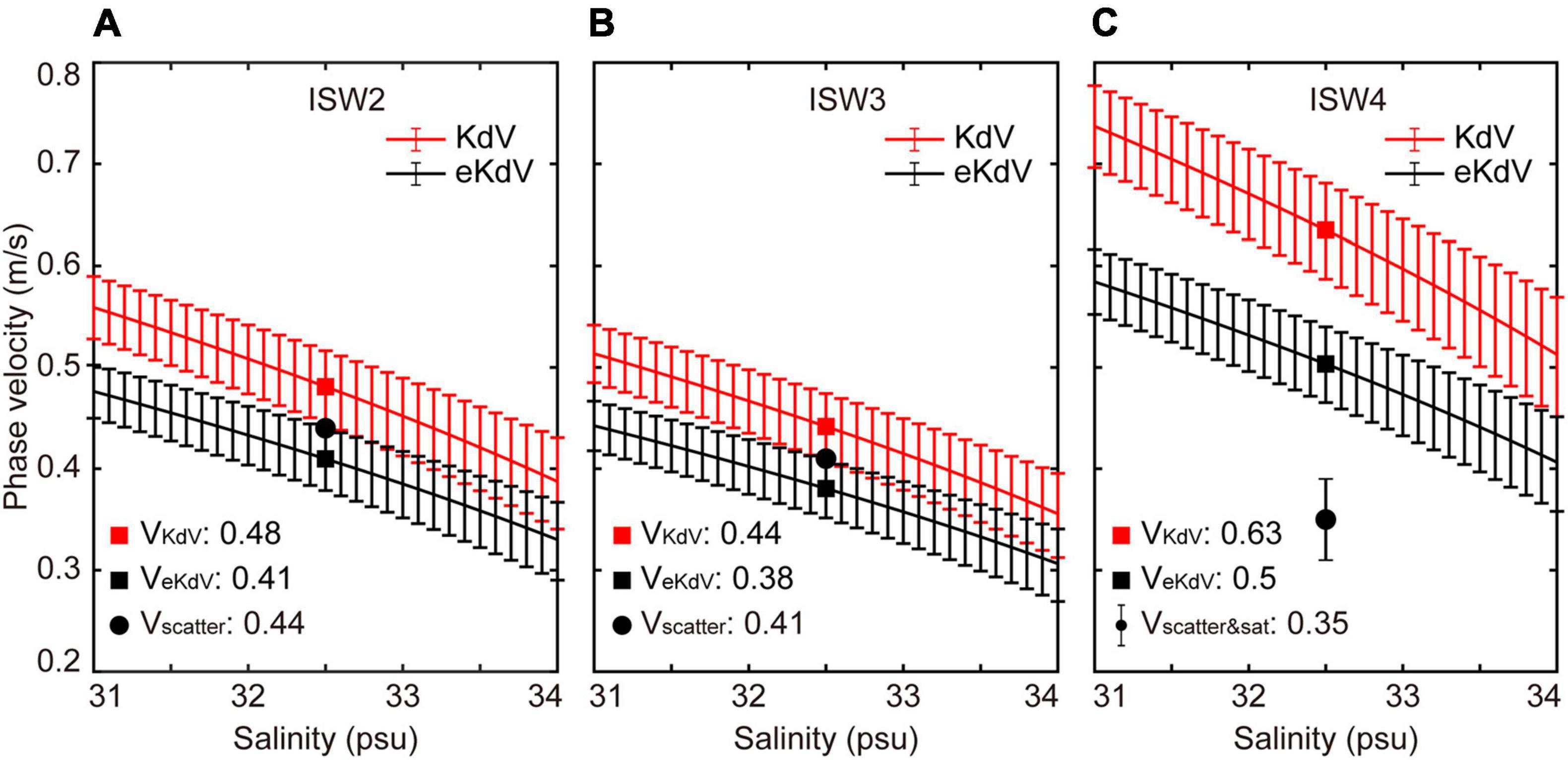
Figure 8. Phase velocities of ISW2 (A), ISW3 (B), and ISW4 (C) derived from the two-layer KdV (red) and eKdV (black) models with different salinity parameters of the upper layers (curves with error bars). The solid squares represent phase velocities calculated using the median densities of two layers shown in Figure 6C. The solid black circles and solid black circle with error bar indicate the phase velocities of the ISW packets derived from acoustic backscatter data and satellite and acoustic backscatter data, respectively.

Waveforms

Using Equations 7, 8, the analytical waveforms and the characteristic widths for the ISWs are calculated (Figure 9). The analytical waveforms overall patterns of the KdV and eKdV models are similar. However, the detailed features of the observed and theoretical waveforms are quite different. For example, analytical waveforms are in perfect symmetry, while the observed waveforms are in typical asymmetry with distinct differences between the leading edge and the rear edge.

FIGURE 9

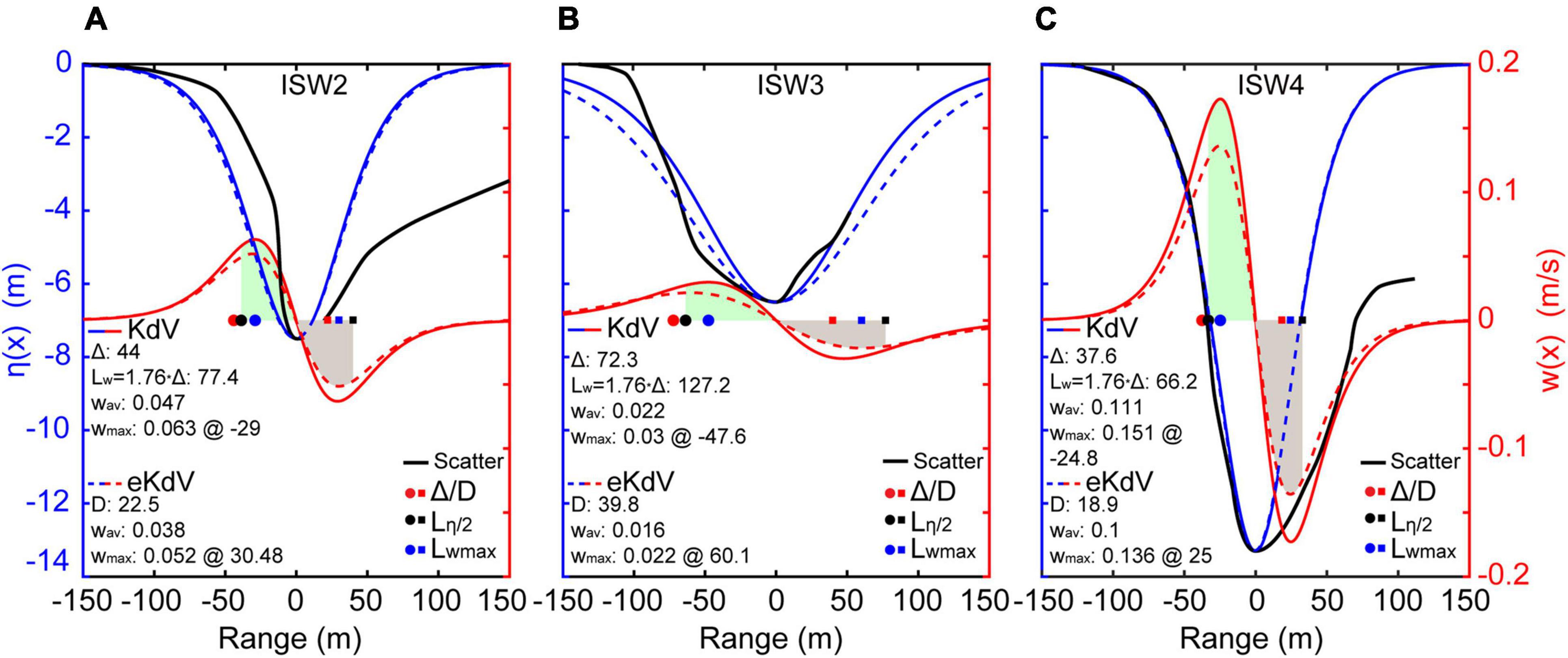
Figure 9. Double-axis plots of the predicted waveforms (blue) and vertical velocities (red) using the two-layer KdV (solid curves) and eKdV (dashed curves) model for ISW2 (A), ISW3 (B), and ISW4 (C). Three solid dots and squares are the characteristic width Δ/D (red), half-width L_η/2 = L/2 (black), and maximum vertical velocity point L_wmax (blue). The filled shades are for integrating the mean vertical velocity of the two-layer KdV (green) and eKdV (gray) model between the half-width point and the trough. Black lines are the waveforms derived from backscatter data. Δ/D, characteristic width; L_w, half-wave width; W_av, mean vertical velocity; W_max, maximum vertical velocity.

Since the wavelengths L_w are derived from the analytical ratio of 1.76 between the wavelength parameter L_w and the characteristic width Δ of the KdV model (Tang et al., 2014, 2015). The waveform parameters of wavelengths of ISW2, ISW3, and ISW4 are compared from the analytical and acoustical results (Table 1 and Figure 9), as wavelength of ISW1 cannot be obtained from the backscatter data (Figure 7A). The L_w values of ISW2 and ISW3 measured directly from the acoustic backscatter data are ∼42 and ∼140 m, respectively. The angle theta between the near-northward wave propagation and the backscatter observation line may make the imaged apparent wavelength wider by a factor of cos^–1 (30°). In addition, the Doppler effect for the same/opposite moving directions of the ship and wave stretches/shortens the observed wavelength by a factor of V₁/(V₁ − V₂) or V₁/(V₁+V₂), where V₁ and V₂ are the ship and the ISW velocity, respectively. Therefore, the actual wavelengths are ∼32 and ∼136 m by considering the overall contribution between these two effects. The ISW2 wavelength measured from the observed result is half of the analytical result, while the ISW3 observed result matches the analytical result of 127.2 m. For ISW2, the low ratio of 0.8 is probably underestimated since we used the leading edge to estimate the length.

As the survey line is nearly perpendicular to the wave crest (Figure 3B), the leading soliton L_w of ISW4 is 67.6 or 62 m after removing the Doppler effect. The KdV prediction wavelength of 66.2 m is very close to the observed result.

Vertical Particle Motion

Studies have shown that vertical velocities can be measured from acoustically imaged waveforms and predicted from the KdV and eKdV models (e.g., Tang et al., 2015). Vertical particle motion along the waveforms of ISW2, ISW3, and ISW4 can be expressed by Equations 9, 10 (Figure 9). In particular, the maximum velocities and mean velocities (W_av, averaged from the half-width point to the trough of the leading edges, shaded zones) of these three ISWs are also derived (Figure 9). The W_max values from the KdV and eKdV models for ISW2, ISW3, and ISW4 are 6.3/5.2, 3/2.2, and 15.1/13.6 cm/s, respectively, while the mean vertical velocities are 4.7/3.8, 2.2/1.6, and 11.1/10 cm/s, respectively. The vertical velocity ISW2 is nearly twice that of ISW3 from the same packet. The W_max and W_av of ISW4 at a depth of 40 m are nearly twice those of foregoing packet ISW2 at a depth of 27 m.

Other Phenomena Related to Internal Solitary Waves

Internal Solitary Wave-Induced Sediment Resuspension

Strong ISW-induced currents scour the seafloor periodically and successively by shaping the seafloor morphology, suspending the seabed sediments, and controlling the grain size of the regional sediments (Ma et al., 2016; Tian et al., 2019a,b, 2021). The phenomena of sediment resuspension can be easily observed from high-resolution acoustic backscatter data (Cacchione et al., 2002; Reeder et al., 2011; Masunaga et al., 2015; Tian et al., 2019a). In this study, patches of weak scattering intensity (purple arrows) are often observed in the near-bottom layers after passing the ISWs (Figures 7A,G), showing the sediment resuspension process induced by the ISWs. Sediment resuspension is larger than 5 m height above the seafloor, and affects over tens of kilometers. This phenomena, which called bottom nepheloid layer (BNL), is widely recognized in the global ocean (Masunaga et al., 2017; Tian et al., 2019a).

Internal Solitary Wave-Induced Bubble Plumes

Near the sea surface, there is always an extremely strong acoustic scattering layer of a few meters on the acoustic backscatter data (yellow layer; Figures 2, 7). They are caused by bubbles in the near-surface water (e.g., Trevorrow, 2003). The occurrence of a soliton enhances the bubbles and carries the near-surface bubbles into the soliton core, forming a downwelling bubble plume (yellow arrows; Figure 7). Previous studies have shown that these ISW-induced bubble plumes have a bubble size distribution and concentration similar to those of bubble plumes caused by breaking surface waves, which generally begin to appear with wind speeds over 2.5 m/s (e.g., Trevorrow, 1998).

In this study, the plume penetration depths and width induced by ISW1–4 ranged from 8 to 12 and 30 to 70 m, respectively (Figure 7). The penetration depths are controlled by the amplitude of the solitons or the isopycnal of the surface layer. Taking ISW4 as an example, the largest bubble plume with penetration depth (12 m) and width (70 m) is above the core of the leading soliton, and the relatively small bubble plumes with penetration depth (∼7 m) and width (∼20–70 m) correspond to the following small solitons. Such downwelling process forces influence near-surface physical and biogeochemical cycles.

Discussion

Origins of Internal Solitary Waves on the Continental Shelf

There are generally two generation sources of ISWs observed on the continental shelf of the northern SCS. One is remotely from the Luzon Strait, and the other is locally from the northern SCS continental shelf (Lien et al., 2005; Cai et al., 2012). According to satellite images, most ISWs in the northern SCS propagate westward from the Luzon Strait and are refracted near the Dongsha Plateau and then torn by the island into two new trains (northern and southern arms) continuing to propagate northwestward to coastal areas (Li et al., 2013; Wang et al., 2013; Ma et al., 2016).

In this study, we suggest that large-scale ISWs were also generated in the Luzon Strait based on the following considerations. Two satellite images within the acoustic backscatter observation period directly show that large-amplitude ISWs are successively distributed from the Dongsha Plateau to the coastal areas (Figure 4). Meanwhile, ISWs at the Dongsha Plateau must be generated in the Luzon Strait, and ISWs are still traceable tens of kilometers south of the study region evolved from the northern arm of the ISW train (Figure 4). Moreover, the surface signature of ISW4 was clear enough and was captured by both satellite and acoustic backscatter data. Therefore, it can be safely inferred that the periodically active ISWs in the coastal region are generated at the Luzon Strait and then propagate into the study region after long-range evolution.

The acoustic backscatter data may have captured some locally generated internal waves with internal tides on the continental shelf. For example, there is an isolated ISW approximately 1 km ahead of ISW4 in Figure 7G. This ISW does not belong to either the trailing soliton of ISW3 or the leading soliton of ISW4, which are successive ISW packets from the Luzon Strait. Therefore, the isolated ISW might be generated locally with steep topography, most likely at the continental shelf break by the internal tide. More integrated observations are necessary to identify the origins of these ISWs.

Evolution of Internal Solitary Waves on the Continental Shelf

In this study, all ISWs have large amplitude frontal edges and small amplitude rear edges (Figure 7). The frontal edges are steep and well-developed. In contrast, the rear edges are much weaker and fail to resort to the normal depth. It is suggested that these divergent zones of the rear edges were under collapse by losing potential energy and finally forming asymmetric waveforms. The breaking event of ISWs is mostly caused by Kelvin–Helmholtz instability and convective overturn in the steep rear edge, forming the breaking tail of the ISWs. These features are similar to previous simulated and observed results in shelf-coastal regions (Ostrovsky and Stepanyants, 1989; Novotryasov et al., 2015).

Dissipation of Internal Waves in the Coastal Area

Numerical simulations suggest that large internal waves always dissipate energy by developing a dispersive wave tail on gentle slopes (e.g., Vlasenko and Hutter, 2002). The coastal topography in the study region is gentle (slope angle γ < 0.17°) with small variation, and seawater stratification might be a key factor affecting the propagation and dissipation of ISWs. Following the ISW breaking criterion h_b = h₁ + η₀/(0.8°/γ + 0.4), where h_b is the critical water depth for solitary wave breaking (Vlasenko and Hutter, 2002), and according to the stratification parameters of ISW1–4 (Table 1), the critical water depth h_b is approximately 17.5 m. Such a water depth is typically smaller than the water depth (∼30 m) of the study. Therefore, the prediction suggests that stratification favors passing ISWs through the study area with a large leading wave and dispersive trailing waves, consistent with acoustic observations (Figure 7). The trailing waves weaken as the ISWs propagate toward coastal water.

Strong dissipation zones could be identified as a series of bright (white) bands in the northern part of the study region (Figures 3, 4). However, these dissipation zones should differ from the ISW-induced dissipation zones, although they highly overlap with the ISW field spatially. First, there are no clear frontal lines relating to the leading waves of the ISWs. Second, the dissipation zones move eastward with a very high speed, contradicting the northwestward propagating ISWs with quite low speeds.

The water masses in the coastal region are complex. They include solar-heated SCS water in the south, eastward drifting river water, along coastal wind-driven currents, and coastal upwelling cold water. On L1 and L2 in the shallow water region, the acoustic backscatter images show the upper layers with substantially weak without a continuous scattering interface are above the lower thick strong scattering layers (Figure 2). We suggest that these phenomena were the river plumes sitting on top of the seawater close to the river mouth side. Moreover, the SST acquired on July 18 and 19, 2020 in the northern SCS reveals high-temperature SCS water in the south, low temperature close to the shore region, and a transition zone between (Figure 10).

FIGURE 10

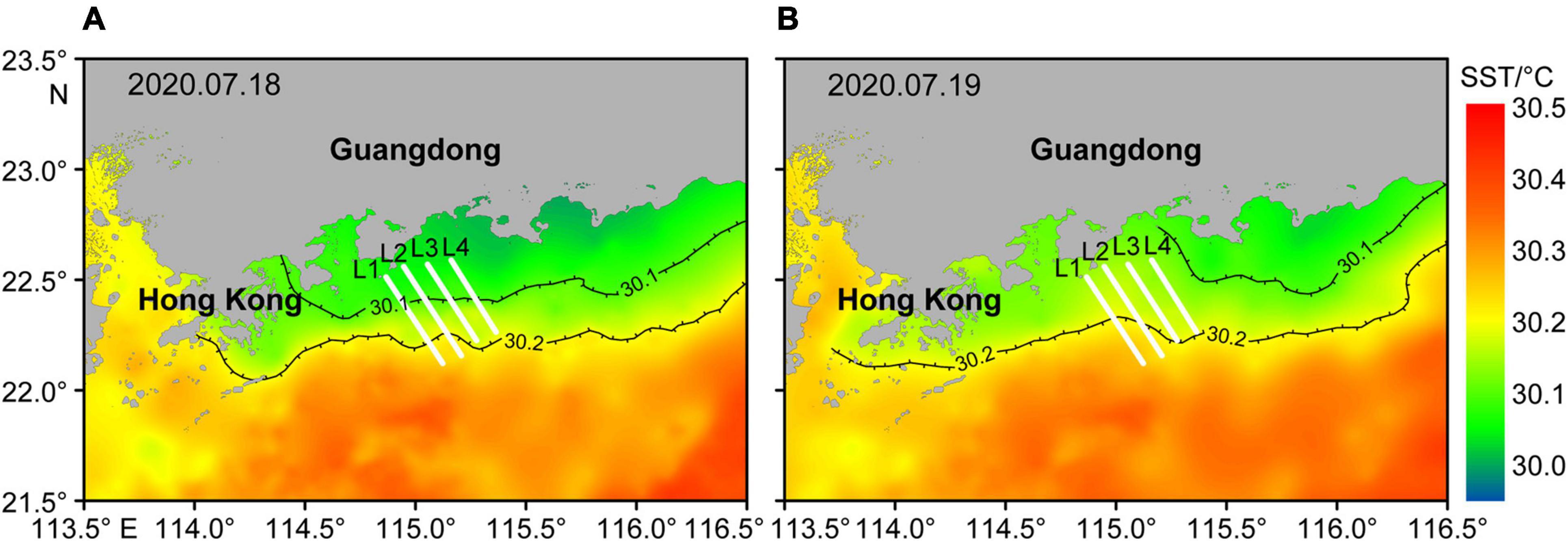
Figure 10. The satellite-composite sea surface temperature (SST) on July 18, 2020 (A) and July 19, 2020 (B) indicates that the study area was influenced by coastal cold water upwelling. The black lines with half ticks represent the transition zone (30.1°C < SST < 30.2°C) and upwelling zone (SST < 30.1°C). The white lines denote the acoustic backscatter survey lines.

The dissipation zones are highly correlated with the temperature transition zone or the frontal zone between the northern ventilated water and southern heated water (Figures 3, 10, 11). On the L3 and L4 acoustic backscatter sections, the scattering feature has been intensified even before the arrival of ISWs (Figure 2). This region is within the dissipation zone on the satellite images and the temperature transition zone on the SST image (Figures 3, 10, 11). Therefore, a schematic model is proposed for internal wave propagation and dissipation in this study region (Figure 12). Far field ISWs generated at the Luzon Strait can penetrate into the wide shelf region because of the strong stratification caused by solar-headed surface water. Distinct dissipation processes at the trailing waves of the ISW packets make the ISWs weaken toward the shoreward region. These ISWs finally disappear before entering the upwelling cold water, as their stratification does not support ISW transmission. The surface dissipation patches are near-surface internal wave breaks induced by the wind force. Their occurrences show a quick response to the wind force along the frontal instability zone.

FIGURE 11

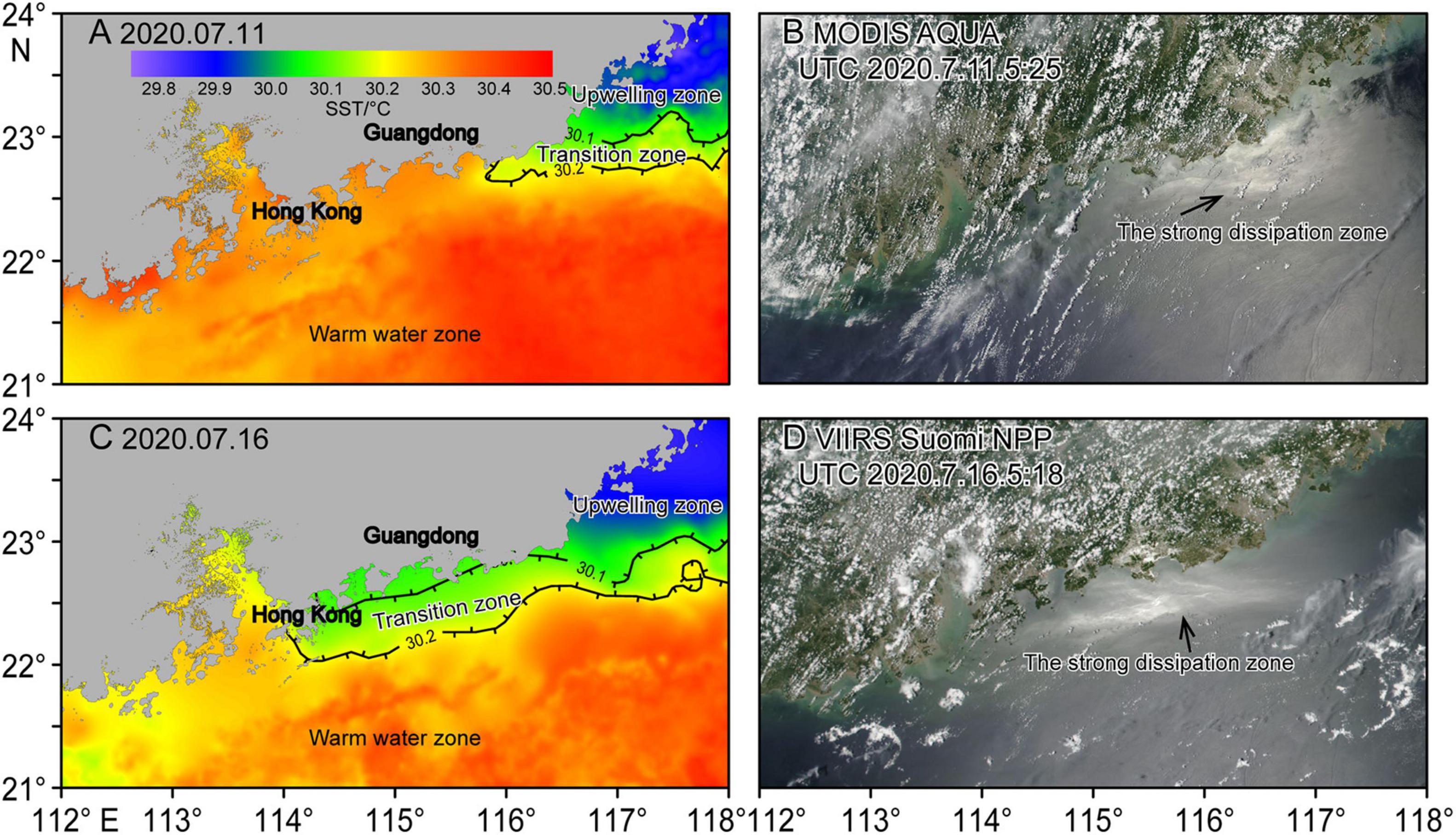
Figure 11. The satellite-composite sea surface temperature (SST) in the study area on July 11, 2020 (A) and July 16, 2020 (C). Satellite images of the surface roughness acquired by MODIS Aqua and VIIRS Suomi NPP at 05:25 UTC on July 11, 2020 (B) and 05:18 UTC on July 16, 2020 (D). Comparisons of SST images and satellite images on the same day show that the strong ISW dissipation zones (white wave crests) coincided with the transition zone of the upwelling region (30.1°C < SST < 30.2°C).

FIGURE 12

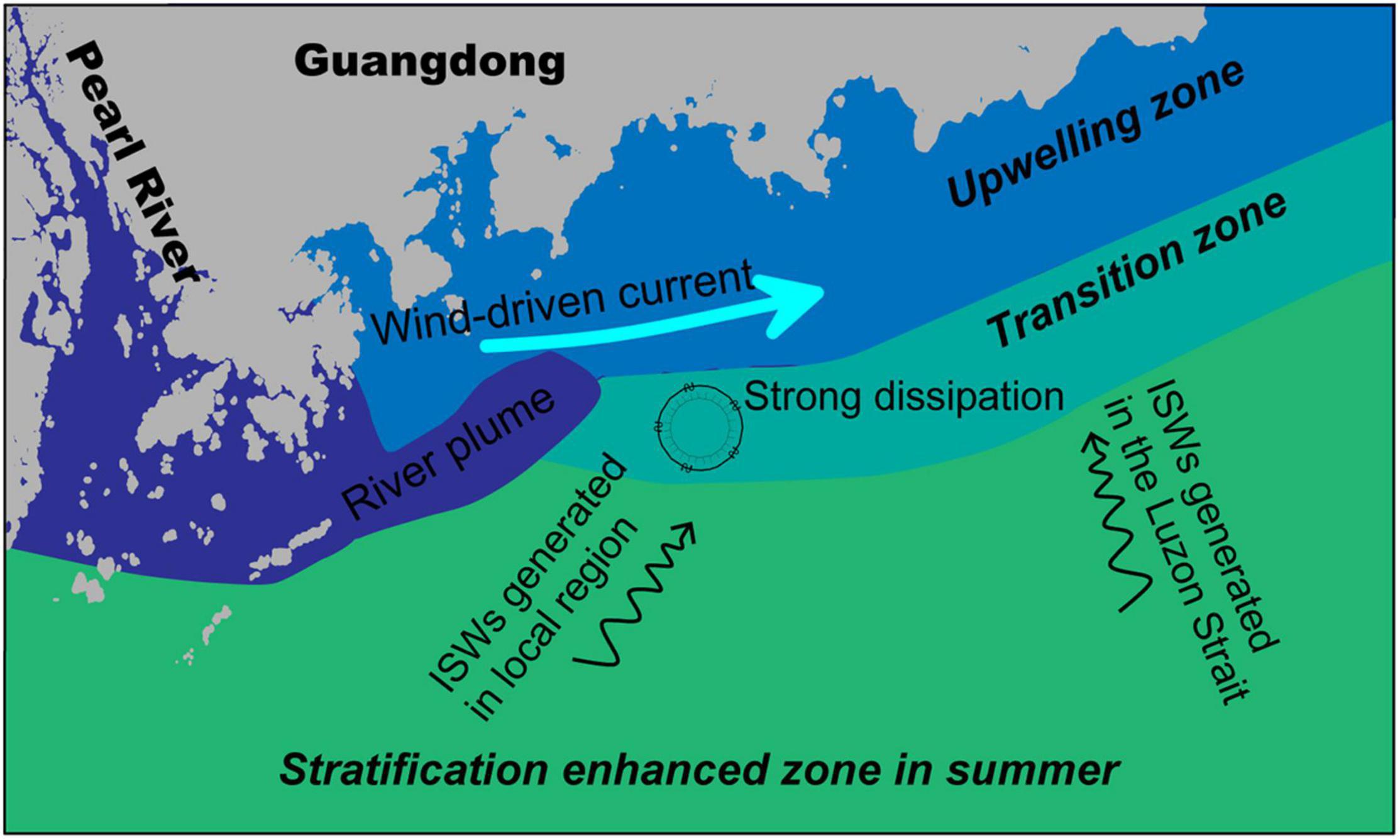
Figure 12. Schematic diagram describing the propagation and dissipation processes of the ISWs. The ISWs on the continental shelf of the northern SCS are generated in the Luzon Strait and northern SCS shelf. The dissipation and evolution of ISWs couple multiple mechanisms among river plume dispersal, upwelling mixing, and wind-driven currents.

Offshore Engineering Implications

Our study area is offshore of the Guangdong–Hong Kong–Macao Greater Bay Area. It is one of the most developed areas in China. There are numerous near-shore artificial facilities in the study area, such as wind power facilities, cross-sea bridges, oil platforms, and submarine cables. Large amplitude ISWs can lead to strong horizontal and vertical currents in the ocean. A few studies have been carried out to evaluate the impact induced by strong waves on offshore structures (e.g., Cai et al., 2006). This study shows that the duration of ISWs is a few minutes, and the vertical displacements and vertical velocities are on the order of ∼10 m and 10 cm/s, respectively. For example, ISWs recorded that the vertical displacement was up to 20 m at a period of ∼6–8 h at station ZHJ2 (Figure 1; Lee et al., 2021).

During the cruise, a high-resolution multichannel streamer, which is geophysical equipment used in near-surface engineering surveys, was deployed simultaneously with acoustic backscatter. Due to the lack of depth controlling units, the streamer went through strong vertical movements induced by ISWs, resulting in apparent undulating topography waves of ∼500 m wavelength and ∼2–4 m amplitude. Tang et al. (2015) have also reported that the streamer with depth controlling units was uplifted to the surface by the ISWs for ∼20 min (∼3 km) in NE SCS. In addition, offshore engineering vessel operations, such as dynamic positioning and drilling, are often influenced by ISWs.

Artificial facility safety is sensitive to sediment siltation or erosion on the seafloor. ISWs can give rise to remarkable interactions between the seafloor and ocean currents in a relatively short time (Apel et al., 2007; Huang et al., 2016). The total amount of sediments resuspended by the ISWs is 2.7 times that of the sediments supplied by the river in the northern SCS (Jia et al., 2019). The suspended sediments diffuse along the isopycnals and redeposit in a different area depending on sediment grain sizes and ocean currents (Tian et al., 2019a,b). Acoustic backscatter data have shown that ISWs induce large-scale sediment resuspension offshore of Guangdong. Therefore, ISWs combining coastal currents may have potential harm to offshore engineering structures by inducing large-scale sediment siltation or erosion.

Conclusion

We analyzed the ISWs in shallow water offshore Guangdong Province using acoustic backscatter data in combination with satellite and hydrographic data that were simultaneously collected in July 2020. The satellite images show that the ISWs in coastal areas originate from the Luzon Strait. Four large-scale ISW packets were encountered during the survey cruise at a water depth of 20–50 m. A soliton train with apparent vertical and horizontal scales of ∼7 and 100 m, respectively, was captured three times in 20 h on the repeating acoustic sections (ISW1, ISW2, and ISW3). Another soliton train (ISW4) with a more complex and stronger amplitude (∼13.3 m) was captured on both satellite and acoustic backscatter data. The phase speeds (0.4–0.5 m/s) and waveshapes (e.g., half-wave width 60–140 m) of ISWs measured from acoustic data agree with the results derived using a theoretical two-layer model of the KdV and eKdV equations.

The water column structures revealed by acoustic backscatter data and XBT profiles are consistent with each other, with a small difference of fewer than 3 m. The shallow mixed layer depth (∼10–20 m) in summer is responsible for the extensive occurrence of ISWs in the study region. The temperature transition zone between the solar-heated SCS water in the south and the upwelling cold water near the coast might be a hydrographic front zone, where strong dissipation is prone to occur for both ISWs and wind-induced near-surface waves.

Data Availability Statement

The original contributions presented in the study are included in the article/supplementary material, further inquiries can be directed to the corresponding authors.

Author Contributions

YF: conceptualization, methodology, software, validation, formal analysis, investigation, writing – original draft, writing – review and editing, and visualization. QT: conceptualization, software, resources, writing – review and editing, and funding acquisition. JL: investigation and writing – review and editing. JS and WZ: resources, supervision, project administration, and funding acquisition. All authors contributed to the article and approved the submitted version.

Funding

This work was financially supported by the Key Special Project for Introduced Talents Team of Southern Marine Science and Engineering Guangdong Laboratory (Guangzhou) (GML2019ZD0204), the Special Foundation for National Science and Technology Basic Research Program of China (2017FY201406), the National Key Research and Development Program of China (2017YFC1500401), the National Natural Science Foundation of China (92058201 and 41876067), the Youth Innovation Promotion Association, Chinese Academy of Sciences (Y202076), the Rising Star Foundation of the South China Sea Institute of Oceanology (NHXX2019DZ0101), and the Key Laboratory of Ocean and Marginal Sea Geology, Chinese Academy of Sciences (OMG18-11).

Conflict of Interest

The authors declare that the research was conducted in the absence of any commercial or financial relationships that could be construed as a potential conflict of interest.

Publisher’s Note

All claims expressed in this article are solely those of the authors and do not necessarily represent those of their affiliated organizations, or those of the publisher, the editors and the reviewers. Any product that may be evaluated in this article, or claim that may be made by its manufacturer, is not guaranteed or endorsed by the publisher.

Acknowledgments

We thank the crew and science party of R/V YUEXIAYUZHI20026 for acquiring the acoustic backscatter data and XBT data. We also thank the reviewers for the constructive comments and detailed suggestions that improved the manuscript.

Footnotes

1. ^ worldview.earthdata.nasa.gov
2. ^ www.ncei.noaa.gov

References

Alford, M. H., Peacock, T., Mackinnon, J. A., Nash, J. D., Buijsman, M. C., Centurioni, L. R., et al. (2015). The formation and fate of internal waves in the South China Sea. Nature 521, 65–69. doi: 10.1038/nature14399

PubMed Abstract | CrossRef Full Text | Google Scholar

Apel, J. R., Ostrovsky, L. A., Stepanyants, Y. A., and Lynch, J. F. (2007). Internal solitons in the ocean and their effect on underwater sound. J. Acoust. Soc. Am. 121, 695–722. doi: 10.1121/1.2395914

CrossRef Full Text | Google Scholar

Boswell, K. M., D’elia, M., Johnston, M. W., Mohan, J. A., Warren, J. D., Wells, R. J. D., et al. (2020). Oceanographic structure and light levels drive patterns of sound scattering layers in a low-latitude oceanic system. Front. Mar. Sci. 7:51. doi: 10.3389/fmars.2020.00051

CrossRef Full Text | Google Scholar

Buijsman, M. C., Kanarska, Y., and Mcwilliams, J. C. (2010). On the generation and evolution of nonlinear internal waves in the South China Sea. J. Geophys. Res. 115:C02012. doi: 10.1029/2009JC005275

CrossRef Full Text | Google Scholar

Cacchione, D. A., Pratson, L. F., and Ogston, A. S. (2002). The Shaping of continental slopes by internal tides. Science 296, 724–727. doi: 10.1126/science.1069803

PubMed Abstract | CrossRef Full Text | Google Scholar

Cai, S., Long, X., and Gan, Z. (2002). A numerical study of the generation and propagation of internal solitary waves in the Luzon Strait. Oceanol. Acta 25, 51–60. doi: 10.1016/S0399-1784(02)01181-7

CrossRef Full Text | Google Scholar

Cai, S., Wang, S., and Long, X. (2006). A simple estimation of the force exerted by internal solitons on cylindrical piles. Ocean Eng. 33, 974–980. doi: 10.1016/j.oceaneng.2005.05.012

CrossRef Full Text | Google Scholar

Cai, S., Xie, J., and He, J. (2012). An overview of internal solitary waves in the South China Sea. Surv. Geophys. 33, 927–943. doi: 10.1007/s10712-012-9176-0

CrossRef Full Text | Google Scholar

Cascão, I., Domokos, R., Lammers, M. O., Marques, V., Domínguez, R., Santos, R. S., et al. (2017). Persistent enhancement of micronekton backscatter at the summits of seamounts in the azores. Front. Mar. Sci. 4:25. doi: 10.3389/fmars.2017.00025

CrossRef Full Text | Google Scholar

Chang, M.-H., Cheng, Y.-H., Yang, Y. J., Jan, S., Ramp, S. R., Reeder, D. B., et al. (2021). Direct measurements reveal instabilities and turbulence within large amplitude internal solitary waves beneath the ocean. Commun. Earth Environ. 2:15. doi: 10.1038/s43247-020-00083-6

CrossRef Full Text | Google Scholar

Chen, Z., Pan, J., Jiang, Y., and Lin, H. (2017). Far-reaching transport of Pearl River plume water by upwelling jet in the northeastern South China Sea. J. Mar. Syst. 173, 60–69. doi: 10.1016/j.jmarsys.2017.04.008

CrossRef Full Text | Google Scholar

Djordjevic, V. D., and Redekopp, L. G. (1978). The fission and disintegration of internal solitary waves moving over two-dimensional topography. J. Phys. Oceanogr. 8, 1016–1024.

Google Scholar

Farmer, D., and Armi, L. (1999). The generation and trapping of solitary waves over topography. Science 283, 188–190. doi: 10.1126/science.283.5399.188

PubMed Abstract | CrossRef Full Text | Google Scholar

Farmer, D., Li, Q., and Park, J. H. (2009). Internal wave observations in the South China Sea: The role of rotation and non-linearity. Atmos. Ocean 47, 267–280. doi: 10.3137/oc313.2009

CrossRef Full Text | Google Scholar

Fofonoff, N. P., and Millard, R. Jr. (1983). Algorithms for the Computation of Fundamental Properties of Seawater. UNESCO Technical Papers in Marine Science 44. Paris: UNESCO, 53.

Google Scholar

Fu, K.-H., Wang, Y.-H., St. Laurent, L., Simmons, H., and Wang, D.-P. (2012). Shoaling of large-amplitude nonlinear internal waves at Dongsha Atoll in the northern South China Sea. Cont. Shelf Res. 37, 1–7. doi: 10.1016/j.csr.2012.01.010

CrossRef Full Text | Google Scholar

Guo, C., and Chen, X. (2014). A review of internal solitary wave dynamics in the northern South China Sea. Prog. Oceanogr. 121, 7–23. doi: 10.1016/j.pocean.2013.04.002

CrossRef Full Text | Google Scholar

Helfrich, K. R., and Melville, W. K. (2006). Long nonlinear internal waves. Annu. Rev. Fluid Mech. 38, 395–425. doi: 10.1146/annurev.fluid.38.050304.092129

CrossRef Full Text | Google Scholar

Huang, X., Chen, Z., Zhao, W., Zhang, Z., Zhou, C., Yang, Q., et al. (2016). An extreme internal solitary wave event observed in the northern South China Sea. Sci. Rep. 6:30041. doi: 10.1038/srep30041

PubMed Abstract | CrossRef Full Text | Google Scholar

Jia, Y., Tian, Z., Shi, X., Liu, J. P., Chen, J., Liu, X., et al. (2019). Deep-sea sediment resuspension by internal solitary waves in the northern South China Sea. Sci. Rep. 9:12137. doi: 10.1038/s41598-019-47886-y

PubMed Abstract | CrossRef Full Text | Google Scholar

Klevjer, T. A., Irigoien, X., Rostad, A., Fraile-Nuez, E., Benitez-Barrios, V. M., and Kaartvedt, S. (2016). Large scale patterns in vertical distribution and behaviour of mesopelagic scattering layers. Sci. Rep. 6:19873. doi: 10.1038/srep19873

PubMed Abstract | CrossRef Full Text | Google Scholar

Klevjer, T. A., Melle, W., Knutsen, T., and Aksnes, D. L. (2020). Vertical distribution and migration of mesopelagic scatterers in four north Atlantic basins. Deep Sea Res. Part II Top. Stud. Oceanogr. 180:104811. doi: 10.1016/j.dsr2.2020.104811

CrossRef Full Text | Google Scholar

Lee, J., Liu, J. T., Lee, I. H., Fu, K. H., Yang, R. J., Gong, W., et al. (2021). Encountering shoaling internal waves on the dispersal pathway of the pearl river plume in summer. Sci. Rep. 11:999. doi: 10.1038/s41598-020-80215-2

PubMed Abstract | CrossRef Full Text | Google Scholar

Li, D., Chen, X., and Liu, A. (2011). On the generation and evolution of internal solitary waves in the northwestern South China Sea. Ocean Modell. 40, 105–119. doi: 10.1016/j.ocemod.2011.08.005

CrossRef Full Text | Google Scholar

Li, X., Jackson, C. R., and Pichel, W. G. (2013). Internal solitary wave refraction at Dongsha Atoll, South China Sea. Geophys. Res. Lett. 40, 3128–3132. doi: 10.1002/grl.50614

CrossRef Full Text | Google Scholar

Lien, R. C., Tang, T. Y., Chang, M. H., and D’asaro, E. A. (2005). Energy of nonlinear internal waves in the South China Sea. Geophys. Res. Lett. 32:L05615. doi: 10.1029/2004GL022012

CrossRef Full Text | Google Scholar

Ma, X., Yan, J., Hou, Y., Lin, F., and Zheng, X. (2016). Footprints of obliquely incident internal solitary waves and internal tides near the shelf break in the northern South China Sea. J. Geophys. Res. Oceans 121, 8706–8719. doi: 10.1002/2016JC012009

CrossRef Full Text | Google Scholar

Masunaga, E., Arthur, R. S., Fringer, O. B., and Yamazaki, H. (2017). Sediment resuspension and the generation of intermediate nepheloid layers by shoaling internal bores. J. Mar. Syst. 170, 31–41. doi: 10.1016/j.jmarsys.2017.01.017

CrossRef Full Text | Google Scholar

Masunaga, E., Homma, H., Yamazaki, H., Fringer, O. B., Nagai, T., Kitade, Y., et al. (2015). Mixing and sediment resuspension associated with internal bores in a shallow bay. Cont. Shelf Res. 110, 85–99. doi: 10.1016/j.csr.2015.09.022

CrossRef Full Text | Google Scholar

Millero, F. J., Chen, C.-T., Bradshaw, A., and Schleicher, K. (1980). A new high pressure equation of state for seawater. Deep Sea Res. Part A Oceanogr. Res. Pap. 27, 255–264. doi: 10.1016/0198-0149(80)90016-3

CrossRef Full Text | Google Scholar

Novotryasov, V. V., Stepanov, D. V., and Yaroshchuk, I. O. (2015). Observations of internal undular bores on the Japan/East Sea shelf-coastal region. Ocean Dyn. 66, 19–25. doi: 10.1007/s10236-015-0905-z

CrossRef Full Text | Google Scholar

Orr, M. H., and Mignerey, P. C. (2003). Nonlinear internal waves in the South China Sea: Observation of the conversion of depression internal waves to elevation internal waves. J. Geophys. Res. 108:3064. doi: 10.1029/2001JC001163

CrossRef Full Text | Google Scholar

Ostrovsky, L., and Stepanyants, Y. A. (1989). Do internal solitions exist in the ocean? Rev. Geophys. 27, 293–310. doi: 10.1029/RG027i003p00293

CrossRef Full Text | Google Scholar

Ramp, S. R., Tang, T. Y., Duda, T. F., Lynch, J. F., Liu, A. K., Chiu, C. S., et al. (2004). Internal solitons in the northeastern South China Sea part I: sources and deep water propagation. IEEE J. Oceanic Eng. 29, 1157–1181. doi: 10.1109/joe.2004.840839

CrossRef Full Text | Google Scholar

Reeder, D. B., Ma, B. B., and Yang, Y. J. (2011). Very large subaqueous sand dunes on the upper continental slope in the South China Sea generated by episodic, shoaling deep-water internal solitary waves. Mar. Geol. 279, 12–18. doi: 10.1016/j.margeo.2010.10.009

CrossRef Full Text | Google Scholar

Shishkina, O. D., Sveen, J. K., and Grue, J. (2013). Transformation of internal solitary waves at the “deep” and “shallow” shelf: satellite observations and laboratory experiment. Nonlinear Process. Geophys. 20, 743–757. doi: 10.5194/npg-20-743-2013

CrossRef Full Text | Google Scholar

Shroyer, E., Moum, J., and Nash, J. (2009). Observations of polarity reversal in shoaling nonlinear internal waves. J. Phys. Oceanogr. 39, 691–701. doi: 10.1175/2008JPO3953.1

CrossRef Full Text | Google Scholar

Tang, Q., Hobbs, R., Wang, D., Sun, L., Zheng, C., Li, J., et al. (2015). Marine seismic observation of internal solitary wave packets in the northeast South China Sea. J. Geophys. Res. Oceans 120, 8487–8503. doi: 10.1002/2015JC011362

CrossRef Full Text | Google Scholar

Tang, Q., Wang, C., Wang, D., and Pawlowicz, R. (2014). Seismic, satellite and site observations of internal solitary waves in the NE South China Sea. Sci. Rep. 4:5374. doi: 10.1038/srep05374

PubMed Abstract | CrossRef Full Text | Google Scholar

Tang, Q., Xu, M., Zheng, C., Xu, X., and Xu, J. (2018). A locally generated high-mode nonlinear internal wave detected on the shelf of the northern south China Sea from marine seismic observations. J. Geophys. Res. Oceans 123, 1142–1155. doi: 10.1002/2017JC013347

CrossRef Full Text | Google Scholar

Teague, W. J., Wijesekera, H. W., Avera, W. E., and Hallock, Z. R. (2011). Current and density observations of packets of nonlinear internal waves on the outer New Jersey Shelf. J. Phys. Oceanogr. 41, 994–1008. doi: 10.1175/2010jpo4556.1

CrossRef Full Text | Google Scholar

Tian, Z., Jia, Y., Chen, J., Liu, J., Zhang, S., Ji, C., et al. (2021). Internal solitary waves induced deep-water nepheloid layers and seafloor geomorphic changes on the continental slope of the northern South China Sea. Phys. Fluids 33:053312. doi: 10.1063/5.0045124

CrossRef Full Text | Google Scholar

Tian, Z., Jia, Y., Zhang, S., Zhang, X., Li, Y., and Guo, X. (2019a). Bottom and intermediate nepheloid layer induced by shoaling internal solitary waves: impacts of the angle of the wave group velocity vector and slope gradients. J. Geophys. Res. Oceans 124, 5686–5699. doi: 10.1029/2018JC014721

CrossRef Full Text | Google Scholar

Tian, Z., Zhang, S., Guo, X., Yu, L., and Jia, Y. (2019b). Experimental investigation of sediment dynamics in response to breaking high-frequency internal solitary wave packets over a steep slope. J. Mar. Syst. 199:103191. doi: 10.1016/j.jmarsys.2019.103191

CrossRef Full Text | Google Scholar

Trevorrow, M. V. (1998). Observations of internal solitary waves near the Oregon coast with an inverted echo sounder. J. Geophys. Res. Oceans 103, 7671–7680. doi: 10.1029/98JC00101

CrossRef Full Text | Google Scholar

Trevorrow, M. V. (2003). Measurements of near-surface bubble plumes in the open ocean with implications for high-frequency sonar performance. J. Atmos. Oceanic Technol. 114, 2672–2684. doi: 10.1121/1.1621008

CrossRef Full Text | Google Scholar

van Haren, H., Gostiaux, L., Laan, M., Van Haren, M., Van Haren, E., and Gerringa, L. J. (2012). Internal wave turbulence near a Texel beach. PLoS One 7:e32535. doi: 10.1371/journal.pone.0032535

PubMed Abstract | CrossRef Full Text | Google Scholar

Vlasenko, V., and Hutter, K. (2002). Numerical experiments on the breaking of solitary internal wavesover a slope–shelf topography. J. Phys. Oceanogr. 32, 1779–1793.

Google Scholar

Wang, J., Huang, W., Yang, J., Zhang, H., and Zheng, G. (2013). Study of the propagation direction of the internal waves in the South China Sea using satellite images. Acta Oceanol. Sin. 32, 42–50. doi: 10.1007/s13131-013-0312-6

CrossRef Full Text | Google Scholar

Yuan, Y., Zheng, Q., Dai, D., Hu, X., Qiao, F., and Meng, J. (2006). Mechanism of internal waves in the Luzon Strait. J. Geophys. Res. 111:C11S17. doi: 10.1029/2005JC003198

CrossRef Full Text | Google Scholar

Zhao, Z., Klemas, V., Zheng, Q., and Yan, X.-H. (2004). Remote sensing evidence for baroclinic tide origin of internal solitary waves in the northeastern South China Sea. Geophys. Res. Lett. 31:L06302. doi: 10.1029/2003GL019077

CrossRef Full Text | Google Scholar