Land-Ocean Interaction Affected by the Monsoon Regime Change in Western Taiwan Strait

The Taiwan Strait is a conduit between East China Sea (ECS) and South China Sea (SCS). Seasonal monsoon winds drive the southbound Zhejiang-Fujian Coastal Current and northbound SCS Warm Current through the strait. Water masses carried by these major current systems also carry fluvial signals from two major rivers, the Changjiang (Yangtze) River in ECS and the Zhujiang (Pearl) River in SCS through the strait. Here we show a switch occurred to signify the monsoon regime change on the western side of this conduit around 10:00 on May 8, 2015. Our data came from water mass properties and environmental proxies of N/P ratio in the surface water and ⁷Be and ²¹⁰Pb_ex isotopes in surface sediments. The timings of the demarcation were identical in the water column and on the water-sediment interface. Our findings put a specific time point in the monsoon regime change in 2015.

Introduction

Major rivers in the world contribute approximately 40% of fresh water and particulate material to the global ocean (Milliman and Meade, 1983; Corbett et al., 2004; Dagg et al., 2004). The impact of fluvial discharge by major rivers can extend hundreds of kilometers beyond the river mouth such as the Amazon River, Columbia River, Changjiang (Yangtze) River, and Zhujiang (Pearl) River (Berdeal et al., 2002; Bai et al., 2014, 2015; Lee et al., 2021; Liu et al., 2021; Nittrouer et al., 2021). The fate of river exported material in the distal marine environments is dominated by marine processes such as wind, tide, and coastal currents (Berdeal et al., 2002; Liu et al., 2002, 2009, 2021; Nittrouer et al., 2021). Different physical processes have different contributions to terrestrial material dispersal with corresponding timescales. On inner shelves, wind-driven currents with seasonality affect the properties of the associated water masses (Hopkins et al., 2013; Zavala-Hidalgo et al., 2014; Chen et al., 2019).

The scene of this study is in the Taiwan Strait (TS), which connects two major Asian marginal seas, the ESC and the SCS (Jan et al., 2010; Hu et al., 2019), where two world large rivers the Changjiang River (CJR) and the Zhujiang River (ZJR), function as distal sources to the TS (Figure 1A). The TS system is also influenced by the world’s most active Asian monsoon system, having strong seasonality in wind and rainfall patterns, and close coupling between atmospheric and the oceanic circulations (Wang et al., 2019). In the TS, the net transport in summer is from the SCS to ECS which is relatively reduced in winter (Wang et al., 2003; Jan et al., 2010; Hu et al., 2019). In summer, large river discharges and strong southwesterly winds allow the ZJR effluent to enter the TS (Bai et al., 2015). In addition, river effluents along the TS also deliver large amount of terrestrial material into the strait (Liu et al., 2019). Liu et al. (2019) described TS as a monsoon-driven artery that intermittently pump nutrient-rich water that carries terrestrial-sourced material to the ECS in summer. Previous studies also pointed out a major conduit to transport the CJR-derived terrestrial material from ECS into SCS along the coast of Mainland China (Xu et al., 2009; Liu et al., 2010, 2014, 2018; Hu et al., 2012). Furthermore, the influence of the monsoon on the hydrological setting also controls the primary productivity and the biota structures in the TS (Tseng et al., 2008; Hong et al., 2011b; Hsieh et al., 2013). In addition to the seasonal influence of monsoon on the flow field, the monsoon’s control on the interannual timescale is also modulated by the El Niño and La Nina events. During the El Niño, the weakened northeast monsoon reduces the cold water from the north and enhances intrusion of the warm water from the south, resulting in warming in the TS (Wu et al., 2007; Huang et al., 2015). Conversely, during the La Niña, the strengthening of northeast monsoon increases the southward reach of cold water (Zhang et al., 2020).

FIGURE 1

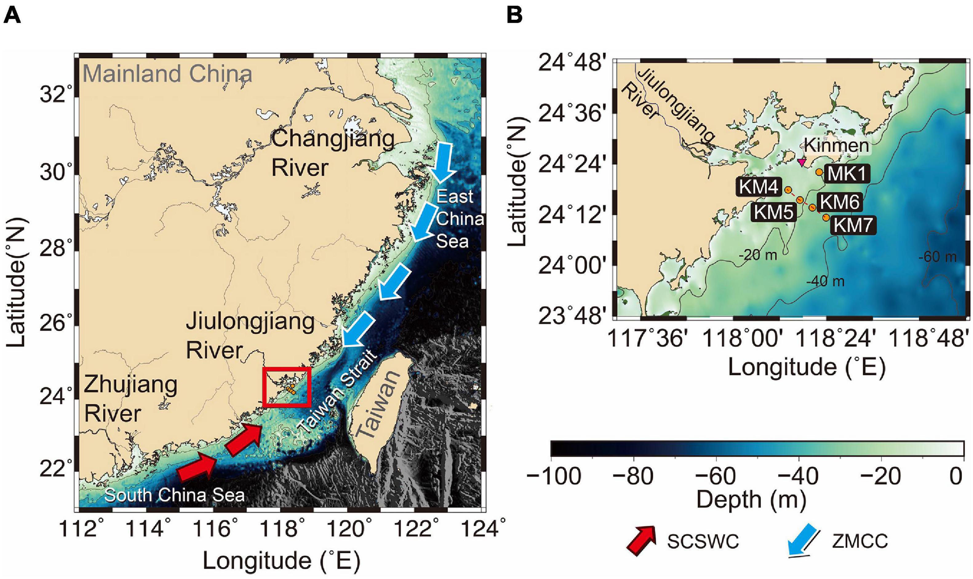
Figure 1. (A) The map showing the Taiwan Strait that links the South China Sea and East China Sea. The red box indicates the location of the study area (Xiamen Bay). Red arrows represent the direction of SCSWC, blue arrows roughly represent the direction of the ZMCC. (B) Enlarged map of the red box showing the fixed sampling station at MK1 and transect stations KM4∼KM7 by orange circles. The bright purple triangle showing the Kinmen Weather Station.

Studies show that the coast-hugging China Coastal Current or Zhejiang (Zhe)-Fujian (Min) Coastal Current (ZMCC) flows southwestward in the western part of the TS in winter, and the northern SCS Warm Current (SCSWC) and Kuroshio Branch Current flow northward to the western and eastern parts of the TS, respectively, in summer (Jan et al., 2002, 2010; Chen, 2003; Hu et al., 2010; Hong et al., 2011b). These surface currents are controlled by seasonal monsoons, which strengthen the northward flow in summer and the southward flow in other seasons (Jan et al., 2002; Zhu et al., 2013). When two water masses of different origins meet, a front is formed due to the contrast in water properties across the boundary (Chen, 2009). Mapped fronts in satellite images of sea surface temperature (SST) and chlorophyll-a have been used to show boundaries of different water masses in the region (Chang et al., 2006; Chen and Wang, 2006; Liu et al., 2019). These fronts also indicate coupling between physics and waterborne properties such as fluorescence and turbidity (Chen, 2009; Liu et al., 2019).

Many shipboard observations of hydrographic surveys, surface drifters for spatial variability, and fixed-point time-series records from moorings, and high-frequency ground wave radar scanning exist (Qiu et al., 2011; Zhu et al., 2013; Du and Liu, 2017; Liu et al., 2019). They reveal that the monsoon or the wind field condition plays an important role in the changes of the currents in the TS. In the nearshore area, apart from different sources of water mass, the contribution of river plume water is significant (Du and Liu, 2017; Liu et al., 2019). The presence and absence of the river plume determines the coastal water-column density structure, which in turn, affects the nepheloid layers. These layers are major pathway of terrigenous and biogenic particles (Du and Liu, 2017).

In central TS, the effluent of the Jiulongjiang River (JLJR) debouches into the western part of the TS in the form of a hypopycnal plume (Wang et al., 2013; Liu et al., 2019). During the southwesterly monsoon, the JLJR effluent has four spatial expansion modes: flowing northward along the coastline, a bidirectional plume spreading concurrently northeastward and southwestward at the same time, extending just out of the Xiamen Bay, and flowing offshore in the northeastward direction (Wang et al., 2013). It is highly likely that the effluent disperses to the northeast into the interior of the TS. Thus, the effluent of JLJR, the ZMCC water, and the SCSWC water forms the basic constituency of water masses on the west side of the TS.

The encounter of ZMCC water and SCSWC water in the TS also induces the exchanges between the two distal fluvial sources of the CJR and the ZJR. The ZMCC and SCSWC in the TS under different monsoon conditions have been well documented in many studies. However, it is not clear how the regime change of the monsoons affects the interaction of two distal fluvial sources in the TS conduit.

The interactions among the different water masses can be delineated by mapping sea-surface temperature fronts from satellite images (Liu et al., 2019). The near-surface current reversals between different seasons can be monitored by High-Frequency Ground Wave Radar system (Zhu et al., 2008). To resolve the entire water column structures, ship-based observations are essential. However, the short window of the monsoon transition has been rarely captured by ship-based surveys.

The goal of this study was to capture the rare occasion of expected monsoon regime change at the key point offshore of JLJR mouth (Figure 1) between May 7 and 10, 2015. It was fortuitus as the spring-summer monsoon transition occurred in the short window in 2015 was captured in this study. In this paper we present detailed background information of water-mass properties at a critical region in central TS to accentuate our observations from the water column and surface sediment to pinpoint the timing of monsoon regime change.

Materials and Methods

Shipboard Monitoring and Sampling

In the short window of monsoon regime change in 2015, a research cruise was conducted on R/V Ocean Researcher III (OR3)-1850 (04:00 May 7–15:00 May 9) near the mouth of JLJR. The observations consisted of shipboard profiling at hourly intervals (10:00 May 7–10:00 May 9) at MK1 and a transect survey (12:00 May 9–15:00 May 9) from KM4 to KM7 (Figure 1).

A CTD rosette (SBE 911plus) was used in hydrographic profiling (salinity, temperature, fluorescence, and DO) at each station. A LISST-100x (Laser in-situ Scatting and Transmissometer, type C) was added to the rosette to record the volume concentration (VC, in μl/l) of 32 size-classes from 0.25 to 500 μm (on a logarithmic scale) of suspended particles. The rosette was lowered at approximately 1 m/s and the LISST-100x sampled at 1-s intervals (taking an average of 10 measurements), resulting in VC profiles of suspended sediment with 1-m resolution in the vertical. Accordingly, other CTD data were synchronized and averaged into 1-m vertical segments. In addition, water samples were collected at the surface, and near-bottom using 10 l Niskin bottles and seafloor surface sediment samples were taken by a SHIPEK Grab (Wildco 860-A10) at 2-h intervals. To obtain the suspended sediment concentrations (SSC, in mg/l) in different size-classes simultaneously, a nested filtration system Catnet was used to filter water samples onboard, having sieves of three mesh sizes of 153, 63, and 10 μm (Hsu and Liu, 2010; Lee et al., 2016). The Catnet and rosette were directly connected through the water pipe, and 10 l of water sample was introduced into the Catnet for filtration. The suspended particles were collected in a 100 ml bottle at the bottom of the three sieves. Other particles that attached to the sieve were washed into the bottle by hand after the Niskin bottles were drained. At this time, the PC case of the Catnet still contains suspended particles smaller than 10 μm, which were emptied into a jug. Those water in the bottles and the jug were further filtered with a GF filter (0.7 μm). Deionized distilled water (DDW) was used to wash the filter paper to remove salt. During the filtration process, DDW was used to rinse carefully to ensure that no particles remained in each step. Afterward, the filters were freeze-dried and weighed to render the SSC of the following size-classes: >153, 63–153, 10–63, and <10 μm. A portion of each surface water sample (100 ml) was placed in liquid nitrogen for rapid freezing and stored at −4°C for nutrient measurements. Realizing that the radioisotopes in the surface sediments were susceptible to disturbance, the SHIPEK Grab was recovered at a rate of less than 0.5 m/s to avoid disturbance. In addition, the surface sediment in the SHIPEK Grab was confirmed with the naked eye that the uppermost part of the sediments was not disturbed due to overturning, slumping, or serious mixing. After confirmation, the sample was taken within a range of 20^∗20 cm² in the center of bucket of the SHIPEK Grab and freezed for radioisotope analysis. The wind field was measured every minute by shipboard anemometer.

After the fixed-point observations, a hydrographic survey was carried out along a transect from seaward of the river mouth to offshore (Stas. KM 4∼7) during the flood tide. In addition, to verify our observations, other measurements for May from 2000 to the present near our stations were obtained from the World Ocean Database (WOD) for comparison (marked by a to j in Figure 2; Boyer et al., 2018).

FIGURE 2

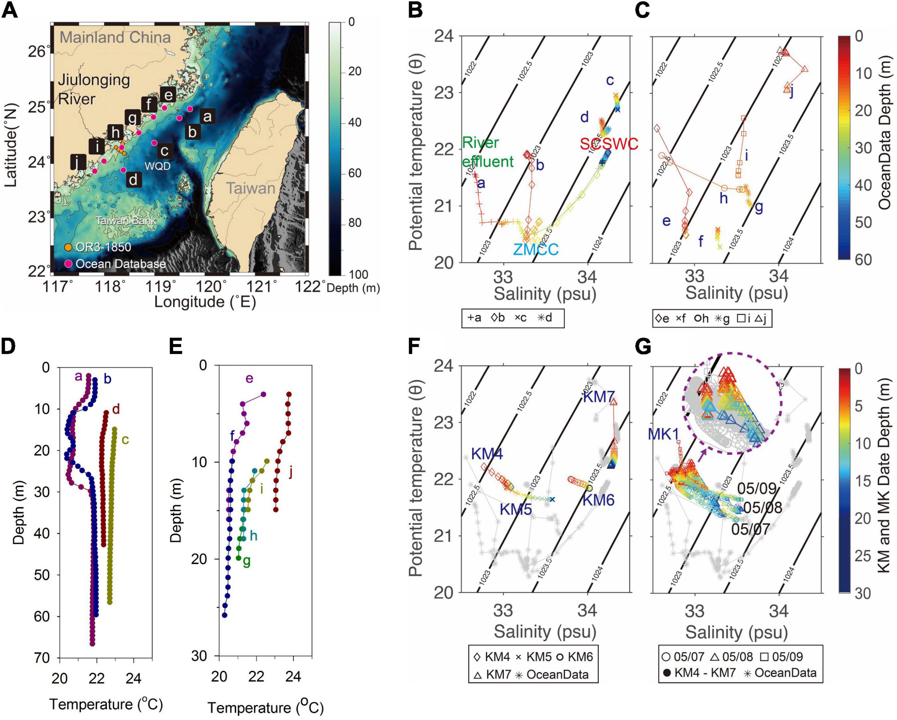
Figure 2. (A) A map showing the WOD data points a∼j. (B) Depth-referenced θ-S diagram at offshore stations a∼d. The surface layer of Sta. a corresponds to coastal water. The middle layer of Sta. a and b corresponds to ZMCC water. Stas. c and d correspond to SCSWC water. (C) Depth-referenced θ-S diagram of near shore stations e∼j. (D) The temperature profiles at a∼d. (E) The temperature profiles at e∼j. (F) Depth-referenced θ-S diagram observed at KM4∼KM7. (G) θ-S diagram observed at KM1 on 5/7∼9 showing circles (5/7), triangles (5/8), and squares (5/9). The temporal changes on 5/8 when the regime change occurred are enlarged in the dashed circle. The θ-S plots in (B,C) are plotted in the background in gray (F,G) to provide perspective to the present data.

The Observations of Suspended Sediments

The volume concentration (VC) of suspended sediments, measured by LISST-100x, were divided into four particle size groups (<10, 10–63, 63–153, >153 ⋅m) corresponding to the partition by the onboard nested filtration system Canet (Lee et al., 2016; Du and Liu, 2017). The SSC obtained by the Catnet was combined with the VC observed by the LISST to calculate the bulk density of suspended sediments follows (Hsu and Liu, 2010). Here ρ_p is the density of primary particles that is assumed 2.65 g/cm³ and ρ_IWis the density of seawater.

$${\mathrm{\rho }}_f={\mathrm{\rho }}_{IW}+\left(1-\frac{{\mathrm{\rho }}_{IW}}{{\mathrm{\rho }}_p}\right)\frac{SSC}{VC}$$

Analyses of Water and Surface Sediment Samples

After the cruise, all samples were analyzed immediately in the laboratory to obtain inorganic nitrogen (NO₃^–, NO₂^–), phosphate (PO₄^3–), and silicate (SiO₂), as well as to measure ²¹⁰Pb_ex and ⁷Be of surface sediments.

The azo dye colorimetric method combining cadmium reduction on flow injection analyzer was used to measure the concentration of nitrate and then calculated nitrate (NO₃^–) by reducing nitrate to nitrite (NO₂^–) (Pai et al., 1990b; Pai and Riley, 1994; Chen et al., 2004). The ascorbic acid/oxalate reduction-colorimetric method on flow injection analyzer was used to measure the concentration of phosphate (PO₄^3–) and silicate (SiO₂) (Pai et al., 1990a; Chen et al., 2004).

After the surface sediment samples were freeze-dried, the water content of the wet sediments was determined. Dried samples were then transferred to plastic jars (inside diameter, 8.5 cm; height, 7.5 cm) for non-destructive gamma-ray spectrometric assay of radionuclides. The data reported in this study were calculated based on salt-free dry weight. Three radionuclides (²¹⁰Pb, ⁷Be, and ²¹⁴Pb) were counted by HPGe detectors connected with the digital gamma-ray spectrometer and analyzed by Gamma Vision 32s software. The detectors can be used to determine ²¹⁰Pb, ²¹⁴Pb and, ⁷Be simultaneously based on photon peaks centered at 46.52, 351.99, and 477.56 keV, respectively (Huh et al., 2009, 2011). The ²¹⁴Pb is the precursor of ²¹⁰Pb and was used as an index of supported ²¹⁰Pb whose activity concentration was subtracted from that of the measured, total ²¹⁰Pb to obtain excess ²¹⁰Pb (²¹⁰Pb_ex) (Su and Huh, 2002; Huh et al., 2009).

The Eigen Function Analysis

A multivariate technique Empirical Orthogonal/Eigen Function (EOF) analysis was used to characterize the correlations (standardized covariability) of variables in the upper water column and near-bottom water column and radioisotopes in seafloor sediment. This technique is based on internal correlations (Resio and Hayden, 1975), which present the statistical characteristics of a group of data through the spatial or temporal correlation of the data (Du and Liu, 2017; Liu et al., 2019; Lee et al., 2021). Each eigenmode in the EOF result was ranked according to the quotient between the eigenvalue of the eigenmode and the sum of all the eigenvalues. The highest mode (mode 1) explains most of the covariability (correlation) in the data set, followed by mode 2, mode 3…etc. In this study, variables in water column at 0∼2 m depth and 0∼2 mab were analyzed separately. Variables from the upper water column included water-mass properties (temperature, salinity, fluorescence, DO, and nutrients), suspended sediment attributes (SSC, VC of four size-groups), tidal height (tidal forcing), and N-S and E-W wind velocity components. In the water-sediment interface, analyzed variables included water-mass properties (temperature, salinity, fluorescence, DO, and nutrients), suspended sediment attributes (SSC, VC of four size-groups), surface sediment proxies (²¹⁰Pb_ex and ⁷Be), tidal height (tidal forcing), and N-S and E-W wind velocity components (Lee et al., 2016, 2021; Liu et al., 2019).

Identifying Fronts in Satellite Sea Surface Temperature Image

Daily images of SST for the TS obtained by NOAA’s AVHRR satellites throughout the year were collected. The entropy-based edge detection method was used to computed front gradient magnitude (GM) using the equation (Chang et al., 2006, 2010): $GM=\sqrt{{(dT/dx)}^2+{(dT/dy)}^2}$ where T is SST, and x and y axes are directed toward east and north, respectively. After computing the GM from all daily image, the monthly mean GM can be obtained. The monthly mean GM map was used to show the frontal patterns and scale the intensity of frontal systems in different month. In this study, to compare the difference of front in each month more clearly, the fronts of different months were digitized and plotted through GMT software.

Results

Time Series Observations

The transition of the seasonal wind field in the TS in 2015 occurred in May as in previous years. At the beginning of April, the wind field was mainly northeast wind, from late April to May were the transition period, and the southwest wind dominated in June (Supplementary Figure 1A). During the transition period, the northeasterly wind alternated with the southwesterly wind. The time series observation was carried out at Sta. MK1 station during this period. One month before the observation period, the wind mainly blew from the northeast between 40 and 70° (Supplementary Figure 1B). One and a half months after the observation period, the wind was mainly from the southwest between 210 and 240° (Supplementary Figure 1C). In this article, the 0° wind direction is defined as the wind blowing from the north, and the wind direction from the east is at 90°. During the time series observation period, the first half was dominated by northeasterly winds and the second half was dominated by southerly winds. The average speed of the northeasterly winds was 4.94 m/s, and the average speed of the southerly wind was 2.69 m/s (Figure 3A). To corroborate with our short shipboard measurement, a longer record (4/9∼6/24) of hourly wind data from the Weather Station on the nearby Kimen Island (Figure 1) and rose diagrams of the wind speed and direction for the NE and SW monsoon periods are shown in Supplementary Figure 1. The data has been averaged for 24-h running mean to reduce the variation due to daily sea and land breezes.

FIGURE 3

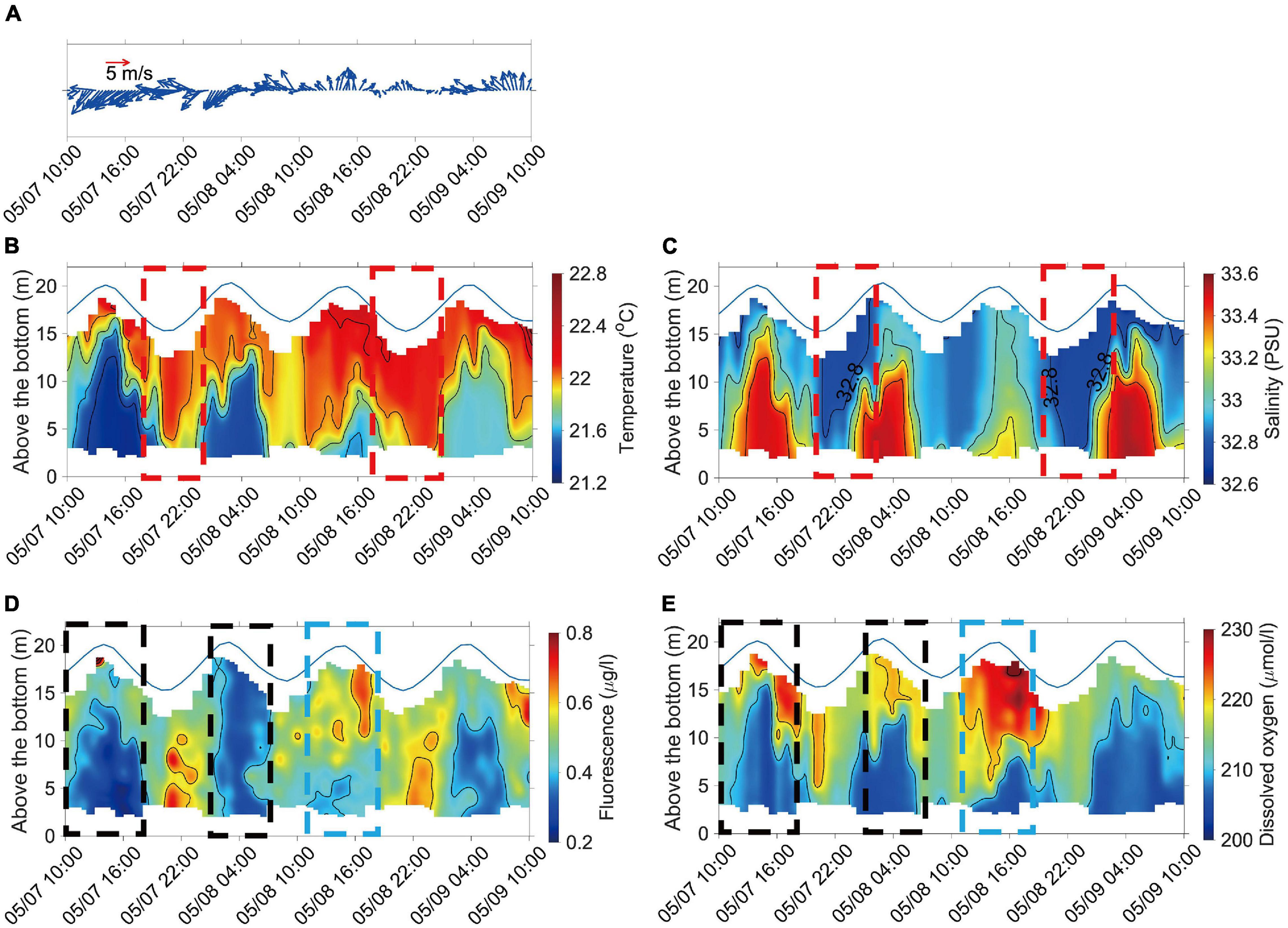
Figure 3. Fixed-point shipboard observations of (A) wind speed and direction (plotted according to the oceanographic convention, north direction is upward, and the scale of the sticks is also shown in the upper left corner; vertical structures of (B) temperature; (C) salinity; (D) fluorescence; (E) dissolved oxygen (DO). The blue curve shows the fluctuations of the water depth. The red dashed rectangles indicate the time of strong river effluent events. The black dashed rectangles indicate vertically well mixed events of fluorescence values. The blue dashed rectangles indicate the corresponding event of fluorescence and DO values.

According to the observed water level, the interval between high tide and low tide was about 12 h, which is a semi-diurnal tidal cycle (two high waters and two low waters each day), and the tidal range was about 5 meters (Figure 3 blue curve). The flood-half tidal cycles referred to the period when the sea level rose from low water to high water, and conversely, the period when sea level dropped from high water to low water level was the ebb-half tidal cycle. A total of 4 full tidal cycles were observed during the time series observation period.

The temperature and salinity structures at Sta. MK1 showed the water column consisted of distinctive surface and bottom layers (Figures 3B,C). Temperature, salinity, fluorescence, and dissolved oxygen (DO) showed strong tidal signals. During flood, the water column was better mixed with warmer, less saline water (Figures 3B,C). During ebb, the water column was stratified due to the presence of colder, more salinity water. However, for two flood-half tidal cycles, the water column was well mixed with high temperature and low salinity water (marked by red dashed boxes in Figures 3B,C), suggesting the influence of river effluent. The fluorescence (Figure 3D) showed different patterns. In general, its values were higher in the surface and lower near the bottom. In one full tidal cycle and one ebb-half tidal cycle (marked by black dashed boxes in Figure 3D), low values existed throughout the water column and remained high in the surface throughout the following tidal cycle. DO values in general were higher in the surface and lower at depth (Figure 3E). There was one episode that high DO coincided with high fluorescence (marked by blue dashed boxes in Figures 3D,E). The temporal changes of the vertical structures of these parameters suggest coupling among physical and biogeochemical processes.

At the surface, the salinity fluctuations were less than 1 PSU (Figure 3C). During the two episodes of river effluent presence (<32.8 PSU, Figure 3C) the nutrient concentrations of NO₃^–, NO₂^–, PO₄^3–, SiO₂, and the volume concentration of suspended sediments increased (Figures 4A,B and Supplementary Figure 2). This indicates JLJR as the source. During flood tide, the effluent was pushed northeastward from the JLJR mouth to reach the MK1 station. The two episodes of river effluent occurred in periods of northeasterly winds and southwesterly winds, respectively. Based on the salinity and the nutrient concentrations, the effluent during the southwesterly winds was stronger than in northeasterly wind period. In addition, the N/P ratio showed gradual decreasing trend during the observation period (Figure 4C).

FIGURE 4

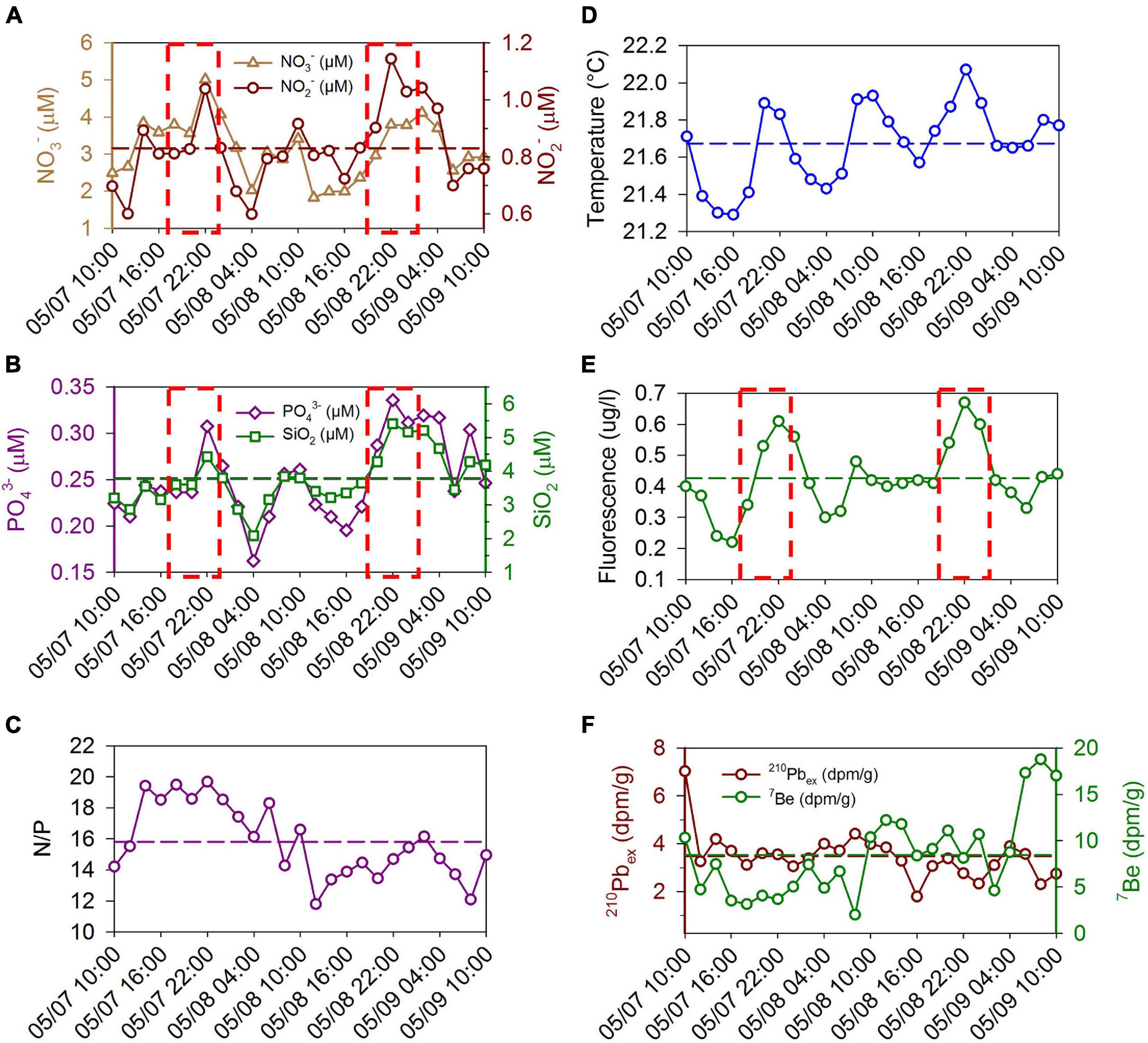
Figure 4. Temporal changes of (A) nitrate and nitrite (NO₃^–, NO₂^–); (B) phosphate (PO₄^3–) and silicate (SiO₂); (C) N/P ratio in the upper water column (dashed line indicates the mean value); and changes of (D) temperature; (E) fluorescence in the lower water column; and (F) ²¹⁰Pb_ex and ⁷Be in the surface sediment. The red rectangles correspond to the dashed red rectangles in Figures 3B,C.

Near the bottom, four tidally modulated intrusion events of low temperature and high salinity water occurred. Each event commenced at the low water through the rising tide, reaching the peak at the high water, and abated during the following falling tide (Figures 3B,C). The intruded water could almost reach the surface, which contained lower fluorescence and lower DO (Figures 3D,E). These associations suggest upwelling (Hu and Wang, 2016). The intrusion of cold and saline water was still present after the wind directions shifted from northeasterly to southerly (Figure 3), suggesting wind was not a major forcing on the local cold-water events. In addition, the temperature, fluorescence of the bottom water and ⁷Be in the surface sediments tended to increase after the wind field change (Figures 4D–F).

Observations of suspended sediment are presented in Supplementary Figures 2, 3. The volume concentration (VC) measurements suggest that the suspended particles larger than 153 μm mainly appeared in the upper water column (Supplementary Figure 2), and the suspended particles smaller than 153 ⋅m appeared near the bottom during river effluent events at Sta. Mk1 (Figure 3C and Supplementary Figure 2). Similarly, river effluent events during the southerly wind have higher SSC than northeasterly wind. SSC of four particle size groups showed that the sediment finer than <10 μm contributed the most to the total SSC both at the surface and near bottom. The peaks in the SSC coincided with the flood tide (Supplementary Figures 3A,B). The bulk density of most suspended particles in the upper water column was higher than that in the lower water column (Supplementary Figures 3C,D and Supplementary Table 1), which may be due to the presence of terrigenous particles delivered by the JLJR effluent. In addition, the bulk density of suspended sediment particle size 63–153 μm in the upper water column increased during the period of cold-water intrusion (Figure 3B and Supplementary Figure 3C). The higher bulk density values suggest that the sediment may be terrigenous material.

Spatial Transect Observations

During the flood tide, a hydrographic transect survey was conducted along Sta. KM4∼KM7 (Figure 1B). In general, the 2-D temperature structure showed relative homogeneous distribution in the vertical at each station. There was a distinct land-to-sea gradient along the transect (Figure 5A). An ascending “cold dome” existed at KM5, indicating the presence of upwelling (Figure 5A). The dominant feature in the salinity structure also showed land-to-sea pattern as the effluent of JLJR encountered the ambient coastal water, forming a frontal zone in the upper water column between KM5 and KM6 where the hypopycnal plume pinched out (Figure 5B). The lower water column was vertically homogeneous between KM4 and KM5 suggesting mixing by currents from below (Liu et al., 2002; Du and Liu, 2017). Coinciding with the “cold dome,” was a “low DO dome” (Figure 5C). Seaward and landward from the low DO dome, high DO areas existed in the surface. High fluorescence layer coexisted with high DO, suggesting the link through primary production (Figures 5C,D). The structural patterns that distinguish salinity from those of temperature and DO indicate different forcing. The salinity pattern was caused by the seaward dispersal of the river effluent as a hypopycnal plume, whereas temperature and DO were mainly affected by the alongshore current transport.

FIGURE 5

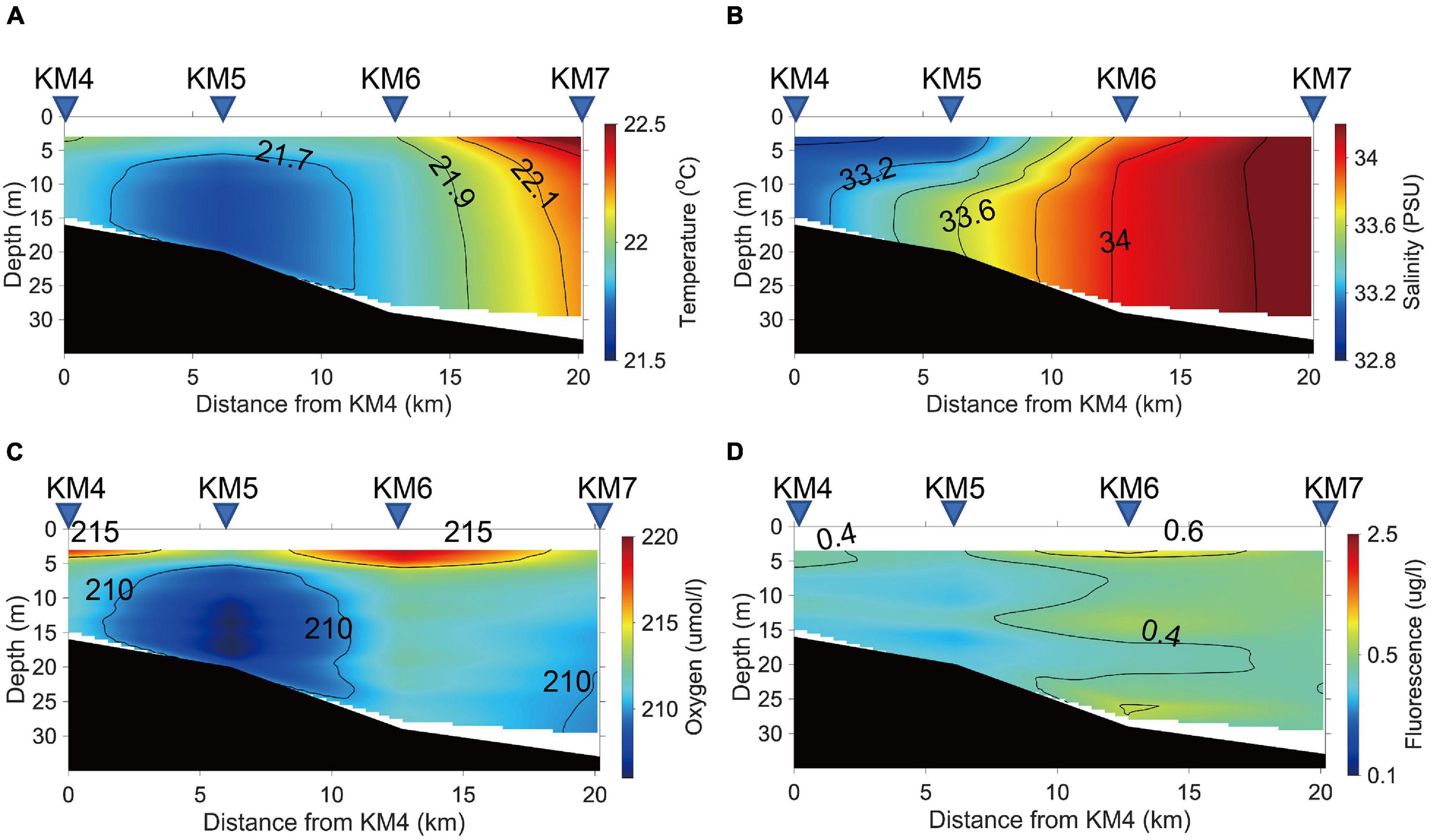
Figure 5. 2-D structures along the transect between KM4 and KM7 of (A) temperature; (B) salinity; (C) DO; (D) fluorescence. The black area represents the sea floor.

According to the characteristics of temperature and salinity along the transect, three different water masses were identified. Firstly, near the river mouth at KM4 was the JLJR plume with the lowest salinity. The second type was the upwelling water with the lowest temperature and DO that occupied the bottom of Sta. KM5. The third type was the ambient water with the highest temperature and salinity in the offshore area at KM7.

Observations of suspended sediments are presented in Supplementary Figure 4. According to the characteristics of VC along the transect (Sta. KM4 to KM7), the 2-D structures of the VC of suspended sediments show size-fractionated spatial patters (Supplementary Figures 4A–D). All four grain sizes show concentrated distributions near the seafloor in the form of a benthic nepheloid layer (BNL). BNLs are a common phenomenon along the coast of Zhejiang and Fujian, mainly formed by the resuspension of seabed sediments (Du and Liu, 2017). The thickness of observed BNL increased with decreasing particle size. The finest size of <10 μm had the thickness of 5∼10 m (Supplementary Figure 4A). Intermediate nepheloid layer (INL) also appeared as extensions of the BNL in deeper depths forming finger-like structures following isopycnals surfaces especially for the two coarser particles (Supplementary Figures 4C,D). All the structures in deeper than 5-m depth seem to display a common land-sea boundary around KM6 that separates the estuarine and coastal influences. However, the finest < 10 and the coarsest > 153 μm sizes also form surface nepheloid layer (SNL) (Supplementary Figures 4A,D). Both SNLs were related to the hypopycnal plume of the JLJR. But the former consisted of fine-grained terrigenous sediment and the latter consisted of biogenic particles (Du and Liu, 2017).

Source of Water Masses

Previous studies show the coastal area near the JLJR mouth is affected by the ZMCC along the coast in winter and the SCSWC in summer (Hu et al., 2010). Different water masses that may be present in the study area were delivered by the effluent of the JLJR, the SCSWC, and the ZMCC. The SCSWC water is warmer and more saline, the ZMCC water is colder and less saline, while the effluent from the JLJR is the least saline (Wang et al., 2013). The latest (2002) May temperature and salinity data from the western part of the TS in the WOD confirm this scenario (Boyer et al., 2018). The temperature is converted to potential temperature (θ) at reference pressure 0 dbar by polynomial fit for adiabatic lapse rate and Runge-Kutta fourth order integration algorithm (Bryden, 1973). The depth-referenced θ-S diagrams of measurements at offshore locations (a, b, c, d) and inshore locations (e, f, g, h, i, j) differentiate the water masses of the two current systems (Figures 2A–C).

Historical data show that along the offshore transect, the surface water is warmer and more saline at stations c and d than that at a and b (Figures 2B,D). Stations c, d are in the shallower part of the TS whereas a, b are in deeper water of the Wuqiu Depression (WQD) (Figure 2A). At c and d, the temperature and salinity are vertically homogenous (Figure 2D). At a and b, the vertical structure shows three segments of mixed layers between surface and 10 m (a and b); 10∼28 m (a), 10∼22 m (b); and 30∼bottom (a), 25∼bottom (b). Thermoclines exist between adjacent segments. On the θ-S diagram the segments are also separated by the salinity. The surface layer is less saline. The middle layer becomes gradually colder and more saline. The bottom layer is the warmest and most saline. The thermohaline coincides with the halocline (Figure 2B).

Along the inshore transect, there is a general southward warming trend from e to j (Figures 2C,E). On the other hand, the water is fresher at e than at j (Figure 2C). In general, at each station, the temperature is more vertically homogeneous. The θ-S characteristics of these selected stations in WOD reveal the signatures and pathways of the water-masses of the warmer and more saline SCSWC and colder, less saline ZMCC.

Boundary of Water Masses

For a broader regional view of the water masse boundary driven by ZMCC and SCSWC, NOAA’s Advanced-Very-High-Resolution-Radiometer (AVHRR) sea-surface temperature (SST) images in the TS were obtained from the regional HRPT Data Library at Tohoku University and National Taiwan Ocean University. Monthly mean values of frontal gradient magnitude were computed (Supplementary Figure 5; Chang et al., 2006). The entropy-based edge detection method was used to describe the SST fronts. Such fronts can represent where different water masses meet. The monthly synthesized fronts were digitized and plotted over the bathymetry to show shifting boundaries between the two systems (Figure 6). From spring to summer, the fronts gradually recede northward in response to the monsoon change. Beginning in winter, the fronts extend southward. The front not only represents the interface of warm and cold-water masses, but also the density gradient between different water masses that prevented the mixing of water and sediment (Qiao et al., 2020). The position of the JLJR mouth seems to be at the southward limit of the retreating front. This phenomenon could be due to the constraint of bathymetry. The WQD accommodated the descending dense warm SCSWC water under the ZMCC water so the front could not progress northward in the surface (Figure 2B).

FIGURE 6

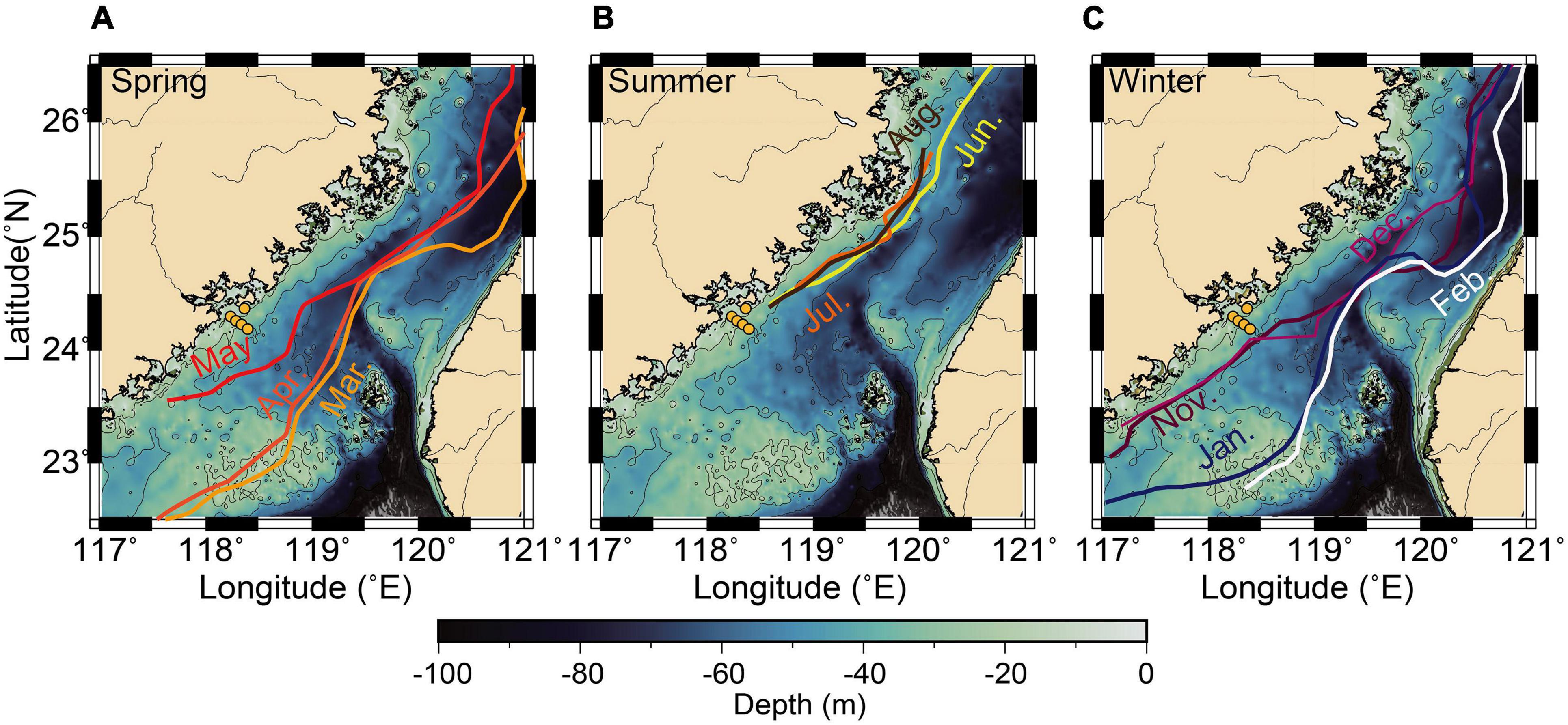
Figure 6. Maps showing the frontal zones digitized from satellite images of monthly SST (Supplementary Figure 4) in (A) spring including March, April, May; (B) summer including Jun, July, Aug.; and (C) winter including Nov., Dec., Jan., Feb. Fronts in September, and October are not clear and thus are not included.

Eigen Function Analysis of Upper Water Column

Finally, EOF analysis was used to examine the covariability among the 19 measured variables at the upper water column (0∼2 m) (Supplementary Figure 6). Results show the first mode explains 37.8% of the standardized covariability (correlation) in the data. The signs of the eigenvectors of this mode show that the tidal height, salinity, temperature and DO are in the negative group whereas the rest of the variables are in the positive group (Figure 7A). The eigenweighting curve of this mode represents the temporal characteristics of this mode showing diurnal inequality in the tidal signals (Figure 7B). This curve mimics the temporal patterns of the variables that have strong tidal signals, including water mass properties, particle attributes, and biogeochemical feedbacks. For illustration, PO₄^3– from the positive group mimics the eigenweighting curve, and salinity from the negative group shows the mirror image of the curve (Figure 7B). Basically, the grouping of this mode indicates that when the values of tidal height and salinity decreased, the values of all other variables (except for the winds) increased. Therefore, this mode is interpreted as the tidally driven coastal water mode, which describes the effluent from the JLJR that transported particles and waterborne substances to the study site during ebb. The mode indicates that tide is the primary physical process to influence the covariability of the measured variables.

FIGURE 7

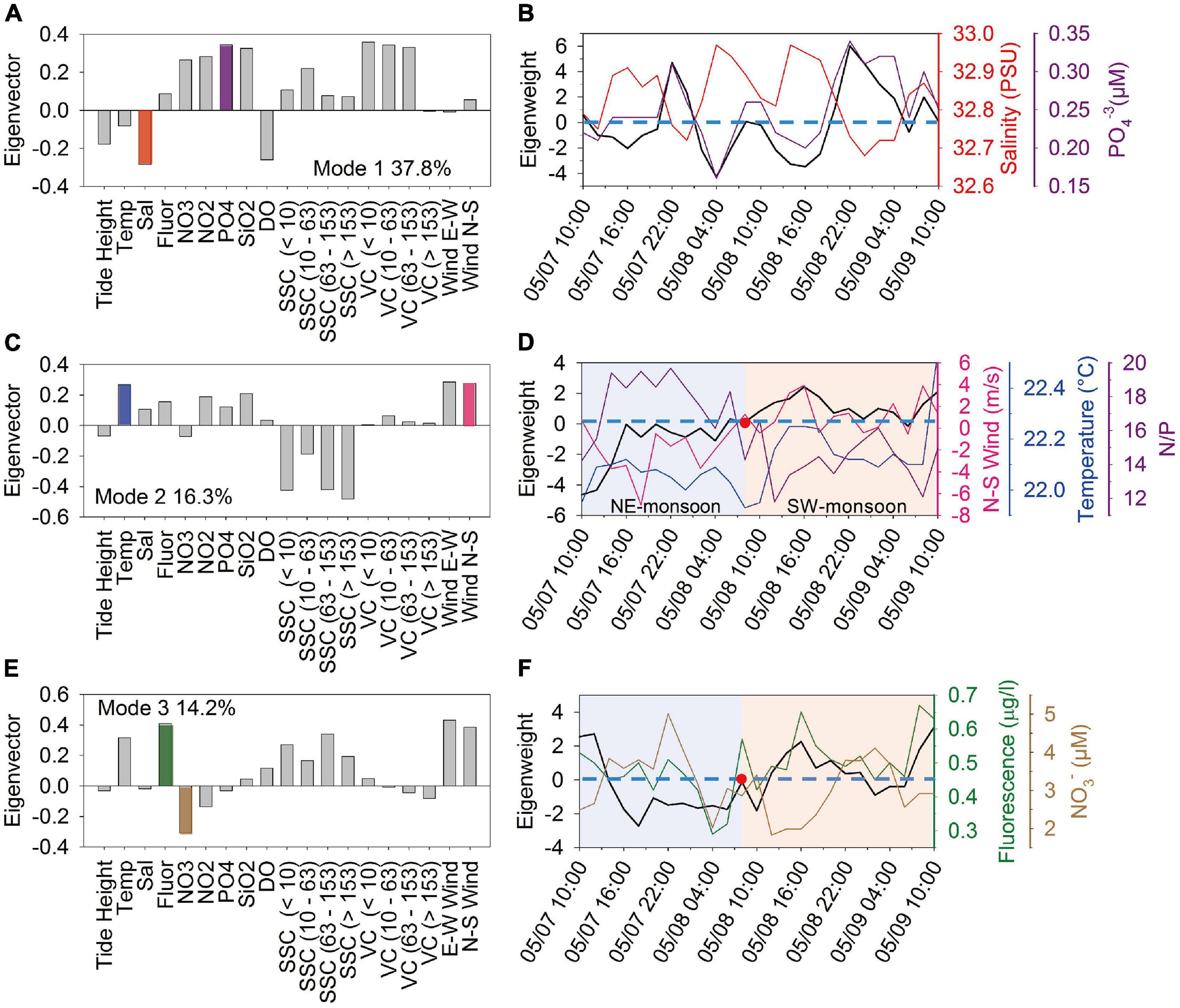
Figure 7. Plots of EOF analysis result on the 19 variables in the upper water column showing (A) Mode 1 eigenvectors; (B) Mode 1 eigenweighting curve with salinity and PO₄^3– as comparison; (C) Mode 2 eigenvectors; (D) Mode 2 eigenweighting curve with N-S wind, temperature, and N/P as comparison; (E) Mode 3 eigenvectors; (F) Mode 3 eigenweighting curve with fluorescence and NO₃^– as comparison (the dotted blue line shows the zero value of the eigenweightings). The red dots show the position of zero-crossing on Mode 2 and 3 eigenweighting curves.

The second mode explains 16.3% covariability in the data. The prominent variables in the positive group are the temperature, salinity, and other variables including all nutrients except for NO₃^–, and the two wind components. The positive grouping indicates that the temperature and salinity increased with the strength of the SW-monsoon (Figure 7C). Comparisons among the eigenweighting curve with the time series of the measured variables show the curve closely mimics the gradually rising temperature (Figure 7D). The zero-crossing time (10:00 on 5/8) of this eigenweighting curve is a demarcation between regimes dominated by the NE-monsoon and SW-monsoon (Figure 7D). Therefore, this mode reflects the monsoon influence. The groupings of this mode indicate that as the surface temperature rose due to the increasing of the SW-monsoon, the SSC and NO₃^– decreased. The SW monsoon drove the SCSWC bringing warmer and low NO₃^– water to the sampling site. When plotting the N/P ratio against the eigenweighting curve of this mode (Figure 7D), one can see the N/P mimics the eigenweighting curve in the NE-monsoon regime but is a mirror image in the SW-monsoon regime. The low N/P values are the characteristics of oligotrophic and nitrogen-limited water from the SCS (Huang et al., 2020). In addition, the upwelling on the southwest side of Taiwan Bank during the SW-monsoon regime also provides some nutrients and are transported northward, especially phosphates, which may also be responsible for the decrease in N/P ratio (Gan et al., 2009; Hong et al., 2011a). Therefore, this mode clearly describes a regime change between the winter and summer monsoons. During this transition, water temperature increased, and N/P and terrestrial SSCs from the ZMCC both decreased.

The third mode explains 14.2% of the covariability. In this mode, the wind components and temperature are the dominant variables in the positive group. Other variables in the possible group include fluorescence and the 4 SSC sizes (Figure 7E). Among variables in the negative group, the two nutrients NO₃^–, NO₂^– are the important ones, of which NO₃^– is the dominant variable. Fluorescence and the two nitrogenous nutrients are in opposite groups indicating the uptake of NO₃^– and NO₂^– by primary producers whose sizes correspond to the 4 SSC sizes. This mode describes the similar scenario as the second mode that the transition in monsoon winds caused the temperature to rise. In this physical setting nitrogenous nutrients were utilized in the production of biogenic particles of the four particle-size classes and increased the fluorescence (Figure 7F). Previous studies show that the uptake of nutrients in phytoplankton production is controlled by the concentration of nitrogen and phosphorus in water masses. The uptake varies depending on the phytoplankton species (Lui and Chen, 2011). Another study also pointed out that low nutrient concentration with high chlorophyll-a concentration is common southwest of Taiwan Bank during summer (Hu et al., 2015). The upwelled water was transported northward. In this water mass, phytoplankton grew rapidly at the favorable temperature, N/P ratio, and sunlight, consuming most of the nutrients (Gan et al., 2009; Hu et al., 2015). Therefore, this model is interpreted as the primary production mode.

Eigen Function Analysis of Bottom Water Column and Surface Sediment

The EOF analysis was also used to examine the covariability among the 17 variables in the bottom water (at 2 m above the bed) and on the seabed (Supplementary Figure 7). Results show the first mode explains 35.2% covariability of the data. The negative group includes salinity, DO, and ²¹⁰Pb_ex. The other variables are all in the positive group including temperature, fluorescence, all particle attributes, ⁷Be, and wind velocities (Figure 8A). Since temperature and salinity are in opposite groups, this mode describes the influence of JLJR effluent driven by the NE-directed monsoon winds. Also, fluorescence and all particle attributes are opposite to salinity, implying primary producers of all sizes are associated with the effluent. The eigenweighting curve of this mode shows an increasing secular trend along tidal oscillations (Figure 8B), indicating increases in value of variables in the positive group (illustrated by temperature and fluorescence plotted in Figures 4D,E).

FIGURE 8

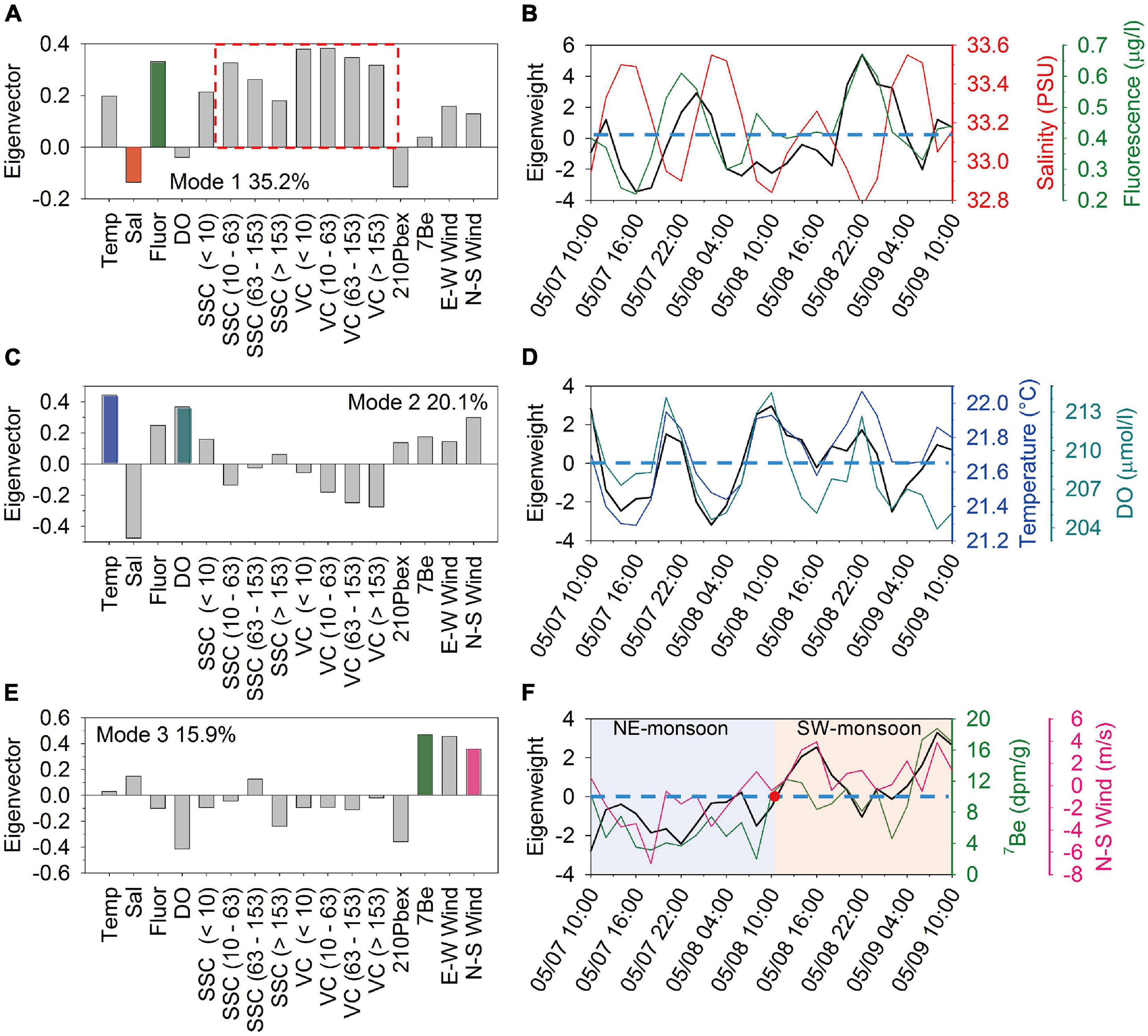
Figure 8. Plots of EOF analysis result on the 16 variables in the lower water column and in the surface sediment showing (A) Mode 1 eigenvectors (the red dashed box show the suspended sediment attributes); (B) Mode 1 eigenweighting curve with salinity and fluorescence as comparison; (C) Mode 2 eigenvectors; (D) Mode 2 eigenweighting curve with temperature and DO as comparison; (E) Mode 3 eigenvectors; (F) Mode 3 eigenweighting curve with ⁷Be and N-S wind as comparison (the dotted blue line shows the zero value of the eigenweightings). The red dot shows the position of zero-crossing on Mode 3 eigenweighting curve.

The second model explains 20.1% covariability. The temperature and salinity are also in opposite groups. This mode describes the effect of cold-water intrusion (Figure 8C). The negative portions of the eigenweighting curve of this mode (Figure 8D) correspond to episodes of low temperature, high salinity, and low DO near the seabed (Figures 3B,C,E). As a result, the eigenweighting curve of this mode mimics the temporal changes of temperature and DO very well (Figure 8D). However, fluorescence and surface sediment proxies of ²¹⁰Pb_ex, ⁷Be co-varied inversely with the salinity, suggesting their riverine association.

The third model explains 15.9% of the covariability which is dominated by ⁷Be and the two wind-velocity components in the positive group (Figure 8E). DO and ²¹⁰Pb_ex covaried inversely in the negative group. The eigenweighting curve of this mode shows a pronounced increasing secular trend that mimics the temporal changes of ⁷Be and the N-S wind velocity well (Figure 8F). The grouping of this mode points out when the southwesterly monsoon wind strengthened, in the surface sediment the ⁷Be concentration increased and ²¹⁰Pb_ex activities decreased, and the DO in the bottom water decreased (Figures 8E,F).

Discussion

Based on previous studies and the θ-S characteristics of water masses from WOD in this study (Hu et al., 2010; Zhu et al., 2013), the ZMCC is coastal hugging, flowing southward along the inshore area near the coastline. The SCSWC, flows over the Taiwan Bank and follows along the WQD (Figure 2A). At Station a and b, the two current systems encounter each other. At the surface the upper 10 m is occupied by the coastal water. Since the ZMCC water mass is the coldest, it formed the colder and less saline middle mixed layer between 10 and 30 m. The warmer SCSWC water mass occupied the lower part of the water column below 30 m. Similar water mass structures have been described in previous studies in the northern TS and the ECS (Du and Liu, 2017; Wu et al., 2021). Within this overall setting, along the transport route of the ZMCC, the colder and more saline water at f and g than at e and h (Figures 2C,E) might be caused by coastal upwelling as described by Liu et al. (2019). Additionally, the fresher and warmer water in the upper water column creating stratification might be caused by the river effluent from the JLJR (at h) and Mulanxi River (at e) (Figure 2C).

Having established the spatial patterns of properties of the coastal water masses and current systems on the western side of the TS, we now put our observations in perspective. The surface layer at KM4 and KM5 closer to the mouth of the JLJR was the river effluent water, and the values of salinity and temperature in the bottom layers were in between those of SCSWC and ZMCC following isopycnals (Figure 2F), indicating the mixing of the SCSWC and ZMCC. At KM6, the θ-S signals of surface water were between the SCSWC water and the ZMCC water, while the bottom layer were almost the values of the SCSWC water (Figure 2F). At KM7, the θ-S signals of the surface and bottom layers were identical to those of the SCSWC water, indicating that the influence of the SCSWC became stronger farther away from the river/land.

The observed shipboard time series are also plotted on the θ-S diagram to show the same perspective (Figure 2G). The θ-S signal characteristics at the MK1 station are like those at the KM4 and KM5 stations, showing influence of the JLJR effluent in the upper water column and the mixed water of the SCSWC and the ZMCC in the lower water column. Comparing with KM4 and KM5, the bottom water at MK1 was closer to that of the ZMCC, due to the stronger influence of ZMCC. The fixed-point θ-S profile observations at MK1 are marked according to the date. The data show that the bottom θ-S signals gradually deviated from that of ZMCC as the wind field changed to southerly on May 8. Specifically, from 10:00 to 18:00 on May 8, with the strengthening of the southwesterly wind, the θ-S signals of the entire water column turned closer to that of the SCSWC (Figure 2G).

Through EOF results, the measured variables near the JLJR mouth were mainly controlled by the tidally driven river effluent. Secondly, EOF results reflects the duel between the ZMCC and SCSWC under the dominance of monsoon. Previous studies have classified the diffusion patterns of JLJR plume water within two meters of the surface (Wang et al., 2013). High-frequency ground wave radar scanning results also explain the reversal of the flow field dominated by the monsoon (Zhu et al., 2008). However, the influencing factors such as tides and monsoon winds on the variations of water properties is still unclear.

In fact, from the percentage of explained eigenmodes, the tide played an important role in the variability of water properties. During a tidal cycle, the effluent of JLJR spreads northeastward in the flood tide. During ebb, the southwestward flow caused the mixed water of the ZMCC and the SCSWC to intrude into the lower water column at MK1 station. However, in the offshore area (beyond 25 m isobath), the influence of tides and river effluent was weakened, the θ-S signature was determined by the duel between the ZMCC and SCSWC. Due to the offshore topography, the ZMC and the SCSWC water masses did not fully mix, and the dense SCSWC water sank under the ZMCC water. If the transect of KM4-KM7 was used as the boundary, south of this boundary the SCSWC dominated the θ-S characteristics. North of this boundary a three-layered structure existed. The lower part (deeper than 25 m) of the water column was mainly affected by the SCSWC. The middle part (10–25 m) was affected by the ZMCC and the upper part by the river effluent. River effluent is also affected by rainfall and other factors, so it does not necessarily continue to exist on the surface. Therefore, the monthly average temperature front is a result of the duel between ZMCC and SCSWC.

The changes of monsoons determined the outcome of the duel between ZMCC and SCSWC, and affected the changes of the water properties offshore JLJR mouth on a longer time scale. The zero-crossing of the eigenweighting curves in the EOF analysis results can clearly illustrate such a change. The zero-crossing of the second mode in the surface water data set occurred on 10:00 May 8, which was the same time as that of that of the third mode in the bottom water data set. This coincidence points out a significant phenomenon and yet has not been discovered before.

In the surface water, the southwesterly monsoon winds enhanced the strength of the SCSWC, which had lower N/P ratio, causing a secular decreasing trend in the surface water (Figure 4C). On the other hand, the weakening of the northeasterly monsoon winds weakened the ZMCC, which carried colder water having higher N/P ratio (Chen, 2003). The covarying changes in the temporal waterborne properties caused by the monsoon regime change were captured by the second eigenmode and the exact timing of the regime change occurred on 10:00 May 8 (Figures 7C,D). At the MK1 station, although the tide was the dominant forcing affecting the water column stratification and waterborne properties, there was a warming trend by the SCSWC water in the upper water column (dashed circle in Figure 2G) toward the end of the shipboard monitoring.

On the sediment-water interface, the effect of the regime change was described by the third eigenmode (Figures 8E,F). This mode is dominated by two fine-grained sediment tracers of ²¹⁰Pb_ex and ⁷Be in opposite groups. ²¹⁰Pb_ex in coastal waters is supplied by ocean water, riverine export, in situ decay of ²²⁶Ra, and atmospheric fallout (Dukat and Kuehl, 1995; Sommerfield et al., 2007). ²¹⁰Pb_ex is due to the scavenging effect of fine-grained particles to remove ²¹⁰Pb in the water column (Huh and Su, 1999; Baskaran and Santschi, 2002). The values of ²¹⁰Pb_ex are largely determined by the supply and duration of the scavenging process (Huh and Su, 1999; Su and Huh, 2002). ⁷Be on the other hand, often indicates fresh terrestrial sediment related to storm rainfall and river flood events (Allison et al., 2005; Sommerfield et al., 2007; Liu et al., 2013). Because of its short half-life (53 days), in marine environments, ⁷Be can be detected only in freshly deposited terrestrial sediment less than about 200 days old (Huh et al., 2011; Du et al., 2012). Spatially, the longer the fluvial sediment gets transported away from the riverine source, the weaker the ⁷Be signals become (Liu et al., 2018).

In this study, the two distal fluvial sources, the ZJR and the CJR, are 600 and 900 km away from the JLJR, respectively, and the effluent of JLJR was weak during the observation period. Therefore, the change of ⁷Be concentration in surface sediment can exclude the effect of proximal terrestrial source, mainly due to the sorption of ⁷Be by the particles in surface water. With the monsoon regime change, the fluorescence and the VC of large particle increased simultaneously, indicating that these large particles may belong to biological particles (Supplementary Figure 6). Compared with ²¹⁰Pb, which can always be removed from seawater by particles, ⁷Be scavenging in surface seawater requires more particles (²¹⁰Pb has a higher sorption distribution coefficient than that of ⁷Be for suspended matter) (Allison and Allison, 2005). Previous studies have also shown that the sorption of all radionuclides was significantly enhanced in the presence of organic particles, and the sorption of ⁷Be by organic particles is the most significant (Chuang et al., 2014).

The demarcation between monsoon regimes illustrated by the zero-crossing eigenweighting curves (Figure 8F) is further illustrated by the plot of the temporal changes in ⁷Be/²¹⁰Pb_ex (Supplementary Figure 8). The time-averaged value is indicated by the dashed line which intercepts with the ⁷Be/²¹⁰Pb_ex curve at the same demarcation time of 10:00 on May 8. Before and after this time point, the ⁷Be/²¹⁰Pb_ex values are below and above the average, respectively. This transition indicates the switch of water masses increases the biological particles (fluorescence increased in the upper water, Supplementary Figure 9). These particles adsorbed more ⁷Be to the bottom, which in turn led to a transition in the bottom sediments (Supplementary Figure 9). The monsoon regime change not only directly affects the properties of the water masses, but also indirectly affects the properties of the surface sediments.

The effects of river effluent, tides and monsoon winds on water borne properties on the diurnal to 3-day time scales have been quantified by the EOF analysis. Findings of this study are further illustrated in three schematic diagrams (Figure 9). Monsoon winds were the primary drivers of all the changes described in this study. The Southbound ZMCC was enhanced by northwesterly monsoon winds to have stronger magnitude and wider spread into the TS, forming a strong vertical front at the seaward boundary (Figure 9A). Cold and less saline water masses were driven southward carrying terrestrial sourced and suspended biogenic and clastic particles. In the upper water column, the water masses carried terrestrial sourced nutrients with higher N/P ratio from ECS and higher DO (Figure 4C and Supplementary Figure 6). Cold and saline water was also transported landward in the lower water column modulated by the tide.

FIGURE 9

Figure 9. Schematic presentations of how the monsoon regime change affected land-ocean interactions in the western side of the TS. Bold blue and red arrows represent the NE and SW monsoon winds. Flow symbols on the side of each block facing the page show ZMCC coming out of the page (southbound) and SCSWC going into the page (northbound). Translucent red and blue color blocks represent SCSWC and ZMCC water masses and the solid light blue represents JLJR water, respectively. The inverse triangle shows the location of MK1 station. The black dotted line marks the approximate location of the SST front between ZMCC and SCSWC. (A) Under NE monsoon dominance in winter, ZMCC water occupies the upper water column, the SCSWC water is in deeper layer and is seaward of the ZMCC water. (B) In the transitional period of the regime change in spring, the ZMCC water recedes northward and shoreward and begin to mix with the encroaching SCSWC water from the south and from below. The dispersal of the effluent of JLJR parallels the front between the ZMCC and SCSWC. (C) Under SW monsoon dominance in summer, SCSWC water almost occupies the entire nearshore water column. River plume water replaces the ZMCC water at the surface near the coast. Traces of ZMCC water can still be seen.

During the short window of 3 days, the monsoon regimes changed from NE dominance to SW dominance on May 8 at 10:00. The wind field changed abruptly. Temperature in the lower water column quickly warmed up (Figures 3B, 9B). As the SW-monsoon assumed dominance, the frontal zone between the water masses of ZMCC and SCSWC began to retreat northward and landward (Figures 6A,B). A front was also formed between the ZMCC and the encroaching SCSWC at the location of Sta. MK6. In addition, the JLJR effluent became weakened as it was dispersed farther seaward (Figures 5B, 9B). Near the mouth of JLJR, water masses of the river effluent, ZMCC, and SCSWC occupied different depths in the water column and interacted with one another in a complex manner. In the on-offshore direction, the brackish effluent pinched out on the saline SCSWC water at the surface. However, the brackish effluent and the less saline ZMCC were indistinguishable. They could be distinguished from the warmer SCSWC water only by temperature (Figure 5).

During the SW-monsoon regime, warm water masses occupied the entire water column except for the narrow nearshore zone (Figure 9C). Nutrients in upper water column had lower N/P ratio but higher primary production (Figures 4C, 7E). The frontal zone between the water masses of ZMCC and SCSWC retreated farther northward (Figure 9C).

Conclusion

In conclusion, water masses off the mouth of JLJR can be roughly distinguished into coastal water containing river effluent, the ZMCC water, and the SCSWC water during the study period. In the nearshore area, coastal water dominated the surface, and the bottom is dominated by the mixture of ZMCC and SCSWC water masses. The influence of coastal water is weakened in the offshore (beyond 25-m isobath) where the ZMCC and SCSWC meet. The seaward extension from the JLJR mouth to offshore is roughly a physical boundary during the period of monsoon regime change. South of the boundary the SCSWC water dominates the water column, and north of this boundary ZMCC water dominates. When the two water masses meet, the denser SCSWC flows northward, sinks under the ZMCC. Spatially, the frontal boundary of the two water masses changes with the seasons. Overall, physical processes that affect the area in the western part of the TS near the JLJR mouth are the river effluent dispersal and tidal motions on smaller spatial scales. On larger spatial scales the monsoon winds dominate the ZMCC and SCSWC and the water masses they carry. In this setting, our study reveals the critical period when the regime change occurred, which not only affected land-sea interaction in the physics and biology coupling in the proximal area of the site, but also the alternating dominance of terrestrial signals of the two major distal fluvial sources.

Data Availability Statement

The raw data supporting the conclusions of this article will be made available by the authors, without undue reservation.

Author Contributions

JL conceived and designed the study, supervised the work, and co-wrote the manuscript. RY participated in the cruise design, onboard sampling, and sample analyses, plotted and interpreted the data, and co-wrote the manuscript. C-CS contributed to the analysis of the radio isotopes and data interpretation. YC did temperature gradient magnitude computation and plotting from composite satellite sea-surface data and interpretation. JX digitized front from gradient magnitude plots and frontal interpretation. H-KL contributed to the nutrient data interpretation. All authors contributed to the article and approved the submitted version.

Funding

This study was funded by the ROC Ministry of Science and Technology (MOST) under grant nos. MOST 104–2611-M-110–011, MOST 108-2611-M-110-011–, and MOST 109-2611-M-110-014- to JL.

Conflict of Interest

The authors declare that the research was conducted in the absence of any commercial or financial relationships that could be construed as a potential conflict of interest.

Publisher’s Note

All claims expressed in this article are solely those of the authors and do not necessarily represent those of their affiliated organizations, or those of the publisher, the editors and the reviewers. Any product that may be evaluated in this article, or claim that may be made by its manufacturer, is not guaranteed or endorsed by the publisher.

Acknowledgments

We appreciate the help of Chen-Tung Arthur Chen’s Laboratory in the Department of Oceanography for nutrient analysis, National Sun Yat-sen University. We thank the two reviewers for their helpful comments and suggestions to improve the manuscript.

Supplementary Material

The Supplementary Material for this article can be found online at: https://www.frontiersin.org/articles/10.3389/fmars.2021.735242/full#supplementary-material

References

Allison, J. D., and Allison, T. L. (2005). Partition Coefficients for Metals in Surface Water, Soil, and Waste. Washington, DC: U.S. Environmental Protection Agency, 74.

Google Scholar

Allison, M. A., Sheremet, A., Goni, M. A., and Stone, G. W. (2005). Storm layer deposition on the Mississippi-Atchafalaya subaqueous delta generated by Hurricane Lili in 2002. Cont. Shelf Res. 25, 2213–2232. doi: 10.1016/j.csr.2005.08.023

CrossRef Full Text | Google Scholar

Bai, Y., He, X. Q., Pan, D. L., Chen, C. T. A., Kang, Y., Chen, X. Y., et al. (2014). Summertime Changjiang River plume variation during 1998-2010. J. Geophys. Res. Oceans 119, 6238–6257. doi: 10.1002/2014jc009866

CrossRef Full Text | Google Scholar

Bai, Y., Huang, T. H., He, X. Q., Wang, S. L., Hsin, Y. C., Wu, C. R., et al. (2015). Intrusion of the Pearl River plume into the main channel of the Taiwan Strait in summer. J. Sea Res. 95, 1–15. doi: 10.1016/j.seares.2014.10.003

CrossRef Full Text | Google Scholar

Baskaran, M., and Santschi, P. H. (2002). Particulate and dissolved Pb-210 activities in the shelf and slope regions of the Gulf of Mexico waters. Cont. Shelf Res. 22, 1493–1510. doi: 10.1016/s0278-4343(02)00017-1

CrossRef Full Text | Google Scholar

Berdeal, I. G., Hickey, B. M., and Kawase, M. (2002). Influence of wind stress and ambient flow on a high discharge river plume. J. Geophys. Res. Oceans 107:24. doi: 10.1029/2001jc000932

CrossRef Full Text | Google Scholar

Boyer, T. P., Baranova, O. K., Coleman, C., Garcia, H. E., Grodsky, A., Locarnini, R. A., et al. (2018). “World Ocean Database 2018”. A.V. Mishonov, Technical Ed. Silver Spring, MD: NOAA.

Google Scholar

Bryden, H. L. (1973). New polynomials for thermal expansion, adiabatic temperature gradient and potential temperature of sea water. Deep Sea Res. Oceanogr. Abstr. 20, 401–408. doi: 10.1016/0011-7471(73)90063-6

CrossRef Full Text | Google Scholar

Chang, Y., Shieh, W. J., Lee, M. A., Chan, J. W., Lan, K. W., and Weng, J. S. (2010). Fine-scale sea surface temperature fronts in wintertime in the northern South China Sea. Int. J. Remote Sens. 31, 4807–4818. doi: 10.1080/01431161.2010.485146

CrossRef Full Text | Google Scholar

Chang, Y., Shimada, T., Lee, M. A., Lu, H. J., Sakaida, F., and Kawamura, H. (2006). Wintertime sea surface temperature fronts in the Taiwan Strait. Geophys. Res. Lett. 33:4. doi: 10.1029/2006gl027415

CrossRef Full Text | Google Scholar

Chen, C. T. A. (2003). Rare northward flow in the Taiwan Strait in winter: a note. Cont. Shelf Res. 23, 387–391. doi: 10.1016/s0278-4343(02)00209-1

CrossRef Full Text | Google Scholar

Chen, C. T. A. (2009). Chemical and physical fronts in the Bohai, Yellow and East China Seas. J. Mar. Syst. 78, 394–410. doi: 10.1016/j.jmarsys.2008.11.016

CrossRef Full Text | Google Scholar

Chen, C. T. A., Hsing, L. Y., Liu, C. L., and Wang, S. L. (2004). Degree of nutrient consumption of upwelled water in the Taiwan Strait based on dissolved organic phosphorus or nitrogen. Mar. Chem. 87, 73–86. doi: 10.1016/j.marchem.2004.01.006

CrossRef Full Text | Google Scholar

Chen, M. J., Pattiaratchi, C. B., Ghadouani, A., and Hanson, C. (2019). Seasonal and inter-annual variability of water column properties along the Rottnest continental shelf, south-west Australia. Ocean Sci. 15, 333–348. doi: 10.5194/os-15-333-2019

CrossRef Full Text | Google Scholar

Chen, T. A., and Wang, S. L. (2006). A salinity front in the southern East China Sea separating the Chinese coastal and Taiwan Strait waters from Kuroshio waters. Cont. Shelf Res. 26, 1636–1653. doi: 10.1016/j.csr.2006.05.003

CrossRef Full Text | Google Scholar

Chuang, C. Y., Santschi, P. H., Jiang, Y. L., Ho, Y. F., Quigg, A., Guo, L. D., et al. (2014). Important role of biomolecules from diatoms in the scavenging of particle-reactive radionuclides of thorium, protactinium, lead, polonium, and beryllium in the ocean: a case study with Phaeodactylum tricornutum. Limnol. Oceanogr. 59, 1256–1266. doi: 10.4319/lo.2014.59.4.1256

CrossRef Full Text | Google Scholar

Corbett, D. R., Mckee, B., and Duncan, D. (2004). An evaluation of mobile mud dynamics in the Mississippi River deltaic region. Mar. Geol. 209, 91–112. doi: 10.1016/j.margeo.2004.05.028

CrossRef Full Text | Google Scholar

Dagg, M., Benner, R., Lohrenz, S., and Lawrence, D. (2004). Transformation of dissolved and particulate materials on continental shelves influenced by large rivers: plume processes. Cont. Shelf Res. 24, 833–858. doi: 10.1016/j.csr.2004.02.003

CrossRef Full Text | Google Scholar

Du, J. Z., Zhang, J., and Baskaran, M. (2012). “Applications of short-lived radionuclides (7Be, 210Pb, 210Po, 137Cs and 234Th) to trace the sources, transport pathways and deposition of particles/sediments in rivers, estuaries and coasts,” in Handbook of Environmental Isotope Geochemistry, Vol.I, ed. M. Baskaran (Berlin: Springer Berlin Heidelberg), 305–329.

Google Scholar

Du, X. Q., and Liu, J. T. (2017). Particle dynamics of the surface, intermediate, and benthic nepheloid layers under contrasting conditions of summer monsoon and typhoon winds on the boundary between the Taiwan Strait and East China Sea. Prog. Oceanogr. 156, 130–144. doi: 10.1016/j.pocean.2017.06.009

CrossRef Full Text | Google Scholar

Dukat, D. A., and Kuehl, S. A. (1995). Non-steady-state 210Pb flux and the use of 228Ra/226Ra as a geochronometer on the Amazon continental shelf. Mar. Geol. 125, 329–350. doi: 10.1016/0025-3227(95)00018-t

CrossRef Full Text | Google Scholar

Gan, J. P., Cheung, A., Guo, X. G., and Li, L. (2009). Intensified upwelling over a widened shelf in the northeastern South China Sea. J. Geophys. Res. Oceans 114:15. doi: 10.1029/2007jc004660

CrossRef Full Text | Google Scholar

Hong, H. S., Chai, F., Zhang, C. Y., Huang, B. Q., Jiang, Y. W., and Hu, J. Y. (2011a). An overview of physical and biogeochemical processes and ecosystem dynamics in the Taiwan Strait. Cont. Shelf Res. 31, S3–S12. doi: 10.1016/j.csr.2011.02.002

CrossRef Full Text | Google Scholar

Hong, H. S., Liu, X., Chiang, K. P., Huang, B. Q., Zhang, C. Y., Hu, J., et al. (2011b). The coupling of temporal and spatial variations of chlorophyll a concentration and the East Asian monsoons in the southern Taiwan Strait. Cont. Shelf Res. 31, S37–S47. doi: 10.1016/j.csr.2011.02.004

CrossRef Full Text | Google Scholar

Hopkins, J., Lucas, M., Dufau, C., Sutton, M., Stum, J., Lauret, O., et al. (2013). Detection and variability of the Congo River plume from satellite derived sea surface temperature, salinity, ocean colour and sea level. Remote Sens. Environ. 139, 365–385. doi: 10.1016/j.rse.2013.08.015

CrossRef Full Text | Google Scholar

Hsieh, H. Y., Yu, S. F., and Lo, W. T. (2013). Influence of monsoon-driven hydrographic features on siphonophore assemblages in the Taiwan Strait, western North Pacific Ocean. Mar. Freshw. Res. 64, 348–358. doi: 10.1071/mf12151

CrossRef Full Text | Google Scholar

Hsu, R. T., and Liu, J. T. (2010). In-situ estimations of the density and porosity of flocs of varying sizes in a submarine canyon. Mar. Geol. 276, 105–109. doi: 10.1016/j.margeo.2010.07.003

CrossRef Full Text | Google Scholar

Hu, J., Lan, W. L., Huang, B. Q., Chiang, K. P., and Hong, H. S. (2015). Low nutrient and high chlorophyll a coastal upwelling system–a case study in the southern Taiwan Strait. Estuar. Coast. Shelf Sci. 166, 170–177. doi: 10.1016/j.ecss.2015.05.020

CrossRef Full Text | Google Scholar

Hu, J. Y., Kawamura, H., Li, C. Y., Hong, H. S., and Jiang, Y. W. (2010). Review on current and seawater volume transport through the Taiwan Strait. J. Oceanogr. 66, 591–610. doi: 10.1007/s10872-010-0049-1

CrossRef Full Text | Google Scholar

Hu, J. Y., and Wang, X. H. (2016). Progress on upwelling studies in the China seas. Rev. Geophys. 54, 653–673. doi: 10.1002/2015rg000505

CrossRef Full Text | Google Scholar

Hu, L. M., Shi, X. F., Yu, Z. G., Lin, T., Wang, H. J., Ma, D. Y., et al. (2012). Distribution of sedimentary organic matter in estuarine-inner shelf regions of the East China Sea: implications for hydrodynamic forces and anthropogenic impact. Mar. Chem. 142, 29–40. doi: 10.1016/j.marchem.2012.08.004

CrossRef Full Text | Google Scholar

Hu, Z. F., Qi, Y. Q., He, X. Q., Wang, Y. H., Wang, D. P., Cheng, X. H., et al. (2019). Characterizing surface circulation in the Taiwan Strait during NE monsoon from Geostationary Ocean Color Imager. Remote Sens. Environ. 221, 687–694. doi: 10.1016/j.rse.2018.12.003

CrossRef Full Text | Google Scholar

Huang, T. H., Chen, C. T. A., Bai, Y., and He, X. Q. (2020). Elevated primary productivity triggered by mixing in the quasi-cul-de-sac Taiwan Strait during the NE monsoon. Sci. Rep. 10:9. doi: 10.1038/s41598-020-64580-6

PubMed Abstract | CrossRef Full Text | Google Scholar

Huang, T. H., Chen, C. T. A., Zhang, W. Z., and Zhuang, X. F. (2015). Varying intensity of Kuroshio intrusion into Southeast Taiwan Strait during ENSO events. Cont. Shelf Res. 103, 79–87. doi: 10.1016/j.csr.2015.04.021

CrossRef Full Text | Google Scholar

Huh, C. A., Chen, W. F., Hsu, F. H., Su, C. C., Chiu, J. K., Lin, S., et al. (2011). Modern (<100 years) sedimentation in the Taiwan Strait: rates and source-to-sink pathways elucidated from radionuclides and particle size disttibution. Cont. Shelf Res. 31, 47–63. doi: 10.1016/j.csr.2010.11.002

CrossRef Full Text | Google Scholar

Huh, C. A., Lin, H. L., Lin, S., and Huang, Y. W. (2009). Modern accumulation rates and a budget of sediment off the Gaoping (Kaoping) River, SW Taiwan: a tidal and flood dominated depositional environment around a submarine canyon. J. Mar. Syst. 76, 405–416. doi: 10.1016/j.jmarsys.2007.07.009

CrossRef Full Text | Google Scholar

Huh, C. A., and Su, C. C. (1999). Sedimentation dynamics in the East China Sea elucidated from Pb-210, Cs-137 and Pu-239,Pu-240. Mar. Geol. 160, 183–196. doi: 10.1016/s0025-3227(99)00020-1

CrossRef Full Text | Google Scholar

Jan, S., Tseng, Y. H., and Dietrich, D. E. (2010). Sources of water in the Taiwan Strait. J. Oceanogr. 66, 211–221. doi: 10.1007/s10872-010-0019-7

CrossRef Full Text | Google Scholar

Jan, S., Wang, J., Chern, C. S., and Chao, S. Y. (2002). Seasonal variation of the circulation in the Taiwan Strait. J. Mar. Syst. 35, 249–268. doi: 10.1016/s0924-7963(02)00130-6

CrossRef Full Text | Google Scholar

Lee, J., Liu, J. T., Hung, C. C., Lin, S., and Du, X. Q. (2016). River plume induced variability of suspended particle characteristics. Mar. Geol. 380, 219–230. doi: 10.1016/j.margeo.2016.04.014

CrossRef Full Text | Google Scholar

Lee, J., Liu, J. T., Lee, I. H., Fu, K.-H., Yang, R. J., Gong, W., et al. (2021). Encountering shoaling internal waves on the dispersal pathway of the pearl river plume in summer. Sci. Rep. 11:999. doi: 10.1038/s41598-020-80215-2

PubMed Abstract | CrossRef Full Text | Google Scholar

Liu, J. T., Chao, S. Y., and Hsu, R. T. (2002). Numerical modeling study of sediment dispersal by a river plume. Cont. Shelf Res. 22, 1745–1773. doi: 10.1016/s0278-4343(02)00036-5

CrossRef Full Text | Google Scholar

Liu, J. T., Hsu, R. T., Yang, R. J., Wang, Y. P., Wu, H., Du, X. Q., et al. (2018). A comprehensive sediment dynamics study of a major mud belt system on the inner shelf along an energetic coast. Sci. Rep. 8:14. doi: 10.1038/s41598-018-22696-w

PubMed Abstract | CrossRef Full Text | Google Scholar

Liu, J. T., Huang, B. Q., Chang, Y., Du, X. Q., Liu, X., Yang, R. J., et al. (2019). Three-dimensional coupling between size-fractionated chlorophyll-a, POC and physical processes in the Taiwan Strait in summer. Prog. Oceanogr. 176:102129. doi: 10.1016/j.pocean.2019.102129

CrossRef Full Text | Google Scholar

Liu, J. T., Hung, J. J., Lin, H. L., Huh, C. A., Lee, C. L., Hsu, R. T., et al. (2009). From suspended particles to strata: the fate of terrestrial substances in the Gaoping (Kaoping) submarine canyon. J. Mar. Syst. 76, 417–432. doi: 10.1016/j.jmarsys.2008.01.010

CrossRef Full Text | Google Scholar

Liu, J. T., Kao, S. J., Huh, C. A., and Hung, C. C. (2013). “Gravity flows associated with flood events and carbon burial: Taiwan as instructional source area,” in Annual Review of Marine Science, Vol. 5, eds C. A. Carlson and S. J. Giovannoni (Palo Alto, CA: Annual Reviews), 47–68.

Google Scholar

Liu, J. T., Lee, J., Yang, R. J., Du, X., Li, A., Lin, Y.-S., et al. (2021). Coupling between physical processes and biogeochemistry of suspended particles over the inner shelf mud in the East China Sea. Mar. Geol. 442:106657. doi: 10.1016/j.margeo.2021.106657

CrossRef Full Text | Google Scholar

Liu, S. F., Shi, X. F., Fang, X. S., Dou, Y. G., Liu, Y. G., and Wang, X. C. (2014). Spatial and temporal distributions of clay minerals in mud deposits on the inner shelf of the East China Sea: implications for paleoenvironmental changes in the Holocene. Quat. Int. 349, 270–279. doi: 10.1016/j.quaint.2014.07.016

CrossRef Full Text | Google Scholar

Liu, S. F., Shi, X. F., Liu, Y. G., Qia, S. Q., Yang, G., Fang, X. S., et al. (2010). Records of the East Asian winter monsoon from the mud area on the inner shelf of the East China Sea since the mid-Holocene. Chin. Sci. Bull. 55, 2306–2314. doi: 10.1007/s11434-010-3215-3

CrossRef Full Text | Google Scholar

Lui, H. K., and Chen, C. T. A. (2011). Shifts in limiting nutrients in an estuary caused by mixing and biological activity. Limnol. Oceanogr. 56, 989–998. doi: 10.4319/lo.2011.56.3.0989

CrossRef Full Text | Google Scholar

Milliman, J. D., and Meade, R. H. (1983). World-wide delivery of river sediment to the oceans. J. Geol. 91, 1–21. doi: 10.1086/628741

CrossRef Full Text | Google Scholar

Nittrouer, C. A., Demaster, D. J., Kuehl, S. A. Jr., Sternberg, A. G. F., Faria, R. W., Silveira, L. E. C., et al. (2021). Amazon Sediment transport and accumulation along the continuum of mixed fluvial and marine processes. Ann. Rev. Mar. Sci. 13, 501–536. doi: 10.1146/annurev-marine-010816-060457

PubMed Abstract | CrossRef Full Text | Google Scholar

Pai, S. C., and Riley, J. P. (1994). Determination of nitrate in the presence of nitrite in natural-waters by flow-injection analysis with a non-quantitative online cadmium reductor. Int. J. Environ. Anal. Chem. 57, 263–277. doi: 10.1080/03067319408027460

CrossRef Full Text | Google Scholar

Pai, S. C., Yang, C. C., and Riley, J. P. (1990a). Effects of acidity and molybdate concentration on the kinetics of the formation of the phosphoantimonyl molybdenum blue complex. Anal. Chim. Acta 229, 115–120.

Google Scholar

Pai, S. C., Yang, C. C., and Riley, J. P. (1990b). Formation kinetics of the pink azo dye in the determination of nitrite in natural-waters. Anal. Chim. Acta 232, 345–349. doi: 10.1016/s0003-2670(00)81252-0

CrossRef Full Text | Google Scholar

Qiao, L. L., Liu, S. D., Xue, W. J., Liu, P., Hu, R. J., Sun, H. F., et al. (2020). Spatiotemporal variations in suspended sediments over the inner shelf of the East China Sea with the effect of oceanic fronts. Estuar. Coast. Shelf Sci. 234:10. doi: 10.1016/j.ecss.2020.106600

CrossRef Full Text | Google Scholar

Qiu, Y., Li, L., Chen, C. T. A., Guo, X. G., and Jing, C. S. (2011). Currents in the Taiwan Strait as observed by surface drifters. J. Oceanogr. 67, 395–404. doi: 10.1007/s10872-011-0033-4

CrossRef Full Text | Google Scholar

Resio, D. T., and Hayden, B. P. (1975). Recent secular variations in mid-Atlantic winter extratropical storm climate. J. Appl. Meteorol. 14, 1223–1234. doi: 10.1175/1520-04501975014<1223:Rsvima<2.0.Co;2

CrossRef Full Text | Google Scholar

Sommerfield, C. K., Ogston, A. S., Mullenbach, B. L., Drake, D. E., Alexander, C. R., Nittrouer, C. A., et al. (2007). “Oceanic dispersal and accumulation of river sediment,” in Continental Margin Sedimentation, eds C. A. Nittrouer, J. A. Austin, M. E. Field, J. H. Kravitz, J. P. M. Syvitski, and P. L. Wiberg (Blackwell Publishing Ltd), 157–212. doi: 10.1002/9781444304398.ch4

CrossRef Full Text | Google Scholar

Su, C. C., and Huh, C. A. (2002). Pb-210 Cs-137 and Pu-231,Pu-240 in East China sea sediments: sources, pathways and budgets of sediments and radionuclides. Mar. Geol. 183, 163–178. doi: 10.1016/s0025-3227(02)00165-2

CrossRef Full Text | Google Scholar

Tseng, L. C., Kumar, R., Dahms, H. U., Chen, Q. C., and Hwang, J. S. (2008). Monsoon-driven succession of copepod assemblages in coastal waters of the northeastern Taiwan strait. Zool. Stud. 47, 46–60.

Google Scholar

Wang, D. F., Zheng, Q. A., and Hu, J. Y. (2013). Jet-like features of Jiulongjiang River plume discharging into the west Taiwan Strait. Front. Earth Sci. 7:282–294. doi: 10.1007/s11707-013-0372-0

CrossRef Full Text | Google Scholar

Wang, P. X., Clemens, S. C., Tada, R., and Murray, R. W. (2019). Blowing in the monsoon wind. Oceanography 32, 48–59. doi: 10.5670/oceanog.2019.119

CrossRef Full Text | Google Scholar

Wang, Y. H., Jan, S., and Wang, D. P. (2003). Transports and tidal current estimates in the Taiwan Strait from shipboard ADCP observations (1999-2001). Estuar. Coast. Shelf Sci. 57, 193–199. doi: 10.1016/s0272-7714(02)00344-x

CrossRef Full Text | Google Scholar

Wu, C. R., Chao, S. Y., and Hsu, C. (2007). Transient, seasonal and interannual variability of the Taiwan Strait current. J. Oceanogr. 63, 821–833. doi: 10.1007/s10872-007-0070-1

CrossRef Full Text | Google Scholar

Wu, R., Wu, H., and Wang, Y. (2021). Modulation of shelf circulations under multiple river discharges in the East China Sea. J. Geophys. Res. Oceans 126:e2020JC016990. doi: 10.1029/2020JC016990

CrossRef Full Text | Google Scholar

Xu, K. H., Milliman, J. D., Li, A. C., Liu, J. P., Kao, S. J., and Wan, S. M. (2009). Yangtze- and Taiwan-derived sediments on the inner shelf of East China Sea. Cont. Shelf Res. 29, 2240–2256. doi: 10.1016/j.csr.2009.08.017

CrossRef Full Text | Google Scholar

Zavala-Hidalgo, J., Romero-Centeno, R., Mateos-Jasso, A., Morey, S. L., and Martinez-Lopez, B. (2014). The response of the Gulf of Mexico to wind and heat flux forcing: what has been learned in recent years? Atmosfera 27, 317–334. doi: 10.1016/s0187-6236(14)71119-1

CrossRef Full Text | Google Scholar

Zhang, C. Y., Huang, Y., and Ding, W. X. (2020). Enhancement of Zhe-Min coastal water in the Taiwan Strait in winter. J. Oceanogr. 76, 197–209. doi: 10.1007/s10872-020-00539-5

CrossRef Full Text | Google Scholar

Zhu, D. Y., Li, L., and Guo, X. G. (2013). Seasonal and interannual variations of surface current in the southern Taiwan Strait to the west of Taiwan Shoals. Chin. Sci. Bull. 58, 4171–4178. doi: 10.1007/s11434-013-5907-y

CrossRef Full Text | Google Scholar

Zhu, D. Y., Li, L., Li, Y., and Guo, X. G. (2008). Seasonal variation of surface currents in the southwestern Taiwan Strait observed with HF radar. Chin. Sci. Bull. 53, 2385–2391. doi: 10.1007/s11434-008-0207-7

CrossRef Full Text | Google Scholar